Multipole modes of excitation in triaxially deformed superfluid nuclei

Abstract

Background

The five-dimensional quadrupole collective model based on energy density functionals (EDF) has often been employed to treat long-range correlations associated with shape fluctuations in nuclei. Our goal is to derive the collective inertial functions in the collective Hamiltonian by the local quasiparticle random phase approximation (QRPA) that correctly takes into account time-odd mean-field effects. Currently, practical framework to perform the QRPA calculation with the modern EDFs on the $(\beta,\gamma)$ deformation space is not available.

Purpose

Toward this goal, we develop an efficient numerical method to perform the QRPA calculation on the $(\beta,\gamma)$ deformation space based on the Skyrme EDF.

Methods

We use the finite amplitude method (FAM) for efficient calculation of QRPA strength functions for multipole external fields. We construct a computational code of FAM-QRPA in the three-dimensional Cartesian coordinate space to handle triaxially deformed superfluid nuclei.

Results

We validate our new code by comparing our results with former QRPA calculations for axially symmetric nuclei. Isoscalar quadrupole strength functions in triaxial superfluid nuclei, ¹¹⁰Ru and ¹⁹⁰Pt, are obtained within a reasonable computational cost.

Conclusions

QRPA calculations for triaxially deformed superfluid nuclei based on the Skyrme EDF are achieved with the help of FAM. This is an important step toward the microscopic calculation of collective inertial functions of the local QRPA.

Introduction. The shape of atomic nuclei is strongly influenced by quantum nature of nuclear systems. Excitation spectra and their transition probabilities clearly indicate the existence of shape fluctuations and shape coexistence Heyde and Wood (2011), particularly in transitional regions from spherical to deformed shapes in the ground state. The long-lived fission products (LLFP) from uranium fueled reactors, such as Pd and Zr isotopes, are located in transitional regions on the nuclear chart and demonstrate the shape mixing and coexistence. It is important to understand basic properties of the LLFPs to develop a possible nuclear transmutation method, which is a main target of an ImPACT program “Reduction and Resource Recycling of High-level Radioactive Wastes through Nuclear Transmutation” imp .

One of the standard methods of investigating nuclear many-body problems is the nuclear energy density functional (EDF) theory Bender et al. (2003). The nuclear EDF well describes the ground-state properties of atomic nuclei. However, in the mean-field level, it cannot describe shape fluctuations and shape coexistence. We need to go beyond mean field for description of such phenomena, including quantum fluctuations associated with the large-amplitude collective motion. If the EDF were constructed as expectation value of a well-defined Hamiltonian, a possible extension would be the generator coordinate method (GCM) Bender and Heenen (2008); Rodríguez and Egido (2010); Yao et al. (2010). However, most of EDFs are known to have a singular behavior Anguiano et al. (2001); Dobaczewski et al. (2007), which prevents us from the straightforward application of the GCM.

A practical alternative to the GCM may be the collective Hamiltonian method. The five-dimensional quadrupole collective Hamiltonian, with quadrupole deformation parameters $(\beta,\gamma)$ and three Euler angles, is constructed from the EDF-based calculation of Skyrme, Gogny, and covariant EDFs Próchniak et al. (2004); Nikšić et al. (2009); Delaroche et al. (2010). The collective potential is obtained by the constrained minimization of the EDF, while for the collective inertial functions, the Inglis–Belyaev cranking formula is employed. Therefore, the time-odd components in the mean field are neglected in those studies, and an empirical enhancement factor of $1.2-1.4$ is often adopted for the collective inertias.

Starting from the adiabatic selfconsistent collective coordinate method Matsuo et al. (2000); Nakatsukasa (2012); Nakatsukasa et al. (2016), Hinohara et al. microscopically constructed the quadrupole collective Hamiltonian Hinohara et al. (2010). The collective potential is provided by the Hartree–Fock–Bogoliubov (HFB) calculation with constraints on the $(\beta,\gamma)$ values. The collective inertial functions are given as those of normal modes of local quasiparticle-random-phase approximation (QRPA), which properly includes time-odd components in the mean field. The numerical calculation was performed with the pairing-plus-quadrupole (P+Q) Hamiltonian. They showed a significant time-odd effect on collective inertial functions and on excitation levels in nuclei.

The goal of our work is an extension of the work by Hinohara et al. Hinohara et al. (2010, 2011, 2012), that is, to replace the semi-phenomenological P+Q Hamiltonian by modern Skyrme EDFs. It will be also an extension to include $\gamma$ degree of freedom from the work of Yoshida and Hinohara Yoshida and Hinohara (2011) that constructed a three-dimensional quadrupole collective Hamiltonian based on the Skyrme EDF restricted to axially symmetric shapes.

In order to achieve this goal, the challenge is to perform the local QRPA with a Skyrme EDF at the constrained HFB states of triaxial shapes. The axially deformed QRPA calculations with the modern Skyrme, Gogny, and covariant EDFs have recently become available Yoshida and Giai (2008); Péru and Goutte (2008); Peña Arteaga et al. (2009); Losa et al. (2010); Terasaki and Engel (2010), and the three-dimensional (3D) RPA calculations without pairing were achieved Imagawa and Hashimoto (2003); Inakura et al. (2009, 2011, 2013). However, currently, an efficient framework to solve selfconsistent QRPA with modern EDFs applicable to triaxial shapes is still missing, although there are some related studies using the real-time method Stetcu et al. (2011); Ebata et al. (2010); Scamps and Lacroix (2013, 2014); Ebata et al. (2014).

In this article, as a first step toward the goal, we construct an efficient QRPA solver for triaxially deformed superfluid nuclei with the Skyrme EDF, with the help of the finite amplitude method (FAM) Nakatsukasa et al. (2007); Inakura et al. (2009); Avogadro and Nakatsukasa (2011); Stoitsov et al. (2011); Liang et al. (2013); Nikšić et al. (2013); Kortelainen et al. (2015). We start from the HFB code using the two-basis method of the 3D Cartesian coordinate representation. We apply the method to multipole modes of excitation in triaxial nuclei as well as in axially symmetric nuclei for benchmark and show its feasibility.

Development of 3D FAM-QRPA. Since the details of the derivation of the FAM equations for QRPA can be found in Refs. Avogadro and Nakatsukasa (2011); Stoitsov et al. (2011), we here recapitulate the basic idea and formulae of the FAM. We start from linear response equation

$$(E_{\mu}+E_{\nu}-\omega)X_{\mu\nu}(\omega)+\delta H^{20}_{\mu\nu}(\omega) =-F^{20}_{\mu\nu}\;,$$ (1a)

$$(E_{\mu}+E_{\nu}+\omega)Y_{\mu\nu}(\omega)+\delta H^{02}_{\mu\nu}(\omega) =-F^{02}_{\mu\nu}\;,$$ (1b)

where $X$ and $Y$ are FAM amplitudes at a given frequency $\omega$. $\delta H^{20(02)}$ and $F^{20(02)}$ are two-quasiparticle matrix elements of an induced Hamiltonian and an external field, respectively Avogadro and Nakatsukasa (2011).

The FAM equation is solved iteratively at each $\omega$. First, from the $X$ and $Y$ amplitudes at the previous iteration, the induced density $\delta\rho$ and pairing tensors $\delta\kappa$ and $\overline{\delta\kappa}$ are calculated as

$$\delta\rho =UXV^{T}+V^{*}Y^{T}U^{\dagger}\;,$$ (2)

$$\delta\kappa =UXU^{T}+V^{*}Y^{T}V^{\dagger}\;,$$ (3)

$$\overline{\delta\kappa} =V^{*}X^{\dagger}V^{\dagger}+UY^{*}U^{T}\;,$$ (4)

where $U$ and $V$ matrices are taken from the HFB ground state. The induced pair density has two independent components; $\delta\kappa$ is proportional to $e^{-i\omega t}$ and the other $\overline{\delta\kappa}$ proportional to $e^{i\omega t}$ Avogadro and Nakatsukasa (2011).

Next, induced Hartree–Fock (HF) Hamiltonian $\delta h$ and pair fields $\delta\Delta$ and $\overline{\delta\Delta}$ are obtained using a small real parameter $\eta$ as

$$\delta h =\frac{1}{\eta}(h[\rho+\eta\delta\rho]-h[\rho])=h^{(1)}[\delta\rho]+\delta h^{(\alpha)}[\rho,\delta\rho]\;,$$ (5a)

$$\delta\Delta =\frac{1}{\eta}(\Delta[\kappa+\eta\delta\kappa]-\Delta[\kappa])=\Delta[\delta\kappa]\;,$$ (5b)

$$\overline{\delta\Delta} =\frac{1}{\eta}(\Delta[\kappa+\eta\overline{\delta\kappa}]-\Delta[\kappa])=\Delta[\overline{\delta\kappa}]\;,$$ (5c)

where $\rho$ and $\kappa$ are the density and pair tensor in the ground state, respectively. Most of the terms in the HF Hamiltonian $h$ linearly depends on $\rho$, while there is a term with density dependence of fractional power $\rho^{\alpha}$. We denote here the former as $h^{(1)}$ and the latter as $h^{(\alpha)}$; $h=h^{(1)}+h^{(\alpha)}$. At the last equality for each field in Eq. (5), the explicit linearization with respect to induced densities is performed for $\delta h^{(\alpha)}$, while the rest of the terms can be obtained by simply replacing $\rho$ by $\delta\rho$. In this paper, we use the volume-type pairing without density dependence, thus, $\delta\Delta$ can be calculated as the last equation of Eq. (5b). If the pair field $\Delta$ has a density dependence, the explicit linearization is required for $\Delta$, similar to $\delta h^{(\alpha)}$. In the present scheme Kortelainen et al. (2015), the induced fields (5) do not depend on $\eta$ which was required by the original FAM formulation Nakatsukasa et al. (2007).

Finally, $\delta H^{20(02)}$ are constructed from $\delta h$, $\delta\kappa$, and $\overline{\delta\kappa}$, then, new $X$ and $Y$ amplitudes are obtained from Eq. (1). We employ the modified Broyden method Baran et al. (2008) for the FAM iterations. The convergence is reached in about 60–70 iterations at most, when the convergence condition is set as the maximum difference between two successive iterations of $X$ and $Y$ less than $10^{-7}$; $|X^{(n)}_{\mu\nu}-X^{(n-1)}_{\mu\nu}|<10^{-7}$ and $|Y^{(n)}_{\mu\nu}-Y^{(n-1)}_{\mu\nu}|<10^{-7}$ for $\forall\mu\nu$. The imaginary part of the frequency $\omega$ has been introduced as $\omega\to\omega+i\gamma$ with $\gamma=0.5$ MeV. The spacing in discretized $\omega$ is taken to be 0.5 MeV to compute strength functions in the following.

The FAM strength function at each $\omega$ is obtained with the converged $X(\omega)$ and $Y(\omega)$ amplitudes as

$$S(\omega)=-\frac{1}{\pi}\text{Im}\left(\sum_{\mu<\nu}F_{\mu\nu}^{20*}X_{\mu\nu}(\omega)+F_{\mu\nu}^{02*}Y_{\mu\nu}(\omega)\right)\;.$$ (6)

We use the one-body external operators as $\sum_{i=1}^{A}e_{i}^{\rm eff}f_{LK}(\bm{r}_{i})$ with $f_{LK}(\bm{r}_{i})=r_{i}^{L}Y_{LK}(\hat{\bm{r}}_{i})$ and with $f_{00}(\bm{r}_{i})=r_{i}^{2}$ for the monopole operator. The effective charge is adopted as $e^{\rm eff}=eZ/A$ for the isoscalar operators, and for isovector operators $e^{\rm eff}=eZ/A$ ($-eN/A$) for neutrons (protons). We define the quadrupole operators with the $x$-signature quantum number of $r_{x}=\pm 1$ as $Q_{LK}^{(\pm)}=(f_{2K}\pm f_{2-K})/\sqrt{2}$ for $K>0$. These operators are written in a simple form in terms of the Cartesian coordinate $(x,y,z)$ and convenient in the 3D code. Choosing the $z$ axis as the symmetry axis, the strength function for $Q^{(+)}_{2K}$ in axially symmetric nuclei is identical to that for $Q^{(-)}_{2K}$. For spherical nuclei, all the quadrupole operators with different $K,r_{x}$ carry equal strengths.

We have constructed a 3D FAM-QRPA code based on the 3D Skyrme-HFB code cr8 Bonche et al. (1987); Gall et al. (1994); Terasaki et al. (1995), which is an extension of the 3D HF+BCS code ev8 Bonche et al. (2005); Ryssens et al. (2015). The ground state is obtained by the two-basis method Gall et al. (1994); Terasaki et al. (1995), where the HF basis that diagonalizes the HF Hamiltonian and the canonical basis that diagonalizes the density matrix are simultaneously used. The single-particle wave functions are represented on the square mesh in the 3D Cartesian space and eigenstates of $z$ signature, parity, and $y$ time simplex. As a result, each single-particle wave function has a specific reflection symmetry about $x=0$, $y=0$, and $z=0$ planes Bonche et al. (1985, 1987, 2005); Ryssens et al. (2015); Hellemans et al. (2012). We take into account these symmetry properties when calculating two-quasiparticle matrix elements of the induced densities and fields in the FAM equations, which significantly reduce the computational task. The working volume is then limited to only 1/8 space ($x>0$, $y>0$, $z>0$) of the whole volume for both HFB and FAM computations. The mesh spacing of $\Delta x=\Delta y=\Delta z=0.8$ fm is used in HFB and FAM. Note that, since the present FAM code can calculate only excitation modes which conserve parity and $z$-signature symmetries, the $K=1$ modes of quadrupole excitation ($Q_{21}^{(\pm)}\sim yz$ and $zx$), which violate the $z$-signature symmetry, cannot be computed. For this case, we rotate the ground-state wave functions to switch the labeling of the axes $(x,y,z)$, so as to make $yz(zx)\rightarrow xy$. Then, these modes conserve the $z$ signature and the present FAM code can handle these.

We used SkM^∗ Bartel et al. (1982) and SLy4 Chabanat et al. (1998) parametrizations, which have been widely used and known to be stable to QRPA calculations. We used the volume pairing with a pairing window of 20 MeV above and below the Fermi energy in the HF basis described in Refs. Bonche et al. (1985, 2005); Ryssens et al. (2015). We applied the same pairing-cutoff procedure for both HFB and FAM-QRPA calculations. The pairing strength was determined so as to reproduce the neutron pairing gap of 1.25 MeV in ¹²⁰Sn. For simplicity, we used the same pairing strength for neutrons and protons.

Before showing the results, we note the treatment of the boundary condition in the HFB calculations. The continuum (positive-energy) HF states in the cubic boundary condition, which has been used in the codes cr8 and ev8, violate the spherical symmetry in our FAM calculation. For the isoscalar quadrupole modes in the spherical nucleus ²⁰O, the strengths at energies around the giant resonance vary depending on $K$ (about $30\%$ difference at most). To avoid this symmetry-violation effect, we try to mimic the sphere-type boundary condition, namely add an artificial potential to the HF potential, $V_{\rm sph}(r)=1000$ MeV at $r>R_{\rm max}$ and $V_{\rm sph}(r)=0$ at $r<R_{\rm max}$. We confirmed that this change in the boundary condition does not affect the ground-state property. Furthermore, we obtained that the difference in the giant resonance strengths among different $K$ is at most $4\%$ for ²⁰O, which is the same order of the deviation observed in the unperturbed strengths of different $K$.

Results. We first compute isoscalar quadrupole modes of an axially symmetric nucleus ²⁴Mg with the SkM^∗ EDF, to test our computational code. We adopt the square mesh space of $15^{3}$ and $R_{\textrm{max}}=12.4$ fm. The number of HF-basis states is 910 for both protons and neutrons. We obtained the prolately deformed ground state with $\beta=0.49$. In this configuration, the pairing vanishes for both neutrons and protons. Figure 1 shows the isoscalar quadrupole strengths of ²⁴Mg. By comparing our result to a previous FAM investigation based on the axially symmetric hfbtho in Ref. Kortelainen et al. (2015), we found good agreement of the peak energies as well as the shapes of the strength functions in each $K$. The widths of the giant resonances for all $K$ in our strengths are wider than those in Ref. Kortelainen et al. (2015). The peak of $K=1$ spurious mode associated with the rotational-symmetry breaking in the ground state appears at a finite energy ($\omega\approx 1.5$ MeV). This deviation from zero energy is due to the use of the finite mesh size, which was extensively discussed in Ref. Terasaki and Engel (2010). The energy-weighted sum-rule (EWSR) values summed up to $\omega=50$ MeV are exhausted by $98.5\%$ ($K=0$) and $98.3\%$ ($K=2$). The strengths with $r_{x}=\pm 1$ coincide for $K=1$ and 2.

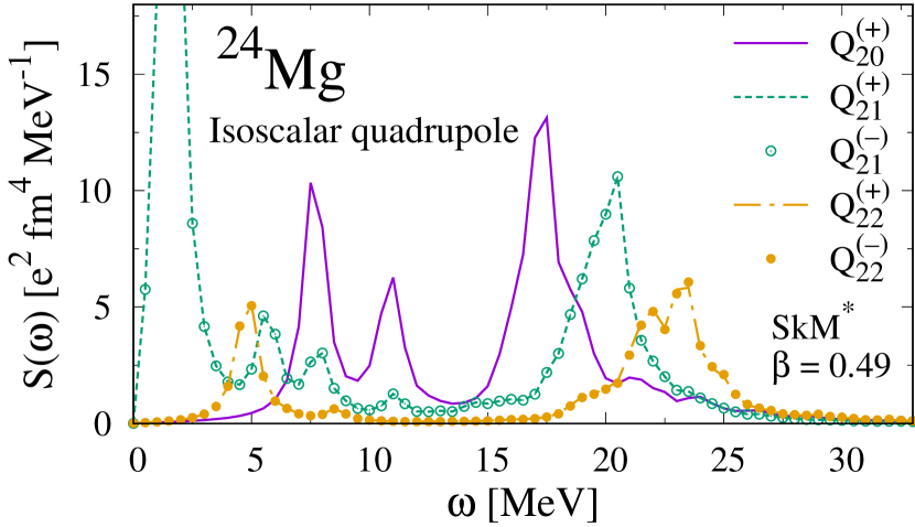
Figure 1: (Color online) Isoscalar quadrupole strengths of different $K$ as a function of $\omega$ for ²⁴Mg calculated with SkM^∗.

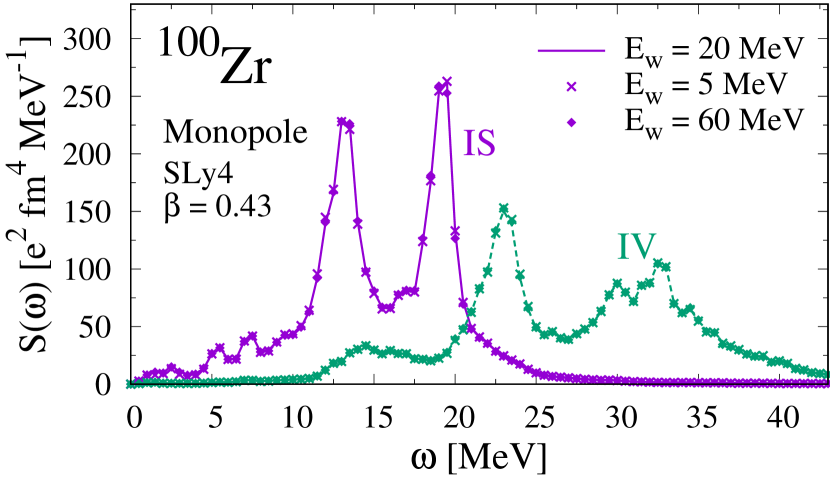
Figure 2: (Color online) Isoscalar (IS) and isovector (IV) monopole strengths as a function of $\omega$ for ¹⁰⁰Zr with SLy4 and with different pairing window energies $E_{w}=20$ MeV (solid line), 5 MeV (cross), and 60 MeV (diamond).

Figure 2 shows isoscalar and isovector monopole strengths in a prolately deformed superfluid nucleus ¹⁰⁰Zr computed with $17^{3}$ mesh ($R_{\textrm{max}}=14.0$ fm) and 1120 HF-basis states with SLy4 EDF. The obtained ground state has finite pairing gap for protons (normal phase in neutrons) and $\beta=0.43$. Compared with previous axial matrix-form QRPA Yoshida (2010) and FAM-QRPA Stoitsov et al. (2011), nice agreement on the peak energies is obtained, even though we used different pairing functionals and different pairing cutoff from those in Refs. Yoshida (2010); Stoitsov et al. (2011). In Fig. 2, we also show the dependence on the pairing window energy. The pairing strength of each pairing window was adjusted with the method mentioned above. No significant dependence of pairing window energy is observed in the strengths. Furthermore, the $0^{+}$ spurious modes corresponding to the pair rotation are not seen in the monopole strength function. This indicates good decoupling between the pair and monopole modes of excitation.

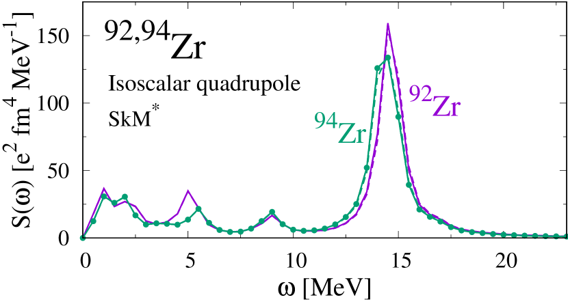
Figure 3: (Color online) Isoscalar quadrupole strengths for spherical nuclei ⁹²Zr (purple) and ⁹⁴Zr (green). All the strengths with $K=(0,1,2)$ (solid, dashed, and dot-dashed lines) and $r_{x}=\pm 1$ are identical.

We show the isoscalar quadrupole strengths of ⁹²Zr and ⁹⁴Zr in Fig. 3, which are next to an LLFP ⁹³Zr. The model space was same as in ¹⁰⁰Zr, but SkM^∗ EDF was used. The ground states of ⁹²Zr and ⁹⁴Zr are spherical and superfluid in both neutrons and protons. Since these nuclei are spherical in their ground state, the strengths of different $K$ agree with each other. The giant resonance peaks appear at around 15 MeV, while we also observe that the lowest peak is located at about $\omega\approx 1$ MeV. These low-energy modes are expected to play an important role in the shape fluctuation, which will be our future target.

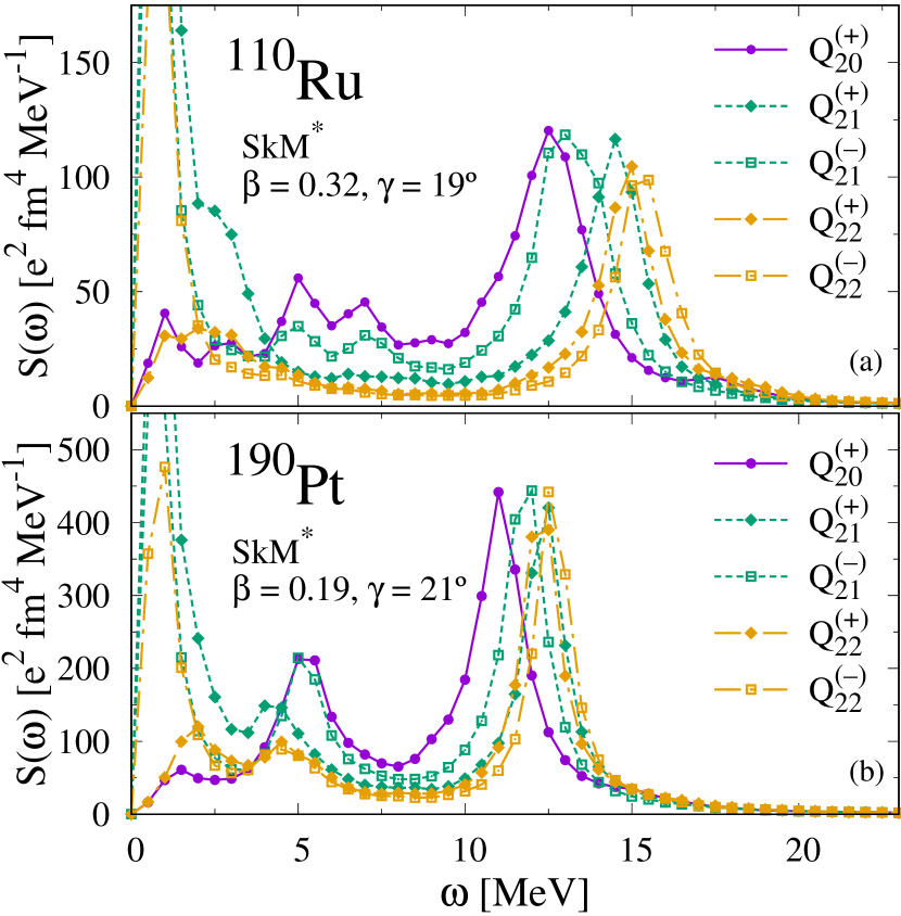
Figure 4: (Color online) Isoscalar quadrupole strengths for triaxial nuclei ¹¹⁰Ru (a) and ¹⁹⁰Pt (b).

Finally, we show the isoscalar quadrupole modes in triaxially deformed superfluid nuclei. A typical mass region of appearance of triaxial ground state is the $A\approx 100$ region and Pt isotopes Scamps and Lacroix (2014); Ebata et al. (2014). We take here ¹¹⁰Ru and ¹⁹⁰Pt, calculated with the SkM^∗ EDF. We set the longest, middle, and shortest axes to be $z$, $x$, and $y$ axes, respectively. Note that the magnetic quantum number $K$ is not good quantum number for triaxial nuclei. For our convenience, however, we use the $K$ values to specify the type of quadrupole operators $Q_{2K}^{(\pm)}$.

Figures 4(a) and 4(b) show the isoscalar quadrupole strengths of ¹¹⁰Ru and of ¹⁹⁰Pt, respectively. In both nuclei, neutrons are in the superfluid phase, while protons are not. The obtained quadrupole deformation parameters are $\beta=0.32$, $\gamma=19^{\circ}$ for ¹¹⁰Ru with the same model space as in Fig. 3. For ¹⁹⁰Pt with an enlarged model space as $19^{3}$ mesh ($R_{\textrm{max}}=15.6$ fm) and 1360 HF-basis states, we obtain the ground state with $\beta=0.19$, $\gamma=21^{\circ}$. In both nuclei, our calculation clearly produces additional signature splitting of the strength in which the peaks with different $x$ signature no longer coincide, due to the triaxial deformation. We obtain three spurious modes near zero energy due to the existence of rotations around $x$, $y$, and $z$ axes. The EWSR values are well satisfied, 98–99% for $K=0$ and $(K,r_{x})=(2,+)$ modes. We have also confirmed that the isoscalar quadrupole response has no significant dependence on the pairing window in a range from 10 to 50 MeV.

Table 1: EWSR values summed up to $\omega=50$ MeV for the isoscalar quadrupole $K=0$ strength in units of MeV $e^{2}$ fm⁴ in ¹¹⁰Ru with different numbers of HF-basis states $N_{\textrm{HF}}$ and of two-quasiparticle states $N_{\textrm{2qp}}$. The last two rows show the maximum quasiparticle energies $E_{\textrm{QP}}^{\textrm{max}}$ (in MeV) of neutrons (n) and protons (p).

$N_{\textrm{HF}}$	$N_{\textrm{2qp}}$	EWSR	$E_{\textrm{QP,n}}^{\textrm{max}}$	$E_{\textrm{QP,p}}^{\textrm{max}}$
240	7400	6913	41.3	34.2
440	24650	7121	41.3	39.8
728	67130	7159	41.3	49.5
910	104713	7162	45.9	55.3
1120	158368	7164	50.6	60.2

For the isoscalar quadrupole $Q_{20}$ of ¹¹⁰Ru, we examine in detail the convergence property of EWSR with respect to the number of HF-basis states. Table 1 shows the calculated EWSR values with FAM. For neutrons in $N_{\textrm{HF}}\leq 728$ and protons in $N_{\textrm{HF}}=240$, the main component of the highest quasiparticle state is the deepest hole state in the HF basis. We reach an approximate convergence of EWSR at $N_{\textrm{HF}}\geq 728$ which corresponds to the number of two-quasiparticle states $N_{\textrm{2qp}}\geq 67,130$. In the present 3D calculation, even though the size of the space is reduced by incorporating the parity and the $z$-signature symmetry, the number of two-quasiparticle states easily exceed 100,000. It requires enormous computational power and memory capacity to explicitly construct such large QRPA matrices. The FAM significantly reduces the computational burden and provides a feasible numerical approach to the QRPA.

Conclusions. Toward fully microscopic and non-empirical construction of the five-dimensional quadrupole collective Hamiltonian, we have developed a 3D FAM-QRPA code applicable to triaxially deformed nuclei with superfluidity. We demonstrated that the results showed good agreement with the previous axial QRPA results on multipole modes of excitation in axially symmetric nuclei, ²⁴Mg and ¹⁰⁰Zr. In axially deformed nuclei, the quadrupole strength functions with the same $K$ but different $x$ signature $r_{x}=\pm 1$ coincide to each other. The rotational zero-energy modes around $x$ and $y$ axes exist, but that around the $z$ (symmetry) axis does not.

We applied our 3D FAM-QRPA to isoscalar quadrupole modes in triaxially deformed superfluid nuclei, ¹¹⁰Ru and ¹⁹⁰Pt. Five different peaks in the strength functions appear depending on $K$ and the signature $r_{x}$. Three rotational modes also emerge at zero energy, associated with rotations about all the three axes $(x,y,z)$ because of the triaxial deformation.

The present FAM computation depends mainly on the numbers of the mesh points and of HF-basis states. The computation of the isoscalar quadrupole strength for 100 $\omega$ points in Fig. 4(b) is about 200 CPU hours in total and 3.5 GB memory. This indicates the efficiency of our computational method and feasibility in currently available computational resources.

We intend to develop a parallelized local QRPA computer code based on the present FAM-QRPA framework, to derive the collective inertial functions at every $(\beta,\gamma)$ point. To obtain low-lying discrete normal modes in the local QRPA, the contour integration technique of Ref. Hinohara et al. (2013) may be useful. The extension of the present FAM-QRPA to the local QRPA is in progress.

Acknowledgments. The authors acknowledge Nobuo Hinohara for fruitful discussions. This work was funded by ImPACT Program of Council for Science, Technology and Innovation (Cabinet Office, Government of Japan). Numerical calculations were performed in part using the COMA (PACS-IX) at the Center for Computational Sciences, University of Tsukuba.

References

- Heyde and Wood (2011) K. Heyde and J. L. Wood, Rev. Mod. Phys. 83, 1467 (2011).
- (2) http://www.jst.go.jp/impact/en/program/08.html.
- Bender et al. (2003) M. Bender, P.-H. Heenen, and P.-G. Reinhard, Rev. Mod. Phys. 75, 121 (2003).
- Bender and Heenen (2008) M. Bender and P.-H. Heenen, Phys. Rev. C 78, 024309 (2008).
- Rodríguez and Egido (2010) T. R. Rodríguez and J. L. Egido, Phys. Rev. C 81, 064323 (2010).
- Yao et al. (2010) J. M. Yao, J. Meng, P. Ring, and D. Vretenar, Phys. Rev. C 81, 044311 (2010).
- Anguiano et al. (2001) M. Anguiano, J. L. Egido, and L. M. Robledo, Nucl. Phys. A 696, 467 (2001).
- Dobaczewski et al. (2007) J. Dobaczewski, M. V. Stoitsov, W. Nazarewicz, and P.-G. Reinhard, Phys. Rev. C 76, 054315 (2007).
- Próchniak et al. (2004) L. Próchniak, P. Quentin, D. Samsoen, and J. Libert, Nucl. Phys. A 730, 59 (2004).
- Nikšić et al. (2009) T. Nikšić, Z. P. Li, D. Vretenar, L. Próchniak, J. Meng, and P. Ring, Phys. Rev. C 79, 034303 (2009).
- Delaroche et al. (2010) J. P. Delaroche, M. Girod, J. Libert, H. Goutte, S. Hilaire, S. Péru, N. Pillet, and G. F. Bertsch, Phys. Rev. C 81, 014303 (2010).
- Matsuo et al. (2000) M. Matsuo, T. Nakatsukasa, and K. Matsuyanagi, Prog. Theor. Phys. 103, 959 (2000).
- Nakatsukasa (2012) T. Nakatsukasa, Prog. Theor. Exp. Phys. 2012, 01A207 (2012).
- Nakatsukasa et al. (2016) T. Nakatsukasa, K. Matsuyanagi, M. Matsuo, and K. Yabana, Rev. Mod. Phys. 88, 045004 (2016).
- Hinohara et al. (2010) N. Hinohara, K. Sato, T. Nakatsukasa, M. Matsuo, and K. Matsuyanagi, Phys. Rev. C 82, 064313 (2010).
- Hinohara et al. (2011) N. Hinohara, K. Sato, K. Yoshida, T. Nakatsukasa, M. Matsuo, and K. Matsuyanagi, Phys. Rev. C 84, 061302 (2011).
- Hinohara et al. (2012) N. Hinohara, Z. P. Li, T. Nakatsukasa, T. Nikšić, and D. Vretenar, Phys. Rev. C 85, 024323 (2012).
- Yoshida and Hinohara (2011) K. Yoshida and N. Hinohara, Phys. Rev. C 83, 061302 (2011).
- Yoshida and Giai (2008) K. Yoshida and N. V. Giai, Phys. Rev. C 78, 064316 (2008).
- Péru and Goutte (2008) S. Péru and H. Goutte, Phys. Rev. C 77, 044313 (2008).
- Peña Arteaga et al. (2009) D. Peña Arteaga, E. Khan, and P. Ring, Phys. Rev. C 79, 034311 (2009).
- Losa et al. (2010) C. Losa, A. Pastore, T. Døssing, E. Vigezzi, and R. A. Broglia, Phys. Rev. C 81, 064307 (2010).
- Terasaki and Engel (2010) J. Terasaki and J. Engel, Phys. Rev. C 82, 034326 (2010).
- Imagawa and Hashimoto (2003) H. Imagawa and Y. Hashimoto, Phys. Rev. C 67, 037302 (2003).
- Inakura et al. (2009) T. Inakura, T. Nakatsukasa, and K. Yabana, Phys. Rev. C 80, 044301 (2009).
- Inakura et al. (2011) T. Inakura, T. Nakatsukasa, and K. Yabana, Phys. Rev. C 84, 021302 (2011).
- Inakura et al. (2013) T. Inakura, T. Nakatsukasa, and K. Yabana, Phys. Rev. C 88, 051305 (2013).
- Stetcu et al. (2011) I. Stetcu, A. Bulgac, P. Magierski, and K. J. Roche, Phys. Rev. C 84, 051309 (2011).
- Ebata et al. (2010) S. Ebata, T. Nakatsukasa, T. Inakura, K. Yoshida, Y. Hashimoto, and K. Yabana, Phys. Rev. C 82, 034306 (2010).
- Scamps and Lacroix (2013) G. Scamps and D. Lacroix, Phys. Rev. C 88, 044310 (2013).
- Scamps and Lacroix (2014) G. Scamps and D. Lacroix, Phys. Rev. C 89, 034314 (2014).
- Ebata et al. (2014) S. Ebata, T. Nakatsukasa, and T. Inakura, Phys. Rev. C 90, 024303 (2014).
- Nakatsukasa et al. (2007) T. Nakatsukasa, T. Inakura, and K. Yabana, Phys. Rev. C 76, 024318 (2007).
- Avogadro and Nakatsukasa (2011) P. Avogadro and T. Nakatsukasa, Phys. Rev. C 84, 014314 (2011).
- Stoitsov et al. (2011) M. Stoitsov, M. Kortelainen, T. Nakatsukasa, C. Losa, and W. Nazarewicz, Phys. Rev. C 84, 041305 (2011).
- Liang et al. (2013) H. Liang, T. Nakatsukasa, Z. Niu, and J. Meng, Phys. Rev. C 87, 054310 (2013).
- Nikšić et al. (2013) T. Nikšić, N. Kralj, T. Tutiš, D. Vretenar, and P. Ring, Phys. Rev. C 88, 044327 (2013).
- Kortelainen et al. (2015) M. Kortelainen, N. Hinohara, and W. Nazarewicz, Phys. Rev. C 92, 051302 (2015).
- Baran et al. (2008) A. Baran, A. Bulgac, M. M. Forbes, G. Hagen, W. Nazarewicz, N. Schunck, and M. V. Stoitsov, Phys. Rev. C 78, 014318 (2008).
- Bonche et al. (1987) P. Bonche, H. Flocard, and P.-H. Heenen, Nucl. Phys. A 467, 115 (1987).
- Gall et al. (1994) B. Gall, P. Bonche, J. Dobaczewski, H. Flocard, and P.-H. Heenen, Z. Phys. A 348, 183 (1994).
- Terasaki et al. (1995) J. Terasaki, P.-H. Heenen, P. Bonche, J. Dobaczewski, and H. Flocard, Nucl. Phys. A 593, 1 (1995).
- Bonche et al. (2005) P. Bonche, H. Flocard, and P.-H. Heenen, Comput. Phys. Commun. 171, 49 (2005).
- Ryssens et al. (2015) W. Ryssens, V. Hellemans, M. Bender, and P.-H. Heenen, Comput. Phys. Commun. 187, 175 (2015).
- Bonche et al. (1985) P. Bonche, H. Flocard, P.-H. Heenen, S. Krieger, and M. Weiss, Nucl. Phys. A 443, 39 (1985).
- Hellemans et al. (2012) V. Hellemans, P.-H. Heenen, and M. Bender, Phys. Rev. C 85, 014326 (2012).
- Bartel et al. (1982) J. Bartel, P. Quentin, M. Brack, C. Guet, and H.-B. Håkansson, Nucl. Phys. A 386, 79 (1982).
- Chabanat et al. (1998) E. Chabanat, P. Bonche, P. Haensel, J. Meyer, and R. Schaeffer, Nucl. Phys. A 635, 231 (1998).
- Yoshida (2010) K. Yoshida, Phys. Rev. C 82, 034324 (2010).
- Hinohara et al. (2013) N. Hinohara, M. Kortelainen, and W. Nazarewicz, Phys. Rev. C 87, 064309 (2013).