The Reachability of Computer Programs

Abstract

Would it be possible to explain the emergence of new computational ideas using the computation itself? Would it be feasible to describe the discovery process of new algorithmic solutions using only mathematics? This study is the first effort to analyze the nature of such inquiry from the viewpoint of effort to find a new algorithmic solution to a given problem. We define program reachability as a probability function whose argument is a form of the energetic cost (algorithmic entropy) of the problem.

1 Introduction

“The Golden Egg was not as exciting as the goose that laid it.” This phrase, uttered by Ray J. Solomonoff [28], is the motto of this paper. We want to investigate the possibility of explaining the discovery of computational ideas using only physics, and computation itself. The starting point of this investigation lies in the question:

“How difficult it is for a programmer discover a new algorithmic solution for a problem?”

It is necessary to explain in what sense the words “algorithmic solution” and “problem” we are using here. To clarify the meaning of these terms, we will take the Fibonacci’s series as an example. The first ten elements of it are completely well-described by the string:

$$0,1,1,2,3,5,8,13,21,34$$

The program that prints the string above is an algorithmic solution for the problem. The question “how to generate the string that represents the first ten terms of the Fibonacci series?” represents this latter problem. Simplifying the problem; we considered the string itself as the actual problem. Thus, find an algorithmic solution is to discover a program for (to print) a problem (string).

The aim of this paper is to analyze the phenomenon of new programs emergence (discovery by a programmer) in the physical world. We follow the train of thought contained in [12, 26], which argues that computers are physical objects, computations are physical processes, and they exist in the real-world. The fact that such appearance occurs in our material universe and not in an entirely symbolic space, disassociated from any physical meaning, is our primary postulate. We will show that the logical consequence of this physicalist argument is that the probability of a programmer to develop a new program obeys an underlying entropy principle, informational at first, but also thermodynamics; thus leading us to the concept of algorithmic reachability.

As initial motivation, we concentrate on minimum length program probability. The objective is to associate the (incomputable) minimum length program concept with our reachability investigation. We will show that the emergence of minimum programs (determined by the Kolmogorov complexity) is a function of the energetic intrinsic cost to achieve it.

This paper is structured as follows. Section 2 describes the notations and theoretical preliminaries; Section 3 presents the motivation of this work; Section 4 presents the programs reachability, and Section 5 describes its formulation. The Section 6 discusses the results presented in the previous section and the last section presents the conclusion.

2 Background

In this section, we give several definitions and notations required for the adequate discussion of the present article. We assume that the reader is familiar with basics concepts of physics, calculus, and probability.

2.1 General definitions

Definition 1 (Lambert $W$ function).

Let $\mathbb{R}$ be the sets of all real numbers. For $x\in\mathbb{R}$, the Lambert $W$ function [25] is defined as the inverse of the function $f(x)=xe^{x}$ and solves :

$$W(x)e^{W(x)}=x.$$ (1)

$W(x)$ has the following behavior:

• For $x\geqslant 0$, $W(x)$ is a real positive function.

• For $-1/e<x<0$, $W$ is a multivalued application with two negative real-valued branches: $W_{0}(x)$ and $W_{-1}(x)$ [11].

• For $x=-1/e$, $W(x)=-1$.

• For $x=0$, $W(x)=0$.

• For $x<-1/e$, $W(x)$ is not defined in $\mathbb{R}$.

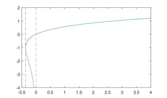
Figure 1: Graph of the Lambert W Function

Definition 2 (Binary string and its length).

Let the binary alphabet $B=\{0,1\}$ and $\mathbb{N}$ be the sets of all natural numbers. A string $\rho$ is any finite sequence of juxtaposed elements of the alphabet $B$ and its length $l(\rho)=n$ is the number $n\in\mathbb{N}$ of the elements composing $\rho$.

Definition 3 (Reflexive and Transitive Closure over the alphabet).

Let $B^{k}=\{s:l(s)=k\}$ be the set of all strings with length $k$. The reflexive and transitive closure over the alphabet $B$ is defined as $B^{\ast}=\bigcup_{k=0}^{\infty}B^{k}$. In a similar way, $B^{+}=\bigcup_{k=1}^{\infty}B^{k}$ defined as the set of all nonempty strings over $B$

Definition 4 (Prefix String and Prefix free set).

Let the strings $r\in B^{\ast}$. In this context, a string $v$ is a prefix of r ($v\subseteq r$) if there exists $u\in B^{\ast}$ such that $r=vu$. A set $F\subseteq B^{+}$ is called a prefix-free set when, $\forall(v,r\in F)$, $v\subseteq r$ is only true for $v=r$, .

2.2 Kolmogorov Complexity

Definition 5 (Solution for $\rho$).

Given a universal Turing machine $\mathcal{U}$ and an input (program) in the form of a binary string $\varsigma$, if $\varsigma$ generates the string $\rho$ as output, so that:

$$\mathcal{U}(\varsigma)=\rho$$

then, we say that $\varsigma$ is a solution for the problem $\rho$.

Definition 6 (Chaitin machine and minimal program).

If a universal Turing machine $\mathcal{U}$ is defined for $\varsigma$ but not defined for any prefix $v$ of $\varsigma$, then this machine is called a Chaitin machine [29] and denoted by $\mathfrak{U}$. Any $\varsigma$ accepted by $\mathfrak{U}$ is referred to as a minimal program.

Definition 7 ($\rho$-solution set).

The set ${\Lambda}^{\rho}=\{\varsigma_{1},\varsigma_{2},\dots,\varsigma_{n}\}$ of all minimal programs that are solutions of the problem $\rho$ is called a $\rho$-solution set. The set ${\Lambda}^{\rho}$ is assumed to be finite.

Definition 8 (Kolmogorov complexity).

[13, p. 110] Given a problem $\rho$ with ${\Lambda}^{\rho}$, the Kolmogorov complexity of $\rho$ is defined as:

$$K(\rho)=min\{l(\varsigma_{i}):\mathfrak{U}(\varsigma_{i})=\rho\}$$ (2)

Thus, the Kolmogorov complexity of $\rho$ is the $\rho$-solution set element with the lowest length. $\varsigma_{kol}$ now denotes this program.

2.3 Boltzmann and Shannon entropy

Definition 9 (Shannon’s Entropy).

[27, p. 18] For a finite sample space $\Omega$, let $X$ be a random variable taking values in $\Omega$ with probability distribution $p(x)$ for all $x\in X$. The Shannon entropy is defined as:

$$H=-\sum_{x}p(x)\log_{2}p(x)$$ (3)

Definition 10 (Boltzmann’s Entropy).

For the special case of a discrete state space with L the counting measure defined as $L(\Gamma_{x})=d(\Gamma_{x})$, that is, the number of elements in the set $\Gamma_{x}$,

$$SB(x)=(k\ln 2)\log d(\Gamma_{x})$$ (4)

is the familiar form of the Boltzmann entropy [24].

The Gibbs entropy is defined as:

$$SG=k\ln\Gamma$$ (5)

Where $\Gamma$, which is the number of microstates corresponding to a given macrostate of a thermodynamic system [17, p. 457], and $k=1.38065\times 10^{-23}J/K$ is the Boltzmann constant.

2.3.1 Relationship between Gibb’s and Shannon’s Entropy

.

The relation between the Expression 3 and 5 is expressed as follow [18, 1]:

$$SB=Hk\ln 2$$ (6)

Following [24, section 8.6], the previous approaches (Gibbs, or Boltzmann’s entropy and Shannon’s entropy concepts) “treated entropy as a probabilistic notion; in particular, each microstate of a system has entropy equal to $0$. However, it is desirable to find a concept of entropy that assigns a nonzero entropy to each microstate of the system, as a measure of its individual disorder.” The last sentence means that Kolmogorov Complexity may be used to define the concept of algorithmic entropy.

Considering that any measure of an individual microstate of a particular system has nonzero entropy and supposing that this system in equilibrium is described by the encoding $x$ of the approximated macroscopic parameters, one can estimate the entropy of the macrostate encapsulating the microstate. The algorithmic entropy of the macrostate of a system is given by $K(x)+H_{x}$, where $K(x)$ is the prefix complexity of $x$, and $H_{x}=\frac{SB(x)}{(k\ln 2)}$. Here SB(x) is the Boltzmann entropy of the system constrained by macroscopic parameters x, and k is Boltzmann’s constant. The physical version of algorithmic entropy is defined as $SA(x)=(k\ln 2)(K(x)+H_{x})$.

Gibbs entropy is essentially the average algorithmic entropy. Let $H_{\mu}(x)=K(x)+O(1)$. Thus, the algorithmic entropy $H_{\mu}$ is a generalization of the prefix complexity $K$ [24]. The connection between Gibbs entropy and $H_{\mu}$ is given by the equation below [24]:

$$SA(w)=(k\ln 2)H_{\mu}(w),SA^{n}(w)=(k\ln 2)H_{\mu}^{n}(w)$$ (7)

2.4 Probability and physical work

Definition 11 (Conditional Probability).

[19, p. 22] Let $\Omega=(e_{1},e_{2},\dots,e_{m})$ be a countable set of disjoint an exhaustive events, where each $e_{i}$ is associated with a probability $P(e_{i})$ such that $\sum_{i}P(e_{i})=1$ and $P(e_{i})\neq 0$. Given $y$ as any event with $P(y)>0$, for all $i$:

$$P(e_{i}|y)=\frac{P(y|e_{i})P(e_{i})}{P(y)}$$ (8)

The relationship physical work and Shannon entropy variation. In a thermodynamic process [30, p. 375] with a transition taking a system from an initial state $1$ to some final state $2$, the work $\Delta W$ extracted in the course of the transition can be expressed regarding thermodynamic entropy as follow [33]:

$$\Delta W=T\Delta E$$ (9)

Where $T$ is the temperature in Kelvin scale on Equation 9 which is valid for a process with a transition sufficiently slowly to be thermodynamically reversible and with the internal energy of the system considered as constant. The variation $\Delta E$ is the difference between the entropy of the final and initial state[6]:

$$\Delta E=S_{2}-S_{1}$$ (10)

By Expression 6, we have:

$$\Delta W=kT\ln 2\Delta H$$ (11)

3 Motivation

In computer science, new programs are often designed. Some of them solve problems for which there was already a solution found. Some algorithms exist for centuries, some others are very recent, turning them part of the solution cluster for a determined class of computable problems. Others, on the other hand, provide more efficient solutions from the asymptotic analysis point of view, that is, on the amount of time or memory needed to get an output.

Regardless of the asymptotic complexity class, each computable problem has an algorithmic solution whose length in bits, prefix-free, is minimum, and that value is the Kolmogorov complexity equation 2 itself. The concept of Kolmogorov complexity relates to the principle of Occam’s Razor [24, p. 260]. We can interpret such principle as a method for selecting solutions, where the simplest case, among other explanations for the phenomenon under study, has to be chosen. Such principle presupposes the existence of a simplicity criterion in nature and Kolmogorov complexity appears as an objective measure to treat such simplicity. Unfortunately, for all string $\rho$, it is not possible to calculate $K(\rho)$, due to its incomputability.

However, nothing prevents us from investigating the occurrence probability of $\varsigma_{kol}$, i.e. the probability that a programmer develops exactly the minimum program, the element of $\rho$-solution set ${\Lambda}^{\rho}$ with the smallest length in bits, whose length value is precisely the Kolmogorov Complexity $K(\rho)$.

3.1 Postulated Effects

In the introduction, we said that our main postulate is the fact that the discovery of new programs happens in the real-world. Although it is a postulate, we need to analyze most strictly the influence of this statement in our investigation of the minimum length program occurrence probability.

The expression of such probability involves the $\rho$-solution set ${\Lambda}^{\rho}$ and the derivation of Bayes’ conditional rule (Expression 8):

$$P(\varsigma_{kol})=\frac{P(\varsigma_{kol}|\rho)\cdot P(\rho)}{P(\rho|\varsigma_{kol})}$$ (12)

The postulated effects of the Expression 12 are given below:

Postulated Effect 1

: the term $P(\rho|\varsigma_{kol})$ is the occurrence probability of $\rho$ given the occurrence of $\varsigma_{kol}$. However it is necessary to put this term in a complete context: $P(\rho|\varsigma_{kol})$ is the probability of a Chaitin machine $\mathfrak{U}$, whose input is $\varsigma_{kol}$, generates the string $\rho$ as output. The program $\varsigma_{kol}$ is the minimum length program that generates $\rho$. It generates $\rho$ and no other. It does not run forever, because $\varsigma_{kol}$ is an element of ${\Lambda}^{\rho}$ and not an arbitrary program. Thus, for $\mathfrak{U}(\varsigma_{kol})=\rho$, $P(\rho|\varsigma_{kol})=1$. In this manner, Expression 12 takes the form :

$$P(\varsigma_{kol})=P(\varsigma_{kol}|\rho)\cdot P(\rho)$$ (13)

Postulated Effect 2

: the term $P(\varsigma_{kol}|\rho)$ is the occurrence probability of $\varsigma_{kol}$ given the occurrence of $\rho$. At the same time, $\mathfrak{U}(\varsigma_{i})=\rho$ (for every $\varsigma_{i}\in{\Lambda}^{\rho}$), which means that $p(\varsigma_{kol}|\rho)$ represents the probability that the Chaitin machine $\mathfrak{U}$ have generated the string $\rho$ from the occurrence of the input $\varsigma_{kol}$.

The construction (or reification) of a program comes from after a problem attestation by a witness. The fact that problem $\rho$ can be described as a binary string is a consequence of it being noticed and somehow recorded by a group of witnesses that agree among themselves about its existence, and also how to represent it. Therefore, we can only talk about the situations where there is absolute certainty of the occurrence of $\rho$, that is, the situation where this occurrence is a prerequisite, where we have:

$$P(\varsigma_{kol}|\rho)=P(\varsigma_{kol})$$ (14)

$$P(\varsigma_{kol}|\neg\rho)=0$$ (15)

$$P(\rho)=1$$ (16)

Thus, we have that the occurrence probability of $\varsigma_{kol}$ is always an a posteriori probability, conditioned by the problem of generating $\rho$ as an output of $\mathfrak{U}$ by $\varsigma_{kol}$ input.

4 The reachability of a program

However, what does to calculate the probability of a programmer to develop the program $\varsigma_{kol}$ mean, in a semantic sense? Programs are not balls in a ballot box. They are not cards of a deck, dice faces or $\alpha$-particles shocking against a photographic plate. The Kolmogorov’s complexity study about $\rho$ randomness nature is independent of the way $\varsigma_{kol}$ can be obtained [23]. A raffle, a toss of a coin, or occurrence frequency calculus does not give the presence or absence of $\varsigma_{kol}$, and it neither appears spontaneously in the input tape of the Chaitin machine $\mathfrak{U}$.

The objective of a program is to solve a problem. There is a pragmatical necessity that the developed program generates a string $\rho$. Thus, the existence of $\varsigma_{kol}$ already implies (by its definition) the occurrence of a nontrivial phenomenon of compression that led to its description from $\rho$. To $\varsigma_{kol}$ be the input of $\mathfrak{U}$ there exist a sequence of events involved in the conception of the program and its constructive generation. This situation shows to us that the probability of a programmer developing a new algorithmic solution to a given problem correlates with the necessity notion, in an Aristotelian sense.

Necessary is that which can not be otherwise [15, p. 468]. The necessity is what makes it impossible for something to be other than it is [16, p. 120]. Necessity is the reverse of the impossibility. To illustrate the concept of impossibility, take the following illustration: a man can return to his childhood home and remodel it so that it looks, as much as possible, like what he has in mind, but he still cannot go back in the past. Hence, going backward to relive his past consists in an impossibility.

The path followed by the programmer to find a new algorithmic solution lies under necessity constraints. In this sense, the Occam’s razor is necessity principle, as well Shannon’s entropy $H$ is a measure of the average impossibility [2, p. 141]. Thus, there is a necessary way for a programmer to develop a new program and, at this moment, we need a clear connection between occurrence probability and necessity concept, to get the fact and showing how much it is necessary, what needs to happen and cannot be otherwise. This connection element is the $P(\varsigma_{kol})$ probability 14. We will not associate its meaning with a raffle phenomenon, but we will see it as a measure of the program reachability.

5 The program reachability calculus

In this way, we define the program reachability of $\varsigma_{i}\in\Lambda^{\rho}$ as the quantifiable relative necessity of an input $\varsigma_{i}$ for a Chaitin machine $\mathfrak{U}$ when $\varsigma_{i}$ generates $\rho$ as its output. Such relative necessity is represented by $P(\varsigma_{kol})$. However, a probability that cannot be expressed has no purpose. Thus, it is necessary to describe a way to obtain the program reachability expression regarding necessity or impossibility. The Shannon entropy, defined in 9 will provide us this way. For this, let us take the random variable $X$ constituted by the enumeration elements of ${\Lambda}^{\rho}$. The image space of $X$ is expressed by:

$$I_{X}=\{1,2,\dots,i,\dots,m\}$$ (17)

For such random variable, with respective probabilities $p(1),p(2),\dots,p(m)$, we have the Shannon entropy associated, given by the expression 3:

$$H=-[p(1)\log_{2}p(1)+\dots+p(i)\log_{2}p(i)+\dots+p(m)\log_{2}p(m)]$$ (18)

Now, let us isolate the sum component concerning to $x=i$:

$$H+[p(1)\log_{2}p(1)+\dots+p(m)\log_{2}p(m)]=-p(i)\log_{2}p(i)$$ (19)

At this point, it is important to note that the component

$$[p(1)\log_{2}p(1)+\dots+p(i-1)\log_{2}p(i-1)+p(i+1)\log_{2}p(i+1)+\dots+p(m)\log_{2}p(m)]$$ (20)

The right side of equation 19 refers to the entropy of a random variable $X^{\prime}$, which represents the enumeration of $A^{\rho}$, without its $i$th element. The $X^{\prime}$ space image description may be expressed as:

$$I_{X^{\prime}}=I_{X}-\{i\}$$ (21)

Such variable also has its own Shannon entropy, and the expression of this entropy is the component $[p(1)\log_{2}p(1)+\dots+p(m)\log_{2}p(m)]$, which will call $H^{\prime}$. Thus, replacing the expression 19, we have:

$$p(i)\log_{2}p(i)=-(H-H^{\prime})$$ (22)

Another way to envision equation 22 is to consider it as describing the energy fluctuations by means of the difference on the entropy of the function that describes the program $\varsigma_{i}$, such that $p(i)\log_{2}p(i)=-\Delta(H_{\varsigma_{i}})$.

Equation 22 is non-linear. To determine $p(i)$ is necessary to deal with this non-linearity. Lambert $W$ function, described in Definition 1, is an important mathematical tool which allows the analytic solutions for a broad range of mathematical problems [3], including the solution of equation $x\log_{a}x=b$ (for $x,a,b\in\mathbb{R}$), which is [10]:

$$x\log_{a}x=b\Longleftrightarrow x=e^{W(a\ln b)}$$ (23)

Moreover, this is exactly the form of Equation 22. To simplify the analysis, we will denominate the expression $(H-H^{\prime})$, the entropy variation, as $\mathrsfs{H}(\varsigma_{i})$. Notwithstanding, $p(i)$ represents the occurrence probability of the event $\varsigma_{i}$. Thus, with proper algebraic manipulation, for all $\varsigma_{i}\in\Lambda^{\rho}$ (including the program $\varsigma_{kol}$) we have:

$$P(\varsigma_{i})=\exp^{W(-\mathrsfs{H}(\varsigma_{i})\ln 2)}$$ (24)

As the entropy is positive, the domain of the function will be negative, which will yield a negative number for the $W$ function. Hence taking the $W_{-1}$ branch we’ll rewrite it as:

$$P(\varsigma_{i})=\exp^{-\|W_{-1}(-\mathrsfs{H}(\varsigma_{i})\ln 2)\|}$$ (25)

Nevertheless we have an equation for $P(\varsigma_{i})$ that maps a semi-measure for the probability distribution over the finite event set, and it yields values ranging from $0<P\leq 1$. Moreover, we can normalize it to become an actual measure for the probability stating: $P(\varsigma_{i})=\frac{\exp^{-\|W_{-1}(-\mathrsfs{H}(\varsigma_{i})\ln 2)\|}}{\sum_{i}P(\varsigma_{i})}$. In this case we actually have a probability distribution measure for the events, and $\sum_{i}P(\varsigma_{i})\leq 1$.

6 Results discussion

6.1 Bounds on reachability function domain

We need to analyze the behavior of $P(\varsigma_{i})$, impose no restrictions other than those typical of the analyzed function. Because the characteristics of Lambert $W$ function described in 1, the following domain restrictions for function $P(\varsigma_{i})$ are needed:

$$-\dfrac{1}{e}\leq-\mathrsfs{H}(\varsigma_{i})\ln 2\leq 0$$ (26)

which implies:

$$0\leq\mathrsfs{H}(\varsigma_{i})\leq\dfrac{1}{e\ln 2}$$ (27)

Since $\frac{1}{e\ln 2}\approx 0.5307$, we may rewrite Inequality 27 as

$$0\leq\mathrsfs{H}(\varsigma_{i})\lessapprox 0.5307$$

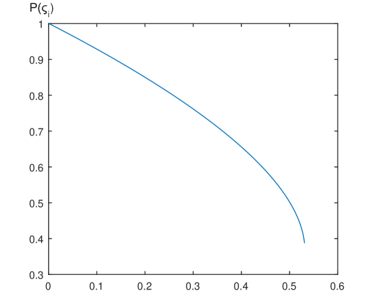
Figure 2: Graph of the function $P(\varsigma_{i})$. In $x$-axis, we have the values of $\mathrsfs{H}(\varsigma_{i})$

Consider equations (22) and (25) regarding a learning process for the algorithm reachability. We can apply equation (25) to reach a better program in a similar way the gradient descent algorithm is applied to machine learning algorithms. There is an algorithmic entropy associated with the process of learning [24, 7, 21].

One important feature of this approach on the Principle of Least Cognitive Action [21] is that gradient descent algorithm can be derived from the principle.

In this sense, we envision the exponential of the Lambert W function as a matching loss for the learning algorithm [20], but it is not convex, besides being continuous, for the domain [5, Proposition $5$].

Since Lambert $W$ function is not convex, but continuous for the domain $x<0$; our proposal for the probability semi-measure is $P(\varsigma_{i})=\exp^{-\|W_{-1}(-\mathrsfs{H}(\varsigma_{i})\ln 2)\|}$, which is bounded by the negative exponential of the Lambert’s $W$ function. Proposition 7 from [5] deals with it:

Lemma 1.

$\exp^{-W(x)}$ is convex. (This is proposition 7 from [5])

Proof.

See proof of proposition 7 on [5] ∎

Hence we have:

Theorem 1.

Let $\ell$ be a loss function as $\ell=\exp^{-W(x)}$, then $\ell$ is a matching loss.

Proof.

From Property $(P1)$ of [20] we have this strong claim: $\ell(\hat{y},y):\mathbb{R}\times\mathbb{R}\rightarrow[0,\infty)$ is continuous and bounded. And from Theorem 5.1 of [20] if a loss function follows the property then it is a matching loss.

To prove the theorem we make:

$y=f(z)=\exp^{-W(z)}$

$z=f^{-1}(y)=W^{-1}(\frac{1}{\exp^{-y^{-1}}})=W^{-1}(\frac{1}{\ln(y)})$

$\ell(\hat{y},y)=\ell(f(\hat{z}),f(z))=\exp^{W(\hat{z})}-\exp^{W(z)}-f^{{}^{\prime}}(z)(\hat{z}-z)$

which is convex in $\hat{z}$ by Lemma 1 (Proposition $7$ of [5]). Hence, by Theorem 5.1 of [20], $\ell$ is a matching loss function. ∎

With these equations, our approach yields a theoretically sound method for the reachability calculus for a program. Nonetheless, Lambert W function is not entirely computable, for instance, $W(1)=\Omega$, Chaitin’s incomputable constant.

The simpler algorithm to reach a program builds all programs of the same size and checks them all; afterward, switches them to an immediately smaller size. On a subsequent step, the algorithm produces the smallest program only when there is no transformation left to reduce the size unless there is an informed hypotheses search-space. This process produces a meaningful result that is: the smallest program is not necessarily the most accessible one.

Consider now that one method that defines an algorithm which is guided by the least energy cost given by Equation 25, applying a gradient descent. From this method we may argue its connection with the well-known Levin-Search algorithm [4, 24] since we also provide a search method (reachability), but for a program.

6.2 The Demiurge

The connection between the concepts of probability and necessity does not eliminate the question of spontaneous generation of programs: after all, who is responsible for creating new programs, since their creation does not originate from throwing dices or tossing coins? Thus, beyond the concept of reachability, we need a constructive cause, a responsible agent, a being that we call Demiurge. Consider this being as a version of Maxwell’s demon. We can also understand the following digression from the arguments and measures exposed in [14].

The philosopher Plato (in his dialog Timaeus) [32, p. 120] described the Demiurge (which in Greek means “craftsman”) as a world-generation entity, sometimes represented as endowed with only limited abilities. The Demiurge shapes the cosmos via imposing pre-existing form on matter, according to some ideal and perfect model [8]. However, although it has such capacity, the Demiurge is not omnipotent, omnipresent and omniscient.

The use of Demiurge in this paper has no intention of inserting any supernatural element in this discussion. The use of this term allows us to establish a cause for the generation of programs without the need of discussing the nature of this cause (for instance, whether the Demiurge is a machine or not), only its functions. In principle, the Demiurge is a physical system.

Thus, our Demiurge (represented by symbol $\mathfrak{D}$) has the ability of “to bring” new algorithmic solutions for a problem $\rho$. However, the Demiurge action as the “discoverer” of a new solution for the problem $\rho$ involves an effort to carry out its function. There must be an energy consumption; which means that it needs to realize work to discover a new program $\varsigma_{i}$.

Such fact has its effects on Expression 24, which states that the reachability of a program is a function of the entropy variation (represented by $\Delta H$ in Expression 11 and, since Expression 24, represented by $\mathrsfs{H}(\varsigma_{i})$). However, we know (by Definitions 9 and 11) that is possible to describe an entropy variation in function of extracted work.

$$\mathrsfs{H}(\varsigma_{i})=\dfrac{\Delta W}{kT\ln 2}$$ (28)

Similarly to what was made with the definition of $\mathrsfs{H}(\varsigma_{i})$, we will describe the variation of the work in terms of $\varsigma_{i}$ as follows:

$$\Delta W=\mathrsfs{E}(\varsigma_{i})$$ (29)

As the Demiurge $\mathfrak{D}$ is the responsible for this work and the variation of entropy is associated to the program reachability $\varsigma_{i}$ as well, the entropy variation of Expression 24 we may substitute it by the right side of Expression 28.This results in:

$$P(\varsigma_{i}|\mathfrak{D})=e^{W(-\mathrsfs{E}(\varsigma_{i})/{kT})}$$ (30)

The new version presented above makes the connection between the program reachability and the process of discovering new programs by the Demiurge $\mathfrak{D}$. Through this; we can observe that each solution to $\rho$ is associated with a determined quantity of energy expended to generate it. For the Expression 30, the options for the energy values have their boundaries well determined (by Expression 27). Inside these limits, depending on the quantity of work available (and the amount of work realized by the Demiurge), we may have a bigger or smaller probability of reaching a new solution.

7 Conclusion

As stated in the introduction of this paper our goal was to set an abstraction for algorithmic discovery bounded by its reachability and its size. The idea behind the proposal is to view different programs simply as modified versions of the same basic program, this way any transformation between programs of the same size will not demand more energy to occur. However, to generate programs in a smaller size, it is necessary to apply work of the order $kT\ln 2$ as stated on expression 28. This result agrees with the Landauer’s principle [14].

The simpler algorithm is then to build all programs of the same size and check them all, afterward switch them to an immediately smaller size. The next step of the algorithm produces the smallest program only when there is no transformation left to reduce the size unless there is an informed hypotheses search-space. This result means that generically speaking the smallest program not necessarily is the most accessible one.

At this point the Demiurge cuts the knot by applying the work difference to the problem as an entropy result, thus producing an informed search on a non-informed hypotheses search-space. In fact using a gradient descent by Equation 25. We can envision this idea as applying a Kolmogorov complexity measure, using the Lambert $W$ function, at each transformation step of a program, seeking a path around the lower complexity programs.

7.1 Future Investigation

The presented results of this work span a series of connections to some areas that deserve further investigation. There are associations between temperature and entropy of a system in  [9, Section 2.1.11] through the thermodynamics’s concept of microstates, and there is a study of these thermodynamics’s concepts to algorithmic context [7], but it is yet to be connected to this work.

Still, in the line of states, the correlation between the current work and the minimum amount of states of a Turing machine must also be drawn. Such study is of interest not only because of the Kolmogorov complexity, one of the central arguments of this research, but also to define the theoretical lower-bound of Turing-machine states for any given program specification; this kind of information is useful, for instance, to study certain properties of specific algorithms such as the Busy Beaver [31].

Last but not the least, study ways to explore the Demiurge’s informed search to develop programs with smaller sizes for a given output; although ambitious, it conceptually intersects with the works of Levin [4, 24], and on minimum message length [9] and minimum description length [22].

References

References

- [1] Atlan H.; Fessard A. L’organisation biologique et la théorie de l’information, volume 1351. Hermann Paris, (1972).
- [2] Ben-Naim A. A Farewell to Entropy: Statistical Thermodynamics Based on Information. World Scientific, (2008).
- [3] Brito P.; Fabiao F.; Staubyn A. Euler, Lambert, and the Lambert W-function today. Mathematical Scientist, vol. 33, (2008).
- [4] Levin L. A. Universal sequential search problems. Problemy Peredachi Informatsii, 9(3):115–116, 1973.
- [5] Borwein J. M. ; Lindstrom S. B. Meetings with Lambert W and other special functions in Optimization and Analysis. Pure and Applied Functional Analysis, 1(3):361–396, 2016.
- [6] Lavenda B. A new perspective on thermodynamics. Springer New York, (2010).
- [7] Mike Baez, John ; Stay. Algorithmic thermodynamics. Computability of the Physical, Mathematical Structures in Computer Science, 22:(2012),771–787, October (2010).
- [8] O’Brien C. The Demiurge in Ancient Thought: Secondary Gods and Divine Mediators. Cambridge University Press, (2015).
- [9] Wallace C. Statistical and Inductive Inference by Minimum Message Length. Springer-Verlag, (2005).
- [10] Corless R.; Gonnet G.; Hare D.; Jeffrey D. Lambert’s W function in maple. The Maple Technical Newsletter, vol. 9:12–22, (1993).
- [11] Corless R.; Gonnet G.; Hare D.; Jeffrey D.; Knuth D. On the Lambert W function. Advances in Computational mathematics, 5:329–359, (1996).
- [12] Deutsch D. Quantum theory, the church-turing principle and the universal quantum computer. Proceedings of the Royal Society of London. Series A, Mathematical and Physical Sciences, 400:97–117, (1985).
- [13] Downey R.; Hirschfeldt D. Algorithmic Randomness and Complexity. Springer Science & Business Media, (2010).
- [14] Bérut A.; Arakelyan A.; Petrosyan A.; Ciliberto S.; Dillenschneider R.; Lutz E. Experimental verification of Landauer’s principle linking information and thermodynamics. Nature, 483:187–189, (2012).
- [15] Halper E. One and Many in Aristotle’s Metaphysics, Books Alpha-Delta. Parmenides Pub., (2008).
- [16] Aristotle; Lawson-Tancred H. The Metaphysics. Classics Series. Penguin Books Limited, (1998).
- [17] Kondepudi D.; Prigogine I. Modern thermodynamics: from heat engines to dissipative structures. John Wiley & Sons, (2014).
- [18] Cover T.; Thomas J. Elements of information theory. John Wiley & Sons, (2012).
- [19] Stark H.; Woods J. Probability and Random Processes with Applications to Signal Processing. Prentice Hall, (2002).
- [20] Auer P. ; Herbster M. ; Warmuth M. K. et al. Exponentially many local minima for single neurons. Advances in Neural Information Processing Systems, (8):316 – 322, 1995.
- [21] Betti A. ; Gori M. The principle of least cognitive action. Theoretical Computer Science, 633:83 – 99, 2016. Biologically Inspired Processes in Neural Computation.
- [22] Grünwald P. The minimum description length principle. MIT press, (2007).
- [23] Grunwald P.; Vitányi P. Shannon information and Kolmogorov complexity. ArXiv Preprint cs/0410002, (2004).
- [24] Li M.; Vitányi P. An introduction to Kolmogorov complexity and its applications. Springer Science & Business Media, (2013).
- [25] Borwein J. M. ; Corless R. Emerging tools for experimental mathematics. The American mathematical monthly, vol. 106:pp. 889–909, (1999).
- [26] Deutsch D.; Ekert A.; Lupacchini R. Machines, logic and quantum physics. Bulletin of Symbolic Logic, vol. 6(03):pp. 265–283, (2000).
- [27] Gray R. Entropy and Information. Springer, (1990).
- [28] Solomonoff R. Algorithmic probability–its discovery–its properties and application to strong AI. Randomness Through Computation: Some Answers, More Questions, pages 149–157, (2011).
- [29] Solovay R. A version of Omega for which ZFC cannot predict a single bit. Springer, (2000).
- [30] Sonntag R.; Borgnakke C.; Van Wylen G.; Van Wyk S. Fundamentals of thermodynamics, volume 6. Wiley New York, (1998).
- [31] Yedidia A.; Aaronson S. A relatively small Turing machine whose behavior is independent of set theory. CoRR, (2016).
- [32] Ross W. Plato’s theory of ideas. Clarendon Press, (1951).
- [33] Zurek W. Algorithmic randomness and physical entropy. Physical Review A, 40:4731, (1989).