Kinetic Ballooning Mode Under Steep Gradient: High Order Eigenstates and Mode Structure Parity Transition

Abstract

The existence of kinetic ballooning mode (KBM) high order (non-ground) eigenstates for tokamak plasmas with steep gradient is demonstrated via gyrokinetic electromagnetic eigenvalue solutions, which reveals that eigenmode parity transition is an intrinsic property of electromagnetic plasmas. The eigenstates with quantum number $l=0$ for ground state and $l=1,2,3\ldots$ for non-ground states are found to coexist and the most unstable one can be the high order states ($l\neq 0$). The conventional KBM is the $l=0$ state. It is shown that the $l=1$ KBM has the same mode structure parity as the micro-tearing mode (MTM). In contrast to the MTM, the $l=1$ KBM can be driven by pressure gradient even without collisions and electron temperature gradient. The relevance between various eigenstates of KBM under steep gradient and edge plasma physics is discussed.

I Introduction

Transport barrier, which forms a steep gradient profile, such as at the edge region of high confinement mode in toroidal magnetically confined plasmas, may not only help to make fusion economically possible but also has fundamental interest Hahm2002 ; Wagner2007 . It is known that the edge steep gradient physics, including both electrostatic and electromagnetic turbulence, is much more complicated and different compared with the core weak gradient plasma. Significant progress has been made recently to understand the edge electrostatic turbulence (cf.Xie2017 ; Chang2017 ). The study of electromagnetic turbulence is more challenging due to the very complicated multi-scale physics. Due to non-zero $\beta$ (the ratio of thermal pressure to magnetic pressure), electromagnetic instabilities, including the ideal ballooning mode (IBM)Connor1978 and microscale kinetic ballooning mode (KBM)Tang1980 play central role in the EPED model Snyder2009 to predict the width and height of the fusion plasma pedestal. Both KBM Dickinson2012 ; Wan2012 and microtearing mode (MTM) Hazeltine1975 ; Connor1990 are identified to be important at the plasma edge from experiments and gyrokinetic theory Applegate2007 ; Guttenfelder2011 ; Zuin2011 ; Dickinson2012 ; Moradi2013 ; Chowdhury2016 ; Hatch2016 , and thus it is crucial to understand them in order to reveal the complicated nonlinear physics at the transport barrier. These mirco-instabilities also have fundamental importantance in space physics Hameiri1991 .

Another important issue is the mode structure parity and the related structure symmetry breaking, which is relevant to toroidal momentum transport peeters2011overview ; Diamond2013 , energetic particle physics Chen2016 and electron transport Applegate2007 ; Guttenfelder2011 ; Zuin2011 ; Doerk2011 . Specifically, the conventional ballooning mode (BM) has even parity of electrostatic potential perturbation $\delta\phi$ along magnetic field line and odd parity of parallel magnetic potential perturbation $\delta A_{\parallel}$ (referred as ballooning parity). On the contrary, MTM has odd parity of $\delta\phi$ and even parity of $\delta A_{\parallel}$ (referred as tearing parity). Due to its effect on microscopic magnetic island formation and the consequent strong electron transport, MTM has attracted significant interest recently Applegate2007 ; Guttenfelder2011 ; Zuin2011 ; Doerk2011 ; Dickinson2012 ; Moradi2013 ; Swamy2014 ; Chowdhury2016 ; Hatch2016 . In contrast to the pressure gradient driven KBM, the destabilizing mechanism for MTM has not been fully understood and even can be confusing in literature Moradi2013 ; Chowdhury2016 . While tearing or microtearing instability is affected by collision Hazeltine1975 ; Connor1990 , kinetic electron effect such as trapped particle effectsConnor1990 ; Swamy2014 , and electron gradient drive Hazeltine1975 ; Connor1990 , later experimental observations showed other effects such as magnetic drifts and electrostatic potential can be destabilizing Applegate2007 and the collision dependence can be significantly different Moradi2013 in spherical tokamak. Both KBM and MTM are high mode number electromagnetic mode and require pressure gradient (from the temperature/density gradient of electron/ion), which are both important at the plasma edge. One unambiguous difference between them is the mode structure parity. Thus, one important question is: what leads to the different mode parities?

In this work, we deal with the electromagnetic microinstabilities under steep gradients using gyrokinetic model. We focus on the general property of the eigenmode structure of different eigenstates for specified steep gradient as to be shown in the following. The ground eigenstate with quantum number $l=0$ and the excited eigenstates with $l=1,2,\ldots$ are obtained by solving the electrmagnetic gyrokinetic equations. The most unstable eigenstate can be the high order state ($l\neq 0$) for large profile gradient, e.g., large pressure gradient. The mode structure along equilibrium magnetic field line can change from even parity to odd parity when the quantum number changes from even to odd, e.g., from the ground eigenstate ($l=0$) to the first excited state ($l=1$). It is demonstrated that non-ground eigenstates can be important or even dominant in strong gradient plasma region. It is also expected that this study of KBM high order eigenstates can shed light on the study of MTMs. This work is organized as follows. In Section II, the physics model is introduced. In Section III, the numerical results and analyses are demonstrated. In Section IV, we give the conclusions.

II Physics model

We use collisionless gyrokinetic model Brizard2007 for our analysis. For electrostatic and electromagnetic perturbation $\delta\phi$ and $\delta A_{\parallel}$ with $\partial_{l_{\parallel}}\delta\psi=i\omega\delta A_{\parallel}$, the perturbed distribution function after gyrophase average is decomposed as

$$\delta F_{j}=\frac{q_{j}}{m_{j}}\Big{(}\delta\phi\frac{\partial F_{0j}}{\partial E}-\frac{Q}{\omega}F_{0j}J_{0}^{2}\delta\psi\Big{)}+J_{0}(\lambda_{j})\delta K_{j},$$ (1)

where $\partial F_{0j}/\partial E=-m_{j}F_{0j}/T_{j}$, the subscript $j$ indicates species ($j=e,i$ for electrons and ions respectively), $T_{j}$ is the temperature, $m_{j}$ is the mass, $QF_{0j}=(\omega\partial/\partial E+\hat{\Omega}_{*j})F_{0j}=(m_{j}/T_{j})(-\omega+\omega_{Tj})F_{0j}$, $E=v^{2}/2$, $v^{2}=v_{\parallel}^{2}+v_{\perp}^{2}$, $v_{\parallel}$ and $v_{\perp}$ are velocities in parallel and perpendicular directions with respect to the equilibrium magnetic field $\bf B$, $\omega_{Tj}=\omega_{*j}\Big{[}1+\eta_{j}\Big{(}\frac{v^{2}}{2v_{tj}^{2}}-\frac{3}{2}\Big{)}\Big{]}$, $\omega_{*j}=-ck_{\theta}T_{j}/(q_{j}BL_{n})$, $k_{\theta}$ is the poloidal angular wavenumber, $\mu=v_{\perp}^{2}/(2B)$, $\Omega_{j}=q_{j}B/(m_{j}c)$, $q_{j}$ is the electric charge, $B$ is the equilibrium magnetic field magnitude, $\rho_{j}=v_{tj}/\Omega_{j}$. We have assumed isotropic Maxwellian $F_{0}=n_{0}F_{M}$ with $n_{0}$ being the equilibrium density, $F_{M}=({m_{j}}/{2\pi T_{j}})^{3/2}e^{-m_{j}E/T_{j}}$ and $v_{tj}=\sqrt{T_{j}/m_{j}}$. The parallel magnetic perturbation $\delta B_{\parallel}$ is omitted, which is valid at low $\beta$, with $\beta\equiv{8\pi n_{0}T}/{B^{2}}$. Linearized gyrokinetic equation for $\delta K_{j}$ is given by Chen1991

$$\Big{(}v_{\parallel}\frac{\partial}{\partial l_{\parallel}}-\imath\omega+\imath\omega_{Dj}\Big{)}\delta K_{j}=\imath\frac{q_{j}}{m_{j}}QF_{0}\Big{[}J_{0}(\delta\phi-\delta\psi)$$

$$+\frac{\omega_{Dj}}{\omega}J_{0}\delta\psi+\imath\frac{v_{\parallel}}{\omega}J_{1}\frac{\partial\lambda}{\partial l_{\parallel}}\delta\psi\Big{]},$$ (2)

where the imaginary number $\imath=\sqrt{-1}$, $J_{0}(\lambda_{j})$ and $J_{1}(\lambda_{j})$ are Bessel functions with $\lambda_{j}=k_{\perp}v_{\perp}/\Omega_{j}$, and $l_{\parallel}$ is the parallel coordinate represents the distance along the field line. Quasi-neutrality equation (Poisson equation) $\sum_{j}q_{j}\langle\delta F_{j}\rangle_{j}=0$ yields,

$$\sum_{j}\frac{q_{j}^{2}}{m_{j}}\Big{\langle}\delta\phi\frac{\partial F_{0}}{\partial E}-\frac{Q}{\omega}F_{0}J_{0}^{2}\delta\psi+\frac{m}{q}J_{0}\delta K\Big{\rangle}_{j}=0,$$ (3)

where $\langle\cdots\rangle=\int(\cdots)d^{3}v=4\pi\int(\cdots)(B/|v_{\parallel}|)d\mu dE$ and the subscript $j$ following the bracket applies to species quantities inside the brackets. Combining quasi-neutrality equation and parallel Ampere’s law, we obtain the vorticity equation

$$\frac{c^{2}B}{4\pi\omega^{2}}\frac{\partial}{\partial l_{\parallel}}\Big{(}\frac{k_{\perp}^{2}}{B}\Big{)}\frac{\partial\delta\psi}{\partial l_{\parallel}}=\sum_{j}q_{j}\Big{\langle}\frac{\omega_{D}}{\omega}J_{0}\delta K-\frac{\imath}{\omega}v_{\parallel}J_{1}\frac{\partial\lambda}{\partial l_{\parallel}}\delta K\Big{\rangle}_{j}$$

$$+\sum_{j}\frac{q_{j}^{2}}{m_{j}}\Big{\langle}\delta\phi\frac{\partial F_{0}}{\partial E}-\frac{Q}{\omega}F_{0}\Big{(}J_{0}^{2}\delta\phi+\frac{\omega_{D}}{\omega}J_{0}^{2}\delta\psi\Big{)}\Big{\rangle}_{j}.$$ (4)

Eqs.(II)-(II) comprise the standard gyrokinetic system Chen1991 which we are going to solve. In the following analysis, only passing particles are considered and $v_{\parallel}$ and $v_{\perp}$ are assumed to be constant along field line. Electron is treated as massless fluid by setting $\delta K_{e}=0$ and $\lambda_{e}=0$, which means $\omega\ll k_{\parallel}v_{te}$.

By using the local $s$-$\alpha$ gyrokinetic model and ballooning representation Connor1978 with $s\equiv(r/q)(dq/dr)$ the magnetic shear and $\theta$ the ballooning coordinate along field line, we have $\partial_{l_{\parallel}}=1/(qR)\partial_{\theta}$, where $R$ is the major radius, $k_{\perp}^{2}=k_{\theta}^{2}[1+(s\theta-\alpha\sin\theta)^{2}]$, $\omega_{Dj}=\omega_{dj\theta}(v_{\perp}^{2}/2+v_{\parallel}^{2})/(2v_{tj}^{2})$, $\omega_{dj\theta}=\omega_{dj}[\cos\theta+\sin\theta(s\theta-\alpha\sin\theta)]$, and $\omega_{dj}=2\epsilon_{n}\omega_{*j}$, $\epsilon_{n}=L_{n}/R$, $\alpha=-2(Rq^{2}/B^{2})dp/dr=\frac{q^{2}}{\epsilon_{n}}\beta_{i}[(1+\eta_{i})+\tau_{e}(1+\eta_{e})]$, $p$ is the total pressure, $\beta_{j}=8\pi n_{j}T_{j}/B^{2}$, $\tau_{e}=T_{e}/T_{i}$, $\beta_{e}=\tau_{e}\beta_{i}$, $\lambda_{j}=k_{\perp}v_{\perp}/\Omega_{j}=k_{\perp}\rho_{j}\frac{v_{\perp}}{v_{tj}}$. $\frac{\partial\lambda_{j}}{\partial\theta}=k_{\theta}\rho_{j}\frac{v_{\perp}}{v_{tj}}\frac{(s\theta-\alpha\sin\theta)(s-\alpha\cos\theta)}{\sqrt{1+(s\theta-\alpha\sin\theta)^{2}}}=v_{\perp}\frac{\partial k_{\perp}}{\partial\theta}$, $L_{n}^{-1}=-d\ln n_{0}/dr$, $L_{T}^{-1}=-d\ln T/dr$, $\eta_{j}=L_{n}/L_{T_{j}}$, $\tau=T_{e}/T_{i}$. Here $\alpha$ represent the Shafranov shift effect. With definition $\Phi={\color[rgb]{0,0,0}\delta}\phi-{\color[rgb]{0,0,0}\delta}\psi$, $\Psi=\frac{{\color[rgb]{0,0,0}\delta}\psi}{\omega}$, $g_{i}=K_{i}-F_{Mi}\Big{[}J_{0}\Phi+\omega_{Di}J_{0}\Psi+\imath\frac{v_{\parallel}}{q}J_{1}\frac{\partial\lambda_{i}}{\partial\theta}\Psi\Big{]}$, the final eigenvalue equations derived from Eqs.(II)-(II) are

$$\omega g_{i}=-\imath\frac{v_{\parallel}}{q}\frac{\partial}{\partial\theta}g_{i}+\omega_{Di}g_{i}+(\omega_{Di}-$$

$$\omega_{Ti})F_{Mi}\Big{[}J_{0}\Phi+\omega_{Di}J_{0}\Psi+\imath\frac{v_{\parallel}}{q}J_{1}v_{\perp}k^{\prime}_{\perp}\Psi\Big{]}$$

$$-\imath F_{Mi}\frac{v_{\parallel}}{q}\Big{[}J_{0}\frac{\partial}{\partial\theta}\Phi+\omega_{Di}J_{0}\frac{\partial}{\partial\theta}\Psi+\imath\frac{v_{\parallel}}{q}J_{1}v_{\perp}k^{\prime}_{\perp}\frac{\partial}{\partial\theta}\Psi\Big{]}$$

$$-\imath F_{Mi}\frac{v_{\parallel}}{q}\Big{[}J^{\prime}_{0}\Phi+(\omega_{Di}J_{0})^{\prime}\Psi+\imath\frac{v_{\parallel}}{q}v_{\perp}(J_{1}k^{\prime}_{\perp})^{\prime}\Psi\Big{]},$$ (5)

$$\omega(\Gamma_{0i}-1)\Psi=(1+1/\tau_{e})\Phi+\omega_{*i}(\Upsilon_{1i}-1)\Psi-$$ (6)

$$\langle J_{0}g_{i}\rangle-\Gamma_{0i}\Phi-\omega_{di\theta}\Delta_{1i}\Psi,$$

$$\omega\Xi=\frac{2(k_{\perp}^{2})^{\prime}}{\beta_{e}q^{2}}\frac{\partial\Psi}{\partial\theta}+\frac{2k_{\perp}^{2}}{\beta_{e}q^{2}}\frac{\partial^{2}\Psi}{\partial\theta^{2}}+[\omega_{*i}(\Upsilon_{1i}-1)-$$

$$\omega_{di\theta}\Delta_{1i}]\Phi+\omega_{di\theta}\omega_{*i}[\Upsilon_{2i}+\tau_{e}(1+\eta_{e})]\Psi$$

$$-\omega_{di\theta}^{2}\Delta_{2i}\Psi-\frac{k_{\perp}^{{}^{\prime}2}}{q^{2}}\Delta_{4i}\Psi-\Big{\langle}\Big{[}\omega_{Di}J_{0i}-\imath\frac{v_{\parallel}}{q}J_{1i}v_{\perp}k^{\prime}_{\perp}\Big{]}g_{i}\Big{\rangle},$$ (7)

where the prime is $\partial/\partial\theta$, $\Gamma_{0}=e^{-b}I_{0}(b)$, $\Gamma_{1}=e^{-b}I_{1}(b)$, $I_{0,1}$ are the modified Bessel functions, $b_{j}=k_{\perp}^{2}\rho_{j}^{2}$, $\Delta_{1}=(1-\frac{b}{2})\Gamma_{0}+\frac{b}{2}\Gamma_{1}$, $\Delta_{2}=\frac{(2b^{2}-6b+7)}{4}\Gamma_{0}+\frac{b(5-2b)}{4}\Gamma_{1}$, $\Delta_{3}=k(\Gamma_{0}-\Gamma_{1})$, $\Delta_{4}=2b(\Gamma_{0}-\Gamma_{1})$, $\Upsilon_{1}=[(1-b\eta)\Gamma_{0}+b\eta\Gamma_{1}]$, $\Upsilon_{2}=[1-\frac{b}{2}+(b-1)^{2}\eta]\Gamma_{0}+\frac{b}{2}[1+(3-2b)\eta]\Gamma_{1}$, and $\Xi=(1/\tau_{e})\Phi-\omega_{di\theta}\Psi-\langle J_{0}g_{i}\rangle$. We can have an eigenvalue system $\omega AX=BX$, with $X=[g_{i},\Phi,\Psi]$. Using central difference discretization, we can have both $A$ and $B$ to be sparse matrix. This approach can obtain all the eigen solutions in the system, in contrast to other iterative root finding approach and initial value codes. First, multiple roots are tracked simultaneously rather than only the most unstable one. Second, a broad parameter regime has been studied in which the transition between the ground state dominance to excited state dominance is observed. Third, the parity of the mode structure is analyzed to identify the ground and excited states and compared to the theoretical formula. More details of the present approach can be found at Ref.Xie2017a of the MGK code.

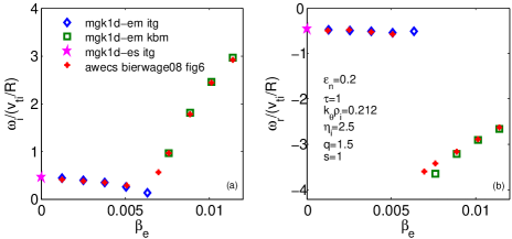
Figure 1: Benchmark of the eigenvalue solver MGK1d with particle code AWECS. Left and right frames show the imaginary ($\omega_{i}$) and real ($\omega_{r}$) parts of the eigenvalue divided by $v_{ti}/R$ respectively for different values of $\beta_{e}$. The blue diamonds and green squares indicate the ITG and KBM branches by solving Eqs. (II)-(II). The magenta pentagram indicates the electrostatic ITG branch with the constraint $\Psi=0$, which is tested in Xie2017 .

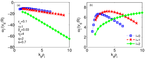
Figure 2: Left and right frames show the imaginary ($\omega_{i}$) and real ($\omega_{r}$) parts of the eigenvalue divided by $v_{ti}/R$ respectively for different values of $k_{\theta}\rho_{i}$. Different eigenstates of KBM co-exist, labeled with $l=0,1,2$. The $l=1$ KBM dominates for $3\lesssim k_{\theta}\rho_{i}\lesssim 7$, and the $l=2$ KBM dominates for $k_{\theta}\rho_{i}\gtrsim 7$.

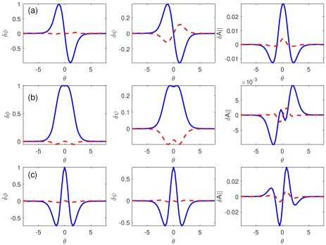
Figure 3: Mode structures of $\delta\phi$ (left), $\delta\psi$ (center) and $\delta A_{\parallel}$ (right) for the most unstable mode with $l=1$ and $\omega/(v_{ti}/R)=-17.2+7.04\imath$ (first row), the ground state mode (third most unstable) with $l=0$ and $\omega/(v_{ti}/R)=-14.5+5.31\imath$ (second row) and second most unstable mode with $l=2$ and $\omega/(v_{ti}/R)=-35.4+5.8\imath$ (third row) KBMs with $k_{\theta}\rho_{i}=5.0$. The blue solid line and the red dashed line indicate the real and imaginary parts of $\delta\phi$, $\delta\psi$ and $\delta A_{\parallel}$.

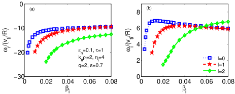
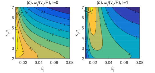
Figure 4: Beta scan for $l=0,1,2$ KBMs with $k_{\theta}\rho_{i}=2.0$ (a,b) and $(\beta_{i},k_{\theta}\rho_{i})$ scan for $l=0,1$ (c,d). Other parameters are the same as in Fig.2. At small $\beta_{i}$, all $l=0,1,2$ growth rates increasing with $\beta_{i}$ increasing, which is characteristic of KBM.

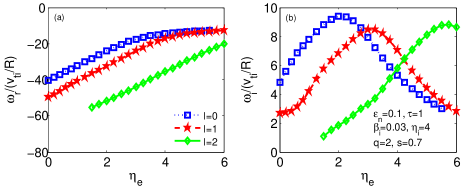
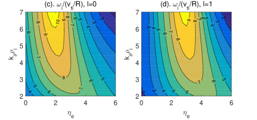
Figure 5: Scan of $\eta_{e}$ for $l=0,1,2$ (a,b) KBMs with $k_{\theta}\rho_{i}=5.0$ and $(\eta_{e},k_{\theta}\rho_{i})$ scan for $l=0,1$ (c,d). Other parameters are the same as in Fig.2. For $\eta_{e}=0$, the $l=0,1$ KBMs are still unstable, which means that electron temperature gradient is not a must for $l=1$ KBM.

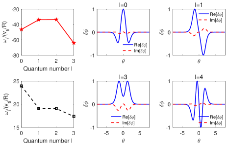
Figure 6: Left column of eigenvalues of $l=0,1,2,3$ for $\epsilon_{n}=0.05$, $\eta_{i}=8.5$, $k_{\theta}\rho_{i}=6.0$, $\beta_{i}=0.05$, $s=0.78$, $q=1.4$ and $\tau=1.0$. Central and right columns show the eigen functions.

III Results

We firstly benchmark our eigenvalue solver called MGK1d-EM which solves Eqs. (II)-(II) with the particle code AWECSBierwage2008 to repeat the conventional $l=0$ KBM. Figure 1 shows a $\beta_{e}$ scan of the complex frequency, where good agreement is obtained. The transition of the most unstable mode from electrostatic ITG to electromagnetic KBM is observed clearly. At $\beta\to 0$ limit, the present electromagnetic model can reproduce the electrostatic ITGs in Ref.Xie2017a as shown by the pink star in Fig.1. Hereafter, we will demonstrate our new result for high order eigenstates of KBM under steep gradient. Since Grad-Shafranov equilibrium with $\alpha=-2(Rq^{2}/B^{2})dp/dr$ is not valid for strong gradient, we will set $\alpha=0$, i.e., using concentric circles flux surface, to study the existence of high order KBMs. This leads to a shift of the critical condition of eigenstate transition and the detailed discussion of finite Grad-Shafranov shift will be discussed in a dedicated work. Note that our new high order modes are different from the “high order” KBM in Ref.Hirose1994 , which is still even parity of $\delta\phi$ but has broad mode structure. And also, the KBM in Ref.Hirose1994 is due to $\alpha$ potential well, as studied by Ref.Hu2004 , and called $\alpha$TAE. Thus, this is another reason we set $\alpha=0$, i.e., to remove the $\alpha$-induced potential well.

Typical cases under steep gradient analyzed in the following are characterized by $R/L_{Ti}=40$, where $L_{Ti}=1/(d\ln T_{i}/dr)$. Analyses based on more realistic experimental parameters are beyond the scope of this work. Figure 2 shows the co-existence of ground ($l=0$) and $l=1,2$ non-ground eigenstates for various $k_{\theta}\rho_{i}$ values. Unless explicitly indicated, other parameters in this work are $\epsilon_{n}=0.1$, $\tau=1$, $\beta_{i}=0.03$, $\eta_{i}=4$, $\eta_{e}=4$, $q=2$, $s=0.7$, $k_{\theta}\rho_{i}=5$. While the real frequency linearly scales with $k_{\theta}\rho_{i}$ for all eigenstates, the most unstable eigenstate is $l=0$ for $k_{\theta}\rho_{i}\lesssim 3$ and becomes $l=1$ for $3\lesssim k_{\theta}\rho_{i}\lesssim 7$ and $l=2$ for $k_{\theta}\rho_{i}\gtrsim 7$. The mode structures for $l=0,1,2$ are shown in Fig. 3 for $k_{\theta}\rho_{i}=5$. We identify the eigenstate number $l$ by roughly fitting the mode structure with the foregoing Weber equation solutions. The most unstable one is the non-ground eigenstate ($l=1$) with MTM parity. These are electromagnetic modes since $\psi/\phi\sim 0.3-0.6$ is not small. For electromagnetic ideal MHD mode with $E_{\parallel}\simeq 0$, we have $\delta\psi/\delta\phi\simeq 1$; and for electrostatic mode, we have $\delta\psi/\delta\phi\simeq 0$. We also notice that $\delta A_{\parallel}$ should have the opposite parity as that for $\delta\phi$ and $\delta\psi$ due to the derivative $\partial_{l}$ in the relation $\partial_{l_{\parallel}}\delta\psi=i\omega\delta A_{\parallel}$.

Figure 4 (a) shows that the absolute value of real frequency increases as $\beta_{i}$ increases for the $l=0,1,2$ eigen states. Figure 4 (b) shows the growth rate $\omega_{i}$ of all eigenstate increases with $\beta_{i}$ at small $\beta_{i}$. However, when $\beta_{i}$ is above a critical value, $\omega_{i}$ of the ground ($l=0$) state decreases as $\beta_{i}$ increases and the non-ground eigenstate can have larger $\omega_{i}$ than the ground state. Figure 4 (c) and (d) show the growth rate of the ground and excited eigenstates in $(\beta_{i},k_{\theta}\rho_{i})$ space. The ground and excited eigenstates can co-exist in general and for the parameters concerned here, as $\beta_{i}$ increases, the dominant instability transits from the ground state to the excited state and the spectrum shifts from $k_{\theta}\rho_{i}\sim 3$ to $k_{\theta}\rho_{i}>7$.

It is generally believed that MTM with odd mode parity is driven by electron temperature gradient Hazeltine1975 ; Applegate2007 ; Dickinson2012 ; Moradi2013 ; Chowdhury2016 , i.e., requiring $\eta_{e}\neq 0$. Here, we show that the excited ($l\neq 0$) state of KBM is unstable under steep gradient even with $\eta_{e}=0$ and thus is different than the MTM. The dependence of eigenvalue on $\eta_{e}$ is shown in Fig. 5 (a) and (b). The fixed ion temperature gradient $\eta_{i}=4$ drives the ground (dominant) and non-ground states even $\eta_{e}=0$. As $\eta_{e}$ increases, similar to the $\beta_{i}$ dependence, the most unstable eigenstate changes from $l=0$ to $l=1$. For $\eta_{e}=0$, the $l=0,1$ KBMs are still unstable, which indicates that electron temperature gradient is not the only unstable mechanism for $l=1$ KBM. The most unstable eigenstate can shift from $l=0$ to $l=1$ depending on the strength of the drive such as $\beta_{i}$ and $\eta_{e}$. The co-existence of the even and odd parity eigenstates in $(\eta_{e},k_{\theta}\rho_{i})$ space is shown in Fig. 5 (c) and (d), where the different eigenstates have comparable growth rate in the whole parameter regime. Also note that the model we used is collisionless, thus the $l\geq 1$ KBMs can become unstable without collision. For even stronger drive, with $\epsilon_{n}=0.05$, $\eta_{i}=8.5$, $k_{\theta}\rho_{i}=6.0$, $\beta_{i}=0.05$, $s=0.78$, $q=1.4$ and $\tau=1.0$, the unstable $l=3$ KBM is also found, as shown in Fig. 6. This indicates that indeed series high order eigenstates of KBM exist and they can be unstable easily or even be the most unstable eigenstate under strong gradient.

In mathematical aspect, the existence of high order eigenstates is not surprising, especially for slab geometryPearlstein1969 . Electrostatic high order drift modes in tokamak such as ITGs (ion temperature gradient mode) and TEMs (trapped electron mode) have been found to be important at strong gradient edge parameters recently, both linearly Xie2015 ; Xie2016 and nonlinearly Xie2017 . The existence of $l=1$ AITG (Alfvénic ITG) in slab geometry without curvature drift has been reported in Refs.Reynders1992 and Gao2002 . This $l=1$ mode is called MTM by Reynders Reynders1992 and called tearing parity AITG by Gao et al Gao2002 . The $l\geq 2$ modes are considered to be stable in their slab study. For electrostatic case in the narrow parallel mode structure limit (strong ballooning approximation), we have a Weber equation for the mode structure (cf. Xie2015 ), $({d^{2}}/{d\theta^{2}}+\nu-c^{2}\theta^{2})\delta\phi(\theta)=0$, where $\nu=\nu(\omega)$, $c=c(\omega)$ and $\theta$ is the coordinate along a field line. The eigenvalue and eigenfunction are $D_{l}\equiv\nu-(2l+1)c=0$ an $\delta\phi=H_{l}(\sqrt{c}\theta)e^{-c\theta^{2}/2}$, where $H_{l}$ are $l$-th order Hermite polynomials, with $l=0,1,2,\cdots$. The subscript $l$ represents the quantum number and even/odd $l$ correspond to even/odd mode parity respectively. This implies that the high order KBMs can exist, and they can be ubiquitous under edge steep gradient parameters. This intuitive picture based on the Weber equation provides a way to understand the more complicated model for which a series of KBM high order states can exist and the even parity states can be more unstable depending on the parameters.

We note that the quantitative solutions will be affected by the electromagnetic models, e.g., with trapped particle, non-adiabatic electron, finite $\delta B_{\parallel}$ and global effects. For examples, the existence conditions and parameter dependence could be different from the above results if additional effects are included. However, the general conclusion can be listed as follows: (1) Unstable higher order $l\geq 1$ KBMs exist and can be dominant at strong gradient; (2) even and odd mode structure parities are connected to different eigenstates; (3) The pressure gradient is a sufficient condition for the destabilization of higher order KBMs, even without collision, kinetic electron and electron temperature gradient as demonstrated in our results.

IV Conclusions

In summary, we have demonstrated the existence of unstable high order KBMs. It merits more effort to study the excited eigenstates of KBMs in fusion experiments, especially under strong gradient edge plasma parameters. Our previous works Xie2015 only considered electrostatic case. In this work, we conclude that both electrostatic and electromagnetic non-ground eigenstates can be important or even dominant at the strong gradient plasma edge. Since these various dominant Xie2017 and subdominant Hatch2013 electrostatic and electromagnetic eigenstates can affect the nonlinear physics at the same time, the edge plasma physics can be extremely complicated, which can explain why the edge physics is very different and complicated than that in the core plasma. We expect that this picture of various eigenstates can shed light on the KBM study for steep gradient profiles, which is relevant to the edge electromagnetic microinstabilities and consequent nonlinear physics including turbulent transport. The eigenmode parity could be also important for other physics, such as parallel momentum transport Diamond2013 and energetic particles driven Alfvén eigenmodes (AE) Chen2016 ; Lauber2005 , and different parity AEs have indeed been observed experimentallyKramer2004 . And thus, the extension of this work to other topics such as Alfvén eigenmode and momentum transport is also expected to introduce new insight.

Acknowledgments.– HSX would like to thank Yue-Yan Li, Jian Bao, David Hatch and Fulvio Zonca for fruitful discussions. This work was supported by the China Postdoctoral Science Foundation No. 2016M590008, Natural Science Foundation of China under Grant No. 11675007 and 11605186, and the ITER-China Grant No. 2013GB112006.

References

- (1) T. S. Hahm, Plasma Phys. Control. Fusion, 44, A87 (2002).
- (2) F. Wagner, Plasma Phys. Control. Fusion, 49, B1 (2007).
- (3) H. S. Xie, Y. Xiao and Z. Lin, Phys. Rev. Lett., 118, 095001 (2017).
- (4) C. S. Chang, S. Ku, G. R. Tynan, R. Hager, R. M. Churchill, I. Cziegler, M. Greenwald, A. E. Hubbard, and J. W. Hughes, Phys. Rev. Lett., 118, 175001 (2017).
- (5) J. W. Connor, R. J. Hastie and J. B. Taylor, Phys. Rev. Lett., 40, (1978).
- (6) W. Tang, J. Connor and R. Hastie, Nucl. Fusion, 20, 1439 (1980).
- (7) P. B. Snyder R. J. Groebner, A.W. Leonard, T. H. Osborne, and H. R. Wilson, Phys. Plasmas 16, 056118 (2009).
- (8) D. Dickinson, C. M. Roach, S. Saarelma, R. Scannell, A. Kirk and H. R. Wilson, Phys. Rev. Lett., 108, 135002 (2012).
- (9) W. Wan, S. E. Parker, Y. Chen, Z. Yan, R. J. Groebner and P. B. Snyder, Phys. Rev. Lett., 109, 185004 (2012).
- (10) R. D. Hazeltine, D. Dobrott, and T. S. Wang, Phys. Fluids 18, 1778 (1975).
- (11) J. W. Connor, S. C. Cowley, and R. J. Hastie, Plasma Phys. Control. Fusion 32, 799 (1990).
- (12) D. J. Applegate, C. M. Roach, J. W. Connor, S. C. Cowley, W. Dorland, R. J. Hastie and N. Joiner, Plasma Phys. Control. Fusion, 49 1113 (2007).
- (13) W. Guttenfelder, J. Candy, S. M. Kaye, W. M. Nevins, E. Wang, R. E. Bell, G. W. Hammett, B. P. LeBlanc, D. R. Mikkelsen, and H. Yuh, Phys. Rev. Lett. 106, 155004 (2011).
- (14) M. Zuin, S. Spagnolo, I. Predebon, F. Sattin, F. Auriemma, R. Cavazzana, A. Fassina, E. Martines, R. Paccagnella, M. Spolaore, and N. Vianello, Phys. Rev. Lett., 110, 055002 (2013).
- (15) S. Moradi, I. Pusztai, W. Guttenfelder, T. Fülöp and A. Mollén. Nucl. Fusion 53 063025 (2013).
- (16) J. Chowdhury, Y. Chen, W. Wan, S. E. Parker, W. Guttenfelder and J. M. Canik, Phys. Plasmas, 23, 012513 (2016).
- (17) D. Hatch, M. Kotschenreuther, S. Mahajan, P. Valanju, F. Jenko, D. Told, T. Görler and S. Saarelma, Nucl. Fusion, 56, 104003 (2016).
- (18) E. Hameiri, P. Laurence and M. Mond, Journal of Geophysical Research: Space Physics, 96, 1513 (1991).
- (19) P. H. Diamond, Y. Kosuga, Ö.D. Gürcan, C.J. McDevitt, T.S. Hahm, N. Fedorczak, J.E. Rice, W.X. Wang, S. Ku, J.M. Kwon, Nucl. Fusion, 53, 104019 (2013).
- (20) C. Angioni, Y. Camenen, F.J. Casson, E. Fable, R. M. McDermott, A.G. Peeters, and J.E. Rice, Nucl. Fusion, 52, 114003 (2012)
- (21) L. Chen and F. Zonca, Rev. Mod. Phys., 88, 015008 (2016).
- (22) H. Doerk, F. Jenko, M. J. Pueschel and D. R. Hatch, Phys. Rev. Lett., 106, 155003 (2011).
- (23) A. K. Swamy, R. Ganesh, J. Chowdhury, S. Brunner, J. Vaclavik, and L. Villard, Phys. Plasmas, 21, 082513 (2014).
- (24) H. P. Furth, J. Killeen and M. N. Rosenbluth, Phys. Fluids, 6, 459 (1963).
- (25) L. D. Pearlstein and H. L. Berk, Phys. Rev. Lett. 23, 220 (1969).
- (26) H. S. Xie and Y. Xiao, Phys. Plasmas, 22, 090703 (2015);
- (27) H. S. Xie and B. Li, Phys. Plasmas, 23, 082513 (2016).
- (28) J. V. M. Reynders, PhD thesis, Princeton University, 1992.
- (29) Z. Gao, J. Q. Dong, G. J. Liu and C. T. Ying, Phys. Plasmas, 9, 1692 (2002).
- (30) A. J. Brizard and T. S. Hahm, Rev. Mod. Phys., 79, 421 (2007).
- (31) L. Chen and A. Hasegawa, Journal of Geophysical Research, 96, 1503 (1991).
- (32) H. S. Xie, Y. Y. Li, Z. X. Lu, W. K. Ou and B. Li, Phys. Plasmas, 24, 072106 (2017).
- (33) A. Bierwage and L. Chen, Commun. Comput. Phys., 4, 457 (2008).
- (34) A. Hirose, L. Zhang and M. Elia, Phys. Rev. Lett., 72, 3993 (1994).
- (35) S. Hu and L. Chen, Phys. Plasmas, 11, 1 (2004). (2005).
- (36) D. R. Hatch, M. J. Pueschel, F. Jenko, W. M. Nevins, P. W. Terry, and H. Doerk, Phys. Plasmas, 20, 012307 (2013).
- (37) Ph. Lauber, S. Günter and S. D. Pinches, Phys. Plasmas, 12, 122501 (2005).
- (38) G. J. Kramer, S. E. Sharapov, R. Nazikian, N. N. Gorelenkov and R. V. Budny, Phys. Rev. Lett. 92, 015001 (2004).