Search for quasi-periodic signals in magnetar giant flares

Quasi-periodic oscillations (QPOs) discovered in the decaying tails of giant flares of magnetars are believed to be torsional oscillations of neutron stars. These QPOs have a high potential to constrain properties of high-density matter. In search for quasi-periodic signals, we study the light curves of the giant flares of SGR 1806-20 and SGR 1900+14, with a non-parametric Bayesian signal inference method called D³PO. The D³PO algorithm models the raw photon counts as a continuous flux and takes the Poissonian shot noise as well as all instrument effects into account. It reconstructs the logarithmic flux and its power spectrum from the data. Using this fully noise-aware method, we do not confirm previously reported frequency lines at $\nu\gtrsim 17\,$Hz because they fall into the noise-dominated regime. However, we find two new potential candidates for oscillations at $9.2\,$Hz (SGR 1806-20) and $7.7\,$Hz (SGR 1900+14). If these are real and the fundamental magneto-elastic oscillations of the magnetars, current theoretical models would favour relatively weak magnetic fields $\bar{B}\sim 6\times 10^{13}-3\times 10^{14}\,$G (SGR 1806-20) and a relatively low shear velocity inside the crust compared to previous findings.

1 Introduction

The discovery of quasi-periodic oscillations (QPOs) in the giant flare of the magnetar SGR 1806-20 by Israel et al. (2005) may have been the first detection of neutron star oscillations and triggered a wealth of theoretical work explaining the reported frequencies. The giant flare was likely caused by a large-scale reconnection or an interchange instability of the magnetic field (Thompson & Duncan 1995). Large amounts of energy are released as an expanding $e^{\pm}$-pair plasma, observable as the initial spike of the giant flare. Parts of this plasma are trapped by the ultra-strong magnetic field and form a so-called trapped fireball (Thompson & Duncan 1995), which then slowly evaporates on a timescale of up to a few $100$ seconds. The QPOs were detected in this decaying tail of the giant flare. Other groups have not only confirmed this detection, they even found additional oscillation frequencies in different magnetars: $18$, $26$, $29$, $92$, $150$ , $625$, and $1840$ Hz in the giant flare of SGR 1806-20, and $28$, $53$, $84$, and $155$ Hz in the giant flare of SGR 1900+14 (e.g. Strohmayer & Watts 2005; Watts & Strohmayer 2006; Strohmayer & Watts 2006; Huppenkothen et al. 2014c). With different methods, more oscillation frequencies were found in the giant flare of SGR 1806-20 by Hambaryan et al. (2011) $17$, $21$, $36$, $59$, and $116\,$Hz. The number of giant flares at the time of writing is limited to three events. The more frequent but less energetic bursts of several magnetars have therefore also been investigated for frequencies, and some candidates were found: $57\,$Hz in SGR 1806-20 (Huppenkothen et al. 2014b), and at $93$, $127$, and $260\,$Hz in SGR J1550-5418 (Huppenkothen et al. 2014a).

It was soon realized that these frequencies are probably related to oscillations of the neutron star, and several groups tried to identify them as elastic oscillations of the crust (Duncan 1998; Messios et al. 2001; Strohmayer & Watts 2005; Piro 2005; Sotani et al. 2007; Samuelsson & Andersson 2007; Steiner & Watts 2009; Samuelsson & Andersson 2009; Sotani et al. 2013; Deibel et al. 2014; Sotani et al. 2016), Alfvén oscillations (Cerdá-Durán et al. 2009; Sotani et al. 2008; Colaiuda et al. 2009), or coupled magneto-elastic oscillations (Levin 2006, 2007; Glampedakis et al. 2006; Gabler et al. 2011, 2012; Colaiuda & Kokkotas 2011; van Hoven & Levin 2011, 2012). The theoretical models based on the observed frequencies are very elaborate and may be able to constrain properties of high-density matter as found in the interior of neutron stars. Some of the models, for instance, require a superfluid component in the core of the star (van Hoven & Levin 2011, 2012; Glampedakis et al. 2011; Passamonti & Lander 2013; Gabler et al. 2013; Passamonti & Lander 2014; Gabler et al. 2016, 2017). Different models depend sensitively on the identification of the fundamental oscillation frequency, and may not explain all of the observed frequencies. Even when the fundamental frequency is identified, the interpretation and parameter estimation is not yet straightforward because of degeneracies in the parameter space. However, keeping other stellar parameters fixed, some general trends of the fundamental oscillation frequency can be summarized as follows (see Gabler et al. 2016, 2017, for a detailed discussion): i) The frequency scales linearly with the magnetic field strength. ii) It decreases with increasing compactness (Sotani et al. 2008). The compactness is related to the hardness of the equation of state (EOS): Material with a stiff equation of state is harder to compress, leading to larger radii and hence lower compactnesses. iii) It can only reach the surface for significantly strong magnetic fields $\bar{B}\gtrsim\bar{B}_{\text{outbreak}}(\sqrt{c_{s}})$, whose thresholds depend on the square root of the shear velocity (Gabler et al. 2017).

It is of great importance to understand which of the frequencies are in the signal. In previous attempts at identifying possible frequencies in the light curve, the statistical noise of the detectors was not modelled consistently. To improve on this, we employ a Bayesian method that properly takes the photon shot noise as the largest contributor into account.

In this work, we re-analyse the data for the two giant flares of SGR1806-20 and SGR1900+14, which were obtained with the proportional counter array (PCA) of the Rossi X-ray Timing Explorer (RXTE). The data are available online at the High Energy Astrophysics Science Archive Research Center (HEASARC). In Section 2 we briefly discuss our numerical approach to estimating the influence of the noise and to reconstructing the likely signal with a reduced contribution from the noise. The next section is devoted to the reconstruction and investigation of the light curves of the two giant flares of SGR 1806-20 and SGR 1900+14, which are then discussed in Section 4. We conclude our analysis in Section 5.

2 Inference of photon observations

Our goal is to reconstruct the light curve and possible frequencies of QPOs in giant X-ray flares for the neutron stars SGR 1806-20 and SGR 1900+14 using the data taken by RXTE. Owing to experimental constraints such as limited data storage, finite time resolution of each photon count, finite detector size, and sensitivity, RXTE cannot record all physical relevant and available information of a continuous photon flux. Most importantly, the recorded photon counts contain significant photon shot noise. Hence, we have to use probabilisitic data analysis methods to obtain an estimate of the time-dependent, continuous photon flux $\@vec{\phi}\left(t\right)$ , including its uncertainties. Since the flux varies on a logarithmic scale, we reconstructed the logarithm of the flux $s\left(t\right)=\log\left(\@vec{\phi}\left(t\right)/\phi_{0}\right)$ and its temporal power spectrum directly from the data.

In this context, it is natural to build the inference upon the Bayes theorem, allowing us to investigate the a posteriori probability distribution $P\left(\@vec{\phi}|\@vec{d}\right)$, stating how likely a given photon flux field $\@vec{\phi}$ is given the data set $\@vec{d}$ . For the two data sets of SGR 1806-20 and SGR 1900-14, we assumed the data $\@vec{d}$ to be the result of a Poisson process whose expectation value $\@vec{\lambda}$ is given by the photon flux $\@vec{\phi}\left(t\right)$ of the photon burst convolved with the response operator $\@vec{R}$,

$$\@vec{\lambda}=\@vec{R}\@vec{\phi}\left(t\right)=\@vec{R}\phi_{0}e^{s\left(t\right)}\,.$$ (1)

The response operator encodes all instrument specifications and states how $\@vec{\phi}$ imprints itself on $\@vec{\lambda}$. Here, we only considered the readout deadtime periods of the instrument and neglected all other instrument responses. In Equation 1 the constant $\phi_{0}$ absorbs numerical constants and the physical units of the time dependent log- flux signal field $s\left(t\right)=\@vec{s}$. As the signal describes the logarithmic flux, we naturally ensured the positive definiteness of the photon flux. Since we analysed QPOs, it is expected that $\@vec{\phi}$ exhibits unknown but spatial correlations. Hence, we did not enforce any concrete spatial correlations. We only assumed $\@vec{\phi}$ to follow a multivariate log-normal statistic, with an a priori unknown covariance. Assuming stationary statistics, the underlying covariance is fully determined by a power spectrum $P_{s}\left(\nu\right)$, described by $P_{s}\left(\nu\right)=P_{0}e^{\@vec{\tau}\left(\nu\right)}$, to ensure positivity of the power spectrum. We inferred this power spectrum as well as $\@vec{\phi}$ from the data themselves by setting up a hierarchical prior model (Selig et al. 2015; Junklewitz et al. 2016; Pumpe et al. 2016; Enßlin & Frommert 2011; Enßlin & Knollmüller 2016). Hence the posterior of our Bayesian inference is given by

$$P\left(\@vec{\phi},\@vec{\tau}|\@vec{d}\right) \propto\frac{P\left(,\@vec{d}|\@vec{\phi},\@vec{\tau}\right)P\left(\@vec{\tau}|\sigma_{\mathrm{sm}}\right)}{P\left(\@vec{d}\right)}\,,$$ (2)

where $P\left(\@vec{d}|\@vec{\phi},\@vec{\tau}\right)$ is the likelihood describing how a potential photon flux $\@vec{\phi}$ including a certain covariance structure described by $\@vec{\tau}$ imprints itself in a potential data set. In addition to strong spectral peaks in the power spectrum induced by the almost discrete frequencies of QPOs, we enforce some kind of spectral smoothness on the logarithmic scale, favouring power-law spectra. This behaviour is enforced and tuned by the prior term $P\left(\@vec{\tau}|\sigma_{\mathrm{sm}}\right)$ and its parameter $\sigma_{\mathrm{sm}}$ (Oppermann et al. (2013)). If $\sigma_{\mathrm{sm}}\rightarrow 0,$ infinite spectral smoothness is enforced, while $\sigma_{\mathrm{sm}}\rightarrow\infty$ does not enforce any spectral smoothness. As we wish to be sensitive to spectral lines in the power spectrum, the influence of $\sigma_{\mathrm{sm}}$ on the inference is discussed in greater detail in Appendix A.

For the detailed mathematical rigorous derivation and discussion of the used D³PO- algorithm, we refer to Selig & Enßlin (2015) and Enßlin & Knollmüller (2016). The D³PO- algorithm was successfully applied on the Fermi LAT data (Selig et al. 2015). In order to handle high power spectrum resolutions as is needed to infer spectral lines in the power spectrum, we reimplemented the algorithm in NIFTy 3 (Steininger et al. 2017). The capabilities of the algorithm to analyse QPOs are demonstrated in the Appendices A, B and C.

3 Results

3.1 SGR 1806-20

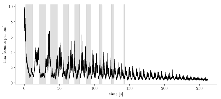
We re-analysed the archival RXTE data of the giant flare of SGR 1806-20, which occurred on 2004 December 27. Owing to the high photon flux, the instrument telemetry was saturated, causing several data gaps in the first seconds of the flare. We therefore neglected the very beginning of the flare in the current analysis and started our investigation roughly $4.5\,$s after the initial rise, immediately after the third deadtime interval. However, we accounted for the only remaining operational down time of the instrument in our data between $7.3865\,\text{s}\leq\text{t}\leq 7.9975\,\text{s}$. For the analysis, we binned the data into pixels with a volume of $1/800\,$s. To overcome the periodic boundary conditions introduced by the fast-Fourier transformation, which we used to switch between signal space and its harmonic space, we performed the signal inference on a regular grid with $2^{19}$ pixel, each also with a volume of $1/800\,$s, by adding sufficient buffer time.

(a)

(b)

Figure 1: Reconstructed light curve of the giant flare of SGR 1806-20 using a smoothness-enforcing prior, with $\sigma_{\mathrm{sm}}=5\times 10^{5}$ is shown in Figure 1(a). The grey narrow rectangle indicates the operational down time of the instrument. For better visibility, we plot the light curve between $\approx 164\,$s and $\approx 174\,$s in Figure 1(b). In addition to the raw photon counts (black dots), the black line indicates the reconstruction of the expected photon counts, i.e. $\lambda$ as well as its one-$\sigma$ confidence interval. Owing to the high resolution of the photon flux, only every fourth point of the regular grid is plotted. In both plots each pixel has a duration of $1/800\,$s .

Figure 2: Pulse profiles of different rotation periods overplotted as given in Figure 1(a). The temporal evolution of the pulse profile is visible from blue to green to red. The mean pulse is shown as a thick black line. All pulses are shifted such that their log-means are zero.

(a)

(b)

(c)

Figure 3: Reconstructed power spectra of the giant flare of SGR 1806-20: For Figure 3(a) and Figure 3(c) we used smoothness-enforcing priors with $\sigma_{\mathrm{sm}}=5\times 10^{5}$ and $\sigma_{\mathrm{sm}}=10^{5}$, respectively. The uncertainty intervals are given as grey shaded areas. In Figure 3(b) we show the reconstructed power spectrum again from the data themselves as in Figure 3(a), along with the power spectrum of the logarithmic reconstructed light curve of Figure 1(a). Because of the high resolution of the reconstructed power spectra, only every fourth point of the regular grid is plotted. Each pixel has a volume of $1/655\,$Hz.

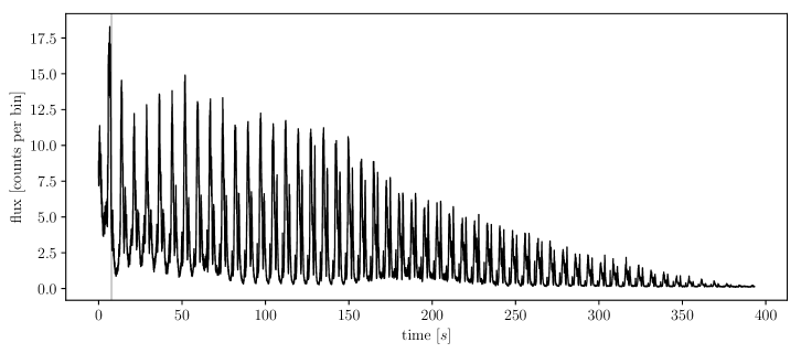
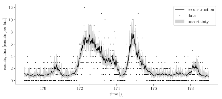
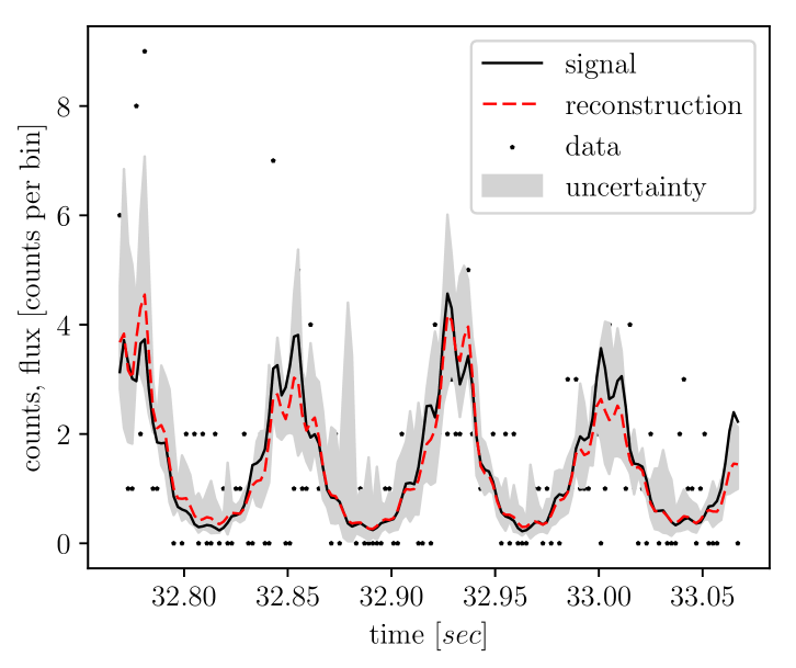
In Figure 1 we plot the inferred $\@vec{\phi}$ for the entire duration of the giant flare and for a selected period of time for a smoothness parameter $\sigma_{\mathrm{sm}}=5\times 10^{5}$. Our algorithm is able to significantly reduce the scatter of the light curve that is caused by the photon shot noise. The thus reconstructed light curves can now be further analysed for potential periodic signals.

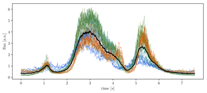
Figure 2 shows the reconstructed profiles of one pulse rotation period. There, the mean pulse profile is given as a thick black line, and all individual pulses are plotted in different colours. Dark blue are the first pulses that have a significantly lower second maxima around $5.5\,$s than the mean pulse. The major maximum ($\mathrm{time}\sim 3\,$s) is very close to the mean maximum. At intermediate times (green lines), both maxima of the pulse take their maximum values, roughly $40\%$ and $130\%$ more than at the beginning for the first and second maximum, respectively. At late times (red lines) the main peak declines by $40\%,$ while the second maximum almost stays constant and has an amplitude similar to the main peak. This behaviour indicates a complex evolution of the fireball, or of the fireballs, if there are more than one.

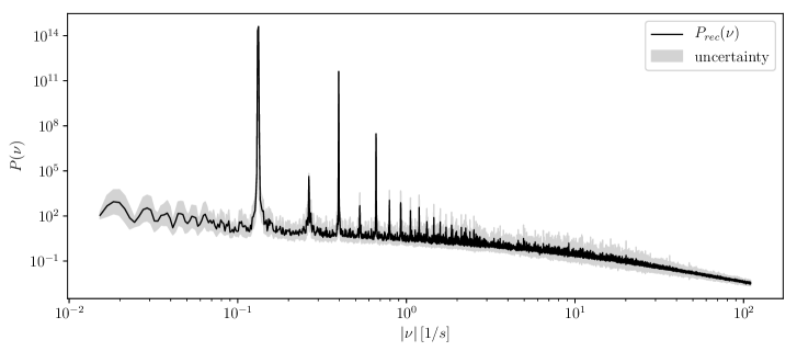
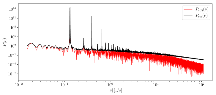
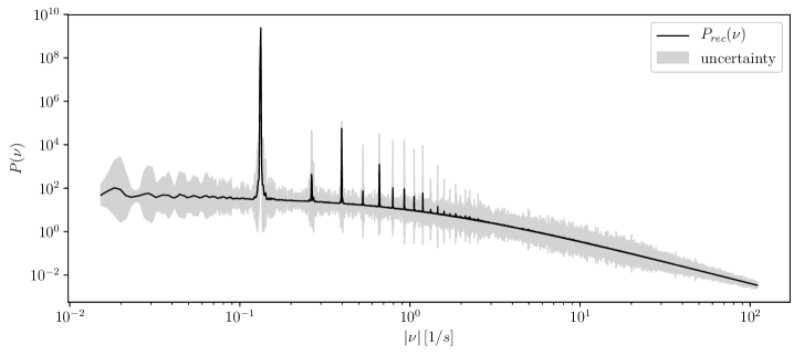
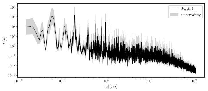
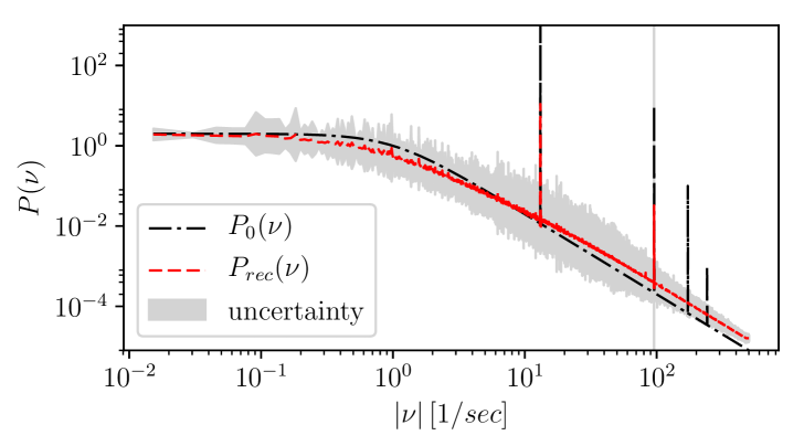
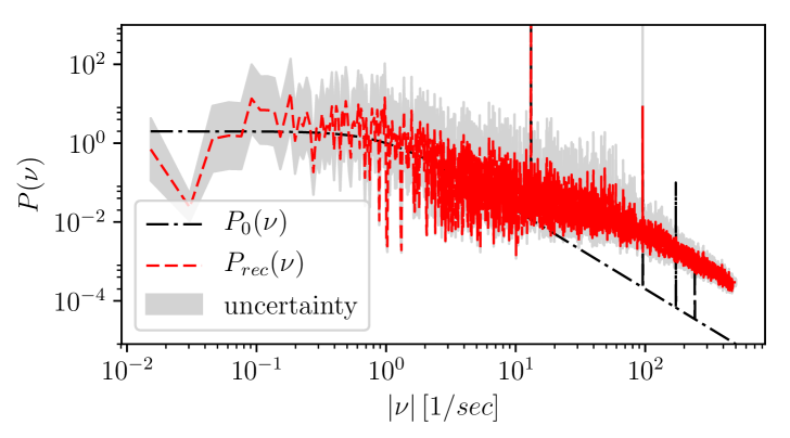
The power spectrum of the entire flare is plotted in Figure 3(a). The rotation period of the magnetar is recovered with the frequency of the first main peak $\nu_{0}=0.1323\,$Hz, which is very close to $\nu_{0}=0.13249\,$Hz, as given in Olausen & Kaspi (2014). We are able to find up to the $31$st overtone of this frequency at $\nu=4.245\,$Hz. In Figure 3(b) we show the reconstructed power spectrum $P_{\text{rec}}$ from Figure 3(a) in black together with the power spectrum obtained from the reconstructed light curve (Figure 1(a)) $P_{s\left(t\right)}\left(\nu\right)$ in red. At low frequencies, that is, $\nu\lesssim 3\,$[Hz], the two spectra are in good agreement, as the reconstruction is well constrained by the data on large scales. Between $3\,\text{[Hz]}\lesssim\nu\lesssim 20\,\text{[Hz]}$, the inference algorithm enters the regime of a lower signal-to-noise ratio (S/N), which in principle leads to noisier $P_{\mathrm{rec}}$. However, this natural behaviour is counteracted by the smoothness-enforcing prior. At higher $\nu\gtrsim 20$ Hz, the shapes of both spectra start to deviate significantly. The reason for this is that in the noise-dominated frequency regime, D³PO filters out the photon shot noise. From a naive perspective, small-scale features in the signal therefore need to be significantly strong in order to be detectable after a pure photon shot noise filtering operation on the data set. However, D³PO accounts for the power loss of this filtering when it reconstructs the power spectrum from the data themselves. Thus, Figure 3(b) indicates that above $20$ Hz the data are noise dominated, and spectral features there have to be very strong to be recognisable. To test the dependence of our method on the chosen smoothness prior $\sigma_{\mathrm{sm}}$ as discussed also in Appendix A, we additionally calculated the reconstructed light curve and its corresponding power spectrum for $\sigma_{\mathrm{sm}}=10^{5}$. The latter is given in Figure 3(c). Obviously, a smaller $\sigma_{\mathrm{sm}}$ leads to a smoothing of the spectrum and the algorithm suppresses the detection of periodic signals at higher frequencies. We found $\sigma_{\mathrm{sm}}=5\times 10^{5}$ to be the optimal value to still observe power in the Fourier transform at higher frequencies. For higher values of $\sigma_{\mathrm{sm}}$ , we qualitatively obtain similar but more noisy results for the reconstructed light curve and the corresponding power spectra.

In addition to the obvious peaks that are related to the rotation period and the corresponding overtones, there are still other features in the reconstructed power spectrum of Figure 3(a) that seem to have higher powers than the noise. To estimate the significance of these spectral peaks, we calculated a residual $\chi$ between the inferred log-spectrum $\tau$ and its local median $\bar{\tau}$ weighted with the local variance $\sigma$,

$$\chi=\frac{\tau-\bar{\tau}}{\sigma}\,.$$ (3)

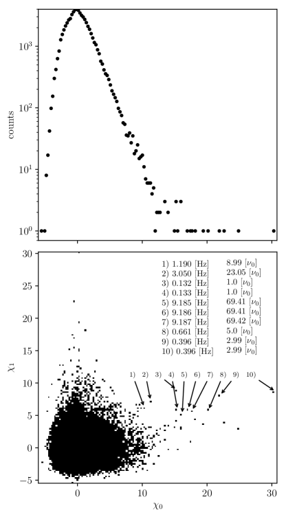
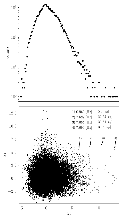
The local median and local variance were calculated over a window of $401$ pixels, corresponding to a frequency window of approximately $1\,$Hz. In the top panel of Figure 5 we plot the histogram of $\chi_{0}$, where the index $0$ refers to the fundamental frequency, that is, $\chi$ at the respective frequency. The resulting distribution deviates significantly from a Gaussian, as there is a significant excess for large $\chi_{0}$. These counts can easily be identified with the highest spectral peaks in Figure 3(a) as integer multiples of the neutron star rotation frequency of $\nu_{0}=0.1323\,$Hz. The fat tails of the distribution make it hard to identify whether a peak sticks out of the tail, in particular for $\chi_{0}\gtrsim 10$. For $\chi_{0}\gtrsim 15$ all peaks can be identified and are related to the neutron star rotation period, except for one at $\nu\sim 9.187\,$Hz. In Table 1 we show all frequencies that have $\chi_{0}>11$ to have a selection of possible oscillation candidates. If there are two or more neighbouring frequencies with $\chi_{0}>11$, we list the highest value.

Table 1: All frequencies above $3.5\,$Hz with $\chi_{0}>11$ and their multiplicity $n$ of the rotation period $\nu_{0}=0.13249$ [Hz] for SGR 1806-20.

$\nu$ [Hz]	$\chi_{0}$	$n$ [$\nu_{0}$]	$\nu$ [Hz]	$\chi_{0}$	$n$ [$\nu_{0}$]
3.86	11.071	29.134	11.171	11.762	84.316
4.602	11.141	34.735	15.768	11.999	119.013
4.95	13.592	37.361	16.272	12.772	122.817
6.81	11.212	51.4	19.034	12.632	143.664
9.187	18.293	69.341

All other candidates in Table 1 have significantly lower $\chi$ than the oscillation at $9.187\,$Hz and are consistent with being in the tail of the distribution that is shown in the top panel of Figure 5. This indicates that these are artefacts of the Poisson noise.

Table 2: Maximum $\chi_{0}$ at $\nu_{\text{max}}$ in a $5\%$ interval around previously observed oscillation frequencies $\nu$ for SGR 1806-20. We also show the local variance $\sigma_{\chi}$ of $\chi_{0}$ at this interval.

$\nu$ [Hz]	$\nu_{\text{max}}\,$[Hz] in $\pm 5\%$ interval	$\chi_{0,\text{max}}$	$\sigma_{\chi}$
16.9	16.27	12.772	6.623
18.0	18.265	10.789	5.229
21.4	20.609	9.191	4.194
26.0	26.686	8.709	3.917
29.0	28.87	7.121	3.234
36.8	36.412	8.565	2.82
59.0	56.592	5.146	2.258
61.3	63.162	5.027	2.114
92.5	90.364	4.699	1.859
116.3	118.346	4.363	1.817
150	152.252	4.316	1.675

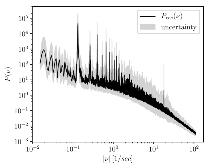
We also checked the $\chi_{0}$ values of previously reported frequencies. None of them reach more than $\chi_{0}\gtrsim 5$. We therefor extended our search in a $\pm 5\%$ interval around the frequencies in Table 2. The only frequency higher than $\chi_{0}=11$ is at $\nu=16.27\,$Hz. Thus all reported lines are consistent with noise. However, we already see an interesting pattern emerging: In Table 2 we locally (within the $\pm 5\%$ interval) find the highest powers at $18.265$ and $36.412\,$Hz. These are almost twice and four times the only significant frequency at $\nu=9.187\,$Hz that our method detects beyond the rotational frequency and its first 31 harmonics. In Figure 4 we plot the reconstructed power spectrum around the $\nu=9.187$ Hz candidate oscillation (black line) and its first overtone (red line). The amplitude at $\nu=9.187$ Hz is significantly larger (factor 2) than other amplitudes in the shown frequency range, while the amplitude at $\nu=18.265\,$Hz is comparable with other spectral peaks. As discrete frequencies in a power spectrum are likely to show spectral peaks at integer multiplies of a ground frequency, we also display the two-dimensional histogram of the calculated weighted residual $\chi_{0}$ at some ground frequency on the x-axis and its first harmonics $\chi_{1}$ on the y-axis in the bottom panel of Figure 5. We marked all counts with $\chi_{1}\geq 5$ and $\chi_{0}\geq 10$ with their corresponding frequency in Hz. We find about ten frequencies that satisfy this criterium. Obviously, all but the frequencies around $\nu\sim 9.186\,$Hz are integer multiples of the rotation frequency $\nu_{0}$.

Figure 4: Zoomed-in view of the reconstructed power spectra of giant flare SGR 1806-20 around $\nu\sim 9.186\,$Hz in black and its first overtone around $\nu\sim 18.265\,$Hz in red. The spectra correspond to $\sigma_{\mathrm{sm}}=5\times 10^{5}$ as in fig. 3(a)

Figure 5: Top panel: Histogram of the residuals between the logarithmic power spectrum of Figure 3(a) and its local median, weighted with its local variance $\sigma$. Bottom panel: Two-dimensional histogram of the same quantity at some frequency at the x-axis and its first harmonic at the y-axis. In addition, we indicate for all counts with $\chi_{1}\geq 5$ and $\chi_{0}\geq 10$ the corresponding frequency in Hertz and its multiple of the neutron star frequency, $\nu_{0}=0.1323\,$Hz. To generate the histograms, we used the power spectrum shown in Figure 3(a), i.e. $\sigma=5\times 10^{5}$.

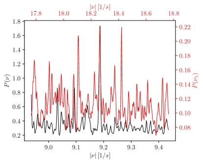
This further increases our confidence that $\nu\sim 9.186\,$Hz is a candidate for an additional periodic signal in the data. We do not find any significant features for frequencies higher than the corresponding overtones that the algorithm recovered at $\nu\sim 18.265\,$Hz and $\nu\sim 36.412\,$Hz.

3.2 SGR 1900+14

Analogously to SGR 1806-20, we also re-analysed the archival RXTE data of the giant flare of SGR 1900+14 that occurred on 1998 August 27. The resolution of the signal field is again $1/800\,$s, but here we only used $2^{18}$ pixels, as the giant flare did not last as long as that of SGR 1806-20. The operational down times of RXTE during the observation were taken into account for the inference.

(a)

(b)

(c)

(a)

Figure 7: Figure 6(a) shows the reconstructed light curve $\@vec{\phi}$ for SGR 1900+14. The grey rectangles indicate the operational down times of the instrument. Figure 6(b) shows a snapshot of the entire reconstruction between $\approx 80$ sec and $\approx 91$ sec. For $t\gtrsim 88$ the instrument had an operational down time, leading to zero counts in this time interval. Figure 6(c) and Figure 7(a) shows the reconstructed power spectra as well as their uncertainties, using a smoothness-enforcing prior with $\sigma_{\mathrm{sm}}=5\times 10^{5}$ and $\sigma_{\mathrm{sm}}=10^{5}$, respectively. The plots have the same volumes and sampling rate as in Figure 1.

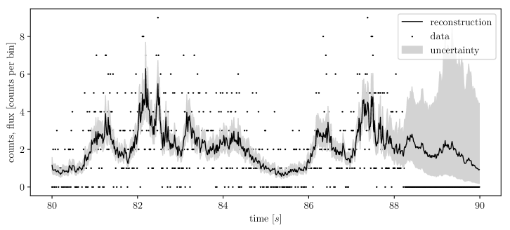
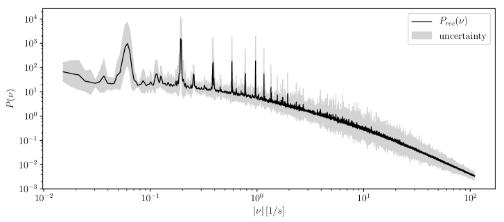
As for SGR1806-20, we were able to recover the frequency corresponding to the rotation as $\nu_{0}=0.1938\,$Hz, which is consistent with the reported $\nu_{0}=0.1923\,$Hz (Olausen & Kaspi 2014). For SGR 1900+14, the corresponding spectrum with the same smoothness prior $\sigma_{\mathrm{sm}}=5\times 10^{5}$ is more noisy because of the various operational down times of the instrument, which are marked grey in Figure 6(a). In Figure 6(b), we show a snapshot of the entire reconstructed light curve for a more detailed view. Even though no data were recorded between $88.245\,\text{s}\leq\text{t}\leq 95.1375\,\text{s,}$ the algorithm was able to infer a light curve by extrapolating from the data-constrained regions. This extrapolation is mainly driven by periodic features appearing in the data. As a further natural consequence, the one-$\sigma$ confidence interval increases drastically during down times. In total, these multiple operational down times of the instrument lead to fewer observed photons and in consequence to a weaker constrained reconstruction of the light curve as well as its power spectrum. Since a smoothness-enforcing prior $\sigma_{\mathrm{sm}}=5\times 10^{5}$ does not sufficiently denoise the light curve, we used a slightly stronger prior, $\sigma_{\mathrm{sm}}=10^{5}$ (Figure 7(a)), for our further analysis.

Table 3: All frequencies with $\chi_{0}>11$ and their multiplicity $n$ of the rotation period $\nu_{0}=0.1938$ [Hz] for SGR 1900+14.

$\nu$ [Hz]	$\chi_{0}$	$n$ [$\nu_{0}$]	$\nu$ [Hz]	$\chi_{0}$	$n$ [$\nu_{0}$]
7.693	13.214	39.7	11.768	13.718	60.7

With the same detection threshold as before, $\chi_{0}>11$, we find two candidate frequencies at $7.693\,$ and $11.768\,$Hz, see Table 3.

Table 4: Maximum $\chi_{0}$ at $\nu_{\text{max}}$ in a $5\%$ interval around previously observed oscillation frequencies $\nu$ for SGR 1900+14. We also list the local variance $\sigma_{\chi}$ of $\chi_{0}$ at this interval.

$\nu$ [Hz]	$\nu_{\text{max}}\,$[Hz] in $\pm 5\%$ interval	$\chi_{0,\text{max}}$	$\sigma_{\chi}$
28.0	27.341	5.392	2.931
53.5	54.781	5.24	2.318
84	86.328	4.39	2.228
155.1	161.719	3.777	1.582

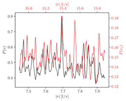
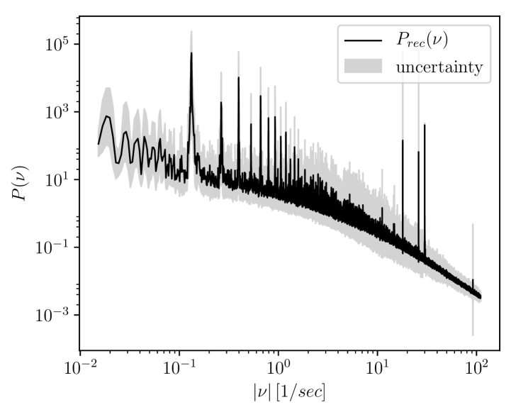
In Table 4 we give the maximum $\chi_{0}$ around previously observed frequencies. As for SGR 1806-20, we cannot confirm any of the previously detected frequencies, the highest significance we see is $\chi_{0}>5.4$ for $28.0\,$ Hz. We further investigated our combined criterium, but now reduced to the giant flare of SGR 1900+14 compared to the flare of SGR 1806-20. Figure 10 shows only one additional frequency at $\nu=7.695\,$Hz, which strengthens our confidence in the previous finding in Table 3 at $\nu=7.693\,$Hz. In Figure 8 we overplot the reconstructed power spectra around $\nu=7.693\,$Hz (black line) and its first overtone (red line). These two peaks are the largest in the given frequency range.

Figure 8: Zoomed-in view of the reconstructed power spectra of the giant flare SGR 1900+14 around $\nu\sim 7.693\,$Hz in black and its first overtone around $\nu\sim 15.386\,$Hz in red. The plot corresponds to $\sigma_{\mathrm{sm}}=1\times 10^{5}$ as in fig. 7(a).

Figure 9: Pulse profiles of different rotation periods overplotted for SGR 1900+14. The temporal evolution of the pulse profile is visible from blue to green to red. Smooth curves without significant short time-variability are reconstructed during instrument deadtimes.

Figure 10: Same as in Figure 5 for the SGR 1900+14 event, with $\sigma=10^{5}$. We indicate for all counts with $\chi_{0}\geq 5$ and $\chi_{1}\geq 5$ the corresponding frequency in Hertz and its multiple of the neutron star frequency $\nu_{0}=0.1938\,$Hz.

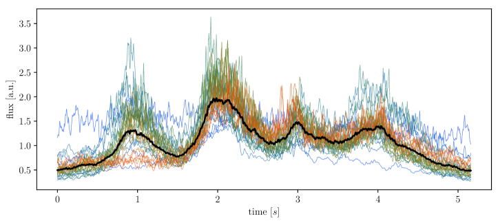
We plot the time evolution of the different pulses of SGR 1900+14 in Figure 9. As before, blue indicates the beginning of the flare, green the middle, and red the end. Here, the data are of inferior quality compared to the SGR 1806-20 and the parts of the curves without significant short time-variability are purely reconstructed by our algorithm. For SGR 1900+14 we observed four maxima, which also evolved differently compared to each other. For example, the weakest maximum ($\mathrm{time}\sim 1\,$s) declines almost monotonically with time, while the others remain rather constant with far less variability in time.

In order to facilitate secondary studies based on our reconstructions and spectra, we provide these data online at http://cdsweb.u-strasbg.fr/cgi-bin/qcat?J/A+A/. At www.mpa-garching.mpg.de/ift/data/QPO we also provides interactive plots of Figures 7, 1 and 3 for more detailed views.

4 Discussion

We recovered the rotation period of the two magnetars $\nu^{1806}=0.1323\,$ Hz and $\nu^{1900}=0.1938\,$Hz, and up to the $31$th overtone for SGR 1806-20 ($\chi_{0}>11$) and to the $18$th for SGR 1900+14 ($\chi_{0}>7.5$). In addition, we only found potential periodic signals at $9.2\,$Hz (SGR1806-20) and $7.7\,$Hz (SGR1900+14), which are significant in $\chi_{0}$ and in the combination of $\chi_{0}$ and $\chi_{1}$ according to our respective criterium. For SGR 1900+14 and with the single criterium on $\chi_{0}$, we found another candidate frequency at $\nu=11.8\,$Hz, with a similar $\chi_{0}$ as the signal at $7.7\,Hz,$ but without detected overtones. Therefore we only consider $\nu=7.7\,$Hz as a potential signal. The most robust feature is at $9.2\,$Hz for SGR 1806-20, it has the highest $\chi_{0}$ , and we detect some of its overtones as local maxima in $\chi_{0}$ at $18.3$ and $36.4\,$Hz, respectively. The two latter frequencies are similar to previously reported frequencies at $17.9$ (Watts & Strohmayer 2006) and $36.8\,$Hz (Hambaryan et al. 2011).

Although the reimplemented Bayesian inference algorithm D³PO proved (see Appendices A, B and C) its basic ability to reconstruct QPO in photon bursts in many tests, even in the low S/N regime, we cannot confirm the previously reported frequencies at $17,21,26,29,59,92.5,116,$ and $150\,$Hz for SGR 1806-20 and $28,53,84,$ and $155\,$Hz for SGR 1900+14. In particular, we show in Appendix C that our algorithm is able to recover sufficiently strong quasi-periodic signals around $90\,$Hz with a width of $\sim 0.6\,$Hz.

Our analysis and therefore all reconstructed power spectra and reconstructed photon fluxes depend on the particular chosen smoothness-enforcing prior $\sigma_{\mathrm{sm}}$ . Selecting a smaller $\sigma_{\mathrm{sm}}$ allows the algorithm to denoise the power spectrum even at low S/N. However, at high frequencies, the small $\sigma_{\mathrm{sm}}$ leads to a lower sensitivity for spectral lines. Therefore, a trade-off needs to be found for $\sigma_{\mathrm{sm}}$ between better denoising (small $\sigma_{\mathrm{sm}}$) and better sensitivity (large $\sigma_{\mathrm{sm}}$). Owing to the sharply deteriorating S/N for frequency ranges around $625\,$Hz and $1840\,$Hz, which would require a very small $\sigma_{\mathrm{sm}}$, we are currently not able to investigate these frequencies for QPOs.

We assume that our findings hold and determine the effect that the results have on the interpretation of the theoretical model of magnetar oscillations. First of all, the new candidate frequencies at $9.2\,$ and $7.7\,$Hz for SGR1806-20 and SGR1900+14, respectively, are much lower than the frequencies reported so far. Here, our method has a clear advantage over previous studies, as we can analyse the entire data set at once, meaning that no parts of the data set are left out. In principle, this leads to a more robust reconstruction and also counteracts statistical artefacts that may be introduced by a windowed analysis. Our method is fully noise-aware and has in principle no problems with observational dead times. If these two frequencies are related to neutron star oscillations, the parameters of current models change significantly. When we assume that the oscillations are pure crustal shear modes, the identification of the low frequency with the $n=0,l=2$ mode would favour models with rather low shear speeds and therefore EoS with a fast increase of symmetry energy (Steiner & Watts 2009). However, pure shear models are not very likely because of the strong interaction with the magnetic field in the interior of the star (Levin 2006, 2007; Gabler et al. 2011, 2012). If the magnetic field is not neglected, coupled magneto-elastic oscillations need to be considered. In this case, the much lower fundamental oscillation frequency indicates a magnetic field of the order of $\bar{B}\sim 6\times 10^{13}-3\times 10^{14}\,$G, lower by a factor of $\sim 3$ than our estimates in Gabler et al. (2013). With such weak magnetic fields, the oscillations would also remain confined to the core for models with very strong shear modulus, and there would be no chance to observe the oscillations exterior to the star. Therefore, similarly to the case of pure crustal shear oscillations, the low frequencies of $9.2\,$ or $7.7\,$Hz favour EoSs that give a small shear modulus. However, the estimation of the magnetic field strength has some serious problems : i) The spin-down estimate is only accurate to a factor of a few. ii) The particular magnetic field configuration inside a magnetar is unknown, meaning that even for dipolar-like fields in the exterior, there are different possible realization in the interior. iii) In addition to the degeneracies of the dipolar magnetic field strength and the magnetic field configuration, which lead to comparable frequencies, the compactness of the neutron star and the superfluid properties of the core matter also influence the frequencies significantly (Gabler et al. 2017). In order to advance and to lift some of these degeneracies, we need more observations of QPOs, and if possible, observations for different sources.

In respect of the potential of improving our method by modelling the spectra as an independent combination of a continuum and lines, we postpone a more thorough discussion of these consequences to future work. We also plan to improve our algorithm by taking the deadtime after each photon detection into account and include further instrument responses. However, we expect these improvements to increase our detection limits only by about a few per cent.

We have furthermore shown the capability of our code D³PO to denoise and recover the shape of the light curve. This may have interesting applications in the field of modelling the pulses of X-ray bursters.

5 Conclusion

We have applied a new Bayesian method, D³PO to analyse time-series data of the giant flares of SGR 1806-20 and SGR 1900+14. Thereby, we ensured that the photon shot noise, operational down times of the instrument, and the a priori unknown power spectrum of the photon flux were taken into account. In order to denoise and reconstruct the logarithmic photon flux and its power spectrum simultaneously from the data, we had to assume some kind of spectral smoothness on the power spectrum to counteract data variance. Our analysis cannot confirm previous findings of QPOs in the giant flare data, but we found new candidates for periodic signals at $9.2\,$Hz for SGR 1806-20 and $7.7\,$Hz for SGR1900+14. If these are real and related to the lowest frequency oscillation of the magnetar, our results favour high-compactness, weaker magnetic fields than were assumed before, and low shear moduli. The necessary application of a smoothness-enforcing prior results in a reduced sensitivity to the spectral line in the power spectrum. Hence, we propose for future work to decompose the power spectrum into two components, one smooth background spectrum, and one consisting of spectral lines. In this way, the previously reported lines may be confirmed or refuted with higher confidence, or additional and as yet unknown frequencies in QPOs might be discovered.

Appendix A Influence of the smoothness-enforcing parameter $\sigma$

To demonstrate the performance of the Bayesian inference algorithm, we challenged the new implementation of the algorithm with mock data. To do so, we drew Poisson samples from $\lambda=\@vec{R}e^{\@vec{s}}$. For simplicity, we assumed $\@vec{R}$ to be the identity operator. The signal field $\@vec{s}$ was drawn from a Gaussian random field $\@vec{s}\hookleftarrow\mathscr{G}(s,S)$, with

$$S_{\nu\nu^{\prime}}=\frac{27}{\left(1+\nu/\nu_{0}\right)^{2}}\delta_{\nu\nu^{\prime}}\,,$$ (4)

with $\nu_{0}=1$ absorbing the physical units. To test whether the algorithm can reconstruct discrete frequencies as well, we further injected four $\delta$-peaks into $S_{\nu\nu^{\prime}}$ at randomly chosen positions. The peak heights decrease at higher frequencies to be as realistic as possible. For the test we used a one-dimensional regular grid with with $2^{16}$ pixels, each with a volume of $1/1000$ seconds.
In Figure 11 we tested the principle capabilities of the algorithm under the above-mentioned setting while varying the strength of the smoothness enforcing parameter $\sigma_{\mathrm{sm}}$. In the scenario of $\sigma_{\mathrm{sm}}=10^{4}$, shown in Figures 11(a) and 11(b), the algorithm was able to recover the signal as well as the power spectrum well within the one-$\sigma$ confidence interval. However, the two highest injected frequencies could not be recovered, as their injected strength and therefore their effect on the data was too weak to be distinguished from the Poisson shot noise.
In comparison to Figure 11(b), Figure 11(c) shows the reconstructed power spectrum using a significantly weaker smoothness enforcing $\sigma_{\mathrm{sm}}=10^{5}$. As a first obvious consequence, the local variance of the spectrum increases by multiple orders of magnitude. However, the same two frequencies as with the stronger $\sigma_{\mathrm{sm}}$ were clearly recovered. As a further consequence of the smaller $\sigma_{\mathrm{sm}}$ , the power spectrum does not fully recover the shape of $S_{\nu\nu^{\prime}}$ as it picks up more noise features from the recovered map and data. For a detailed discussion and mathematical derivation of this smoothness-enforcing parameter, we refer to Oppermann et al. (2013).

(a)

(b)

(c)

Figure 11: Reconstruction, i.e. map and power spectra from mock data, created according to Appendix A. For clarity, Figure 11(a) only shows a snapshot of the events between $32.8\,\text{sec}\lesssim t\lesssim 33\,\text{sec}$. In addition to the raw photon counts, the black line shows the original signal $\@vec{s}$, as well as the reconstruction in red, including its uncertainty. Figure 11(b) shows the reconstructed power spectra as well as its uncertainty, as in Figure 11(a), using a smoothness-enforcing prior with $\sigma_{\mathrm{sm}}=10^{4}$. Figure 11(c) shows a reconstructed power spectrum with a weaker smoothness-enforcing prior with $\sigma_{\mathrm{sm}}=10^{5}$.

Appendix B Recovery of spectral lines at high frequencies

Now we estimate how strong periodic oscillations must be in order to be detectable in the reconstructed power spectrum. To be as close as possible to a realistic scenario, we manipulated the reconstructed photon flux of event SGR 1806-20. We added a periodic signal with discrete frequencies at $18.0,26.0,30.0,$ and $90.0$ Hz to the reconstructed $\@vec{\phi}$ shown in Figure 1(a). The relative strength of this additional photon flux was varied, between $10^{2}$ and $10^{5}$ times stronger than the local power of the injected frequencies. From these manipulated fluxes, we again drew Poisson samples and let the algorithm recover the power spectrum and the flux.
Figure 12 shows the reconstructed power spectra. In the setting of the top panel, we were only able to recover the injected frequency at $18$ Hz, the other three could not be inferred as their strength of $10^{2}$ compared to the local power was too weak to be identified as part of the signal and not the Poisson shot noise. However, as the one-$\sigma$ confidence interval of the reconstructed spectrum at $18\,\text{Hz}\lesssim\nu\lesssim 40\,\text{Hz}$ increases, the algorithm is just at the S/N threshold at which it is able to reconstruct discrete frequencies. If the injected strength of the frequencies, that is, the amplitude of the injected signal, becomes larger, as in Figure 12(b), the algorithm can infer all frequencies.
Hence, we may conclude that if the data show periodic signals at high frequencies with sufficient strength, they can be reconstructed by the algorithm. The strength of the periodic signal must therefore be at least $10^{2}$ times stronger than the local power of the signal in order to give a significant imprint on the reconstructed power spectrum.

(a)

(b)

Figure 12: Reconstructed power spectrum, according to the test scenario described in Appendix B. The strengths of the injected frequencies are $10^{2}$ (top) and $10^{5}$ (bottom) times stronger than the local power at these frequencies. The displayed uncertainties indicate the one-$\sigma$ confidence interval.

Appendix C Recovery of quasi-periodic oscillations

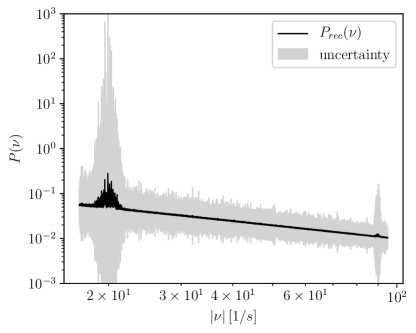
Here, we estimate how strong QPOs have to be for our algorithm to still find a significant signal in the reconstructed power spectrum. Similar to Appendix B, we used the reconstructed photon flux, Figure 1(a) of event SGR 1806-20, and added a quasi-periodic signal at around $20$ Hz and $90$ Hz. We assumed that the power spectrum of a QPO has an approximately Gaussian shape with variance $\sigma\approx 0.6$. From this manipulated flux, we drew Poisson samples and let the algorithm recover the power spectrum and the flux.

Figure 13: Smoothed Leahy power of the injected pure QPO-like signal. The two QPOs at $20$ Hz and $90$ Hz were reconstructed by D³PO, Figure 14.

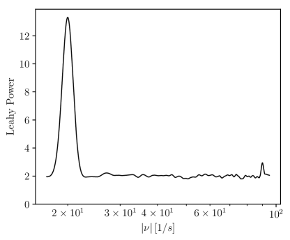
Figure 13 shows the power spectrum of the Poissonian photon counts for a pure QPO-like injected signal, smoothed with a Gaussian convolution kernel whose variance is the same as that of the injected QPO. The reconstructed power spectrum is shown in Figure 14. The S/N around $20$ Hz is much higher than the S/N around $90$ Hz. Therefore, the QPO at $20$ Hz has a significantly larger amplitude in the reconstructed power spectrum than that around $90$ Hz. The strength of the injected QPO at $90$ Hz is just at the threshold to give a significant signal in the reconstructed power spectrum. Thus, we may conclude that at this frequency, a QPO has to have a Leahy power of the order of $3$ in order be detectable by D³PO.

Figure 14: Reconstructed power spectrum according to the QPO injection test described in Appendix C. The displayed uncertainties indicate the one-$\sigma$ confidence interval.

References

- Cerdá-Durán et al. (2009) Cerdá-Durán, P., Stergioulas, N., & Font, J. A. 2009, MNRAS, 397, 1607
- Colaiuda et al. (2009) Colaiuda, A., Beyer, H., & Kokkotas, K. D. 2009, MNRAS, 396, 1441
- Colaiuda & Kokkotas (2011) Colaiuda, A. & Kokkotas, K. D. 2011, MNRAS, 414, 3014
- Deibel et al. (2014) Deibel, A. T., Steiner, A. W., & Brown, E. F. 2014, Phys. Rev. C, 90, 025802
- Duncan (1998) Duncan, R. C. 1998, ApJ, 498, L45
- Enßlin & Frommert (2011) Enßlin, T. A. & Frommert, M. 2011, Phys. Rev. D, 83, 105014
- Enßlin & Knollmüller (2016) Enßlin, T. A. & Knollmüller, J. 2016, ArXiv e-prints [arXiv:1612.08406]
- Gabler et al. (2011) Gabler, M., Cerdá Durán, P., Font, J. A., Müller, E., & Stergioulas, N. 2011, MNRAS, 410, L37
- Gabler et al. (2012) Gabler, M., Cerdá-Durán, P., Stergioulas, N., Font, J. A., & Müller, E. 2012, MNRAS, 421, 2054
- Gabler et al. (2013) Gabler, M., Cerdá-Durán, P., Stergioulas, N., Font, J. A., & Müller, E. 2013, Physical Review Letters, 111, 211102
- Gabler et al. (2016) Gabler, M., Cerdá-Durán, P., Stergioulas, N., Font, J. A., & Müller, E. 2016, MNRAS, 460, 4242
- Gabler et al. (2017) Gabler, M., Cerdá-Durán, P., Stergioulas, N., Font, J. A., & Müller, E. 2017, in preparation
- Glampedakis et al. (2011) Glampedakis, K., Andersson, N., & Samuelsson, L. 2011, MNRAS, 410, 805
- Glampedakis et al. (2006) Glampedakis, K., Samuelsson, L., & Andersson, N. 2006, MNRAS, 371, L74
- Hambaryan et al. (2011) Hambaryan, V., Neuhäuser, R., & Kokkotas, K. D. 2011, A&A, 528, A45+
- Huppenkothen et al. (2014a) Huppenkothen, D., D’Angelo, C., Watts, A. L., et al. 2014a, ApJ, 787, 128
- Huppenkothen et al. (2014b) Huppenkothen, D., Heil, L. M., Watts, A. L., & Göğüş, E. 2014b, ApJ, 795, 114
- Huppenkothen et al. (2014c) Huppenkothen, D., Watts, A. L., & Levin, Y. 2014c, ApJ, 793, 129
- Israel et al. (2005) Israel, G. L., Belloni, T., Stella, L., et al. 2005, ApJ, 628, L53
- Junklewitz et al. (2016) Junklewitz, H., Bell, M. R., Selig, M., & Enßlin, T. A. 2016, A&A, 586, A76
- Levin (2006) Levin, Y. 2006, MNRAS, 368, L35
- Levin (2007) Levin, Y. 2007, MNRAS, 377, 159
- Messios et al. (2001) Messios, N., Papadopoulos, D. B., & Stergioulas, N. 2001, MNRAS, 328, 1161
- Olausen & Kaspi (2014) Olausen, S. A. & Kaspi, V. M. 2014, ApJS, 212, 6
- Oppermann et al. (2013) Oppermann, N., Selig, M., Bell, M. R., & Enßlin, T. A. 2013, Phys. Rev. E, 87, 032136
- Passamonti & Lander (2013) Passamonti, A. & Lander, S. K. 2013, MNRAS, 429, 767
- Passamonti & Lander (2014) Passamonti, A. & Lander, S. K. 2014, MNRAS, 438, 156
- Piro (2005) Piro, A. L. 2005, ApJ, 634, L153
- Pumpe et al. (2016) Pumpe, D., Greiner, M., Müller, E., & Enßlin, T. A. 2016, Phys. Rev. E, 94, 012132
- Samuelsson & Andersson (2007) Samuelsson, L. & Andersson, N. 2007, MNRAS, 374, 256
- Samuelsson & Andersson (2009) Samuelsson, L. & Andersson, N. 2009, Classical and Quantum Gravity, 26, 155016
- Selig & Enßlin (2015) Selig, M. & Enßlin, T. 2015, A&A, 574, A74
- Selig et al. (2015) Selig, M., Vacca, V., Oppermann, N., & Enßlin, T. A. 2015, A&A, 581, A126
- Sotani et al. (2016) Sotani, H., Iida, K., & Oyamatsu, K. 2016, New A, 43, 80
- Sotani et al. (2007) Sotani, H., Kokkotas, K. D., & Stergioulas, N. 2007, MNRAS, 375, 261
- Sotani et al. (2008) Sotani, H., Kokkotas, K. D., & Stergioulas, N. 2008, MNRAS, 385, L5
- Sotani et al. (2013) Sotani, H., Nakazato, K., Iida, K., & Oyamatsu, K. 2013, MNRAS, 428, L21
- Steiner & Watts (2009) Steiner, A. W. & Watts, A. L. 2009, Physical Review Letters, 103, 181101
- Steininger et al. (2017) Steininger, T., Dixit, J., Frank, P., et al. 2017, ArXiv e-prints [arXiv:1708.01073]
- Strohmayer & Watts (2005) Strohmayer, T. E. & Watts, A. L. 2005, ApJ, 632, L111
- Strohmayer & Watts (2006) Strohmayer, T. E. & Watts, A. L. 2006, ApJ, 653, 593
- Thompson & Duncan (1995) Thompson, C. & Duncan, R. C. 1995, MNRAS, 275, 255
- van Hoven & Levin (2011) van Hoven, M. & Levin, Y. 2011, MNRAS, 410, 1036
- van Hoven & Levin (2012) van Hoven, M. & Levin, Y. 2012, MNRAS, 420, 3035
- Watts & Strohmayer (2006) Watts, A. L. & Strohmayer, T. E. 2006, ApJ, 637, L117