Abstract

The persistent homology pipeline includes the reduction of a, so-called, boundary matrix. We extend the work of bauer2014clear ; chen2011persistent where they show how to use dependencies in the boundary matrix to adapt the reduction algorithm presented in edelsbrunner2002topological in such a way as to reduce its computational cost. Herein we present a number of additional dependencies in the boundary matrices and propose a novel parallel algorithm for the reduction of boundary matrices. In particular, we show: that part of the reduction is immediately apparent, give bounds on the reduction needed for remaining columns, and from these give a framework for which the boundary reduction process can be massively parallelised. Simulations on four synthetic examples show that the computational burden can be conducted in approximately a thousandth the number of iterations needed by traditional methods. Moreover, whereas the traditional boundary reductions reveal barcodes sequentially from a filtration order, this approach gives an alternative method by which barcodes are partly revealed for multiple scales simultaneously and further refined as the algorithm progresses; simulations show that for a Vietoris-Rips filtration with $\sim 10^{4}$ simplices, an estimate of the essential simplices with 95% precision can be computed in two iterations and that the reduction completed to within 1% in about ten iterations of our algorithm as opposed to nearly approximately eight thousand iterations for traditional methods.

1 Introduction

Persistent homology is a technique within topological data analysis, see edelsbrunner2002topological ; ghrist2014elementary and references therein, that estimates the topological features of a shape in high-dimensional space from a point-cloud $S\subset\mathbb{R}^{d}$ sampled from a data manifold $\mathcal{M}\subset\mathbb{R}^{d}$. The topological information on the shape $\mathcal{M}$ is encoded as a set of Betti numbers,

$$\operatorname{Betti}(\mathcal{M}):=\{b_{p,r}:0\leq p\leq d,r\in[0,\infty)\}$$ (1)

which geometrically represent the number of $p$-dimensional holes at scale $r\in[0,\infty)$ in a simplicial complex triangulation of $\mathcal{M}$. Knowledge of the homologies persistent in a dataset can aid interpretation of the data, see for example carlsson2009topology ; carlsson2014topological ; carlsson2008local ; chan2013topology ; lum2013extracting ; taylor2015topological ; nicolau2011topology . In the persistent homology paradigm, the set $\operatorname{Betti}(\mathcal{M})$ is approximated at multiple scales $\{r_{1},\dots,r_{T}\}\subset[0,\infty)$ through a two-step procedure. First, a scale-indexed filtration of simplicial complexes is constructed yielding a simplicial complex $K$ with vertex set $S$ and $m$ simplices. This simplicial complex is represented as a $m\times m$ matrix $\partial$ defined over the Galois field of two elements $\mathbb{F}_{2}$ and having $\partial_{i,j}=1$ iff $\sigma_{i}\in K$ is a face of $\sigma_{j}\in K$ with co-dimension $1$. The matrix $\partial\in\mathbb{F}_{2}^{m\times m}$, together with the scale $r_{\ell}$ at which each simplex $\sigma_{j}\in K$ is added to the filtration, encode the necessary information to estimate $\operatorname{Betti}(\mathcal{M})$ via persistent homology. The homologies in the data are then revealed in the second, and final, step of reducing the boundary matrix $\partial$. Reduction algorithms for persistent homology are so named as they can essentially be viewed as acting on each column of the boundary matrix to minimise the maximum index of its nonzeros while maintaining that the column span of the first $j$ columns of $\partial$ remains unchanged for all $j$. That is, following the notation of chen2011persistent , reduction algorithms entrywise minimise

$$\operatorname{low_{\partial}}(j)=\left\{\begin{array}[]{ll}\max\{i\in[m]:\partial_{i,j}=1\}&\mbox{if $\partial_{j}\neq 0$}\\ 0&\mbox{if $\partial_{j}=0$,}\end{array}\right.$$ (2)

subject to the aforementioned span constraint; we denote the minimum of $\operatorname{low_{\partial}}(j)$ by $\operatorname{low^{*}}(j)$. Nonzero values of $\operatorname{low^{*}}(j)$ reveal a homology persisting from $\sigma_{\operatorname{low^{*}}(j)}$ to $\sigma_{j}$. As $\operatorname{low^{*}}(j)$ is a property of the simplicial complex $K$ edelsbrunner2010computational we omit the explicit reference to the boundary matrix in its notation; moreover, we denote by $\operatorname{low_{\partial}}$ and $\operatorname{low^{*}}$ the vectors of their values in $\{0,1,\dots,m\}.$ Sec. 2.1 and 2.2 provides further details on the construction of the simplicial complex filtration, the persistent homology pipeline, and their connections with the underlying data manifold as they pertain to our main results.

The focus of this manuscript is extending the work bauer2014clear ; chen2011persistent where they show how to use dependencies in the boundary matrix to adapt the first boundary matrix reduction algorithm edelsbrunner2002topological , restated in Alg. 1, in such a way as to reduce its computational cost.

Data: $\partial\in\mathbb{F}_{2}^{m\times m}$

Result: $\operatorname{low^{*}}\in\mathbb{Z}_{m+1}^{m}$

for $j\in[m]$ do

       while $\exists$ $j_{0}<j$ : $\operatorname{low_{\partial}}(j_{0})=\operatorname{low_{\partial}}(j)$ do

             $\partial_{j}\leftarrow\partial_{j}+\partial_{j_{0}}$;

            

       end while

      

end for

$\operatorname{low^{*}}\leftarrow\operatorname{low_{\partial}}$;

Algorithm 1 Standard reduction edelsbrunner2002topological

Alg. 1 performs the reduction by sequentially minimising $\operatorname{low_{\partial}}(j)$ by adding columns $j_{0}<j$ for which $\operatorname{low_{\partial}}(j_{0})=\operatorname{low_{\partial}}(j)$ until either there is no such column $j_{0}$ or column $j$ has been set to zero. The computational overhead in Alg. 1 is in computing the left-to-right column operations, and has a worst-case complexity of $\mathcal{O}(m^{3})$ which is achieved by an example simplicial complex in morozov2005persistence . Previous advances in reduction algorithms primarily focus on decreasing the computational cost by exploiting structure in $\partial$ to reveal some entries in $\partial$ can be set to zero bauer2014clear ; chen2011persistent or by parallelising the reduction by dividing the boundary matrix into blocks and partially reducing each block bauer2014clear ; bauer2014distributed ; further details of these approaches are given in Sec. 2.4. The aforementioned approaches show substantially improved average empirical operation count as compared to Alg. 1.

Our main contribution is by noting both bounds on the values of $\operatorname{low^{*}}(j)$, which are empirically observed to typically identify a large fraction of the $\operatorname{low^{*}}(j)$, and moreover presenting a framework by which the known $\operatorname{low^{*}}(j)$ can be used to to reduce $\partial$ in a highly parallel fashion. In addition, the bounds on $\operatorname{low^{*}}(j)$ suggest priorities by which columns might be reduced. The algorithm is designed to work with some of the previous speedups as suggested in bauer2014clear . Moreover, as is discussed in Sec. 3, our parallelisation strategy induces an iterative non-local refinement procedure on $\operatorname{low_{\partial}}$ and makes the algorithm fit for early stopping, see Secs. 4.2 and 4.3. An example of the a resulting reduction algorithm is given in Alg. 2 whose details are explained further in Sec. 3 and numerical experiments for its application are shown in Sec. 4. Additional strategies to speed up the algorithm are given in Secs. 3.2 and 3.3, while Sec. 3.4 suggests further extensions for computer environments with substantially fewer processors than $m$.

Data: $\partial\in\mathbb{F}_{2}^{m\times m}$; $\operatorname{\mbox{MAX\_ITER}}\in[m]$

Result: $\operatorname{low^{*}}\in\mathbb{Z}_{m+1}^{m}$

// Phase 0: Initialisation

Build $\beta_{j}$ according to (9);

$\operatorname{\mathsf{Pivots}}\leftarrow\left\{j\in[m]:\beta_{j}=\operatorname{low_{\partial}}(j)>0\right\}$;

for $j\in\operatorname{\mathsf{Pivots}}$ do

       $\partial_{\operatorname{low_{\partial}}(j)}\leftarrow 0$;

      

end for

$\operatorname{iter}\leftarrow 0$;

while $\operatorname{low_{\partial}}\neq\operatorname{low^{*}}$ or $\operatorname{iter}\leq\operatorname{\mbox{MAX\_ITER}}$ do

       // Phase I: Local injections

       for $d\in[\dim(K)]$ do

             $\operatorname{maxCollision}\leftarrow 0$;

             for $j\in\left\{\ell\in K_{d}:\operatorname{low_{\partial}}(\ell)>0\right\}\setminus\operatorname{\mathsf{Pivots}}$ do

                   if $\operatorname{low_{\partial}}(j)>\operatorname{maxCollision}$ then

                         if $\operatorname{low_{\partial}}(j)\notin\operatorname{low_{\partial}}([j-1])$ then

                               $\operatorname{\mathsf{Pivots}}\leftarrow\operatorname{\mathsf{Pivots}}\cup\left\{j\right\}$;

                              

                        else

                               $\operatorname{maxCollision}\leftarrow\operatorname{low_{\partial}}(j)$;

                              

                         end if

                        

                   end if

                  

             end for

            

       end for

      // Phase II: Column reduction

       for $j_{0}\in\operatorname{\mathsf{Pivots}}$ do

             $\mathcal{N}(j_{0})\leftarrow\left\{\ell\in[m]\setminus[j_{0}]:\operatorname{low_{\partial}}(\ell)=\operatorname{low_{\partial}}(j_{0})\right\}$;

             for $j\in\mathcal{N}(j_{0})$ do

                   $\partial_{j}\leftarrow\partial_{j}+\partial_{j_{0}}$;

                   if $\operatorname{low_{\partial}}(j)=\beta_{j}$ then

                         $\operatorname{\mathsf{Pivots}}\leftarrow\operatorname{\mathsf{Pivots}}\cup\left\{j\right\}$;

                         $\partial_{\operatorname{low_{\partial}}(j)}\leftarrow 0$;

                        

                   end if

                  

             end for

            

       end for

      // Increase iteration

       $\operatorname{iter}\leftarrow\operatorname{iter}+1$;

      

end while

$\operatorname{low^{*}}\leftarrow\operatorname{low_{\partial}}$;

Algorithm 2 Parallel multi-scale reduction

2 Background

In this section we give an overview of the pipeline for computing persistent homology which includes a short introduction to the topological and algebraic results on which our results are based, and a review of the prior art in boundary matrix reduction algorithms. In what follows we adopt the following notation. If $S$ is a set, we let $2^{S}$ denote the power set of $S$ and $|S|$ be the cardinality of $S$. We also borrow notation from Combinatorics and let $[m]:=\{1,\dots,m\}$ for $m\in\mathbb{N}$. We will use $\mathbb{Z}_{m+1}$ as a shorthand for $[m]\cup\{0\}$. For a function $f:A\rightarrow B$, we let $f(A)=\left\{f(a)\in B:a\in A\right\}$ and $f(\emptyset)=\emptyset$. If $\partial\in\mathbb{F}_{2}^{m\times m}$ is a matrix, we let $\partial_{j}\in\mathbb{F}_{2}^{m}$ be its $j$-th column and $\partial_{i,\cdot}$ be its $i$-th row. The support of an $m$-dimensional vector $v$ is defined as $\operatorname{supp}(v)=\left\{i\in[m]:v_{i}\neq 0\right\}$. If $\partial\in\mathbb{F}_{2}^{m\times m}$ is a boundary matrix, we let $\operatorname{nnz}(\partial)$ or the number of nonzeros entries in $\partial$. We reserve the notation $\operatorname{\mathds{1}}\left\{\cdot\right\}$ for indicator functions that return $1$ if the argument is true and $0$ otherwise. If $\mathbb{R}^{d}$ is the $d$-dimensional Euclidean space with $p$-norm $\|\cdot\|_{p}$ and $S\subset\mathbb{R}^{d}$, we let $\operatorname{diam}(S):=\max_{x,y\in S}\|x-y\|$ be the diameter of $S$. Finally, for any $c\in\mathbb{R}^{d}$ and $r\geq 0$, we let $\operatorname{\mathcal{B}}_{r}(c):=\left\{x\in\mathbb{R}^{d}:\|x-c\|_{p}\leq r\right\}$ be the $d$-dimensional $p$-ball of radius $r$ centred at $c$.

2.1 Simplicial homology

If $S$ is a finite set and $\alpha\subset\sigma\subset S$, then $\sigma$ is a simplex of $S$ and $\alpha$ is a face of $\sigma$. A set of simplices $K\subset 2^{S}$ is a simplicial complex if $\sigma\in K$ implies that every face of $\sigma$ is also in $K$. The dimension of the simplex is defined as $\dim(\sigma)=|\sigma|-1$. The dimension of a simplicial complex $K$ will be defined as $\dim(K)=\max\left\{\dim(\sigma):\sigma\in K\right\}$. It will be convenient to assume that the simplices in $K$ are indexed, so that $K=\left\{\sigma_{1},\dots,\sigma_{|K|}\right\}$. In this case, the set of $p$-simplices is the set of simplices in $K$ which are indexed by

$$K_{p}=\left\{j\in[|K|]:\dim(\sigma_{j})=p\right\}.$$ (3)

The boundary of a simplex $\sigma$ is its set of faces of co-dimension one; symbolically we denote this by $\operatorname{bd}(\sigma)=\{\alpha:\dim(\alpha)=\dim(\sigma)-1\}$.

In the subsequent paragraphs we describe, for completeness, the algebraic structure of simplicial complexes and how it gives rise to the homology groups; omitting this paragraph does not limit one’s ability to understand the new algorithms proposed. The set of $p$-chains $\mathsf{C}_{p}(K):=2^{K_{p}}$ equipped with the symmetric difference operation is an abelian group with neutral element $\emptyset$. For each $p\in\mathbb{N}$, the group $\mathsf{C}_{p}(K)$ is related to $\mathsf{C}_{p-1}(K)$ by a boundary map $d_{p}:\mathsf{C}_{p}\rightarrow\mathsf{C}_{p-1}$ defined by $d_{p}(c)=\sum_{\sigma\in c}\operatorname{bd}(\sigma)$. The kernel and image of $d_{p}$ are geometrically meaningful. Elements in $\mathsf{Z}_{p}=\operatorname{Ker}d_{p}$ are called $p$-cycles, while elements in $\mathsf{B}_{p}=\operatorname{Im}d_{p+1}$ are called $p$-boundaries. Moreover, for all $p$ and for all $c\in\mathsf{C}_{p}$, $d_{p-1}\circ d_{p}(c)=\emptyset$, so $\mathsf{B}_{p}\subset\mathsf{Z}_{p}\subset\mathsf{C}_{p}$, see edelsbrunner2010computational . The quotient space $\mathsf{H}_{p}={\mathsf{Z}_{p}}/{\mathsf{B}_{p}}$ is called the $p$-th homology group and its elements are called homology classes. The $p$-th Betti number is defined as $b_{p}=\operatorname{rank}\mathsf{H}_{p}$ and counts the number of $p$-dimensional holes of the simplicial complex $K$.

2.2 Construction of the simplicial complex

In persistent homology, a simplicial complex $K$ is built from a point-cloud $S\subset\mathbb{R}^{d}$ sampled from a data manifold $\mathcal{M}\subset\mathbb{R}^{d}$. Given $S$, the goal of persistent homology is to estimate the relevant homological features of $\mathcal{M}$ at all scales $r\in[0,\infty)$. To do so, a simplicial complex triangulation is computed from $S$ at all scales $r\in\{r_{1},\dots,r_{T}\}\subset[0,\infty)$ by letting $K=\emptyset$ and adding a simplex $\sigma\subset S$ to $K$ whenever the points in $\sigma$ are sufficiently close to each other. The notion of closeness is implied by the relevant scale parameter, and is assessed for each scale $r$ via a monotonic function $f_{r}:2^{S}\rightarrow\{0,1\}$ inducing a filtration

$$\mathbf{M}_{0}\subset\mathbf{M}_{1}\subset\cdots\subset\mathbf{M}_{T}=K$$ (4)

of simplicial complexes $\mathbf{M}_{i}=\left\{\sigma\in 2^{S}:f_{r_{i}}(\sigma)=1\right\}$. For example, the function

$$f_{r}(\sigma)=\operatorname{\mathds{1}}{\left\{\bigcap_{x_{0}\in\sigma}\operatorname{\mathcal{B}}_{r}(x_{0})\right\}},$$

generates the C̆ech complex filtration, while the function

$$f_{r}(\sigma)=\operatorname{\mathds{1}}\left\{\operatorname{diam}(\sigma)\leq 2r\right\}$$

generates the Vietoris-Rips complex filtration. We shall assume that the filtration (4) has $m$ elements and that the largest set in the filtration is a simplicial complex with simplices given by

$$K=\left\{\sigma_{1},\dots,\sigma_{m}\right\}.$$

It is further assumed that the simplices in $K$ are indexed according to a compatible ordering, meaning that the simplices in $\mathbf{M}_{\ell}$ always precede the ones in $K\setminus\mathbf{M}_{\ell}$, and that the faces of any given simplex always precede the simplex.

Persistent homology tracks how the homology of the filtration changes at each scale $r_{t}$ or, equivalently, as new simplices are added to the filtration. Indeed, when adding simplex $\sigma_{i}$ at scale $r_{t}$, the homology of $\mathbf{M}_{t}$ can change in one of two possible ways edelsbrunner2010computational .

1. A class of dimension $\dim(\sigma_{i})$ is created. In this case, $\sigma_{i}$ is a positive simplex.

2. A class of dimension $\dim(\sigma_{i})-1$ is destroyed. In this case, $\sigma_{i}$ is a negative simplex.

If $\sigma_{j}$ is a negative simplex, then it destroys the class created by a positive simplex $\sigma_{i}$ with $i=\operatorname{low^{*}}(j)<j$, see Lemma 1. This observation induces a natural pairing $(\sigma_{i},\sigma_{j})$ between a negative simplex $\sigma_{j}$ and the positive simplex $\sigma_{i}$ it destroys. Moreover, it allows us to quantify the lifetime of a particular homology class in the filtration via its homology persistence which is the difference between $r_{t}$ for $\sigma_{j}$ and $\sigma_{i}$.

When $r_{T}$ is sufficiently small, we might find that some simplices are never destroyed; these simplices represent the homology classes that are persistent in the filtration up to scale $r_{T}$, and we called them essential. The persistence pairs are computed by representing the filtration (4) as a boundary matrix $\partial\in\mathbb{F}_{2}^{m\times m}$ and applying the reduction algorithm edelsbrunner2002topological to it. We discuss this process in Sec. 2.3

2.3 Boundary matrix reduction

If $K=\{\sigma_{1},\dots,\sigma_{m}\}$ is a simplicial complex constructed as in the previous Sec. 2.2, it can be represented with a boundary matrix $\partial\in\mathbb{F}_{2}^{m\times m}$ defined by

$$\partial_{i,j}=\left\{\begin{array}[]{ll}1&\mbox{$\sigma_{i}$ is a face of $\sigma_{j}$ of co-dimension 1}\\ 0&\mbox{otherwise}\end{array}\right.$$ (5)

The boundary matrix $\partial$ is sparse, binary, and upper-triangular and has associated a function $\operatorname{low_{\partial}}:[m]\rightarrow\mathbb{Z}_{m+1}$ defined as in (2). The matrix $\partial$ will be said to be reduced when $\operatorname{low_{\partial}}\in\mathbb{Z}_{m+1}^{m}$ is an injection over its support, $i.e.$ when $\operatorname{low_{\partial}}(j_{1})=\operatorname{low_{\partial}}(j_{2})>0$ implies that $j_{1}=j_{2}$. We use the notation $\partial^{*}$ to denote a matrix $\partial$ with injective $\operatorname{low_{\partial}}$ and remark that even though $\partial$ can have several reductions, the injection is a property of the complex $K$ and does not depend on any particular reduction $\partial^{*}$, see (edelsbrunner2010computational, , p.183). When there is no risk of confusion, we let $\operatorname{low^{*}}$ be the injection of the boundary matrix under consideration.

The vector $\operatorname{low^{*}}$ reveals information about the pairings by virtue of the following Lemma.

Lemma 1 (Pairing edelsbrunner2002topological ).

If $\sigma_{j}$ is a negative simplex, then $\sigma_{\operatorname{low^{*}}(j)}$ is a positive simplex.

Hence, $\operatorname{low^{*}}(\cdot)$ partitions the simplices in $K$ as,

$$\operatorname{\mathsf{Pos}} =\{j\in[m]:\operatorname{low^{*}}(j)=0\}$$

$$\operatorname{\mathsf{Neg}} =\{j\in[m]:\operatorname{low^{*}}(j)>0\}$$

$$\operatorname{\mathsf{Ess}} =\{j\in\operatorname{\mathsf{Pos}}:\nexists\;k\;\operatorname{\mbox{s.t.}}\;\operatorname{low^{*}}(k)=j\}$$

so $\operatorname{\mathsf{Pos}}\cap\operatorname{\mathsf{Neg}}=\emptyset$ and $\operatorname{\mathsf{Ess}}\subset\operatorname{\mathsf{Pos}}$. It will also be convenient to define the set $\operatorname{\mathsf{Paired}}$ as the union of the set of negative and associated positive simplices

$$\operatorname{\mathsf{Paired}}=\left\{j\in[m]:\operatorname{low^{*}}(j)\in[m]\right\}\cup\left\{\operatorname{low^{*}}(j)\in[m]:j\in[m]\right\}$$ (6)

The technology used to reduce $\partial$ is known as the reduction algorithm (Alg. 1) and was first presented in edelsbrunner2002topological . The convergence guarantees of Alg. 1 are given in Theorem 2.

Theorem 2 (Convergence of Alg. 1 edelsbrunner2002topological ).

Alg. 1 converges for any boundary matrix $\partial\in\mathbb{F}_{2}^{m\times m}$ in at most $\mathcal{O}(m^{3})$ operations.

We survey the prior art in boundary matrix reduction algorithms in the subsequent Sec. 2.4.

2.4 Boundary matrix algorithm prior art

Let $K$ be the simplicial complex corresponding to a filtration over a grid $\{r_{1},\dots,r_{T}\}$ and point-cloud $S\subset\mathbb{R}^{d}$. The number of simplices in $K$ is of order $\Omega(2^{|S|})$ as $r_{T}\rightarrow\operatorname{diam}(S)$, which turns the process unfeasible even for moderately large point-clouds $S$ and scales $r_{T}$. Hence, though Alg. 1 terminates in $\mathcal{O}(m^{3})$ steps, we may find that $m=\mathcal{O}(2^{|S|})$ making the reduction unfeasible. The main computational overhead when reducing a boundary matrix is in performing left-to-right column operations, so many reduction algorithms have implemented strategies that cut the number of column operations required to fully reduce the matrix. One such strategy was given in chen2011persistent ; bauer2014clear by reducing columns in blocks of decreasing dimension and observing that, by Lemma 1, column $\operatorname{low^{*}}(j)$ can be set to zero whenever column $j$ is reduced. As $\dim(\sigma_{\operatorname{low^{*}}(j)})$ is of one lower dimension that $\dim(\sigma_{j})$, clearing results in all positive non-essential columns of dimension less than $\dim(K)$ being set to zero without zeroing them through column additions. Setting a positive column to zero when its corresponding negative pair has been found is often called clearing, so we adopt this terminology. Alg. 2 heavily relies on this clearing strategy so we sketch the pseudocode of chen2011persistent in Alg. 3.

Data: $\partial\in\mathbb{F}_{2}^{m\times m}$

Result: $\operatorname{low^{*}}\in\mathbb{Z}_{m}^{m+1}$

for $d\in\{\dim K,\dim K-1,\dots,1\}$ do

       for $j\in K_{d}$ do

             while $\exists j_{0}<j:\operatorname{low_{\partial}}(j_{0})=\operatorname{low_{\partial}}(j)$ do

                   $\partial_{j}\leftarrow\partial_{j}+\partial_{j_{0}}$;

                  

             end while

            if $\partial_{j}\neq 0$ then

                   $\partial_{\operatorname{low_{\partial}}(j)}\leftarrow 0$;

                  

             end if

            

       end for

      

end for

$\operatorname{low^{*}}\leftarrow\operatorname{low_{\partial}}$;

Algorithm 3 Standard reduction with a twist chen2011persistent

Another strategy to reduce the complexity of Alg. 1 is called compression (bauer2014clear, ) and consists in deriving analytical guarantees to nullify nonzeros in the boundary matrix without affecting the pairing of the simplices. This has the objective of saving arithmetic operations and hence reducing the flop count. However for very large values of $m$, which are typical for large filtration values where $m$ grows exponentially with $|S|$, it is necessary to also parallelise these approaches in order to be scalable. The idea of distributing the workload of the reduction algorithm has already been explored in (bauer2014clear, ; bauer2014distributed, ) where the matrix is partitioned into $b$ blocks of contiguous columns to be independently reduced in a shared-memory or distributed system. The numerical simulations in bauer2014distributed show that these strategies can indeed bring substantial speed-ups when implemented on a cluster, but also requires the provision of the parameter $b$ as well as a number of design choices for a practical implementation.

Apart from parallelisation, a number of other approaches have been proposed. For instance, milosavljevic2011zigzag adapted the Coppersmith-Winograd algorithm coppersmith1990matrix to guarantee reduction in time $\mathcal{O}(m^{2.3755})$. A set of sequential algorithms that exploits duality of vector spaces was given in de2011dualities ; de2011persistent , but as pointed out in otter2015roadmap is only known to give speed-ups when applied to Vietoris-Rips complexes. Finally, sheehy2014persistent projects $\partial$ to a low-dimensional space while controlling the error between the resulting barcodes, but doing so in practice can be as costly as reducing the matrix in its ambient space.

3 Main contributions

In this section we describe the theory behind the parallelisation strategy of Alg. 2. The main algorithmic innovation is a strategy to efficiently distribute the workload of Alg. 1 over $\mathcal{O}(m)$ processors to progressively entrywise minimize $\operatorname{low_{\partial}}\in\mathbb{Z}_{m+1}^{m}$. Additionally, Alg. 2 is designed to take advantage of some structural patterns in the boundary matrix in order to minimise the total number of left-to-right column operations. The core observation is that, by simple inspection, the rows of the boundary matrix reveal a subset of nonzero entries in $\partial$ which cannot be modified in the reduction process, and consequently identify nonzero lower bounds on $\operatorname{low^{*}}(j)$ for a subset of $j\in[m]$. This observation is captured by Definition 3 and Definition 4.

Definition 3 ($\operatorname{left}(\cdot)$).

Let $\partial\in\mathbb{F}_{2}^{m\times m}$ be a boundary matrix. The $\operatorname{left}$ function is defined as

$$\operatorname{left}(i)=\left\{\begin{array}[]{ll}\min\left\{j\in[m]:\partial_{i,j}=1\right\}&\partial_{i,\cdot}\neq 0\\ 0&\partial_{i,\cdot}=0\end{array}\right.$$ (7)

Definition 4 ($\beta_{j}$).

Let $\partial\in\mathbb{F}_{2}^{m\times m}$ be a boundary matrix and

$$\mathcal{L}_{j}=\{i\in[m]:\operatorname{left}(i)=j\}.$$ (8)

Then, for $j\in[m]$ we let

$$\beta_{j}=\left\{\begin{array}[]{ll}\max\mathcal{L}_{j}&\mathcal{L}_{j}\neq\emptyset\\ 0&\mathcal{L}_{j}=\emptyset\end{array}\right.$$ (9)

The vector $\beta\in\mathbb{Z}_{m+1}^{m}$ carries a great deal of information about the nature of each column in the boundary matrix. Some of its properties are explored in Theorem 5.

Theorem 5 (Properties of $\beta_{j}$).

Let $\partial\in\mathbb{F}_{2}^{m\times m}$ be a boundary matrix and $\beta$ defined as in (9). Then, the following statements hold.

1. $\beta_{j}=0\Leftrightarrow\nexists i\in[m]\operatorname{\mbox{s.t.}}\operatorname{left}(i)=j$

2. $\beta_{j}$ is invariant to left-to-right column operations.

3. $\{j\in[m]:\beta_{j}>0\}\subset\operatorname{\mathsf{Neg}}$.

4. $\operatorname{\mathsf{Pos}}\subset\{j\in[m]:\beta_{j}=0\}$.

5. $\beta_{j}\leq\operatorname{low^{*}}(j)\leq\operatorname{low_{\partial}}(j)$ for all $j\in[m]$.

6. $\beta$ can be computed in time $\mathcal{O}(\operatorname{nnz}(\partial))$.

Proof.

 

1. This follows directly from the definition of $\beta_{j}$.

2. Let $i\in[m]$ be a row of $\partial$ and $j=\operatorname{left}(i)$. Reduction of $\partial_{j}$ is achieved by adding to $\partial_{j}$ columns $\partial_{\ell}$ for $\ell<j$ By Definition 8 $\partial_{i,\ell}=0$ for $\ell<j$ and hence $\partial_{i,j}=1$ throughout the reduction. Consequently the set $\operatorname{left}(i)$ and values $\beta_{j}$ are fixed in the reduction procedure.

3. If $\beta_{j}>0$, then exists $i\in[m]$ such that $\operatorname{left}(i)=j>0$. Then, $\partial_{i,j}=1$ and there does not exist $\partial_{\ell}$ with $\ell<j$ such that $\partial_{i,\ell}=1$. Hence $\partial_{i,j}$ can not be set to zero in the reduction, so $j\in\operatorname{\mathsf{Neg}}$.

4. This result follows by taking complements on the result P.3.

5. By P.2 the set $\mathcal{L}_{j}$ in 8 are nonzero entries in $\partial_{j}$ which cannot be modified in the reduction procedure and consequently $\operatorname{low^{*}}(j)\geq\beta_{j}$.

   $$\operatorname{low^{*}}(j)\geq\max\{i\in\operatorname{supp}(\partial_{j}):\operatorname{left}(i)=j\}=\beta_{j}$$

6. Note that when creating the boundary matrix, $\beta$ can be constructed with the following procedure,

   Data: Simplicial complex $K=\left\{\sigma_{1},\dots,\sigma_{m}\right\}$

   Result: $\beta_{j}$ for $j\in[m]$

   for $\sigma_{j}\in K$ do

          $\beta_{j}\leftarrow 0$;

          for $\sigma_{i}\in\operatorname{bd}(\sigma_{j})$ do

                if $\sigma_{i}$ has not been visited then

                      $\beta_{j}\leftarrow\max(\beta_{j},i)$;

                      Mark $\sigma_{i}$ as visited;

                     

                end if

               

          end for

         

   end for

   Algorithm 4 Building $\beta$

   Alg. 4 finishes in time proportional to $\sum_{j}|\operatorname{bd}(\sigma_{j})|$, so it has complexity $\mathcal{O}\left(\operatorname{nnz}(\partial)\right)$.

∎

The value of Theorem 5 is most immediately apparent in P.4 and in particular when $\operatorname{low_{\partial}}(j)=\beta_{j}$ in which case $\operatorname{low^{*}}(j)$ is determined. Our numerical experiments in Sec. 4 show empirically that a large number of columns can usually be identified as already being reduced without need of any column operations. Moreover, having access to a large number of reduced columns allows a massive parallelisation as described in Sec. 3.1 and illustrated in Sec. 4. While the calculation of $\beta$ adds an initial computation to Alg. 2, it can be computed at the matrix-reading cost of $\mathcal{O}(\operatorname{nnz}(\partial))$, so it can often be obtained as a by-product of creating the filtration without penalising the asymptotic computational complexity of constructing the matrix.

Additionally, the vector $\beta$ gives a sufficient condition for a column to be in $\operatorname{\mathsf{Neg}}$. Knowledge that an unreduced column is necessarily negative can be used in numerous ways. For example, as discussed in sections 3.2, 3.3, and 3.4 this is useful to produce more reliable estimations of $\operatorname{low^{*}}$ in the case of early-stopping. Additionally, knowledge that a column is necessarily negative enhances a notion of clearing as discussed in Sec. 3.2.

Apart from Theorem 5, Alg. 2 makes use of the observation that since $\operatorname{low_{\partial}}$ converges to an injection $\operatorname{low^{*}}$, one can often inspect the sparsity pattern of $\partial$ to identify regions of $[m]$ where $\operatorname{low_{\partial}}$ is locally an injection. This local injection property is the basis of the following Theorems 6 and 7, which give sufficient conditions to identify sets $T\subset[m]$ such that $\operatorname{low_{\partial}}(j)=\operatorname{low^{*}}(j)$ for all $j\in T$. In the remainder of this section it will be convenient to extend some of our prior notation as follows: for a set $T\subset[m]$, we let $\operatorname{low_{\partial}}(T)=\left\{\operatorname{low_{\partial}}(j):j\in T\right\}$ and $|\operatorname{low_{\partial}}(T)|$ be its cardinality. Informally, the argument in Theorem 6 is that, for each dimension $d$, any subset of contiguous columns $T\subset K_{d}\setminus\{j\in K_{d}:\operatorname{low_{\partial}}(j)=0\}$ with $\min T=\min K_{d}$ is already reduced if $\operatorname{low_{\partial}}:T\rightarrow[m]$ is an injection or, equivalently, if $|\operatorname{low_{\partial}}(T)|=|T|$.

Theorem 6 (Local injection I).

Let $\partial\in\mathbb{F}_{2}^{m\times m}$ be the boundary matrix of a simplicial complex $K$ and let $d\in[\dim(K)]$ and $K_{d}$ defined as in (3). Let

$$T:=K_{d}\setminus\left\{j\in K_{d}:\operatorname{low_{\partial}}(j)=0\right\}\neq\emptyset$$

be such that $T=\left\{j_{1},\dots,j_{|T|}\right\}$ for $j_{1}<\cdots<j_{|T|}$ and for $\ell\leq|T|$, let $T^{\ell}=\left\{j_{1},\dots,j_{\ell}\right\}$. If

$$\left|\operatorname{low_{\partial}}\left(T^{\ell}\right)\right|=\ell,$$ (10)

then $\operatorname{low_{\partial}}(j)=\operatorname{low^{*}}(j)$ for all $j\in T^{\ell}$.

Proof.

Let $T$ be defined as in Theorem 6. If $\ell=1$, then there $\partial_{j_{1}}$ is the first column of dimension $d$ that appears in the filtration, so there is no column $j\in[j_{1}]$ that can reduce it. Hence, suppose that $\ell>1$ and let $j_{t}\in T^{\ell}$ be such that $\operatorname{low_{\partial}}(j_{t})\neq\operatorname{low^{*}}(j_{t})$. Then there is $j<j_{t}$ such that $\operatorname{low_{\partial}}(j)=\operatorname{low_{\partial}}(j_{t})$. This implies that $j\in K_{d}\cap[j_{t}]$ and that $\operatorname{low_{\partial}}(j)>0$, so $j\in T_{\ell}$. Hence, $|T_{\ell}|=\ell$, but $|\operatorname{low_{\partial}}(T_{\ell})|<\ell$, which contradicts (10). ∎

Theorem 7 addresses a generalisation of Theorem 6 and argues that for each dimension $d$, any subset of contiguous columns $T\subset K_{d}\setminus\{j\in K_{d}:\operatorname{low_{\partial}}(j)=0\}$ is already reduced if $|\operatorname{low_{\partial}}(T)|=|T|$ and there is no column $j\in K_{d}\setminus T$ with $j<\min T$ such that $\operatorname{low_{\partial}}(j)\in\operatorname{low_{\partial}}(T)$.

Theorem 7 (Local injection II).

Let $\partial\in\mathbb{F}_{2}^{m\times m}$ be the boundary matrix of a simplicial complex $K$ and let $d\in[\dim(K)]$. Define $T$ and $T^{\ell}$ as in Theorem 6. Assume that for $k>1$ and $k\leq\ell$ it holds that

$$\min\operatorname{low_{\partial}}(T^{\ell}\setminus T^{k-1})>\max\operatorname{low_{\partial}}(T^{k-1})$$ (11)

and

$$\left|\operatorname{low_{\partial}}\left(\left\{j_{k},\dots,j_{\ell}\right\}\right)\right|=\ell-k+1.$$ (12)

Then, $\operatorname{low_{\partial}}(j)=\operatorname{low^{*}}(j)$ for all $j\in\left\{j_{k},\dots,j_{\ell}\right\}$.

Proof.

Let $T$ and $T^{\ell}$ be as in Theorem 7 so that $T^{\ell}\setminus T^{k-1}=\left\{j_{k},\dots,j_{\ell}\right\}$. Since $\ell>0$ and $k>1$, then $\ell-k+1>0$. If $k=2$, then $j_{2}\in\operatorname{low_{\partial}}(T^{\ell}\setminus T^{1})$ and invoking (11),

$$\operatorname{low_{\partial}}(j_{2})\geq\min\operatorname{low_{\partial}}(T^{\ell}\setminus T^{1})>\max\operatorname{low_{\partial}}(T^{1})=\operatorname{low_{\partial}}(j_{1}),$$

so the result follows by invoking Theorem 6 with $\ell=2$. Arguing as in Theorem 6, suppose that $k>2$ and let $j_{t}\in\left\{j_{k},\dots,j_{\ell}\right\}$ be such that $\operatorname{low_{\partial}}(j_{t})\neq\operatorname{low^{*}}(j_{t})$. Then, there is $j<j_{t}$ such that $\operatorname{low_{\partial}}(j)=\operatorname{low_{\partial}}(j_{t})$. Given that $j_{k}\leq j<j_{t}$ and by (11) then $j\in T^{\ell}\setminus T^{k-1}$. Hence, $|\operatorname{low_{\partial}}(T_{\ell}\setminus T^{k-1})|<\ell-k+1$, which contradicts (12). ∎

We now describe how the results presented so far in this section interact in Alg. 2.

3.1 Parallel multi-scale reduction

So far, Theorems 5 -7 identify a subset of the columns $j$ in $\partial\in\mathbb{F}_{2}^{m\times m}$ for which $\operatorname{low^{*}}(j)$ is known without need for performing column additions. In order to complete the reduction of $\partial$, that is identify $\operatorname{low^{*}}$, it is necessary to perform column additions analogous to those in Alg. 1; however,unlike the sequential ordering in Alg. 1, we will propose massive parallelisation of the column additions. Towards this we define the set of columns $j\in[m]$ for which their $\operatorname{low^{*}}(j)$ is known at any given iteration of a reduction algorithm as the Pivots:

$$\operatorname{\mathsf{Pivots}}=\left\{j\in[m]:\operatorname{low^{*}}(j)\in[m]\mbox{ has been identified. }\right\}$$

Moreover, we define the set of column with which a pivot could be added to in order to reduce their $\operatorname{low_{\partial}}$ as the neighbours of column $j$:

$$\operatorname{\mathcal{N}}(j)=\left\{\ell>j:\operatorname{low_{\partial}}(\ell)=\operatorname{low^{*}}(j)\right\}.$$ (13)

Note that as $\operatorname{low^{*}}$ are an injection, if $j_{1},j_{2}\in\operatorname{\mathsf{Pivots}}$ and $j_{1}\neq j_{2}$, then $\mathcal{N}(j_{1})\cap\mathcal{N}(j_{2})=\emptyset$ so

$$\left(\bigcup_{j\in\operatorname{\mathsf{Pivots}}}\operatorname{\mathcal{N}}(j)\right)\bigcup\operatorname{\mathsf{Pivots}}\subset[m]$$ (14)

is a partition and each column in $\mathcal{N}(j)$ for $j\in\operatorname{\mathsf{Pivots}}$ can have their low reduced independently by adding column $j$ to columns $\ell\in\operatorname{\mathcal{N}}(j)$. In sequential algorithms like Algs. 1 and 3, the set $\mathcal{N}(j)$ is constructed only after the block $[j-1]\cap K_{\dim(\sigma_{j})}$ has been fully reduced. In contrast, Alg. 2 starts by inspecting the sparsity pattern of $\partial$ to identify a large set of seed $\operatorname{\mathsf{Pivots}}$ that are then used to build (13) for each $j\in\operatorname{\mathsf{Pivots}}$. Given that (14) is a partition, each set $\mathcal{N}(j)$ is partially reduced independently, typically in parallel and new columns are appended to $\operatorname{\mathsf{Pivots}}$ whenever their update is such that their $\operatorname{low^{*}}(\ell)$ is identified by either by Theorems 5 - 7. We elaborate on these stages of Alg. 2, and its convergence, in the remainder of this section.

3.1.1 Phase 0: Initialising $\operatorname{\mathsf{Pivots}}$

The first step of Alg. 2 is to compute the vector $\beta$, which can be done at cost $\mathcal{O}(\operatorname{nnz}(\partial))$ by Theorem 5. This vector is then coupled with $\operatorname{low_{\partial}}$ to build the set of initial pivots

$$\operatorname{\mathsf{Pivots}}\leftarrow\left\{j\in[m]:\beta_{j}=\operatorname{low_{\partial}}(j)\right\},$$

which by Theorem 5, contains indices for columns that are already reduced, e.g. $\operatorname{low^{*}}(j)$ is known for $j\in\operatorname{\mathsf{Pivots}}$. The clearing strategy from Lemma 1 is applied to each of these columns to zero out their corresponding positive pairs. The resulting set of $\operatorname{\mathsf{Pivots}}$ is then passed on to the main iteration.

3.1.2 Phase I: Finding local injections

In the first phase of the main iteration, the following Alg. 5 is applied to each dimension $d\in[\dim(K)]$.

Data: $\partial\in\mathbb{F}_{2}^{m\times m}$; $\operatorname{\mathsf{Pivots}}\subset\operatorname{\mathsf{Neg}}$

Result: $\operatorname{\mathsf{Pivots}}^{\prime}\subset\operatorname{\mathsf{Neg}}$ $\operatorname{\mbox{s.t.}}$ $\operatorname{\mathsf{Pivots}}\subset\operatorname{\mathsf{Pivots}}^{\prime}$

$\operatorname{maxCollision}\leftarrow 0$;

for $j\in\left\{\ell\in K_{d}:\operatorname{low_{\partial}}(\ell)>0\right\}\setminus\operatorname{\mathsf{Pivots}}$ do

       if $\operatorname{low_{\partial}}(j)>\operatorname{maxCollision}$ then

             if $\operatorname{low_{\partial}}(j)\notin\operatorname{low_{\partial}}([j-1])$ then

                   $\operatorname{\mathsf{Pivots}}\leftarrow\operatorname{\mathsf{Pivots}}\cup\left\{j\right\}$;

                  

            else

                   $\operatorname{maxCollision}\leftarrow\operatorname{low_{\partial}}(j)$;

                  

             end if

            

       end if

      

end for

Algorithm 5 Finding local injections

Alg. 5 starts by initialising $\operatorname{maxCollision}\leftarrow 0$ and walking through the non-zero columns in $K_{d}$ that have not been identified as pivots. The idea is to identify regions of $K_{d}$ where Theorems 6 and 7 can be applied to guarantee that a local injection exists. At each $j$, the variable $\operatorname{maxCollision}$ tracks the largest $i\in\operatorname{low_{\partial}}([j-1])\cap\operatorname{low_{\partial}}(K_{d})$ such that $i=\operatorname{low_{\partial}}(j_{1})=\operatorname{low_{\partial}}(j_{2})$ for $j_{1}\neq j_{2}$. In terms of Theorem 7, $\operatorname{maxCollision}$ plays the rôle of $\max\operatorname{low_{\partial}}(T^{j-1})$ in (11), since if $\operatorname{low_{\partial}}(j)>\operatorname{maxCollision}$ and $\operatorname{low_{\partial}}(j)\notin\operatorname{low_{\partial}}([j-1])$, then there is no column $\ell<j$ that can have $\operatorname{low_{\partial}}(\ell)=\operatorname{low_{\partial}}(j)$ and consequently $\operatorname{low_{\partial}}(j)$ cannot be further reduced and therefore its $\operatorname{low^{*}}(j)$ is known.

3.1.3 Main iteration II: Parallel column reduction

Once the first phase has been completed, the sets of $\operatorname{\mathcal{N}}(j)$ are computed for each $j\in\operatorname{\mathsf{Pivots}}$. Each column in $\bigcap_{j\in\operatorname{\mathsf{Pivots}}}\operatorname{\mathcal{N}}(j)$ has their associated pivot added to them; that is, $\partial_{\ell}\leftarrow\partial_{\ell}+\partial_{j}$ is carried out for each $\ell\in\mathcal{N}(j)$ for $j\in\operatorname{\mathsf{Pivots}}$. Alg. 2 then marks the column $\ell$ as reduced if $\operatorname{low_{\partial}}(\ell)=\beta_{\ell}$, $\\ ell$ is added to the set of $\operatorname{\mathsf{Pivots}}$, and the clearing strategy is called to set the associated positive column $\partial_{\operatorname{low^{*}}(\ell)}$ to zero.

3.1.4 Convergence

The convergence of Alg. 2 is a consequence of the interplay between Phases I and II of the main iteration. We describe this mechanism in the following theorem.

Theorem 8 (Convergence of Alg. 2).

Let $\partial\in\mathbb{F}_{2}^{m\times m}$ be the boundary matrix of a simplicial complex $K$. Then, Alg. 2 converges to $\operatorname{low^{*}}$.

Proof.

Let $\operatorname{\mathsf{Pivots}}^{\ell}\subset[m]$ be the set of indices of columns that are known to be already reduced at the start of iteration $\ell$, and let $\operatorname{low_{\partial}}^{\ell}$ be the corresponding estimate of $\operatorname{low^{*}}$. We show that Alg. 1 converges by showing that if $\operatorname{low^{*}}\neq\operatorname{low_{\partial}}^{\ell}$, then either

$$|\operatorname{\mathsf{Pivots}}^{\ell+1}|\geq|\operatorname{\mathsf{Pivots}}^{\ell}|+1$$ (15)

or,

$$\|\operatorname{low_{\partial}}^{\ell+1}-\operatorname{low^{*}}\|<\|\operatorname{low_{\partial}}^{\ell}-\operatorname{low^{*}}\|.$$ (16)

Note that $|\operatorname{\mathsf{Pivots}}^{0}|\geq\dim(K)\geq 1$ since at Phase 0 at least the first column of each dimension must be identified as a pivot.

Suppose that at the start of iteration $\ell\geq 0$ the boundary matrix $\partial$ is still not reduced so that $\operatorname{low_{\partial}}^{\ell}\neq\operatorname{low^{*}}$. If a column is identified as reduced at the end of Phase I, then it is marked as a pivot so $|\operatorname{\mathsf{Pivots}}^{\ell+1}|\geq|\operatorname{\mathsf{Pivots}}^{\ell}|+1$ and we are done. Hence, assume that no new pivots are identified. In this case, for each $j\in\operatorname{\mathsf{Pivots}}^{\ell}$ we construct the set $\mathcal{N}(j)$ as in (13).

If $\exists j_{0}\in\operatorname{\mathsf{Pivots}}^{\ell}$ such that $|\mathcal{N}(j_{0})|\geq 1$, then Alg. 2 enters Phase II to reduce columns in $\mathcal{N}(j_{0})$. In this case, (16) holds and we are done. Otherwise, suppose $|\mathcal{N}(j_{0})|=0$ for all $j\in\operatorname{\mathsf{Pivots}}^{\ell}$. In this case, since the matrix is not reduced, the set

$$\mathcal{C}=\left\{j\in[m]:\left|\mathcal{N}(j)\right|>0\right\}$$

is not empty. Let,

$$j_{\min}=\min\mathcal{C}$$ (17)

and let $d=\dim(\sigma_{j_{\min}})$. There are two possible cases,

1. $j_{\min}=\min K_{d}$: In this case, the column must have been identified as a pivot at Phase 0, which is a case previously excluded.

2. $j_{\min}>\min K_{d}$: Let

   $$T=K_{d}\setminus\left\{j\in K_{d}:\operatorname{low_{\partial}}(j)=0\right\}.$$

   In this case, it must hold that $|\operatorname{low_{\partial}}([j_{\min}]\cap T)|=|[j_{\min}]\cap T|$ since otherwise, there would exist an $\ell\in[j_{\min}-1]\cap T$ such that $\operatorname{low_{\partial}}(\ell)=\operatorname{low_{\partial}}(j_{\min})$ implying that $|\mathcal{N}(\ell)|>0$ and thus contradicting the minimality of $j_{\min}$. Hence, by Theorem 6, $\operatorname{low_{\partial}}([j_{\min}]\cap T)=|[j_{\min}]\cap T|$, so $j_{\min}$ must have been identified at Phase I of the iteration. This is again, a contradiction.

Therefore, it is impossible to have $|\mathcal{N}(j_{0})|=0$ for all $j_{0}\in\operatorname{\mathsf{Pivots}}^{\ell}$ if no pivots were identified at Phase I of the iteration. Hence, as long as $\operatorname{low_{\partial}}^{\ell}\neq\operatorname{low^{*}}$ either (15) or (16) hold, so at each iteration Alg. 2 will increase the number of pivots, decrease some entries in $\operatorname{low_{\partial}}$, or both. ∎

The multi-scale nature of Alg. 2 is advantageous to implement a number of strategies that allow us progressively refine our knowledge of $\operatorname{low^{*}}$. We describe some of these strategies in the next subsections.

3.2 Clearing by compression

In this section we describe a clearing strategy based on a column compression arguments inspired by the previous compression arguments presented in bauer2014clear to reduce operation flop-count. This strategy, in its simplest form presented in Corollary 10, can be straightforwardly implemented in a parallel architecture in Alg. 2, but is not explicitly listed in Alg. 2 for conciseness. Here, we present a compression result that can in some cases help clear columns in the matrix and in some other cases can give improved bounds on the location of $\operatorname{low^{*}}$. In doing so, it will be convenient to define the set $\operatorname{\mathsf{Paired}}^{\ell}\subset\operatorname{\mathsf{Paired}}$, as the sets of elements in (6) that have been identified at the $\ell$-th iteration by Alg. 2.

Note that $\operatorname{\mathsf{Paired}}^{\ell}$ at iteration $\ell$ include the set of unreduced columns that have been identified as negative. In particular, by Theorem 5,

$$\left\{j\in[m]:\beta_{j}>0\right\}\subset\operatorname{\mathsf{Paired}}^{\ell}.$$

Lemma 9 (Clearing by local compression).

Let $\partial\in\mathbb{F}_{2}^{m\times m}$ be a boundary matrix of a simplicial complex $K$. Let $j\in[m]$ and $d=\dim(\sigma_{j})\in[\dim(K)]$. Then at iteration $\ell$ of Alg. 2,

$$\operatorname{low^{*}}(j)\in L_{j}:=\left\{0\right\}\cup\left(K_{d-1}\cap[\beta_{j},\operatorname{low_{\partial}}(j)]\right)\setminus\operatorname{\mathsf{Paired}}^{\ell}.$$ (18)

Proof.

If $j\in[m]$, and $d=\dim(\sigma_{j})$, then $\operatorname{low^{*}}(j)\in K_{d-1}$ by the definition of $\partial$; moreover, $\operatorname{low^{*}}(j)\in[\beta_{j},\operatorname{low_{\partial}}(j)]$ by Theorem 5. The injection condition on the support of $\operatorname{low^{*}}$ implies that if $\operatorname{low^{*}}(j)$ can not be equal to any of the observed positive $\operatorname{low^{*}}$’s. Finally, $\operatorname{low^{*}}(j)$ can not be equal to the index of any of the identified negative columns as $\partial_{\operatorname{low^{*}}(j)}$ is necessarily positive, and can not be equal to any of the indices of paired positive columns by the injection condition and Lemma 1. Hence, $\operatorname{low^{*}}(j)\notin\operatorname{\mathsf{Paired}}^{\ell}$. ∎

Lemma 9 implies the following corollary,

Corollary 10.

Let $\partial\in\mathbb{F}_{2}^{m\times m}$ and let $L_{j}$ be defined as in (18) and such that $|L_{j}|=1$. Let $i\in L_{j}$. If $i=0$, then $\operatorname{low^{*}}(j)=0$. Else, $i=\operatorname{low^{*}}(j)$ and consequently column $j$ is negative and fully reduced and $\partial_{i}$ is positive.

3.3 Essential estimation

Another way to reuse the partial knowledge of negative and associated positive columns, as given by $\operatorname{\mathsf{Paired}}^{\ell}\subset\operatorname{\mathsf{Paired}}$ be the set of columns that have been identified as paired at the $\ell$-th iteration of Alg. 2, is to estimate the essential simplices

Lemma 11 (Essential estimation).

Let $\partial\in\mathbb{F}_{2}^{m\times m}$ be a boundary matrix and $j\in[m]$, then at iteration $\ell$

$$\operatorname{\mathsf{Ess}}\subset\left\{[m]\setminus\operatorname{\mathsf{Paired}}^{\ell}\right\}\setminus\left\{\operatorname{low_{\partial}}(j):j\in[m]\right\}$$ (19)

Proof.

Clearly, $\operatorname{\mathsf{Ess}}\cap\operatorname{\mathsf{Paired}}^{\ell}=\emptyset$ for all $\ell$ by the partition on the columns. We show that $\operatorname{\mathsf{Ess}}\cap\left\{\operatorname{low_{\partial}}(j):j\in[m]\right\}=\emptyset$. To do this, we follow a proof by contradiction and suppose that $\operatorname{low_{\partial}}(j)\in\operatorname{\mathsf{Ess}}$, which implies

$$\nexists p\operatorname{\mbox{s.t.}}\operatorname{low^{*}}(p)=\operatorname{low_{\partial}}(j)$$ (20)

as otherwise $p$ is the index of a negative column and $\operatorname{low^{*}}(p)$ the index of an associated positive non-essential column. We show that column $j$ can not be either positive or negative, which leads to a contradiction.

1. $j\in\operatorname{\mathsf{Pos}}$: As we are determining $\operatorname{\mathsf{Ess}}\cap\left\{\operatorname{low_{\partial}}(j):j\in[m]\right\}$, we consider only the $j$ such that $\operatorname{low_{\partial}}(j)>0$, but since $j\in\operatorname{\mathsf{Pos}}$ we must have $\operatorname{low^{*}}(j)=0$. By the definition of $j$ being positive there must exist $q<j$ such that $\operatorname{low^{*}}(q)=\operatorname{low_{\partial}}(j)$ in order that $j$ can be reduced to the zero column; however, this contradicts (20) by setting $p=q$.

2. $j\in\operatorname{\mathsf{Neg}}$: By Theorem 5 $\operatorname{low_{\partial}}(j)\geq\operatorname{low^{*}}(j)$. If $\operatorname{low_{\partial}}(j)=\operatorname{low^{*}}(j)$, then (20) is contradicted with $p=j$. Otherwise, if $\operatorname{low_{\partial}}(j)>\operatorname{low^{*}}(j)$, then by the definition of $\operatorname{low^{*}}(j)$ there must exist $q<j$ such that $\operatorname{low^{*}}(q)=\operatorname{low_{\partial}}(j)$ in order to reduce column $j$. This again, contradicts (20)

∎

Theorem 19 implies that the set of essential columns can be iteratively estimated by a set $E^{\ell}\subset[m]$ initialised at $E^{0}=[m]$ and iteratively updated as,

$$E^{\ell+1}\leftarrow\left(E^{\ell}\setminus\operatorname{\mathsf{Paired}}^{\ell}\right)\setminus\left\{\operatorname{low_{\partial}}(j):j\in[m]\right\}.$$ (21)

3.4 Distributing the workload

Central to the efficacy of Alg. 2 is the typically large number of pivots available to reduce subsequent columns coupled with the ability of all column additions in its Phase 2 to be performed in parallel. We do not explicitly describe parallelisation strategies for Phase 2 due to architecture specificity, but make a few remarks regarding communication minimisation and early termination in Secs. 3.4.1 and 3.4.2 respectively.

3.4.1 Prioritise reduction of sets $\mathcal{N}(j)$ with large cardinality

Let,

$$\mathcal{C}=\left\{j\in\operatorname{\mathsf{Pivots}}:|\mathcal{N}(j)|>0\right\},$$ (22)

be the set of columns that can be used in a given iteration to decrease $\operatorname{low_{\partial}}$.

If only $p<|\mathcal{C}|$ processors are available, and communication of these active pivots is the dominant cost, then it may be desirable to implement only a portion of the possible column additions available in Phase 2 duration an iteration. In such a setting, a priority queue can be used to order the sets $\mathcal{N}(j)$ based on their cardinality and act on multiples of $p$ sets of active columns per iteration of Phase 2.

3.4.2 Prioritise reduction of $\mathcal{N}(j)\cap\operatorname{\mathsf{Neg}}$

In settings where $\operatorname{low^{*}}$ cannot be fully determined due to computational or time constraints, the reduction ordering can be prioritised to minimize various objectives. One such objective is to minimize $\|\operatorname{low_{\partial}}-\operatorname{low^{*}}\|$ in a suitable norm as rapidly as possible. Recall, Theorem 5 gives bounds on the value of $\operatorname{low^{*}}$ and $\operatorname{low_{\partial}}$ is available by inspection. Due to the the identification of fully reduced negative column, say column $j$ allows clearing of column $\operatorname{low^{*}}(j)$ there is benefit in prioritising the reduction of columns which are known to be negative, e.g. $\left\{j\in[m]:\beta_{j}>0\right\}\subset\operatorname{\mathsf{Neg}}$. Alternative prioritisations would be application specific, but can include such information as prioritising values for which the persistence is greater or improving the estimation of essential columns as described in Sec. 3.3.

4 Numerical experiments

In this section we evaluate the efficacy of our parallel multi-scale reduction Alg. 2 empirically by comparing its performance against the standard reduction Alg. 1 and standard reduction with a twist Alg. 3. Our evaluation is on a set of synthetic simplicial complexes from point-clouds sampled from a set of a predefined set of ensembles. The point-clouds and their corresponding Rips-Vietoris simplicial complexes are generated with the Javaplex (Javaplex, ) library. When building the simplicial complex, we supply the following parameters,

1. Number of points ($N$): The number of points in the point-cloud to be generated.

2. Maximum dimension ($\dim K$): The maximum dimension of the resulting simplicial complex $K$.

3. Maximum filtration value ($r_{T}$): The maximum radius in a predefined grid of scales $\left\{r_{1},\dots,r_{T}\right\}\subset[0,\infty)$ used to build the filtration.

4. Number of divisions ($h$): The grid of scales is uniform with spacing $h$, that is $h:=r_{i+1}-r_{i}$ for $i\in[T-1]$.

$$\begin{array}[]{l | c c c c}\mbox{ Ensemble }&N&\dim K&r_{T}&h\\ \hline\cr\hline\cr\mbox{ Gaussian Points in $\mathbb{R}^{3}$}&15&5&5&10\\ \mbox{ Figure-8}&15&5&5&10\\ \mbox{ Trefoil Knot}&15&5&5&10\\ \mbox{ $\mathbb{S}^{2}\times\mathbb{S}^{2}$}&15&5&5&10\end{array}$$

Central to our numerical evaluations in this manuscript is the number of iterations required. The reduction in Algs. 1 and 3 is an horizontal procedure in the sense that no column in a given dimension is reduced before the preceeding columns in this dimension have been reduced. In contrast, Alg. 2 is a diagonal procedure as it implements an horizontal type of reduction in Phases I and II, but rather than completely reducing the columns in order, it progressively prunes the matrix vertically by doing left-to-right column operations every time there is enough information to guarantee that this is possible. Given this crucial difference in design, it becomes difficult to find appropriate benchmarking scenarios and, more fundamentally, to provide a notion of iteration that is agnostic to the algorithm’s architecture. Hence, in our numerical experiments, we let an iteration be the set of operations that are performed at each cycle of the outer-most loop of the algorithm. This is a reasonable convention as it is consistent with each of the algorithm’s concurrency and is also natural for the high-level pseudo-code description of their design. However, we note that this notion of iteration can be optimistic or pessimistic depending on the unit of computational overhead that is being measured. In our experiments, left-to-right column operations are chosen as the main unit of computational overhead and, indeed, our algorithm has been designed to minimise this kind of operations. Given the embarrassingly parallel nature of Phase II of Alg. 2, this model is generous with our algorithm as it does not consider possible limitations to the number of processors available and it does not account for the communication overhead between processors. Finally, as our algorithm’s practical performance is greatly limited by the hardware architecture, we point out that our numerical experiments should serve as a proof-of-concept of a design that can yield a powerful production implementation rather than a trustworthy comparison of the run-time or flop-count in the general case.

The numerical results presented in this section simulate a parallel implementation and are available at githubRepo . A truly parallel implementation is being developed.

4.1 Operations are packed in fewer iterations

For each ensemble we sample three point-clouds and reduce their corresponding boundary matrices using each of Algs. 1 - 3. Fig. 1 illustrates the computational complexity, as the number of column additions performed at each iteration and also the number of nontrivial xor operations when adding columns in the matrix; that is, the number of scalar operations of the form

$$\left\{1\oplus 1,1\oplus 0,0\oplus 1\right\}.$$

Scalar operations are relevant because in some storage models like the one given in chen2011persistent the computational cost of updating the matrix depends super-linearly on the number of non-zeros in the columns being added. Figs. 1a, 1g and 1j show the number of column additions per iteration of each algorithm performs to reduce each of the simplicial compelexes under consideration. Specifically, they illustrate how that Alg. 2 allocates most of the column additions at the earliest iterations due to its highly parallel nature. On the other hand, Figs. 1b, 1h, and 1k as well as Tab. 1 show that while Alg. 2 reduces the number of iterations, it has a total number of column additions indistingushable to Alg. 3 and about half that of Alg. 1. This shows that Alg. 2 is successful in packing the number of left-to-right column operations into considerably few independent iterations.

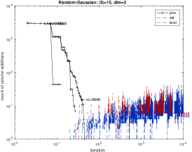
(a) Gaussian; Count of column additions

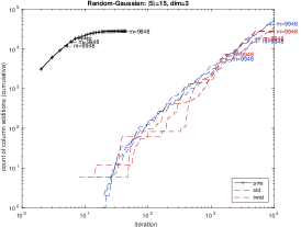
(b) Gaussian; Count of column additions (cumulative)

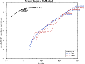
(c) Gaussian; Count of XOR operations (cumulative)

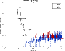
(d) Figure-8; Count of column additions

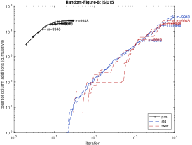
(e) Figure-8; Count of column additions (cumulative)

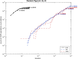
(f) Figure-8; Count of XOR operations (cumulative)

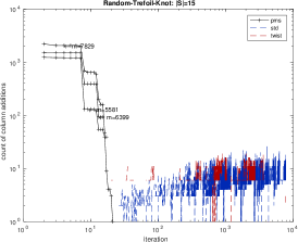
(g) Trefoil Knot; Count of column additions

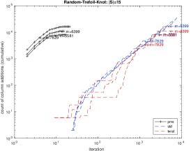
(h) Trefoil Knot; Count of column additions (cumulative)

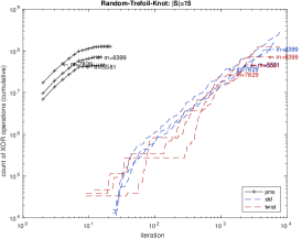
(i) Trefoil Knot; Count of XOR operations (cumulative)

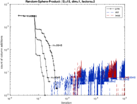
(j) Sphere product; Count of column additions

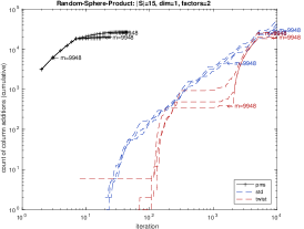
(k) Sphere product; Count of column additions (cumulative)

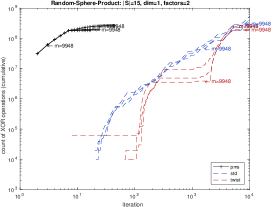
(l) Sphere product; Count of XOR operations (cumulative)

Figure 1: Benchmarking on column operation overhead. For each ensemble, three point clouds are sampled and their corresponding simplicial complexes are reduced with Algs. 1 - 3. Their performance is benchmarked in three different ways: through the number of column additions done at each iteration (Figs. 1a, 1d, 1g, 1j); through the cumulative number of column additions up to a given iteration (Figs.  1b, 1e, 1h, 1k); and through the cumulative number of XOR operations done up to a given iteration (Figs.  1c, 1f, 1i, 1l).

Sample	Gaussian		Figure-8		Trefoil-knot		Sphere-product
	std	twist	std	twist	std	twist	std	twist
1	0.52	1.00	0.49	1.00	0.46	1.00	0.50	1.00
2	0.52	1.00	0.51	1.00	0.40	1.00	0.49	1.01
3	0.50	1.00	0.50	1.00	0.44	1.00	0.47	1.00

Table 1: Ratio of total column additions. For each ensemble, three point clouds are sampled and the corresponding simplicial complexes are reduced with each algorithm. The ratio of total column additions between Alg. 2 and both Algs. 1 and 3 is reported.

4.2 $\operatorname{low^{*}}$ is approximated at multiple scales

Let $\operatorname{low_{\partial}}^{\ell}$ be the estimate of $\operatorname{low^{*}}$ at the $\ell$-th iteration of an algorithm. We evaluate the quality of the approximation by computing the relative $\ell_{1}$-error as

$$\operatorname{error}^{\ell}=\frac{\|\operatorname{low_{\partial}}^{\ell}-\operatorname{low^{*}}\|_{1}}{\|\operatorname{low^{*}}\|_{1}}.$$ (23)

Fig. 2 illustrates an improved rate of reduction in $\operatorname{error}^{k}$ per iteration as each of the algorithms progresses. This is achieved without resorting to further prioritisation of this reduction as described in Sec. 3.4.2 as we are simulating a number of processors in excess of the number of column additions needed per iteration. Tab. 2 shows the precise number of iterations each of Algs. 1 - 3 need to achieve (23) less than $10^{-k}$ for $k=1,2,3,4$ and complete reduction. Tab. 2 shows the rapid reduction of (23) by Alg. 2 compared to only appreciable reduction by Algs. 1 and 3 near their complete reductions; e.g. wheras a relative reduction of (23) to $1\%$ is achieved by Alg. 2 in less than 20 iterations, Algs. 1 and 3 take approximately ten and nine thousand iterations respectively for the same reduction. Fig. 3 and Tab. 3 show a similarly early decrease in the fraction of the number of columns which are fully reduced. Remarkably, Alg. 2 has reduced at least $50\%$ of the columns in only two iterations, and all but $1\%$ within no more than 20 iterations; this is in contrast with between approximately two and a half and ten thousand iterations for compreable reductions by Algs. 1 and 3.

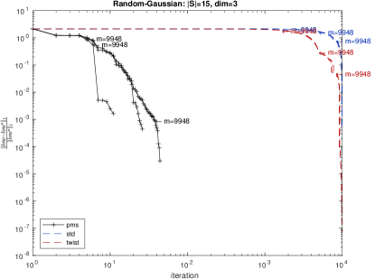
(a) Gaussian

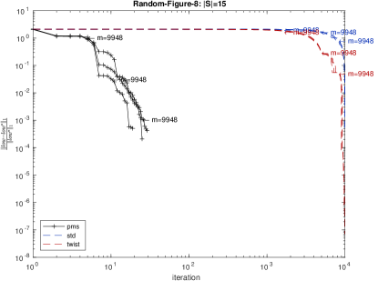
(b) Figure-8

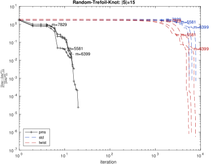
(c) Trefoil Knot

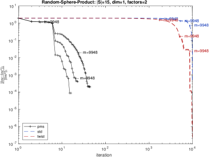
(d) Sphere product

Figure 2: Relative $\ell_{1}$-error per iteration. For each ensemble, three point clouds are sampled and the corresponding simplicial complexes are reduced with each of the algorithms. The relative $\ell_{1}$-error between $\operatorname{low_{\partial}}$ and $\operatorname{low^{*}}$, as given in (23), is tracked.

$\frac{\|\operatorname{low_{\partial}}-\operatorname{low^{*}}\|_{1}}{\|\operatorname{low^{*}}\|_{1}}$	Gaussian			Figure-8			Trefoil-knot			Sphere-product
	pms	std	twist	pms	std	twist	pms	std	twist	pms	std	twist
0.1	14	9786	7366	9	9756	6759	12	7687	5519	7	9751	5589
0.01	20	9933	9180	17	9930	8916	15	7816	7087	10	9930	8485
0.001	24	9948	9197	25	9948	8942	16	7829	7122	13	9948	8564
0.0001	27	9949	9198	26	9949	8944	20	7830	7309	15	9949	9388
0	27	9949	9858	26	9949	9869	21	7830	7732	17	9949	9840

Table 2: Iterations to relative $\ell_{1}$-error. For each ensemble, one point cloud is sampled and the corresponding simplicial complex is reduced with each algorithm. The number of iterations to achieve a given relative $\ell_{1}$-error level between $\operatorname{low_{\partial}}$ and $\operatorname{low^{*}}$, as given by (23), is reported for of Algs. 1 - 3.

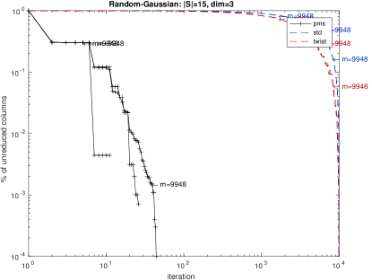
(a) Gaussian

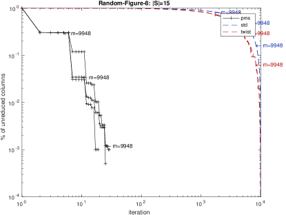
(b) Figure-8

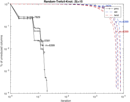
(c) Trefoil Knot

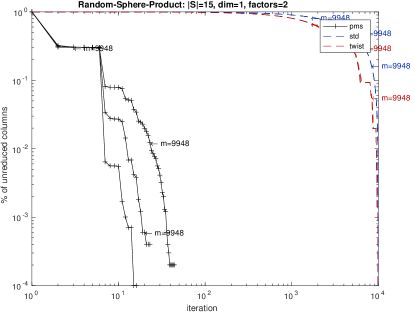
(d) Sphere product

Figure 3: Proportion of unreduced columns per iteration. For each ensemble, three point clouds are sampled and the corresponding simplicial complexes are reduced with each of Algs. 1 - 3. The proportion of unreduced columns is presented at each iteration.

Proportion	Gaussian			Figure-8			Trefoil-knot			Sphere-product
	pms	std	twist	pms	std	twist	pms	std	twist	pms	std	twist
0.90	2	996	528	2	996	499	2	784	392	2	996	519
0.50	2	4975	3405	2	4975	2974	2	3916	2536	2	4975	2958
0.10	12	8955	7424	7	8955	6849	7	7048	6140	7	8955	6115
0.05	15	9452	8432	7	9452	8618	12	7439	6738	7	9452	8404
0.01	20	9850	9471	17	9850	9494	15	7752	7427	7	9850	9461

Table 3: Iterations to unreduced percentage. For each ensemble, one point cloud is sampled and the corresponding simplicial complex is reduced with each of Algs. 1 - 3. The number of iterations to achieve a given proportion of unreduced columns is presented for each algorithm.

4.3 The set $\operatorname{\mathsf{Ess}}$ can be reliably estimated after a few iterations

Finally, we show how the efficacy of Lemma 11 in estimating the the set of essential columns. Let $E^{\ell}$ be defined as in (21), by Lemma 11, $\operatorname{\mathsf{Ess}}\subset E^{\ell}$ for every $\ell$. If $E^{\ell}$ is our estimation at iteration $\ell$, then the number of true positives, false positives and false negatives in the estimation is, respectively,

TP $$=|\operatorname{\mathsf{Ess}}\cap E^{\ell}|=|\operatorname{\mathsf{Ess}}|,$$

FP $$=|E^{\ell}\setminus\operatorname{\mathsf{Ess}}|=|E^{\ell}|-|\operatorname{\mathsf{Ess}}|,$$

FN $$=|\emptyset|=0.$$

To evaluate the quality of the estimation, we compute the precision as defined by

precision $$=\frac{\mbox{TP}}{\mbox{TP}+\mbox{FP}}=\frac{|\operatorname{\mathsf{Ess}}|}{|E^{\ell}|}$$

and note that the recall $=\frac{\mbox{TP}}{\mbox{TP}+\mbox{FN}}$ is equal to 1 due to the estimate giving no false negatives. Fig. 4 and Tab. 4 show the remarkably few iterations needed by Alg. 2 to achieve precision near one while Algs. 1 and 3 show increase in the precision to one only in the later iterations. Specifically, Alg. 2 achieves precision of $95\%$ with two iterations and complete precision within 8 iterations whereas Algs. 1 and 3 require between seven and ten thousand iterations for similar precisions.

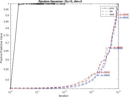
(a) Gaussian

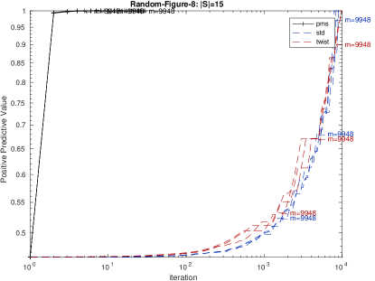
(b) Figure-8

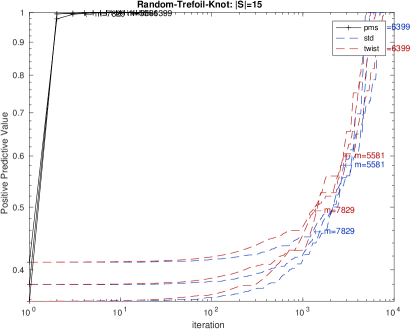
(c) Trefoil Knot

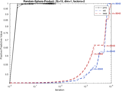
(d) Sphere product

Figure 4: Precision of $\operatorname{\mathsf{Ess}}$ estimation. For each ensemble, three point clouds are sampled and the corresponding simplicial complexes are reduced with each algorithm. At each iteration, $\operatorname{\mathsf{Ess}}$ is estimated and its precision is tracked.

Precision	Gaussian			Figure-8			Trefoil-knot			Sphere-product
	pms	std	twist	pms	std	twist	pms	std	twist	pms	std	twist
0.10	1	1	1	1	1	1	1	1	1	1	1	1
0.50	2	1033	559	2	1231	493	2	2132	1374	2	1016	557
0.90	2	8461	8244	2	7599	8238	2	6691	6445	2	6675	8222
0.95	2	8636	8938	2	7774	8892	2	6871	7123	2	6850	8519
1.00	8	8794	9858	5	7932	9869	8	7004	7732	7	7008	9866

Table 4: Iterations to essential-estimation precision. For each ensemble, one point cloud is sampled and the corresponding simplicial complex is reduced with each algorithm. The number of iterations to achieve a given precision of the set $\operatorname{\mathsf{Ess}}$ is given for each algorithm.

5 Conclusions

We have presented a massively parallel algorithm, Alg. 2 for the reduction of boundary matrices in the scalable computation of persistent homology. This work extends the foundational algorithms bauer2014clear ; chen2011persistent ; edelsbrunner2002topological using many of the same notions, but allowing a dramatically greater distribution of the necessary operations. Our numerical experiments show that Alg 2, as compared with Algs. 1 and 3, is able to pack more operations into few iterations, approximates $\operatorname{low^{*}}$ simultaneously at all scales of the simplicial complex filtration, and determines the essential columns in remarkably few iterations. This massively parallel algorithm suggests the reduction of dramatically larger boundary matrices will now be possible, and moreover allows early termination with accurate results when computational constraints are reached. Implementation of Alg. 2 in the leading software packages, as reported in otter2015roadmap , is underway and we expect to report dramatic reduction in computational times in a subsequent manuscript.

6 Acknowledgements

The authors would like to thank Vidit Nanda for his helpful comments. This work was supported by The Alan Turing Institute under the EPSRC grant EP/N510129/1. RMS acknowledges the support of CONACyT.

References

- [1] Ulrich Bauer, Michael Kerber, and Jan Reininghaus. Clear and compress: Computing persistent homology in chunks. In Topological Methods in Data Analysis and Visualization III, pages 103–117. Springer, 2014.
- [2] Ulrich Bauer, Michael Kerber, and Jan Reininghaus. Distributed computation of persistent homology. In 2014 Proceedings of the Sixteenth Workshop on Algorithm Engineering and Experiments (ALENEX), pages 31–38. SIAM, 2014.
- [3] Gunnar Carlsson. Topology and data. Bulletin of the American Mathematical Society, 46(2):255–308, 2009.
- [4] Gunnar Carlsson. Topological pattern recognition for point cloud data. Acta Numerica, 23:289, 2014.
- [5] Gunnar Carlsson, Tigran Ishkhanov, Vin De Silva, and Afra Zomorodian. On the local behavior of spaces of natural images. International journal of computer vision, 76(1):1–12, 2008.
- [6] Joseph Minhow Chan, Gunnar Carlsson, and Raul Rabadan. Topology of viral evolution. Proceedings of the National Academy of Sciences, 110(46):18566–18571, 2013.
- [7] Chao Chen and Michael Kerber. Persistent homology computation with a twist. In Proceedings 27th European Workshop on Computational Geometry, volume 11, 2011.
- [8] Don Coppersmith and Shmuel Winograd. Matrix multiplication via arithmetic progressions. Journal of symbolic computation, 9(3):251–280, 1990.
- [9] Vin De Silva, Dmitriy Morozov, and Mikael Vejdemo-Johansson. Dualities in persistent (co) homology. Inverse Problems, 27(12):124003, 2011.
- [10] Vin De Silva, Dmitriy Morozov, and Mikael Vejdemo-Johansson. Persistent cohomology and circular coordinates. Discrete & Computational Geometry, 45(4):737–759, 2011.
- [11] Herbert Edelsbrunner and John Harer. Computational topology: an introduction. American Mathematical Soc., 2010.
- [12] Herbert Edelsbrunner, David Letscher, and Afra Zomorodian. Topological persistence and simplification. Discrete and Computational Geometry, 28(4):511–533, 2002.
- [13] Robert Ghrist. Elementary applied topology. Book in preperation, 2014.
- [14] PY Lum, G Singh, A Lehman, T Ishkanov, Mikael Vejdemo-Johansson, M Alagappan, J Carlsson, and G Carlsson. Extracting insights from the shape of complex data using topology. Scientific reports, 3, 2013.
- [15] Rodrigo Mendoza-Smith. Parallel multiscale reduction of ph filtrations. https://github.com/rodrgo/tda, 2017.
- [16] Nikola Milosavljević, Dmitriy Morozov, and Primoz Skraba. Zigzag persistent homology in matrix multiplication time. In Proceedings of the twenty-seventh annual symposium on Computational geometry, pages 216–225. ACM, 2011.
- [17] Dmitriy Morozov. Persistence algorithm takes cubic time in worst case. BioGeometry News, Dept. Comput. Sci., Duke Univ, 2, 2005.
- [18] Monica Nicolau, Arnold J Levine, and Gunnar Carlsson. Topology based data analysis identifies a subgroup of breast cancers with a unique mutational profile and excellent survival. Proceedings of the National Academy of Sciences, 108(17):7265–7270, 2011.
- [19] Nina Otter, Mason A Porter, Ulrike Tillmann, Peter Grindrod, and Heather A Harrington. A roadmap for the computation of persistent homology. arXiv preprint arXiv:1506.08903, 2015.
- [20] Donald R Sheehy. The persistent homology of distance functions under random projection. In Proceedings of the thirtieth annual symposium on Computational geometry, page 328. ACM, 2014.
- [21] Andrew Tausz, Mikael Vejdemo-Johansson, and Henry Adams. JavaPlex: A research software package for persistent (co)homology. In Han Hong and Chee Yap, editors, Proceedings of ICMS 2014, Lecture Notes in Computer Science 8592, pages 129–136, 2014. Software available at http://appliedtopology.github.io/javaplex/.
- [22] Dane Taylor, Florian Klimm, Heather A Harrington, Miroslav Kramár, Konstantin Mischaikow, Mason A Porter, and Peter J Mucha. Topological data analysis of contagion maps for examining spreading processes on networks. Nature communications, 6, 2015.