Characterizing Feshbach resonances in ultracold scattering calculations

Abstract

We describe procedures for converging on and characterizing zero-energy Feshbach resonances that appear in scattering lengths for ultracold atomic and molecular collisions as a function of an external field. The elastic procedure is appropriate for purely elastic scattering, where the scattering length is real and displays a true pole. The regularized scattering length (RSL) procedure is appropriate when there is weak background inelasticity, so that the scattering length is complex and displays an oscillation rather than a pole, but the resonant scattering length $a_{\textrm{res}}$ is close to real. The fully complex procedure is appropriate when there is substantial background inelasticity and the real and imaginary parts of $a_{\textrm{res}}$ are required. We demonstrate these procedures for scattering of ultracold ⁸⁵Rb in various initial states. All of them can converge on and provide full characterization of resonances, from initial guesses many thousands of widths away, using scattering calculations at only about 10 values of the external field.

I Introduction

Zero-energy Feshbach resonances are formed when a bound or quasi-bound state is tuned across a threshold by varying an applied field, most commonly a magnetic field. They are ubiquitous in studies of ultracold physics Chin et al. (2010), where they can be used to tune scattering lengths for many applications, including studies of equations of state Nascimbène et al. (2010), solitons Frantzeskakis (2010), and Efimov physics Kraemer et al. (2006); Huang et al. (2014). They are also used for magnetoassociation to form ultracold molecules Hutson and Soldán (2006); Köhler et al. (2006).

Low-energy scattering may be described by the energy-dependent scattering length $a(E,B)=-k^{-1}\tan\delta$, where $E=\hbar^{2}k^{2}/2\mu$ is the collision energy, $\mu$ is the reduced mass and $\delta$ is the scattering phase shift. This is constant as $E\rightarrow 0$, where it reduces to the usual zero-energy scattering length. At constant energy it is convenient to write $a(E,B)$ as simply $a(B)$. In the simplest case of an isolated narrow resonance without inelastic scattering, $a(B)$ is real and shows a simple pole as a function of applied field $B$. If the background scattering length $a_{\mathrm{bg}}(B)$ is constant across the width of the resonance, the pole is described by Moerdijk et al. (1995)

$$a(B)=a_{\mathrm{bg}}\left(1-\frac{\Delta}{B-B_{\textrm{res}}}\right),$$ (1)

where $B_{\textrm{res}}$ is the position of the resonance, and the width of the resonance is characterized by $\Delta$. The parameters are generally weakly dependent on energy in the threshold region. Obtaining them from quantum scattering calculations based on interaction potentials is an important problem in ultracold collision physics.

It is possible to locate both the pole and the zero of the scattering length and converge on them numerically using standard root-finding algorithms Brue and Hutson (2012); Takekoshi et al. (2012). In the case where $a_{\mathrm{bg}}(B)$ is constant, $\Delta$ is the separation between the pole and the zero. For resonances that are not isolated and narrow, the behavior of the scattering length is more complicated than Eq. (1). Nevertheless, Eq. (1) always holds in some region close to the pole, and the parameters may be defined in terms of this local behavior. When this is done, $a_{\mathrm{bg}}$ may not describe $a(B)$ far from the pole and $\Delta$ may not be precisely the separation between the pole and a zero. Such effects are particularly prominent when there are numerous overlapping resonances Jachymski and Julienne (2013) or when $a_{\mathrm{bg}}$ is small, so that the zero is artificially far from the pole Cho et al. (2013).

If inelastic decay is present then the scattering length is complex Balakrishnan et al. (1997) and its behavior is considerably more complicated. It has no clearly defined zero-crossing, and it no longer shows a pole but instead oscillates with a finite amplitude Hutson (2007); Hutson et al. (2009). This may render decayed resonances unsuitable for tuning scattering lengths to large values Bohn and Julienne (1997). In addition, inelastic rates usually peak sharply near resonance González-Martínez and Hutson (2007), and the resulting losses may make the resonances unsuitable for purposes such as magnetoassociation González-Martínez and Hutson (2013). In other cases, Feshbach resonances can actually reduce inelastic cross sections, which might aid sympathetic cooling Rowlands et al. (2007); Hutson et al. (2009).

In the inelastic case, there is no efficient procedure available to locate and characterize Feshbach resonances. It is in principle possible to obtain resonance parameters by explicit least-squares fitting of S-matrix elements from quantum scattering calculations to appropriate functional forms Ashton et al. (1983). It is also possible to extract an overall width by fitting to the S-matrix eigenphase sum as a function of energy Ashton et al. (1983). This approach has been used for zero-energy Feshbach resonances as a function of magnetic field González-Martínez and Hutson (2007); Rowlands et al. (2007), but it requires large numbers of scattering calculations and substantial manual labor. Better methods are clearly needed.

In this paper we describe efficient, automatable procedures for locating and characterizing zero-energy Feshbach resonances, both in the purely elastic case and in the presence of inelastic scattering. Our algorithms are built on an approach for resonances in purely elastic scattering that we have used previously Cho et al. (2013); Zürn et al. (2013) but have not described in detail. This converges towards a pole using an iterative 3-point fit to calculated scattering lengths. We begin by describing an improved algorithm for this case that converges stably on widths and background scattering lengths as well as pole positions. We then extend the approach to handle the important case when there is inelastic scattering but the inelastic loss away from resonance is small. Finally we deal with the case where there is strong background inelastic scattering. All the methods have been implemented in the general-purpose quantum scattering package molscat Hutson and Le Sueur (2017), and are illustrated here with examples from calculations on collisions of ${}^{85}\textrm{Rb}$ Blackley et al. (2013).

II Elastic scattering

We first describe a reliable general method for converging on and characterizing a resonance in the case of purely elastic scattering. Early versions of this method have been employed in previous work Cho et al. (2013); Zürn et al. (2013), but here we refine it and provide a complete description. We refer to the method described in this section as the elastic procedure.

The elastic procedure uses three calculated scattering lengths $a_{1}$, $a_{2}$ and $a_{3}$ at fields $B_{1}$, $B_{2}$ and $B_{3}$, respectively, close to the resonance. Solving 3 simultaneous equations allows us to extract the three parameters from Eq. (1). Defining

$$\rho=\left(\frac{B_{3}-B_{1}}{B_{2}-B_{1}}\right)\left(\frac{a_{2}-a_{1}}{a_{3}-a_{1}}\right),$$ (2)

we obtain

$$B_{\textrm{res}} =\frac{B_{3}-B_{2}\rho}{1-\rho}$$ (3)

$$a_{\textrm{bg}}\Delta =\frac{(B_{3}-B_{\textrm{res}})(B_{1}-B_{\textrm{res}})(a_{3}-a_{1})}{B_{3}-B_{1}}$$ (4)

and finally

$$a_{\textrm{bg}}=a_{1}+\frac{a_{\textrm{bg}}\Delta}{B_{1}-B_{\textrm{res}}}.$$ (5)

In order to iterate and converge towards the pole we must not only choose a point for a new scattering calculation but also choose which of the previous three results to discard. The obvious choice for a new point is the estimated $B_{\textrm{res}}$, but this causes points to pile up close to the pole, and Eqs. (2) to (5) are numerically unstable when 2 points are very close together. We therefore choose the new point with the aim that the final three points should include one point very close to the pole, one point between $t_{\textrm{min}}\Delta$ and $2t_{\textrm{min}}\Delta$ from the pole, and one point between $t_{\textrm{max}}\Delta$ and $2t_{\textrm{max}}\Delta$ from the pole on the opposite side. These three points can be thought of as allowing characterization of $B_{\textrm{res}}$, $a_{\textrm{bg}}\Delta$, and $a_{\rm bg}$, respectively. The tolerances $t_{\textrm{min}}$ and $t_{\textrm{max}}$ are positive, with $t_{\textrm{min}}<t_{\textrm{max}}$. The values $t_{\textrm{min}}=0.1$ and $t_{\textrm{max}}=1.0$ are almost always appropriate for isolated resonances; we use these values throughout this paper, but different choices may be appropriate in other cases. We terminate the iteration when the estimated value of $B_{\textrm{res}}$ is within a small amount $\epsilon$ of the closest of the 3 points and the other two points satisfy the criteria above. The logic we have implemented to select which point to discard and where to place the next point is shown in Fig. 1.

Figure 1: Flowchart representation of the algorithm to select which point to discard and where to place the next point.

We need 3 fields in the vicinity of the resonance to start the procedure. We choose to use equally spaced points separated by a small amount $\delta B$; in this work we choose this value to be 0.2 G. The algorithm will, of course, perform best when one of the initial points is close to the pole, but in this paper we choose points such that the pole is approximately at the midpoint of two of them to provide the strictest test of the procedure. In practice, the initial estimate of the pole position could come from a number of different sources such as scattering calculations on a grid or calculations of the bound states of the system; we usually use the program field Hutson (2011) which can directly calculate fields at which there is a bound state exactly at threshold.

Table 1: Convergence towards the resonance near 171 G for two ⁸⁵Rb atoms in their $F=2,M_{F}=2$ state. Units are G and the Bohr radius $a_{0}$.

Resonance near $B_{\textrm{ref}}=171.561$ G
				Estimated values
$n$	$B_{n}-B_{\textrm{ref}}$	$(B_{n}-B_{\textrm{res}})/\Delta$	$a$	$B_{\textrm{res}}-B_{\textrm{ref}}$	$\Delta$	$a_{\textrm{bg}}$	$a_{\textrm{bg}}\Delta$
$1$	$-1.00227\times 10^{-1}$	$4.24\times 10^{3}$	$-438.67$	-	-	-	-
$2$	$2.99773\times 10^{-1}$	$-1.27\times 10^{4}$	$-438.76$	-	-	-	-
$3$	$9.97730\times 10^{-2}$	$-4.24\times 10^{3}$	$-438.85$	$3.40045\times 10^{-2}$	$-1.8427\times 10^{-5}$	$-438.73$	$8.0846\times 10^{-3}$
$4$	$3.40045\times 10^{-2}$	$-1.45\times 10^{3}$	$-439.06$	$3.68297\times 10^{-3}$	$-2.0840\times 10^{-5}$	$-438.75$	$9.1437\times 10^{-3}$
$5$	$3.68297\times 10^{-3}$	$-166$	$-441.40$	$-3.79856\times 10^{-4}$	$-2.4633\times 10^{-5}$	$-438.74$	$1.0807\times 10^{-2}$
$6$	$-3.79856\times 10^{-4}$	$6.49$	$-371.13$	$-2.26739\times 10^{-4}$	$-2.3598\times 10^{-5}$	$-438.75$	$1.0354\times 10^{-2}$
$7$	$-2.26739\times 10^{-4}$	$-0.00989$	$-44657$	$-2.26973\times 10^{-4}$	$-2.3563\times 10^{-5}$	$-438.76$	$1.0339\times 10^{-2}$
$8$	$-2.23438\times 10^{-4}$	$-0.150$	$-3364.4$	$-2.26973\times 10^{-4}$	$-2.3568\times 10^{-5}$	$-438.77$	$1.0341\times 10^{-2}$
$9$	$-2.62324\times 10^{-4}$	$1.50$	$-146.31$	$-2.26973\times 10^{-4}$	$-2.3565\times 10^{-5}$	$-438.82$	$1.0341\times 10^{-2}$
$10$	$-2.26973\times 10^{-4}$	$4.24\times 10^{-5}$	$1.631\times 10^{7}$	$-2.26972\times 10^{-4}$	$-2.3564\times 10^{-5}$	$-438.76$	$1.0339\times 10^{-2}$

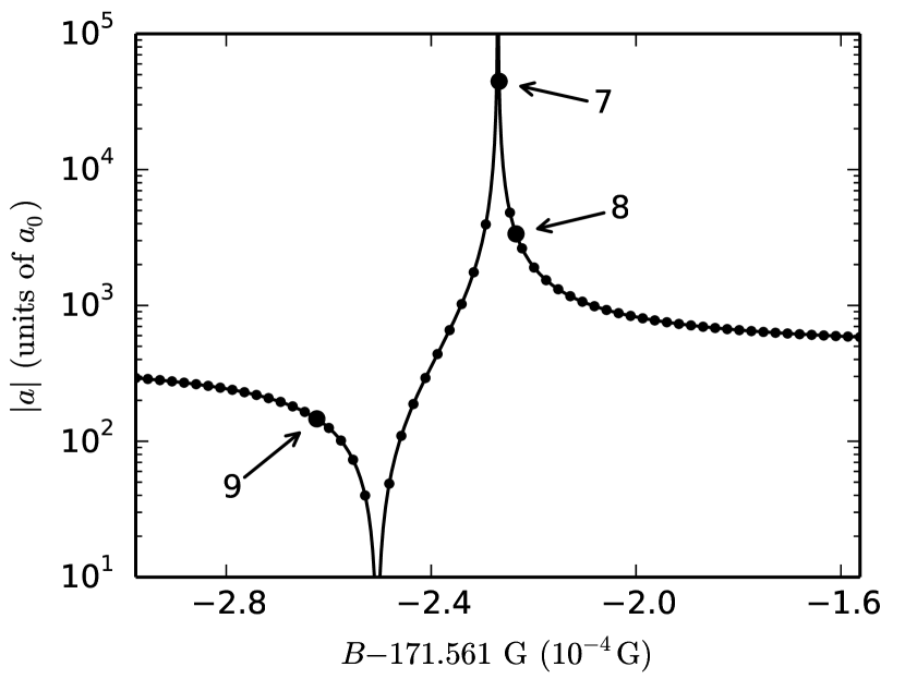
Figure 2: Convergence towards the elastic resonance near 171 G for two ⁸⁵Rb atoms in their $F=2,M_{F}=2$ state. Note the logarithmic vertical scale. The filled circles show the results of scattering calculations of $|a|$ at the sequence of points $n$ produced by the elastic procedure; the black line shows Eq. (1) with the final estimated parameters; and the small dots show scattering calculations on a grid for comparison.

To demonstrate the convergence of this method, we apply it to a resonance near 171 G in collisions of two ⁸⁵Rb atoms in their lowest ($F=2,M_{F}=2$) state. Scattering lengths are calculated using the molscat package, as described by Blackley et al. Blackley et al. (2013), at energy $E=1\ \textrm{nK}\times k_{\textrm{B}}$. We choose $\epsilon=10^{-9}$ G, which is limited by noise in our scattering calculations. Table 1 summarizes the convergence towards the resonance, with the parameters estimated by Eqs. (2) to (5) at each iteration; Figure 2 provides a graphical representation of the convergence process. This resonance is narrow, with $\Delta=2.3\times 10^{-5}$ G, yet our method successfully converges rapidly on the pole even though the closest of the 3 initial points is over 4000 widths away. The 8th and 9th points are actually placed away from the pole by the algorithm to satisfy the requirements associated with $t_{\textrm{min}}$ and $t_{\textrm{max}}$ before the final point is placed extremely close to the pole. The entire procedure needs only 10 scattering calculations and requires no human intervention after the initial set of points; a corresponding manual search and subsequent least-squares fit would have needed many more scattering calculations and considerable human input.

If the pole position $B_{\textrm{res}}$ is all that is required, and $\Delta$ and $a_{\textrm{bg}}$ are unimportant, then the fastest convergence is often achieved by setting $t_{\textrm{min}}=t_{\textrm{max}}=0$. With this choice, the present algorithm reduces to that used in previous work from our group Cho et al. (2013); Zürn et al. (2013). The equations for $\Delta$ and $a_{\textrm{bg}}$ then become unstable as convergence proceeds and the points cluster close to the pole, but $B_{\textrm{res}}$ usually converges smoothly.

All the algorithms described here make the approximation that $a_{\textrm{bg}}(B)$ is constant across the range of points. This approximation improves as the convergence proceeds and the range of points becomes smaller. Nevertheless, it is the limiting factor that determines the distance from which convergence can be achieved. At least one of the initial points must give a scattering length that is affected by the resonance by more than the variation of $a_{\textrm{bg}}(B)$ across the range of the points. For very narrow resonances, computational noise in the scattering length can also affect convergence.

III Inelastic scattering

In the presence of inelastic loss, the diagonal S-matrix element in the incoming channel $S_{00}=\exp(2\textrm{i}\delta)$ has magnitude less than 1. The phase shift $\delta$ is thus complex, and so is the scattering length $a=\alpha-\textrm{i}\beta$, where $\beta\geq 0$ Balakrishnan et al. (1997). The real and imaginary parts of the scattering length characterize the elastic and inelastic cross sections, respectively. The energy-dependent scattering length may be written exactly as Hutson (2007)

$$a(E,B)=\frac{-\tan\delta(E,B)}{k}=\frac{1}{\textrm{i}k}\left(\frac{1-S_{00}(E,B)}{1+S_{00}(E,B)}\right).$$ (6)

Around a resonance, the scattering length at constant energy describes a circle in the complex plane Hutson (2007), beginning and ending at the background scattering length $a_{\textrm{bg}}$,

$$a(B)=a_{\textrm{bg}}+\frac{a_{\textrm{res}}}{2(B-B_{\textrm{res}})/\Gamma_{B}^{\textrm{inel}}+\textrm{i}}.$$ (7)

$a_{\textrm{bg}}=\alpha_{\textrm{bg}}-\textrm{i}\beta_{\textrm{bg}}$ is now complex and $a_{\textrm{res}}=\alpha_{\textrm{res}}-\textrm{i}\beta_{\textrm{res}}$ is a ‘resonant’ scattering length that describes the size and direction of the circle. $\Gamma_{B}^{\textrm{inel}}$ is a decay width for the quasibound state that causes the resonance; it is a real quantity, with dimensions of field, whose sign depends on the magnetic moment of the state relative to the threshold. It is useful to identify

$$\alpha_{\textrm{res}}\Gamma_{B}^{\textrm{inel}}=-2\alpha_{\textrm{bg}}\Delta$$ (8)

to allow a connection back to Eq. (1), although $\Delta$ no longer has a simple interpretation as the distance between the pole and zero in $a$.

Around a decayed resonance, both $\alpha$ and $\beta$ show an oscillation, determined by $a_{\textrm{res}}$, rather than a pole Hutson (2007); Rowlands et al. (2007); Hutson et al. (2009). This has implications for the observation and use of such resonances Bohn and Julienne (1997); González-Martínez and Hutson (2007, 2013). In the very common case $|a_{\textrm{res}}|\gg\beta_{\textrm{bg}}$, $\beta(B)$ displays a peak of magnitude $a_{\textrm{res}}$. However, $a_{\textrm{res}}$ is inversely proportional to $\Gamma_{B}^{\textrm{inel}}$. Somewhat counterintuitively, therefore, weaker inelastic decay of the quasibound state responsible for the resonance causes a higher peak in $\beta(B)$ (and hence in the inelastic rate) around $B_{\textrm{res}}$.

III.1 Weak background inelasticity

We first consider the important case where the background inelasticity can be neglected, so we approximate $\beta_{\textrm{bg}}=0$. Under this approximation $a_{\textrm{res}}$ is also real Rowlands et al. (2007), though $a(B)$ itself remains complex near resonance. There are thus only 4 parameters to extract. Even so, Eq. (7) does not allow us to extract parameters as easily as we could from Eq. (1). However, this can be overcome by defining a ‘regularized scattering length’

$$\mathcal{A} =\alpha+\frac{\beta^{2}}{\alpha-\alpha_{\textrm{bg}}}$$ (9)

$$=\alpha_{\textrm{bg}}-\frac{\alpha_{\textrm{bg}}\Delta}{B-B_{\textrm{res}}}.$$ (10)

which is real and shows a simple pole just like Eq. (1). This allows us to use Eqs. (2) to (5) with $a$ replaced by $\mathcal{A}$ to extract three of the parameters and converge on the resonance position as before, with minimal modification of the elastic procedure. We refer to the resulting method as the regularized scattering length (RSL) procedure.

The final parameter $a_{\textrm{res}}$ can be estimated at each stage of the convergence using the identity,

$$a_{\textrm{res}}=\frac{|a-a_{\textrm{bg}}|^{2}}{\beta}=\beta+\frac{(\alpha-\alpha_{\textrm{bg}})^{2}}{\beta}.$$ (11)

In the important case where $\Gamma_{B}^{\textrm{inel}}$ is very small, the peak in $\beta$ is very narrow. Estimating $a_{\textrm{res}}$ from the maximum value of $\beta$ can thus be very difficult, but Eq. (11) provides a useful estimate as soon as both $\alpha$ and $\beta$ differ significantly from their background values. Equations (9) and (11) each need an estimate of $\alpha_{\textrm{bg}}$. This can be obtained iteratively, but we find that in practice it is adequate to take it from the previous or current iteration, respectively. To calculate $\mathcal{A}$ at the first iteration we use the average of $a_{1}$ and $a_{2}$ as an initial approximation for $a_{\textrm{bg}}$. Equation (11) can also be used separately from the convergence algorithm employed here, for example to estimate $a_{\textrm{res}}$ from scattering calculations on a grid that is not fine enough to resolve the peak in $\beta$.

Table 2: Convergence towards resonances with weak background inelasticity for two ⁸⁵Rb atoms in their $F=2,M_{F}=-2$ state. Units are G and the Bohr radius $a_{0}$.

Resonance near $B_{\textrm{ref}}=215.084$ G
						Estimated values
$n$	$B_{n}-B_{\textrm{ref}}$	$(B_{n}-B_{\textrm{res}})/\Delta$	$\alpha_{n}$	$\beta_{n}$	$\mathcal{A}_{n}$	$B_{\textrm{res}}-B_{\textrm{ref}}$	$\Delta$	$a_{\textrm{bg}}$	$a_{\textrm{res}}$
$1$	$-9.96246\times 10^{-2}$	$-18.0$	$-402.1$	$0.000796$	$-402.1$	-	-	-	-
$2$	$3.00375\times 10^{-1}$	$53.9$	$-374.5$	$0.000692$	$-374.5$	-	-	-	-
$3$	$1.00375\times 10^{-1}$	$18.0$	$-360.0$	$0.000649$	$-360.0$	$2.81284\times 10^{-3}$	$5.514\times 10^{-3}$	$-381.53$	$7.168\times 10^{5}$
$4$	$2.81284\times 10^{-3}$	$0.438$	$489.6$	$0.00219$	$489.6$	$3.95129\times 10^{-4}$	$5.524\times 10^{-3}$	$-381.02$	$3.459\times 10^{8}$
$5$	$3.95129\times 10^{-4}$	$0.00354$	$1.07\times 10^{5}$	$67.6$	$1.07\times 10^{5}$	$3.75429\times 10^{-4}$	$5.568\times 10^{-3}$	$-381.19$	$1.716\times 10^{8}$
$6$	$-7.97622\times 10^{-3}$	$-1.50$	$-635.1$	$0.00197$	$-635.1$	$3.75433\times 10^{-4}$	$5.569\times 10^{-3}$	$-381.01$	$1.716\times 10^{8}$
$7$	$1.21083\times 10^{-3}$	$0.150$	$2159$	$0.0299$	$2159$	$3.75433\times 10^{-4}$	$5.569\times 10^{-3}$	$-381.00$	$1.716\times 10^{8}$
$8$	$3.75433\times 10^{-4}$	$-1.80\times 10^{-7}$	$-1.32\times 10^{7}$	$1.70\times 10^{8}$	$-2.19\times 10^{9}$	$3.75434\times 10^{-4}$	$5.569\times 10^{-3}$	$-381.00$	$1.707\times 10^{8}$
Resonance near $B_{\textrm{ref}}=603.977$ G
$1$	$-9.93851\times 10^{-2}$	$-531$	$-476.7$	$0.00159$	$-476.7$	-	-	-	-
$2$	$3.00615\times 10^{-1}$	$1.59\times 10^{3}$	$-475.6$	$1.39\times 10^{-5}$	$-475.6$	-	-	-	-
$3$	$1.00615\times 10^{-1}$	$531$	$-475.0$	$0.000630$	$-475.0$	$1.08784\times 10^{-2}$	$1.7996\times 10^{-4}$	$-475.91$	$1.446\times 10^{3}$
$4$	$1.08784\times 10^{-2}$	$54.5$	$-467.1$	$0.0954$	$-467.1$	$9.67212\times 10^{-4}$	$1.8191\times 10^{-4}$	$-475.82$	$7.991\times 10^{2}$
$5$	$9.67212\times 10^{-4}$	$1.87$	$-246.8$	$76.3$	$-221.4$	$6.13682\times 10^{-4}$	$1.8905\times 10^{-4}$	$-475.86$	$7.635\times 10^{2}$
$6$	$6.13682\times 10^{-4}$	$-0.00659$	$-483.8$	$762$	$-7.32\times 10^{4}$	$6.14914\times 10^{-4}$	$1.8838\times 10^{-4}$	$-475.82$	$7.621\times 10^{2}$
$7$	$5.86657\times 10^{-4}$	$-0.150$	$-648.9$	$720$	$-3647$	$6.14919\times 10^{-4}$	$1.8837\times 10^{-4}$	$-475.81$	$7.621\times 10^{2}$
$8$	$6.14919\times 10^{-4}$	$-2.65\times 10^{-5}$	$-475.8$	$762$	$-1.84\times 10^{7}$	$6.14924\times 10^{-4}$	$1.8838\times 10^{-4}$	$-475.83$	$7.621\times 10^{2}$

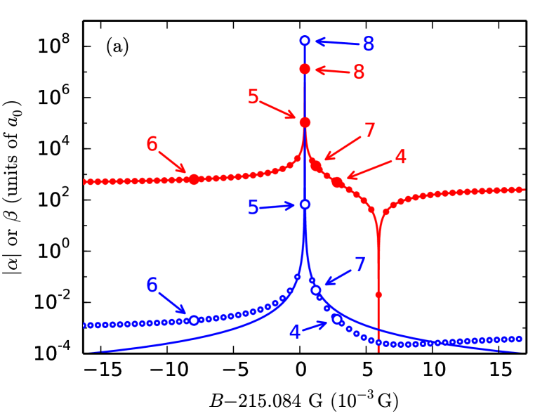
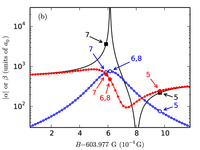
Figure 3: Convergence towards resonances with weak background inelasticity for two ⁸⁵Rb atoms in their $F=2,M_{F}=-2$ state. (a) Resonance near 215 G; (b) Resonance near 604 G. The large symbols show values of $|\alpha|$ (red, filled circles) and $\beta$ (blue, open circles) from scattering calculations at the sequence of points $n$ produced by the RSL procedure; the fitted functions are shown as corresponding lines through the symbols; the small dots show scattering calculations on a grid for comparison. The black squares and line in (b) show the regularized scattering length $\mathcal{A}$.

Table 2 summarizes the convergence towards two resonances in collisions of a pair of ⁸⁵Rb atoms in their $F=2,M_{F}=-2$ excited state, using the RSL procedure. These results are also shown in Fig. 3. These collisions are weakly inelastic away from resonances, because loss comes only from spin-relaxation transitions driven by the weak dipole-dipole interaction. We use a slightly larger value for the convergence criterion than in the previous section, $\epsilon=10^{-8}$ G.

The first inelastic resonance we analyze, near 215 G, shows only weak inelastic decay, as seen from the small values of $\beta$ and negligible differences between $\alpha$ and $\mathcal{A}$ except at the final point. The RSL procedure converges smoothly and provides stable values of all the resonance parameters. The fitted $\beta(B)$ is shown in Fig. 3(a); it is accurate near the center of the resonance, but deviates from the calculated values by a small amount in the wings because the actual background $\beta_{\textrm{bg}}$ is non-zero. As described above, the RSL procedure provides an estimate $a_{\textrm{res}}=1.7\times 10^{8}$ $a_{0}$ that is stable over the final few iterations even when $\beta$ is 6 orders of magnitude smaller than $a_{\textrm{res}}$; the final calculation confirms that these estimates of $a_{\textrm{res}}$ are remarkably accurate. For this resonance, the elastic procedure would work well until the last point, when it would predict a pole position some distance away from the resonance. The elastic procedure would thus fail to converge, and continue indefinitely, repeatedly approaching the resonance and jumping away again.

The second resonance we analyze, near 604 G, is quite strongly decayed. The pole in $\alpha$ is strongly suppressed, to the point that $\alpha$ does not even cross zero. By contrast, the regularized scattering length still has a pole and zero crossing as before. The elastic procedure would fail completely anywhere near the center of the resonance, but with the modification of Eq. (9) we can efficiently converge to the resonance position. The final fitted $\alpha(B)$ and $\beta(B)$, shown in Fig. 3(b), agree very well with the calculated values, demonstrating that the resonance has been accurately characterized. The new fitted value of $\Delta=1.8\times 10^{-4}$ G is two orders of magnitude smaller than the value reported previously Blackley et al. (2013), which was obtained by fitting $\alpha(B)$ to Eq. (1) far from resonance.

III.2 Strong background inelasticity

Finally, we consider the case with background inelasticity included. There are now a total of 6 parameters required to characterize a resonance according to Eq. (7): $B_{\textrm{res}}$, $\Gamma_{B}^{\textrm{inel}}$, and the real and imaginary parts of $a_{\textrm{bg}}$ and $a_{\textrm{res}}$. However, each value of $a(B)$ has real and imaginary parts, so we again need scattering calculations at only three fields.

We begin by locating the scattering length at the center of the circle described by Eq. (7), $a_{\textrm{c}}=a_{\textrm{bg}}-\textrm{i}a_{\textrm{res}}/2$. Starting from the equation for a circle, $(\alpha_{n}-\alpha_{\textrm{c}})^{2}+(\beta_{n}-\beta_{\textrm{c}})^{2}=R^{2}$, it is straightforward to derive the simultaneous equations

$$\begin{pmatrix}\alpha_{2}-\alpha_{1}&\beta_{2}-\beta_{1}\\ \alpha_{3}-\alpha_{2}&\beta_{3}-\beta_{2}\end{pmatrix}\begin{pmatrix}\alpha_{\textrm{c}}\\ \beta_{\textrm{c}}\end{pmatrix}=\frac{1}{2}\begin{pmatrix}|a_{2}|^{2}-|a_{1}|^{2}\\ |a_{3}|^{2}-|a_{2}|^{2}\end{pmatrix}.$$ (12)

These are solved to obtain $a_{\textrm{c}}$ and $R=|a_{n}-a_{\textrm{c}}|=|a_{\textrm{res}}|/2$. Across the resonance, the angle $\theta$ around this circle is described by a Breit-Wigner phase,

$$\frac{\theta}{2}=\frac{\theta_{\textrm{bg}}}{2}+\arctan\left(\frac{\Gamma^{\rm inel}}{2(B_{\textrm{res}}-B)}\right).$$ (13)

We define the dimensionless quantity

$$\widetilde{a}(B)=\tan\frac{\theta}{2}=\tan\left(\frac{\arg(a(B)-a_{\textrm{c}})}{2}\right),$$ (14)

which has a pole analogous to Eq. (1). We evaluate $\widetilde{a}_{1}$, $\widetilde{a}_{2}$ and $\widetilde{a}_{3}$ at $B_{1}$, $B_{2}$ and $B_{3}$ and use Eqs. (2) to (5) to obtain parameters $\widetilde{B}_{\textrm{res}}$, $\widetilde{\Delta}$, and $\widetilde{a}_{\textrm{bg}}$ (which do not have immediate physical interpretations). $\widetilde{a}_{\textrm{bg}}=\tan(\theta_{\textrm{bg}}/2)$ tells us where on the circle $a_{\textrm{bg}}$ lies,

$$a_{\textrm{bg}}=a_{\textrm{c}}+R\exp(\textrm{i}\theta_{\textrm{bg}})$$ (15)

and therefore

$$a_{\textrm{res}}=2\textrm{i}(a_{\textrm{c}}-a_{\textrm{bg}}).$$ (16)

$a(B_{\textrm{res}})$ is diametrically opposite $a_{\textrm{bg}}$ on the circle, so

$$\widetilde{a}(B_{\textrm{res}})=\tan\left(\frac{\theta_{\textrm{bg}}+\pi}{2}\right)=-\frac{1}{\widetilde{a}_{\textrm{bg}}}.$$ (17)

We then obtain $B_{\textrm{res}}$ from

$$B_{\textrm{res}}=\widetilde{B}_{\textrm{res}}-\frac{\widetilde{a}_{\textrm{bg}}\widetilde{\Delta}}{\widetilde{a}(B_{\textrm{res}})-\widetilde{a}_{\textrm{bg}}}=\widetilde{B}_{\textrm{res}}+\frac{\widetilde{\Delta}}{1+\widetilde{a}_{\textrm{bg}}^{-2}}.$$ (18)

Finally, we obtain $\Gamma_{B}^{\textrm{inel}}$ from one calculated scattering length using Eq. (7).

This procedure provides an estimate of $B_{\textrm{res}}$ and other parameters from calculations of $a(B)$ at a set of 3 points. We iterate using the algorithm described in section II, but using the larger of $\Gamma_{B}^{\textrm{inel}}$ and $\Delta$ to constrain the separation of the points from $B_{\textrm{res}}$. We refer to the resulting method as the fully complex procedure.

To demonstrate this, we consider convergence towards a resonance near 172 G in collisions of two ⁸⁵Rb atoms in their $F=3,M_{F}=2$ excited state. In this case the atoms can decay through spin-exchange collisions, which cause faster inelastic loss away from resonance than in Sec. III A. The convergence is summarized in Table 3 and shown in Fig. 4, using $\epsilon=10^{-7}$ G. The procedure converges rapidly on the resonance position and the final fitted functions show excellent agreement with the calculated scattering lengths. The resonance is very strongly decayed; $|a_{\textrm{res}}|$ is less than $5\ a_{0}$ and has a substantial imaginary component. This makes the oscillations in $\alpha(B)$ and $\beta(B)$ somewhat asymmetric.

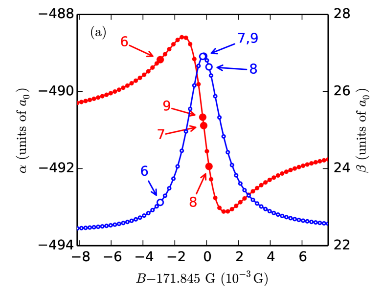
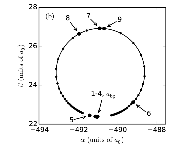
Figure 4: Convergence towards the resonance near 172 G for two ⁸⁵Rb atoms in their $F=3,M_{F}=2$ state. (a) $\alpha$ (red, filled circles) and $\beta$ (blue, open circles) from scattering calculations at the sequence of points $n$ produced by the fully complex procedure; the fitted functions are shown as corresponding lines through the symbols; the small dots show scattering calculations on a grid for comparison. (b) The circle described by $a(B)=\alpha(B)-\textrm{i}\beta(B)$ in the complex plane.

Table 3: Convergence towards the resonance near 172 G for two ⁸⁵Rb atoms in their $F=3,M_{F}=2$ state. Units are G and the Bohr radius $a_{0}$.

Resonance near $B_{\textrm{ref}}=171.845$ G
					Estimated values
$n$	$B_{n}-B_{\textrm{ref}}$	$(B_{n}-B_{\textrm{res}})/\Delta$	$\alpha_{n}$	$\beta_{n}$	$B_{\textrm{res}}-B_{\textrm{ref}}$	$\Gamma_{B}^{\textrm{inel}}$	$\alpha_{\textrm{bg}}$	$\beta_{\textrm{bg}}$	$\alpha_{\textrm{res}}$	$\beta_{\textrm{res}}$
$1$	$-1.00244\times 10^{-1}$	$38.0$	$-490.99$	$22.388$	-	-	-	-	-	-
$2$	$2.99756\times 10^{-1}$	$-114$	$-491.02$	$22.371$	-	-	-	-	-	-
$3$	$9.97560\times 10^{-2}$	$-38.0$	$-491.09$	$22.386$	$6.92055\times 10^{-2}$	$-4.7788\times 10^{-2}$	$-491.01$	$22.377$	$0.10979$	$0.065852$
$4$	$6.92055\times 10^{-2}$	$-26.4$	$-491.12$	$22.391$	$1.58950\times 10^{-2}$	$-1.2632\times 10^{-2}$	$-491.03$	$22.384$	$0.71330$	$0.026746$
$5$	$1.58950\times 10^{-2}$	$-6.14$	$-491.40$	$22.446$	$-2.91246\times 10^{-3}$	$-1.5078\times 10^{-3}$	$-491.01$	$22.376$	$9.7150$	$-1.3474$
$6$	$-2.91246\times 10^{-3}$	$1.01$	$-489.17$	$23.122$	$-1.80823\times 10^{-4}$	$-2.7312\times 10^{-3}$	$-491.03$	$22.382$	$4.4502$	$-0.37429$
$7$	$-1.80823\times 10^{-4}$	$-0.0241$	$-490.88$	$26.918$	$-2.43111\times 10^{-4}$	$-2.6270\times 10^{-3}$	$-491.04$	$22.386$	$4.5243$	$-0.36788$
$8$	$1.50937\times 10^{-4}$	$-0.150$	$-491.94$	$26.638$	$-2.44221\times 10^{-4}$	$-2.6291\times 10^{-3}$	$-491.04$	$22.387$	$4.5232$	$-0.37363$
$9$	$-2.44221\times 10^{-4}$	$1.75\times 10^{-6}$	$-490.67$	$26.910$	$-2.44216\times 10^{-4}$	$-2.6290\times 10^{-3}$	$-491.04$	$22.387$	$4.5232$	$-0.37361$

The fully complex procedure can also resolve the discrepancy between the calculated $\beta(B)$ and the fitted function far from resonance in Fig. 3(a). Figure 5 shows the results of the fully complex procedure in this case, and it may be seen that excellent agreement is obtained. The converged values of the parameters are very similar to those in Table 2, with the addition of $\beta_{\textrm{bg}}=7.20\times 10^{-4}\ a_{0}$ and $\beta_{\textrm{res}}=-582\ a_{0}$.

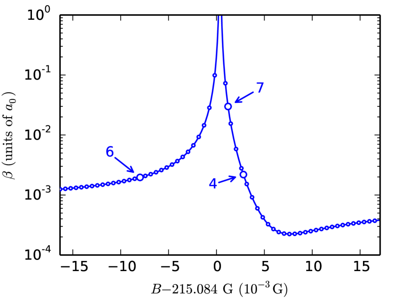
Figure 5: Convergence towards the resonance near 215 G for two ⁸⁵Rb atoms in their $F=2,M_{F}=-2$ state using the fully complex procedure. Only $\beta$ is shown and the axis is expanded to show the asymmetry clearly. Symbols and lines are as in previous figures.

For this procedure to converge well, the circle in the complex plane described by $a(B)$ must be well formed. Variation of $a_{\textrm{bg}}(B)$ across the width of the resonance can distort the circle; if this distortion is significant compared to the size of the circle, the procedure may fail. This leads to the criterion

$$\left|\frac{da_{\textrm{bg}}}{dB}\Gamma_{B}^{\textrm{inel}}\right|\ll|a_{\textrm{res}}|.$$ (19)

The procedure may thus be unsuitable for the widest and most strongly decayed resonances (large $\Gamma_{B}^{\textrm{inel}}$ and small $a_{\textrm{res}}$). The procedure may also fail for overlapping resonances. These restrictions are similar to the criteria used to define an isolated narrow resonance Ashton (1981); Ashton et al. (1983).

IV Conclusions

In this paper we have developed three procedures for efficiently and accurately converging on and characterizing different kinds of zero-energy Feshbach resonances as a function of external field. These procedures can converge on and accurately characterize resonances, from initial guesses many thousands of widths away, with a total of only around 10 scattering calculations.

First we have described the elastic procedure. This is designed for resonances in purely elastic scattering, where the scattering length has a true pole. At each iteration, the procedure characterizes the resonance using scattering calculations at 3 values of the external field, while ensuring that the points do not cluster too close to the pole. This allows stable evaluation of the width and background scattering length as well as the pole position.

For the case of weak background inelasticity we have developed the regularized scattering length (RSL) procedure. The oscillation in the complex scattering length is converted into a true pole in a “regularized” scattering length, and convergence on the pole is achieved in the same way as in the elastic procedure. We also provide a means to estimate the resonant scattering length $a_{\textrm{res}}$ from calculations in the wings of the resonance.

Finally, we have developed a fully complex procedure to converge on and extract all 6 parameters needed to characterize resonances when there is substantial background inelasticity and the real and imaginary parts of $a_{\textrm{res}}$ are required.