Electron $g$-factor of valley states in realistic silicon quantum dots

Abstract

We theoretically model the spin-orbit interaction in silicon quantum dot devices, relevant for quantum computation and spintronics. Our model is based on a modified effective mass approach which properly accounts for spin-valley boundary conditions, derived from the interface symmetry, and should have applicability for other heterostructures. We show how the valley-dependent interface-induced spin-orbit 2D (3D) interaction, under the presence of an electric field that is perpendicular to the interface, leads to a g-factor renormalization in the two lowest valley states of a silicon quantum dot. These g-factors can change with electric field in opposite direction when intervalley spin-flip tunneling is favored over intra-valley processes, explaining recent experimental results. We show that the quantum dot level structure makes only negligible higher order effects to the g-factor. We calculate the g-factor as a function of the magnetic field direction, which is sensitive to the interface symmetry. We identify spin-qubit dephasing sweet spots at certain directions of the magnetic field, where the g-factor renormalization is zeroed: these include perpendicular to the interface magnetic field, and also in-plane directions, the latter being defined by the interface-induced spin-orbit constants. The g-factor dependence on electric field opens the possibility for fast all-electric manipulation of an encoded, few electron spin-qubit, without the need of a nanomagnet or a nuclear spin-background. Our approach of an almost fully analytic theory allows for a deeper physical understanding of the importance of spin-orbit coupling to silicon spin qubits.

I Introduction

Electronic $g$-factor arises as a direct consequence of the spin-orbit coupling (SOC); while relativistic in origin, SOC can be considerably modified in solids due to the electron’s quasiparticle nature and a non-trivial band structure, as well as a result of heterostructure confinement effects (see, e.g. Ref. Rashba and Sheka, 1991). The variations of $g$-factor (and more generally, a SOC) in heterostructures and compounds in externally applied electric or magnetic fields is at the basis of spintronics and has led to a multitude of exotic proposals, ranging from spin-transistors Datta and Das (1990) to topological insulators Hasan and Kane (2010). While the SOC interaction is often considered in novel materials, it turns out to be a non-negligible effect in silicon as well Jansen (2012). As silicon is recognized as a promising material for spin-based quantum computing Zwanenburg et al. (2013), understanding the manifiestation and influence of SOC in real devices takes on increased importance. Particularly relevant are lateral quantum dots (QD) realized in silicon heterostructures confining few electrons, which allow electric gate control of the spin system Maune et al. (2012); Yang et al. (2013); Hao et al. (2014); Kim et al. (2014); Kawakami et al. (2014); Veldhorst et al. (2014, 2015a, 2015b); Ferdous et al. (2018a, b); Jock et al. (2018); Corna et al. (2018); Tanttu et al. (2018). Silicon can be isotopically enriched to ²⁸Si and chemically purified, (see, e.g. Ref.Itoh and Watanabe (2014)), thus removing nuclear spin background as a major source of spin qubit dephasing. As a consequence of the increased qubit sensitivity to variations in resonance frequency, the $g$-factor’s (weak) tunability with an applied electric field becomes an appreciable tool for qubit manipulationKawakami et al. (2014); Veldhorst et al. (2014, 2015b, 2015a).

The standard description of the $g$-factor renormalization in a crystal is via a second-order perturbation theory (PT), using the bulk $\bm{k}\cdot\bm{p}$ Hamiltonian ${\cal H}(\bm{k})$ plus the spin-orbit interaction. It is given as a sum over the virtual electronic excited states (bands), where a relative contribution of an excited state depends on its coupling to the electron state of interest via the spin-orbit interaction Hamiltonian, and is suppressed by the corresponding energy denominatorRoth (1960). In Si, however, the bulk renormalization is very weak (of the order of $\delta g\sim 10^{-3}$), explained theoretically Roth (1960); Liu (1962) by the large band-gap at the six equivalent conduction-band minima, at $\bm{k}\approx\hat{n}k_{0}$, (with $\hat{n}\equiv\pm\hat{x},\pm\hat{y},\pm\hat{z}$ and $k_{0}\simeq 0.85\frac{2\pi}{a_{0}}$), Fig. 1a. A presence of an external electric field $\bm{F}$ only weakly disturbs the crystal symmetry, which leads to even weaker effect for $\delta g(\bm{F})$ (to be discussed below). In a silicon heterostructure (in this paper $\rm Si/SiO_{2}$ is mainly considered as the confinement interface in the growth direction, however the results are generally applicable to a $\rm Si/Ge$ heterostructures as well), the band structure is modified due to valley-orbit interaction, reflecting the reduction of the Si bulk crystal symmetry at the heterostructure interface. This generally leads to lifting of the six-fold degeneracy: e.g., for a heterostructure with a growth direction along $[001]$, four of the valleys are lifted up in energy, while at crystal directions $\pm\hat{z}$ a superposition of the two valley states forms the lowest eigen-valley states, which are split-off by the valley splitting $E_{\rm VS}$ (Fig. 1a and d). An applied external electric field, $\bm{F}=(0,0,F_{z})$, enhances the valley splitting, varying in the range of few hundreds $\mu$eV, which was recently measured in Si quantum dot heterostructures Yang et al. (2013); Hao et al. (2014) and confirmed by effective mass and tight-binding calculations Ohkawa and Uemura (1977a); Sham and Nakayama (1979); Friesen et al. (2007); Nestoklon et al. (2008); Saraiva et al. (2009).

It was stressed by Kiselev et al.Ivchenko and Kiselev (1992); Kiselev et al. (1998) (see also Refs.Vasko and Prima (1981); Rodina et al. (2003); Rodina and Alekseev (2006)) that the $g$-factor renormalization can be equivalently represented as a first-order perturbation with the Hamiltonian $\delta{\cal H}=e\bm{A}\cdot\bm{V}_{\rm bulk}$, where $\bm{V}_{\rm bulk}=\hbar^{-1}\partial{\cal H}_{\rm bulk}(\bm{k})/\partial\bm{k}$ is the (bulk) velocity operator, and $\bm{A}(\bm{r})$ is the vector potential, which is a linear function of the radius vector $\bm{r}$ for a homogeneous magnetic field. In low dimensional structures, such as a heterostructure or a quantum well (QW), this representation is argued to be more effective than the direct PT summation, leading to the expression for the $g$-factor tensor ($g_{\alpha\beta}$)Kiselev et al. (1997, 1998):

$$\frac{1}{2}\mu_{B}\sigma_{\alpha;ss^{\prime}}g_{\alpha\beta}B_{\beta}\simeq\frac{1}{2}\mu_{B}\sigma_{\alpha;ss^{\prime}}g_{0}B_{\alpha}+\langle e1,s|\delta{\cal H}|e1,s^{\prime}\rangle,$$ (1)

where $s,s^{\prime}=\pm 1/2$, $\sigma_{\alpha}$ are the Pauli matrices (for a $1/2$-spinor), and $|e1,s\rangle$ are the Kramers-conjugate lowest subband states. Given, e.g., an in-plane magnetic field, the vector potential is $\bm{A}\sim z$, and the matrix element relates to the “bulk” $g$-factor renormalization as:

$$\delta g_{\rm bulk}\propto\langle e1,s|\delta{\cal H}|e1,s^{\prime}\rangle\propto\langle e1,s|z\bm{V}_{\rm bulk}|e1,s^{\prime}\rangle\simeq\langle z\rangle{\cal V}_{\rm bulk}.$$ (2)

The dependence of $\delta g$ on an external electric field $F_{z}$ (applied along the growth $z$-direction, as is in the experiment) may arise from two distinct mechanisms: (i) from the $z$-confinement deformation of the $\langle z\rangle$ matrix element, and (ii) from a more subtle mechanism, related to the energy dependence of the effective mass $m(E)$ and other parameters of the bulk $\bm{k}\cdot\bm{p}$ Hamiltonian (referred to as non-parabolicity effects: see, e.g. Ref. Jancu et al. (2005)).

The above, however, is not the whole story. In addition to the bulk $\bm{k}\cdot\bm{p}$ (effective mass) Hamiltonians ${\cal H}_{\rm bulk}^{A,B}(\bm{k})$ corresponding to the materials $A,B$ that form the heterostructure, there is also an interface region (with size of the order of the materials’ lattice constants, $a_{A},a_{B}$). The latter can be described to a good approximation with an energy-independent transfer matrix $\hat{T}_{\rm if}$ that characterizes solely the interface region (see, e.g. Refs. Rodina and Alekseev, 2006; Volkov and Pinsker, 1979; Vasko and Kuznetsov, 1998; Ando and Mori, 1982; Tokatly et al., 2002; Braginsky, 1999), and relates the wave functions and their derivatives, $\Psi_{A,B}^{n}$, $\partial_{z}\Psi_{A,B}^{n}$, at the interface (see Fig. 1b and the discussion below); here, $n$ enumerates the bands (and their degeneracies) in each material. The transfer matrix $\hat{T}_{\rm if}$ amounts to a certain boundary condition on the (envelope) wave function components $\Psi_{A,B}^{n}$, $\partial_{z}\Psi_{A,B}^{n}$, which can be equivalently expressed as an interface Hamiltonian ${\cal H}_{\rm if}(\bm{k})$. Thus, one arrives at an “interface” $g$-factor renormalization of the form:

$$\delta g_{\rm if}\propto\langle z\rangle{\cal V}_{\rm if},$$ (3)

where ${\cal V}_{\rm if}$ is a “velocity” associated with the interface HamiltonianVolkov and Pinsker (1979); Vasko and Prima (1981); Vasko and Kuznetsov (1998); Devizorova and Volkov (2014). We argue in what follows that in a $\rm Si/SiO_{2}$-inversion layer the interface mechanism dominates the bulk, $\delta g_{\rm if}\gg\delta g_{\rm bulk}$. Physically, the interface contribution is expected to be large for quite distinctive materials such as $\rm Si/SiO_{2}$; however, it cannot be excluded a priori in less distinctive heterostructures, e.g., in GaAs/AlGaAs or Si/Ge ones.

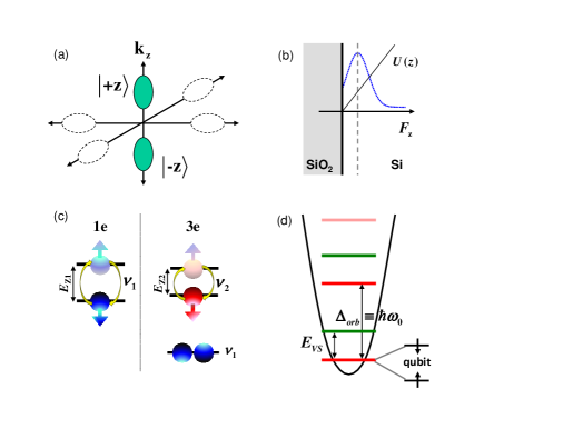
Figure 1: (a) The six valleys in Silicon. At an $(0,0,1)$ $\rm Si/SiO_{2}$ interface (a MOS structure) the low-energy subbands are formed by the $\pm\hat{z}$ valleys. (b) Confinement in $z$-direction at the $\rm Si/SiO_{2}$-interface and with an applied electric field $F_{z}$, forms the eigenvalley states $v_{1}$, $v_{2}$, split by a tunable valley splitting $E_{VS}\propto F_{z}$, see Eq. (29). Note, that the electron wave function $\varphi(z)$ and its derivative $\partial_{z}\varphi(z)$ may experience a discontinuity at the interface region, [see Sec. II.2 and Eq. (8)]. (c, d): For a small quantum dot the valley splitting is much smaller than the orbital splitting: $E_{VS}\ll\Delta_{\rm orb}\equiv\hbar\omega_{0}$, (typically Veldhorst et al. (2014); Yang et al. (2013); Jock et al. (2018), $E_{VS}=100-500\,\mu{\rm eV}$, $\Delta_{\rm orb}=2-8\,{\rm meV}$). (c) The one electron g-factor can be approximated by $g_{v_{1}}$, associated with the lower eigenvalley state $v_{1}$, while the three electron g-factor can be approximated by $g_{v_{2}}$, associated with the upper eigenvalley $v_{2}$. (d) Higher orbital states only introduce a small second-order effect (Sec. IV.2.2), such that one is actually measuring just the eigenvalley $g$-factors: $g_{1e}\simeq g_{v_{1}}$ and $g_{3e}\simeq g_{v_{2}}$.

This paper is a thorough study of the theoretical construction and its consequences that was suggested in our original short paper publication Veldhorst et al. (2015b). Results include general models of the valley splitting, valley-dependent SOC interactions, and valley-dependent anisotropic g-factors at a Si-heterostructure interface. In particular, (1) We obtain an interface modified effective mass approach where the electron spin and valley components are mixed at the heterostructure interface via a non-trivial boundary condition (BC), in the presence of a perpendicular electric field, Sec. II. This BC is equivalent to intervalley tunneling plus intervalley and intra-valley electron spin-flip processes, and reflects the interface $C_{\rm 2v}$ symmetry. The derived interface Hamiltonian is singular (in the heterostructure growth $z$-direction), which does not allow simple perturbation theory (PT) for the $g$-factor.

(2) We obtain from the BC a smooth interface 3D SOC tunneling Hamiltonian (Sec. III A) that allows PT for the $g$-factor renormalizations while maintaining the gauge invariance of the results. From the interface Hamiltonian we derive the electric field dependent valley splitting at the Si heterostructure, Sec. III B, for a general interface-confinement potential, allowing us to interpret the experiment of Ref. Yang et al., 2013.

(3) In the spin-valley mixing sector we obtain, in a translationally invariant form, the valley-diagonal Rashba and Dresselhaus effective 2D SOC Hamiltonians, as well as the off-diagonal in eigenvalleys Rashba and Dresselhaus SOCs, Sec. III C. The corresponding valley-dependent Rashba and Dresselhaus SOC constants for a linear $z$-confinement scale linearly with the electric field, $\propto F_{z}$, as does the valley splitting. The valley dependencies of the SOC constants suggest they may change sign when one switches between eigenvalleys, as a consequence of the dominance of the intervalley spin-flipping processes vs. the intravalley process.

(4) The valley-dependent $g$-factor tensor renormalizations for an in-plane magnetic field are derived in Sec. IV B from the smooth interface 3D SOC Hamiltonians, scaling as $\propto F_{z}^{2/3}$ for a linear $z$-confinement. For a perpendicular magnetic field, the relevant $g$-factor tensor components scale linearly with $F_{z}$, Sec. IV C, being proportional to the non-vanishing electric dipole matrix elements (scf. Refs. Yang et al. (2013); Gamble et al. (2013)).

(5) We show that the sign change of the SOC constants for different eigenvalleys leads to a corresponding sign change of the $g$-factor renormalization. In particular, for the in-plane magnetic field in a $[110]$-direction, we derive qualitatively and quantitatively that the $g$-factor renormalization is opposite in sign for an electron occupying different eigenvalley states, Fig. 1c, as it was observed in the experiment Veldhorst et al. (2015b), Sec. IV B.

(6) A prediction is made for the $g$-factor angular dependence on the in-plane magnetic field, as well as for an out-of-plane magnetic field in Sec. IV B, C, and D, that is in accordance with the $C_{\rm 2v}$ interface symmetry, which was confirmed in current experiments Jock et al. (2018); Tanttu et al. (2018). The $g$-factor angular dependence provides a single QD spin qubit with decoherence sweet spots with respect to the magnetic field direction.

(7) In Secs. IV B and C we consider second order corrections to the $g$-factor originating from the QD internal level structure, Fig. 1d, also including the effect of interface roughness Yang et al. (2013). For both the in-plane and perpendicular magnetic field configurations, these corrections (for a Si QD with strong lateral confinement) can be neglected: $\delta^{(2)}g\sim 10^{-6}$.

(8) Finally, in Sec. IV E, we compare our results to various current experiments Veldhorst et al. (2015b); Jock et al. (2018), providing in particular estimations for the ratio of the lower eigenvalley SOC constants, as well as for the difference of the SOC constants in both eigenvalleys subspaces with the account for the $g$-factor offsets for each eigenvalley. The dephasing mechanism introduced by the $g$-factor electric field dependence, is in a qualitative agreement with the experiment Veldhorst et al. (2015b). The results of Sec. IV can be seen as an experimental proposal to better understand the spin-valley structure at a Si interface. Section V contains the summary of results, and a discussion related to recent experiments with MOS QD structures Jock et al. (2018). More details of the derivations are presented in Appendices A, B, C.

II $\rm Si/SiO_{2}$ interface and boundary conditions

II.1 Valley and spin scattering at a $\rm Si/SiO_{2}$ heterostructure

We will consider a $\rm Si/SiO_{2}$ heterostructure grown along the $[001]$ ($\hat{z}$) direction with Si at $z>0$ under an applied electric field in the $\hat{z}$-direction, $(0,0,F_{z})$ corresponding to a linear potential $U_{z}(z)=|e|F_{z}z$. Due to a large conduction band offset to $\rm SiO_{2}$ ($\Delta_{\rm offset}\approx 3\,{\rm eV}$) we will approximate it with an infinite boundary, $U_{z}(z)=\infty,\,z<0$ (Fig. 1b).

A boundary condition at the heterostructure interface is a way to establish the interface scattering properties with respect to an incident waveOhkawa and Uemura (1977b); Sham and Nakayama (1979) with a wave vector $\bm{k}$ close to the band minima. At the Si heterostructure, due to $z$-confinement, there appear a mixingOhkawa (1978) between the two low-energy valley statesBoykin et al. (2004); Nestoklon et al. (2006); Jancu et al. (2005); Friesen et al. (2007) at $\bm{k}_{0}$ and $-\bm{k}_{0}$ (Fig. 1a and b), which implies intra-valley or inter-valley scattering. Generally, the scattering off the interface may lead not only to intervalley tunneling transitions ($\bm{k}_{0}\to-\bm{k}_{0}$), but also to a spin-flippingGolub and Ivchenko (2004); Boykin et al. (2004); Nestoklon et al. (2006); Jancu et al. (2005); Nestoklon et al. (2008); Rodina and Alekseev (2006), $\sigma\rightarrow-\sigma$ (see below).

Assuming the generalized envelope functions Kohn and Luttinger (1955), the total electron wave function is written in the single-band approximation as:

$$\Psi(\bm{r})=\left[\Phi_{\hat{z}}(\bm{r})\psi_{\bm{k}_{0}}(\bm{r})+\Phi_{-\hat{z}}(\bm{r})\psi_{-\bm{k}_{0}}(\bm{r})\right]$$ (4)

where the Bloch functions at the two band minima (at the $\Delta$ points) are $\psi_{\pm\bm{k}_{0}}(\bm{r})=e^{\pm i\bm{k}_{0}z}u_{\pm\bm{k}_{0}}(\bm{r})$, and $u_{\pm\bm{k}_{0}}(\bm{r})$ are the periodic amplitudes. The $\Phi_{\pm\hat{z}}(\bm{r})$ are spinor envelopes corresponding to the two valleys: $\Phi_{\hat{z}}(\bm{r})=[\Phi_{\hat{z},\uparrow}(\bm{r}),\Phi_{\hat{z},\downarrow}(\bm{r})]^{T}$ and $\Phi_{-\hat{z}}(\bm{r})=[\Phi_{-\hat{z},\uparrow}(\bm{r}),\Phi_{-\hat{z},\downarrow}(\bm{r})]^{T}$, with spin components $\sigma=\uparrow,\downarrow$; the envelopes $\Phi_{\pm\hat{z}}(\bm{r})=\Phi_{x,y}(x,y)\,\Phi_{\pm\hat{z}}(z)$ are separable in the absence of magnetic field.

In what follows, we consider an equivalent representation, in which the state is described as a four-component vector

$$\Phi(\bm{r})\equiv[\Phi_{\hat{z},\uparrow}(\bm{r}),\Phi_{\hat{z},\downarrow}(\bm{r}),\Phi_{-\hat{z},\uparrow}(\bm{r}),\Phi_{-\hat{z},\downarrow}(\bm{r})]^{T},$$ (5)

subject to boundary conditions and tunneling Hamiltonians.

II.2 Boundary conditions for $\rm Si/SiO_{2}$ heterostructure

The effective boundary condition at the $\rm Si/SiO_{2}$-interface will act on the four-component envelope $\Phi(\bm{r})$, Eq. (5), and it is derived from symmetry reasonings, for an infinitely high barrier (assuming a left interface at $z=z_{0}^{+}\equiv z_{0}+\varepsilon,\ \varepsilon\to+0$):

$$\left\{1+iR\,k_{z}-R\,\frac{2m_{l}}{\hbar^{2}}\,V_{\rm if}(\bm{k})\right\}\Phi(\bm{r})\mid_{z=z_{0}^{+}}\equiv{\cal B}\Phi(\bm{r})\mid_{z=z_{0}^{+}}=0.$$ (6)

Here $k_{j}\equiv-i\partial_{j}$ are quasi-momentum operators ($j=x,y,z$), ${\cal B}$ is a boundary operator, $R$ is a parameter of dimension of length, characterizing an abrupt interfaceVolkov and Pinsker (1979); Vasko (1979), and it is assumed that $R\ll l_{z},l_{D}$, where $l_{z},l_{D}$ are the QD confinement lengths along $z$-direction and in lateral directions. For $R=0$, Eq.(6) reduces to the standard BC, $\Phi(z)\mid_{z=z_{0}^{+}}=0$ (which is unphysical, see Appendix C.3). For $R\neq 0$ the BC leads to spin and valley mixing at the interface via the $4\times 4$ mixing matrix $V_{\rm if}(\bm{k})$ described in the next Sec. II.3.

The form of the BC, Eq.(6), can be understood through the general transfer matrix formalismAndo and Mori (1982), where hermiticity of the Hamiltonian across the interface is preserved using a transfer matrix $\hat{T}$ (has to be hermitean either) that relates the envelope function and its derivative normal to the interface on both sides of the interface (see also Ref.Tokatly et al. (2002); Rodina and Alekseev (2006) for a recent account). E.g., for the left interface for a single band and in the case of infinitely high barrier (spin-valley mixing is dropped for a while):

$$0=\left[\begin{array}[]{c}\Phi(z_{0}^{-})\\ \partial_{z}\Phi(z_{0}^{-})\end{array}\right]=\left(\begin{array}[]{cc}T_{11}&T_{12}\\ T_{21}&T_{22}\end{array}\right)\left[\begin{array}[]{c}\Phi(z_{0}^{+})\\ \partial_{z}\Phi(z_{0}^{+})\end{array}\right],$$ (7)

and a non-trivial solution of (7) implies the “resonant condition”Braginsky (1998) ${\rm det}\hat{T}=0$; so, $T_{12}\neq 0$. This means the relation

$$\Phi(z_{0}^{+})+iR\,k_{z}\Phi(z_{0}^{+})=0,$$ (8)

reproducing the first two terms in (6) with $R\equiv T_{12}/T_{11}$, and implying a discontinuity of the wave function and its derivative at the interface: $\Phi(z_{0}^{+})\neq 0$ and $k_{z}\Phi(z_{0}^{+})\neq 0$. In the last form, using the dimensional interface parameter $R$, the BC was first derived in Ref.Volkov and Pinsker, 1979, by requiring preservation of the hermiticity of the Hamiltonian in the half-space, $z>z_{0}$. Physically, this implies continuity of the envelope flux density Rodina and Alekseev (2006); Volkov and Pinsker (1979) (see also Appendix C.1). The parameter $R$, as well as the transfer matrix $\hat{T}$, is a characteristics of the interface boundary region; here, we will take it as a phenomenological parameter. An estimation, based on a two-band model (Appendix C.3) gives $|R|\approx 0.1-0.2\,{\rm nm}$ in the case of a $\rm Si/SiO_{2}$-interface.

If one drops the $k_{z}$-term in Eq. (6), then the BC is of the usual “non-resonant type” (in the sense of Ref.Braginsky, 1998), with $T_{12}=0$, and a transfer matrix obeys ${\rm det}\hat{T}_{\rm non-res}\neq 0$; this implies a continuous envelop function at the interface Rodina et al. (2003). Such BC have been suggested in Refs.Golub and Ivchenko, 2004; Nestoklon et al., 2006, 2008 for the case of a Si/SiGe interface, and their “non-resonant” character make them different from ours, Eq. (6).

In this paper we suggest that the surface contributions associated with the $k_{z}$-term can be important. In particular, the interface contribution to the $g$-factor change will be zero without this term. We also note, that for $R>0$, it is possible to consider the so called Tamm statesTamm (1932), (see also Refs.Volkov and Pinsker, 1979; Vasko, 1979; Rodina and Alekseev, 2006), leading to localization in the $\hat{z}$-direction even in the absence of electric field (to be considered elsewhere).

II.3 The $C_{\rm 2v}$ interface mixing matrix

The spin-valley mixing interface matrix $V_{\rm if}(\bm{k})$ that enters the BC (6), can be expressed by taking into account the $C_{\rm 2v}$ symmetry at the $\rm Si/SiO_{2}$ interface (see, e.g. Refs.Rashba and Sheka (1991); Golub and Ivchenko (2004); Nestoklon et al. (2006, 2008)^, ). The relevant $C_{\rm 2v}$-invariants are the Rashba and Dresselhaus $2\times 2$ forms: $H_{R}(\bm{k})=\sigma_{x}k_{y}-\sigma_{y}k_{x}$, $H_{D}(\bm{k})=\sigma_{x}k_{x}-\sigma_{y}k_{y}$. Indeed, for the $C_{\rm 2v}$-symmetry transformationsKiselev et al. (1998); Tokatly et al. (2002) one gets: (i) a $\pi_{z}$-rotation leading to $k_{x,y}\to-k_{x,y}$ and $\sigma_{x,y}\to-\sigma_{x,y}$, (ii) a reflection about the plane $(1,1,0)$, so that $k_{x}\leftrightarrow-k_{y}$ and $\sigma_{x}\leftrightarrow\sigma_{y}$, and (iii) a reflection about the plane $(1,\bar{1},0)$, with the $k_{x}\leftrightarrow k_{y}$ and $\sigma_{x}\leftrightarrow-\sigma_{y}$; it is then easy to see that $H_{R}(\bm{k})$ and $H_{D}(\bm{k})$ remain unchanged under these transformations. Thus, the $4\times 4$ spin-valley mixing matrix is parameterized as

$$V_{\rm if}(\bm{k})=\left(\begin{array}[]{cc}A(\bm{k})&V\bm{I}_{2}+B(\bm{k})\\ V^{*}\bm{I}_{2}+B^{+}(\bm{k})&A(\bm{k})\end{array}\right)$$ (11)

$$A(\bm{k})\equiv s_{D}\,H_{D}(\bm{k})+s_{R}\,H_{R}(\bm{k})$$ (12)

$$B(\bm{k})\equiv\chi_{D}\,H_{D}(\bm{k})+\chi_{R}\,H_{R}(\bm{k}),$$ (13)

where $s_{D,R}$ are real parameters, while the intervalley tunneling matrix elements $V=|V|e^{i\phi_{V}(z_{0})}$, and $\chi_{D,R}=|\chi_{D,R}|e^{i\phi_{D,R}(z_{0})}$ generally possess phases Nestoklon et al. (2006, 2008); Saraiva et al. (2009). For a general choice of the origin the phases depend linearly on $z_{0}$, $\phi_{V,D,R}(z_{0})=\phi_{V,D,R}-2ik_{0}z_{0}$, as it follows from the original valley Bloch functions in Eq. (4). The $2\times 2$ block-diagonal element $A(\bm{k})$ corresponds to intra-valley spin-flipping transitions. The Rashba-type term $s_{R}(\sigma_{x}k_{y}-\sigma_{y}k_{x})$ in the BC was previously derivedVasko (1979); Vasko and Kuznetsov (1998) for single-valley semiconductors. The constant $s_{R}$ has two contributions: $s_{R}=s^{\rm bulk}_{R}+s^{\rm if}_{R}$ and it can be shown that the bulk $g^{*}$-factor in Si can contribute to $s^{\rm bulk}_{R}$ (see, e.g. Refs. Vasko and Prima, 1981, 1981). However, in this paper we argue that interface contributions are dominating. In particular, at the interface, both Rashba and Dresselhaus contributions will be allowed.

The off-diagonal elements $V\bm{I}_{2}$ and $B(\bm{k})$ are related to an inter-valley tunneling (in momentum space). The non-spin-flipping term ($\sim V$) is responsible for the valley splittingOhkawa and Uemura (1977a, b); Sham and Nakayama (1979) (see also Refs.Saraiva et al. (2009); Culcer et al. (2010a); Friesen and Coppersmith (2010) for recent account). The inter-valley spin-flipping process will be described by the term $B(\bm{k})$. One of the main results of this paper is the observation that just this inter-valley spin-flipping process is dominating the description of the experimentally measured $g$-factor variations Veldhorst et al. (2015b).

II.4 Effective Hamiltonian for the $\rm Si/SiO_{2}$ heterostructure

The effective two-valley Hamiltonian acts on the four-component vector $[\Phi_{\hat{z},\uparrow}(\bm{r}),\Phi_{\hat{z},\downarrow}(\bm{r}),\Phi_{-\hat{z},\uparrow}(\bm{r}),\Phi_{-\hat{z},\downarrow}(\bm{r})]^{T}$ $\equiv\Phi(\bm{r})$, and includes a bulk Si (spin and valley degenerate) part

$${\cal H}_{0}=\left[\sum_{j=x,y,z}\frac{\hbar^{2}k_{j}^{2}}{2m_{j}}+U_{x,y}+U_{z}\right]\times\bm{I}_{4}$$ (14)

with the in-plane, $U_{x,y}$, and perpendicular to the interface, $U_{z}$, confinement electron potentials

$$U_{x,y}=\frac{m_{t}}{2}(\omega_{x}^{2}x^{2}+\omega_{y}^{2}y^{2})$$ (15)

$$U_{z}=\left\{\begin{array}[]{c}|e|(z-z_{0})F_{z},\ \ z>z_{0}\\ \infty,\ \ \ \ z<z_{0}\end{array}\right..$$ (18)

In what follows we consider a circular quantum dot Friesen and Coppersmith (2010), $\omega_{x}=\omega_{y}\equiv\omega_{0}$, and assume a much stronger confinement in the $\hat{z}$-direction: $l_{z}=(\hbar^{2}/2m_{l}|e|F_{z})^{1/3}\ll l_{D}=(\hbar/m_{t}\omega_{0})^{1/2}$, where $m_{l}$, $m_{t}$ are the longitudinal and transverse effective masses for $\Delta$-valley electrons, $|e|$ is the electron charge, and $F_{z}$ is the $z$-confinement electric field. For the parameters of the experiment Yang et al. (2013); Veldhorst et al. (2014, 2015b), for electric field $F_{z}\simeq 3\times 10^{7}\,{\rm V/m}$, $l_{z}\approx 1\,{\rm nm}$. The lateral QD size is $l_{D}\approx 7\,{\rm nm}$ for the 1e-case: $\Delta^{1e}_{\rm orb}\equiv\hbar\omega_{0}\simeq 8\,{\rm meV}$; for the 3e-case, $l_{D}\approx 14\,{\rm nm}$: $\Delta^{3e}_{\rm orb}\simeq 2\,{\rm meV}$ (since the “valence electron” in this case “sees” Coulomb repulsion, Figs. 1c and d). Here, $\Delta^{1e,3e}_{\rm orb}$, are the usual orbital splittings in the QD, Fig. 1d.

The BC (6) induces a $\delta$-functional Hamiltonian contribution, ${\cal H}_{\rm if}$ that mixes the spin and valley states:

$${\cal H}_{\rm if}=-\frac{\hbar^{2}}{2Rm_{l}}\delta(z-z_{0})\mp i\frac{\hbar^{2}}{2m_{l}}\delta(z-z_{0})k_{z}$$

$$\qquad\qquad\qquad{}+\delta(z-z_{0})V_{\rm if}(\bm{k}).$$ (19)

(To show Eq. (19), one needs to integrate the Schrödinger equation with ${\cal H}_{\rm if}$ at the vicinity of the boundary, $z=z_{0}$.) The $-$ ($+$) sign at the second term in Eq.(19) stands for left (right) interface, with the replacement $z_{0}=z_{\rm left}$ ($z_{0}=z_{\rm right}$) and, in general, the interface parameters at the two interfaces may be different, $R_{\rm left}\neq R_{\rm right}$). For a strong enough electric field the $z$-confinement (Fig. 1b) will keep electrons close to the left interface ($l_{z}\ll d_{\rm QW}\equiv z_{\rm right}-z_{\rm left}$), and we will neglect the influence of the right interface . We note that in the current experiment this is well fulfilled, since the $\rm{}^{28}Si$ QW thickness is $d_{\rm QW}\approx 300-800\,{\rm nm}$, while $l_{z}\approx 1\,{\rm nm}$ for $F_{z}\simeq 3\times 10^{7}\,{\rm V/m}$. Since $l_{z}\propto F_{z}^{-1/3}$, smaller electric fields are possible, providing the z-confinement energy splitting is much larger than the orbital splitting: $1.5\hbar^{2}/(m_{l}l^{2}_{z})\gg\hbar^{2}/(m_{t}l^{2}_{D})$; e.g., for $\Delta_{\rm orb}=1\,{\rm meV}$ one gets a typical field of $F_{z}\simeq 1.3\times 10^{6}\,{\rm V/m}$.

III Valley splitting, 2D(3D) effective Hamiltonians, and interface symmetry

III.1 The effective interface perturbation Hamiltonian

The interface contribution, Eq.(19), is essentially singular and cannot be used, in general, as a perturbation (except in a heuristic way). The effective interface perturbation Hamiltonian can be obtained by recasting the original problem of the Hamiltonian ${\cal H}_{0}$, Eq.(14), plus boundary conditions Eq.(6), to a standard BC, ${\cal B}\Phi\mid_{z=z_{0}^{+}}\equiv\tilde{\Phi}\mid_{z=z_{0}^{+}}=0$, and a transformed Hamiltonian. To this end we consider the 3rd term in the BC Eq.(6) as a perturbation (as $\langle k^{2}_{x}\rangle,\langle k^{2}_{y}\rangle\ll\langle k^{2}_{z}\rangle$) and replace the boundary operator ${\cal B}$ up to higher orders with a suitable unitary transform $\Gamma_{\rm BC}$ (Appendix A):

$$\tilde{\Phi}\mid_{z=z_{0}^{+}}\simeq\Gamma_{\rm BC}\Phi\mid_{z=z_{0}^{+}}=0$$ (20)

$$\tilde{{\cal H}}=\Gamma_{\rm BC}{\cal H}_{0}\Gamma^{\dagger}_{\rm BC}\simeq{\cal H}_{0}+\delta{\cal H},$$ (21)

with $\Gamma_{BC}=1+i[Rk_{z}+R^{2}\frac{2m_{l}}{\hbar^{2}}V_{\rm if}(\bm{k})k_{z}]$. Keeping only the leading contribution in (21) of order ${\cal O}(R^{2})$, one obtains:

$$\delta{\cal H}(z)\simeq R\partial_{z}U_{z}+R^{2}\frac{2m_{l}}{\hbar^{2}}V_{\rm if}(\bm{k})\partial_{z}U_{z}.$$ (22)

In the following we will neglect the first term in Eq.(22) which leads to a common energy shift only.

III.2 Approximate diagonalization of the interface matrix. Valley splitting

As suggested by the experiment Veldhorst et al. (2015b), the valley splitting matrix element is much stronger than the corresponding spin matrix elements val , $|V|\gg\{|\chi_{R,D}|,s_{R,D}\}\langle k_{x,y}\rangle$, and the interface spin-valley matrix is represented as $V_{\rm if}(\bm{k})=V_{\rm if,val}+{\cal O}(1/|V|)$ with

$$V_{\rm if,val}=\left(\begin{array}[]{cc}0&V\bm{I}_{2}\\ V^{*}\bm{I}_{2}&0\end{array}\right).$$ (23)

Thus, one diagonalizes the interface Hamiltonian, Eq. (22), to leading order via the unitary transform (we choose below $z_{0}=0$ for convenience)

$$U_{\rm v}=\frac{1}{\sqrt{2}}\left(\begin{array}[]{cc}\bm{I}_{2}&-e^{i\phi_{V}}\bm{I}_{2}\\ e^{-i\phi_{V}}\bm{I}_{2}&\bm{I}_{2}\end{array}\right),$$ (24)

leading to spin-independent valley-splitting Hamiltonian

$$\delta{\cal H}_{\rm if,val}=\frac{2m_{l}}{\hbar^{2}}R^{2}\,V^{\rm d}_{\rm if,val}\,\partial_{z}U_{z},$$ (25)

with $V^{\rm d}_{\rm if,val}={\rm diag}(|V|\bm{I}_{2},-|V|\bm{I}_{2})$. The corresponding spin-degenerate eigenstates are denoted as $|v^{\rm d}_{2,\sigma}\rangle=[C^{T}_{\sigma},0,0]^{T}$ and $|v^{\rm d}_{1,\sigma}\rangle=[0,0,C^{T}_{\sigma}]^{T}$ for the upper and lower eigenvalley states, respectively; $C_{\sigma}$ is a spinor, corresponding to the two spin projections along an applied $\bm{B}$-field. Turning back to the original $\pm\hat{z}$-valley basis, the eigenstates of the leading-order Hamiltonian ${\cal H}_{0}+\delta{\cal H}_{\rm if,val}$ will be written as

$$|\bar{v}_{i;\sigma}\rangle=\frac{1}{\sqrt{2}}\left[\begin{array}[]{c}C_{\sigma}\\ \mp e^{-i\phi_{V}}C_{\sigma}\end{array}\right]\,\phi_{0}(x,y)\,\tilde{\varphi}_{0}(z),\ \ i=1,2$$ (28)

where $\phi_{0}(x,y)\,\tilde{\varphi}_{0}(z)$ is an eigenstate of ${\cal H}_{0}$, Eq.(14), with BC, $\tilde{\varphi}_{0}(0^{+})=0$, in the lowest $z$-subband. The upper/lower eigenvalley energies are $E_{2,1}=\langle\bar{v}_{2,1}|\delta{\cal H}_{\rm if,val}|\bar{v}_{2,1}\rangle=\pm\frac{|V|2m_{l}R^{2}}{\hbar^{2}}\,\langle\tilde{\varphi}_{0}(z)|\partial_{z}U_{z}|\tilde{\varphi}_{0}(z)\rangle\equiv\pm\frac{|V|2m_{l}R^{2}}{\hbar^{2}}\,\langle\partial_{z}U_{z}\rangle$ and the valley splitting reads:

$$E_{\rm VS}=2|V|R^{2}\frac{2m_{l}}{\hbar^{2}}\,\langle\tilde{\varphi}_{0}(z)|\partial_{z}U_{z}|\tilde{\varphi}_{0}(z)\rangle.$$ (29)

By observing the general integral relation (Appendix B.4)

$$\langle\tilde{\varphi}(z)|\partial_{z}U_{z}|\tilde{\varphi}(z)\rangle\equiv\int_{0}^{\infty}\,dz\tilde{\varphi}^{*}(z)\partial_{z}U_{z}\tilde{\varphi}(z)=\frac{\hbar^{2}}{2m_{l}}\,|\tilde{\varphi}^{\prime}(0)|^{2}$$ (30)

[It holds for any eigenstate of the Hamiltonian (14) with a smooth (at $z>0$) $z$-confinement potential $U_{z}$ and zero BC, $\tilde{\varphi}(0)=0$], one can recast the valley splitting to the form

$$E_{\rm VS}=2|V|R^{2}\,|\tilde{\varphi}_{0}^{\prime}(0)|^{2}.$$ (31)

Alternatively, the valley splitting can be derived in a different (heuristic) way, using the singular Hamiltonian, Eq.(19). In this case, one would consider the first two terms in Eq.(19) as a leading order boundary condition, recasting them to the Volkov-Pinsker formVolkov and Pinsker (1979)

$$[1+R\partial_{z}]\varphi_{0}(0)=0,$$ (32)

[scf. Eq.(6)]. Since R is small, one essentially has the BC $\varphi_{0}(R)=0$ which corresponds to $z$-shifting the origin by R. With $\varphi_{0}(z)$ being the eigenstate of the Hamiltonian (14) ${\cal H}_{0}$ with the above BC (32) one considers the “perturbation” $\delta(z)\,V^{\rm d}_{\rm if,val}$ from Eq.(19), with the diagonal part of the interface matrix. This gives the valley splitting

$$E_{\rm VS}=2|V||\varphi_{0}(0)|^{2}\simeq 2|V|R^{2}|\varphi_{0}^{\prime}(0)|^{2}\simeq 2|V|R^{2}|\tilde{\varphi}_{0}^{\prime}(0)|^{2},$$ (33)

where we have used Eq. (32), and that $\tilde{\varphi}_{0}^{\prime}(0)\simeq{\varphi}_{0}^{\prime}(0)$ up to higher orders in R. The result, Eq.(33), for the valley splitting coincides with Eqs. (29) and (31), obtained via the effective Hamiltonian Eq.(22).

Notice that for ${\cal H}_{0}$, Eq.(14), with the linear $z$-confinement potential $U_{z}=|e|F_{z}z$ (the “triangular” potential) one has the lowest energy subband function: $\tilde{\varphi}_{0}(z)=N_{1}\,l_{z}^{-1/2}\,{\rm Ai}(l_{z}^{-1}z-\tilde{E}_{1})$ with a normalization $N_{1}\simeq 1.4261$, and $-\tilde{E}_{1}=-2.3381$ being the first zero of the Ai function. The $z$-average is $\langle z\rangle\simeq 1.5587\,l_{z}=1.5587\,(\hbar^{2}/2m_{l}|e|F_{z})^{1/3}$, see Eq.(14). For the valley splitting one gets then from Eq.(29):

$$E_{\rm VS}=2|V|R^{2}\,\frac{2m_{l}|e|F_{z}}{\hbar^{2}}=2|V|R^{2}l_{z}^{-3}.$$ (34)

Thus, the general relation Eq. (31) we have proven, (Appendix B.4) is fulfilled here from the relation $\frac{d\tilde{\varphi}_{0}(z)}{dz}=N_{1}\,l_{z}^{-3/2}\,{\rm Ai}^{\prime}(l_{z}^{-1}z-\tilde{E}_{1})$ and by noticing that $N_{1}{\rm Ai}^{\prime}(-\tilde{E}_{1})=1$.

For the second (heuristic) approach, with the “shifted BC” Eq.(32), the eigenstates of the Hamiltonian, Eq.(14) will be just the shifted functions, with the lowest subband being:

$$\varphi_{0}(z)=N_{1}\,l_{z}^{-1/2}\,{\rm Ai}(l_{z}^{-1}(z-R)-\tilde{E}_{1}),$$ (35)

and $|\varphi_{0}(0)|=R|\varphi^{\prime}_{0}(0)|\simeq R|\tilde{\varphi}^{\prime}_{0}(0)|\neq 0$, as implied by Eq.(31) and the Volkov-Pinsker BC, Eq.(32).

The linear dependence on $F_{z}$, Eq. (34), is confirmed experimentallyYang et al. (2013); Veldhorst et al. (2014). Using the estimation $R\approx 0.1\,{\rm nm}$ (Appendix C.3) and the experimental slope Yang et al. (2013) $\frac{\Delta E_{\rm VS}}{\Delta F_{z}}=1.32\,\,{\rm e\,{\AA}}$ one gets a valley-splitting parameter $|V|\approx 2640\,\,{\rm meV}\,{\rm{\AA}}$ compatible with the effective mass and tight-binding calculations Friesen et al. (2007); Nestoklon et al. (2008) (extrapolated to the $\rm Si/SiO_{2}$ caseV-s ).

Eq. (34) corresponds to a valley splitting with linear $F_{z}$-dependence and no offset, applicable for relatively large electric fields, $F_{z}\gtrsim 3\times 10^{7}{\rm V/m}$, when $z$-confinement is much stronger than lateral confinement. (Notice, however, that for larger QDs our results are applicable at lower electric fields as well). On the other hand, the measurements of the valley splitting in our previous work Yang et al. (2013); Veldhorst et al. (2014) suggest that such offset could be possible. For example, a possible non-linear dependence at small electric field suggested by tight-binding calculations Boykin et al. (2004); Nestoklon et al. (2008) could lead to an effective offset.

Here we propose a phenomenological approach that allows to describe the experimentally observed valley splitting offsetYang et al. (2013); Veldhorst et al. (2014) resulting from an interface localized interaction. Using the general results, Eqs. (29)-(33), one considers a confinement potential of the form $U_{z}=\frac{1}{2}m_{l}\omega_{z}^{2}z^{2}+|e|zF_{z}$, which provides a non-zero valley splitting at $F_{z}=0$, with a confinement length factor, $l_{\rm osc}^{-3}\equiv|\tilde{\varphi}_{0}^{\prime}(0)|^{2}=\frac{8}{\sqrt{\pi}}\left(\frac{m_{l}\omega_{z}}{\hbar}\right)^{3/2}$. In the opposite limit of large $F_{z}$, the zero-field confinement can be considered as a perturbation to the linear potential, leading asymptotically to the behavior: $E^{\rm asympt}_{\rm VS}\simeq 2|V|R^{2}\,\frac{2m_{l}}{\hbar^{2}}(|e|F_{z}+m_{l}\omega_{z}^{2}\langle z\rangle)$, which can be interpreted as a positive offset. To obtain a negative offset, one needs to replace the interface-localized confinement with a repulsion $z$-potential.

III.3 Approximate diagonalization of the interface matrix: The 2D Spin-Orbit Dresselhaus and Rashba couplings and effective 2D (3D) Hamiltonians

The effective spin-orbit Hamiltonians (of Rashba and Dresselhaus type) are obtained similarly to the $E_{VS}$ calculation. For this end, we apply now the unitary transformation $U_{\rm v}$, Eq. (24), to the full interface matrix, $V^{\rm U}_{\rm if}(\bm{k})=U_{\rm v}^{+}V_{\rm if}(\bm{k})U_{\rm v}$ and obtain the form:

$$V^{\rm U}_{\rm if}(\bm{k})=\left(\!\!\begin{array}[]{cc}|V|\bm{I}_{2}&0\\ 0&-|V|\bm{I}_{2}\end{array}\!\!\right)+\left(\!\!\begin{array}[]{cc}A+\frac{1}{2}B_{\rm diag}&\frac{1}{2}B_{\rm off}\\ {\rm h.c.}&A-\frac{1}{2}B_{\rm diag}\end{array}\!\!\right)\quad\ \$$ (40)

$$\qquad\quad\equiv V^{\rm d}_{\rm if,val}+V^{\rm s-v}_{\rm if}(\bm{k}),$$

with

$$B_{\rm diag}\equiv B(\bm{k})e^{-i\phi_{V}(z_{0})}+B^{+}(\bm{k})e^{i\phi_{V}(z_{0})},$$ (41)

$$B_{\rm off}\equiv B(\bm{k})-B^{+}(\bm{k})e^{2i\phi_{V}(z_{0})},$$ (42)

obtained via Eq.(13), with $\phi_{V}(z_{0})=\phi_{V}-2ik_{0}z_{0}$.

The spin-valley mixing part in (40), $V^{\rm s-v}_{\rm if}(\bm{k})$, consists of the (eigen)valley block-diagonal and off-diagonal parts and constitutes the spin-orbit effective coupling at the interface, derived from Eq. (22):

$$\delta{\cal H}_{\rm s-v}=R^{2}\frac{2m_{l}}{\hbar^{2}}\,V^{\rm s-v}_{\rm if}(\bm{k})\,\partial_{z}U_{z}$$

$$\qquad\quad{}=V^{\rm s-v}_{\rm if}(\bm{k})\,R^{2}|\varphi_{0}^{\prime}(0)|^{2}\frac{\partial_{z}U_{z}}{\langle\partial_{z}U_{z}\rangle},$$ (43)

with matrix elements between the eigenvalley states $v_{1}$, $v_{2}$, that are proportional to the Rashba and Dresselhaus invariant forms, $H_{R}(\bm{k})$, $H_{D}(\bm{k})$. The spin-valley mixing Hamiltonian $\delta{\cal H}_{\rm s-v}$, Eq. (43), then reads:

$$\delta{\cal H}_{\rm s-v}=$$

$${}=\left(\!\!\!\!\begin{array}[]{cc}\alpha_{R;v_{2}}H_{R}+\beta_{D;v_{2}}H_{D},&\!\!\alpha_{R;21}H_{R}+\beta_{D;21}H_{D}\\ \alpha_{R;21}^{*}H_{R}+\beta_{D;21}^{*}H_{D},&\!\!\alpha_{R;v_{1}}H_{R}+\beta_{D;v_{1}}H_{D}\end{array}\!\!\!\!\right)\!\!\frac{\partial_{z}U_{z}}{\langle\partial_{z}U_{z}\rangle},\ \ \ \$$ (46)

where $\alpha_{R;v_{i}}$, $\beta_{D;v_{i}}$, and $\alpha_{R;21}$, $\beta_{D;21}$ are the diagonal and off-diagonal (valley dependent) Rashba and Dresselhaus coupling constants, related to the effective SOC interactions considered below. We derive the SOC constants, taking into account the phases of $\chi_{R}=|\chi_{R}|e^{i\phi_{R}(z_{0})}$, $\chi_{D}=|\chi_{D}|e^{i\phi_{D}(z_{0})}$ in a translationally invariant form tra . For the diagonal constants one obtains:

$$\alpha_{R;v_{i}}=\left[s_{R}\mp|\chi_{R}|\cos(\phi_{R}-\phi_{V})\right]\,R^{2}|\varphi_{0}^{\prime}(0)|^{2}$$ (47)

$$\beta_{D;v_{i}}=\left[s_{D}\mp|\chi_{D}|\cos(\phi_{D}-\phi_{V})\right]\,R^{2}|\varphi_{0}^{\prime}(0)|^{2}$$ (48)

$$i=1,2$$

with $-$ ($+$) corresponding to the lower eigenvalley $v_{1}$ (upper eigenvalley $v_{2}$) respectively; this is similar to the relevant strong field limit results of Ref.Nestoklon et al., 2008. The off-diagonal Rashba and Dresselhaus coupling constants are, correspondingly:

$$\alpha_{R;21}=ie^{i\phi_{V}}|\chi_{R}|\sin(\phi_{R}-\phi_{V})\,R^{2}|\varphi_{0}^{\prime}(0)|^{2}$$ (49)

$$\beta_{D;21}=ie^{i\phi_{V}}|\chi_{D}|\sin(\phi_{D}-\phi_{V})\,R^{2}|\varphi_{0}^{\prime}(0)|^{2}.$$ (50)

Notice that for a linear $z$-confinement, Eq. (18), the SOC constants scale linearly with the applied electric field $F_{z}$. The off-diagonal elements $\alpha_{R;21}$, $\beta_{D;21}$ could be, generally, of the same order as the diagonal one, $\alpha_{R;v_{i}}$, $\beta_{D;v_{i}}$, depending on the phases, $\phi_{V}$, $\phi_{R}$, $\phi_{D}$, and assuming $|\chi_{R,D}|\gtrsim s_{R,D}$. These parameters, including the phases, enter in the observable SOC constants in certain combinations, relating the diagonal to off-diagonal (in valley) SOC constants, Eqs. (47)-(50). Eq. (46) and Eqs. (47)-(50) describe the 3D spin-valley mixing at the interface. These equations are one of the main results of this paper, together with the $g$-factor derivation in the next chapter, which will be based on them as well.

A 2D version can be obtained by integration over the $z$-direction. The effective 2D Hamiltonian with Rashba and Dresselhaus contributions in each eigenvalley subspace is given by the corresponding block-diagonal parts in Eq. (46):

$${\cal H}^{\rm 2D}_{v_{i}}=\alpha_{R;v_{i}}\,H_{R}(\bm{k})+\beta_{D;v_{i}}\,H_{D}(\bm{k}),\ \ i=1,2,$$ (51)

with the 2D spin-orbit couplings given by Eqs. (47) and (48). Similarly, the 2D Hamiltonian that describes the off-diagonal transitions between the eigenvalley subspaces $v_{1},v_{2}$ can be written in the form

$${\cal H}^{\rm 2D}_{v_{2},v_{1}}=\alpha_{R;21}H_{R}(\bm{k})+\beta_{D;21}H_{D}(\bm{k}),$$ (52)

with the 2D spin-orbit couplings given by Eqs. (49) and (50).

As seen from Eqs. (47)-(50), all the above spin-orbit constants depend on the common matrix elements constants, $V$, $s_{R}$, $s_{D}$, $\chi_{R}$, $\chi_{D}$, that parameterize the spin-valley mixing boundary condition, Eq. (6). We note, that the 2D spin-orbit Rashba and Dresselhaus constants, $\alpha_{R;v_{i}}$, $\beta_{D;v_{i}}$, may change sign when one switches between the eigenvalley subspaces $v_{1}\to v_{2}$:

$$\alpha_{R;v_{1}}\simeq-\alpha_{R;v_{2}}\ {\rm and}\ \ \beta_{D;v_{1}}\simeq-\beta_{D;v_{2}}$$ (53)

if the inter-valley contributions, $\chi_{R}$, $\chi_{D}$ dominate the intravalley ones, $s_{R}$, $s_{D}$; Eq. (53) is exact for $s_{R},s_{D}=0$. As shown in the next Sec. IV, this is in qualitative agreement with the experiment Veldhorst et al. (2015b), where measurement of the $g$-factor were performed for an in-plane magnetic field.

Finally, we mention that one can derive the 2D Hamiltonian Eq. (46) without recasting the BC to a smooth perturbation Hamiltonian [as it was done in Eqs.(21) and (22)]. As in the valley splitting derivation in Eq.(33), one just refers to the leading order BC, Eq.(32), and uses (heuristically) the singular “perturbation” $\delta(z)\,V^{\rm U}_{\rm if}(\bm{k})$ with the full interface matrix, Eq.(40). The effective interface Hamiltonian, Eq. (22), is necessary, however, for the derivation of the $g$-factor where the heuristic approach does not work.

IV Electron $g$-factor at the interface

IV.1 Derivation of the $g$-factor corrections

We will consider for each eigenvalley the Hamiltonians, Eqs.(14) and (25), ${\widetilde{\cal H}}_{0}={\cal H}_{0}+\delta{\cal H}_{\rm if,val}$ as the zeroth-order term, and the spin-valley mixing term $\delta{\cal H}_{\rm s-v}$, Eqs. (43) and (46), as a perturbation. Since the valley splitting is large, one can neglect the block-off-diagonal part in $\delta{\cal H}_{\rm s-v}$ as it contributes to the energy renormalization of the subspaces $v_{1}$, $v_{2}$, only in second order of PT, and is suppressed as $\sim|\chi_{D,R}\langle k_{x,y}\rangle|/E_{\rm VS}$. The block-diagonal parts of $\delta{\cal H}_{\rm s-v}$ are of the form

$${\cal H}_{v_{i}}^{\rm 3D}=\left[\alpha_{R;v_{i}}\,H_{R}(\bm{k})+\beta_{D;v_{i}}\,H_{D}(\bm{k})\right]\,\frac{\partial_{z}U_{z}}{\langle\partial_{z}U_{z}\rangle},\ \ i=1,2.$$ (54)

One can note that these Hamiltonians are in one-to-one correspondence, via Eqs. (21)-(22), to the BCs in each eigenvalley subspace sin :

$$\left\{1+iRk_{z}-R\frac{2m_{l}}{\hbar^{2}}\left[\mp|V|+V_{v_{i}}(\bm{k})\right]\right\}\Phi_{v_{i}}(\bm{r})\mid_{z=z_{0}^{+}}=0,$$ (55)

with the spin-mixing matrix $V_{v_{i}}(\bm{k})\equiv A\mp\frac{1}{2}\,B_{\rm diag}$ defined in Eqs. (12), (13), and (41), and acting on the corresponding eigenvalley spinors, $\Phi_{v_{i}},\,i=1,2$. Eq. (54) may contribute to first order of PT to the g-factor in each eigenvalley subspace.

For a magnetic field a direct Zeeman term is added to the zeroth-order Hamiltonian ${\widetilde{\cal H}}_{0}$:

$${\cal H}_{\rm Z}=g^{*}\mu_{B}\frac{1}{2}\bm{\sigma}\bm{B}$$ (56)

where $\mu_{\rm B}$ is the Bohr magneton; the bulk Si effective $g^{*}$-factor Wilson and Feher (1960); Roth (1960); Liu (1962), is $g^{*}_{\rm Si}\simeq 1.9983$ (at the interface).

The perturbation due to external magnetic field will arise via the replacement Kohn and Luttinger (1955) $k_{j}\to k_{j}+\frac{|e|}{\hbar}A_{j}(\bm{r})$ [$\bm{A}(\bm{r})$ is the vector-potential], both in ${\cal H}_{0}$ and in the interface Hamiltonian $\delta{\cal H}_{\rm s-v}$ or, equivalently, in the respective BCs, Eqs. (6), (19), and (55), which makes the problem gauge invariant [For a gauge-invariant BC without spin and valleys, see Appendix C.1; for a discussion of gauge-invariance see Appendix C.2]. Introducing the magnetic length, $l_{B}=(\hbar/|e|B)^{1/2}$, we require a stronger $z$-confinement, $l_{z}\ll l_{B}$, which is fulfilled in the experiment for $B=1.4\,{\rm T}$, as $l_{B}(1.4\,{\rm T})\simeq 22\,{\rm nm}$.

IV.2 g-factor for in-plane magnetic field, $\bm{B}_{\parallel}$

IV.2.1 $\delta g_{\parallel}$ to 1st-order PT

For an in-plane magnetic field one chooses the gauge $\bm{A}_{\|}(\bm{r})=(B_{y}z,-B_{x}z,0)$. In what follows, we neglect small corrections originating from the bulk Hamiltonian ${\cal H}_{0}$, Eq. (14). The perturbation to Eq. (54), $\delta_{B}{\cal H}_{v_{i}}^{\rm 3D}$, due to non-zero magnetic field $\bm{B}_{\parallel}$, contributes to the g-factor interface contribution, $\delta g^{v_{i}}_{\parallel}$, to first order. Averaging Eq. (54) over the states $|\bar{v}_{i}\rangle\equiv|v_{i}\rangle\otimes|\phi_{v_{i}}(\bm{r})\rangle$ [that includes the envelope wave function of the confined electron $|\phi_{v_{i}}(\bm{r})\rangle\equiv\phi_{0}^{v_{i}}(x,y)\varphi_{0}(z)$, see below], for each eigenvalley gives

$$\langle\bar{v}_{i}|\delta_{B}{\cal H}_{v_{i}}^{\rm 3D}|\bar{v}_{i}\rangle=a[U_{z}]\ \mu_{B}\Big{[}\alpha_{R;v_{i}}(\sigma_{x}B_{x}+\sigma_{y}B_{y})\Big{.}$$

$$\qquad\qquad\qquad\ \ \Big{.}{}-\beta_{D;v_{i}}(\sigma_{x}B_{y}+\sigma_{y}B_{x})\Big{]},\ \ i=1,2$$ (57)

$$\qquad a[U_{z}]\equiv-\frac{|e|}{\hbar\mu_{B}}\frac{\langle z\partial_{z}U_{z}\rangle}{\langle\partial_{z}U_{z}\rangle},\ \ \ a[U_{z}]\sim 10^{-3},$$ (58)

with the constant $a[U_{z}]$ being a weakly-dependent functional of the z-confinement potential $U_{z}$. For a constant electric field $a[U_{z}]$ is replaced by $-\frac{|e|\langle z\rangle}{\hbar\mu_{B}}$. The total Zeeman energy can be written via the g-factor tensor:

$${\cal H}^{\rm tot}_{\rm Z,v_{i}}=\sum_{\alpha,\beta}\frac{1}{2}\mu_{B}\left(g_{0}\delta_{\alpha\beta}+\delta g^{v_{i}}_{\alpha\beta}\right)\sigma_{\alpha}B_{\beta},$$ (59)

where $g_{0}=g^{*}_{\rm Si}$ is the bulk value in Si, and

$$\delta g_{xx}^{v_{i}}=\delta g_{yy}^{v_{i}}=-a[U_{z}]\ \alpha_{R;v_{i}}$$ (60)

$$\delta g_{xy}^{v_{i}}=\delta g_{yx}^{v_{i}}=+a[U_{z}]\ \beta_{D;v_{i}}\,.$$ (61)

The Zeeman splitting is expressed as $\Delta E\equiv\mu_{B}g_{\parallel}(\varphi)B_{\parallel}$, $B_{\parallel}=\sqrt{B_{x}^{2}+B_{y}^{2}}$, and $B_{x}=B_{\parallel}\cos\varphi$, $B_{y}=B_{\parallel}\sin\varphi$, being the magnetic field components along the Si crystal axes. By diagonalization of the Hamiltonian (59) for each valley subspace, one obtains the total g-factor $g_{\|}^{v_{i}}(\varphi,F_{z})$,

$$g_{\parallel}^{v_{i}}(\varphi,F_{z})=\Big{(}g_{0}^{2}+2a[U_{z}]\,g_{0}\,[\alpha_{R;v_{i}}-\beta_{D;v_{i}}\sin 2\varphi]+\Big{.}\qquad\qquad\quad$$

$$\qquad\quad\Big{.}{}+a[U_{z}]^{2}\,\,[\alpha^{2}_{R;v_{i}}+\beta^{2}_{D;v_{i}}-2\alpha_{R;v_{i}}\beta_{D;v_{i}}\sin 2\varphi]\Big{)}^{1/2}\!\!\!\!,$$ (62)

that includes the interface contribution $\delta g_{\parallel}^{v_{i}}$: $g_{\|}^{v_{i}}\equiv g_{0}+\delta g_{\parallel}^{v_{i}}$. The $F_{z}$ dependence in Eq. (62) is implicit via the SOC constants and $z$-averages, Eqs. (47),(48), (30), and (58). To first order in $a[U_{z}]$ it gives the g-factor interface variation as a function of the in-plane magnetic field directionRuskov (2016); Tahan (2015), $\varphi$ (Fig. 2):

$$\delta g_{\parallel}^{v_{i}}(\varphi,F_{z})\simeq\delta^{(1)}g_{v_{i}}=-\frac{|e|}{\hbar\mu_{B}}\frac{\langle z\partial_{z}U_{z}\rangle}{\langle\partial_{z}U_{z}\rangle}\,\left(\alpha_{R;v_{i}}-\beta_{D;v_{i}}\sin 2\varphi\right).$$ (63)

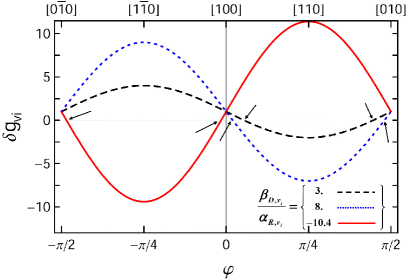
Figure 2: Angular dependence of the $g$-factor correction $\delta g_{\parallel}^{v_{i}}(\varphi,F_{z})$, Eq. (63) at different ratios of the spin-orbit parameters: $\beta_{D;v_{i}}/\alpha_{R;v_{i}}=\{3.0,\,8.0,\,-10.4\}$ (dashed black, dotted blue, and red curves, respectively); $\delta g_{\parallel}^{v_{i}}$ is in units of $\frac{e}{\hbar\mu_{B}}|\alpha_{R;v_{i}}|$. For $\bm{B}_{\parallel}$ at angles (shown with arrows) $\varphi_{v_{i}}$, Eq. (65), measured from the $[1,0,0]$ crystal direction, the QD spin-qubit is immune to the charge noise on $F_{z}$, since the g-factor variation due to electric field noise goes to zero together with $\delta g_{\parallel}^{v_{i}}(F_{z})$, see Eqs. (64), (66), and (84).

The angular dependence on the direction of the in-plane magnetic field suggests that there could be valley-dependent “sweet spot directions” $\varphi_{v_{i}}$ where the $g$-factor variation with the electric field is zero. Since from Eq. (63),

$$\frac{\partial[\delta g_{\parallel}^{v_{i}}(\varphi,F_{z})]}{\partial F_{z}}=\frac{\partial\ln\langle z\,\partial_{z}U_{z}\rangle}{\partial F_{z}}\ \delta g_{\parallel}^{v_{i}}(\varphi,F_{z})$$ (64)

the $g$-factor noise variation gets to zero together with $\delta g_{\parallel}^{v_{i}}(F_{z})$. For a given eigenvalley $v_{i}$ the choice of the angle $\varphi_{v_{i}}$ will depend on the size and sign of the Rashba and Dresselhaus 2D spin-orbit constants, $\alpha_{R;v_{i}}$, $\beta_{D;v_{i}}$. The 1st-order PT $g$-factor correction, Eq. (63), can be put to zero when $\sin(2\varphi)=\alpha_{R;v_{i}}/\beta_{D;v_{i}}$. Thus, the optimal angles are expressed as (Fig. 2):

$$\varphi_{v_{i}}=\frac{1}{2}\,\arcsin\left(\frac{\alpha_{R;v_{i}}}{\beta_{D;v_{i}}}\right)\simeq\frac{\alpha_{R;v_{i}}}{2\beta_{D;v_{i}}}+k\frac{\pi}{2},\ \ k=0,\pm 1,\pm 2,\dots,$$ (65)

where the inequality $|\alpha_{R;v_{i}}|\ll|\beta_{D;v_{i}}|$ is assumed from tight binding calculations Nestoklon et al. (2008), . The sweet spot angles are generally different for the two eigenvalley states $v_{i}$. At these angles the spin qubit is immune to the charge noise (via the electric field $F_{z}$, see Sec. IV.5.3). However, at the same sweet spot angles the qubit frequency cannot be manipulated as well. (From a qubit perspective, there should be a trade off, where one can keep the possibility to manipulate the qubit reasonably fast, and simultaneously minimize the noise). There are weak second order PT effects, to be considered in the next section. It is interesting to note that for a zero Dresselhaus contribution the $g$-factor variation $\delta g_{\parallel}^{v_{i}}$ becomes angle-independent.

For a linear $z$-confinement one can rewrite Eq. (63) as

$$\delta g_{\parallel}^{v_{i}}(\varphi,F_{z})\equiv A_{v_{i}}(\varphi)F_{z}^{2/3},$$ (66)

since the SOC constants $\alpha_{R;v_{i}},\beta_{D;v_{i}}\propto F_{z}$, and the average of the $z$-motion in the lowest subband is $\langle z\rangle\simeq 1.5587\,(\hbar^{2}/2m_{l}|e|F_{z})^{1/3}$, see Eq.(14). In the experiment Veldhorst et al. (2015b), where the magnetic field is parallel to the $[110]$-direction (i.e. $\varphi=\pi/4$), one gets from Eq. (63):

$$\delta g_{\parallel}^{v_{i}}(\pi/4,F_{z})=-\frac{(\alpha_{R;v_{i}}-\beta_{D;v_{i}})|e|}{\hbar\mu_{\rm B}}\langle z\rangle$$ (67)

[for a discussion of the gauge-invariance of this result, see Appendix C.2]. The $g$-factor scales as $F_{z}^{2/3}$, which is close to a linear scaling over the range ($\sim 6\%$) of the experimentally applied electric fields, see Fig. 3b.

Since the in-plane $g$-factor correction, $\delta g_{\parallel}^{v_{i}}$, is proportional to $\alpha_{R;v_{i}}$, $\beta_{D;v_{i}}$ it is clear that for the two eigenvalley subspaces it may change sign along with the sign change of $\alpha_{R;v_{i}}$, $\beta_{D;v_{i}}$, Eq. (53). E.g., for the intra-valley spin-flip parameters being exactly zero, $s_{R},s_{D}=0$, the $g$-factor correction will be exactly opposite

$$\delta g_{\parallel}^{v_{1}}=-\delta g_{\parallel}^{v_{2}}.$$ (68)

Relatively smaller corrections due to non-zero intra-valley spin flipping, $s_{R},s_{D}\neq 0$ will generally violate Eq. (68), leaving the $g$-factor corrections opposite in sign, but with different absolute value, $|\delta g_{\parallel}^{v_{1}}|\neq|\delta g_{\parallel}^{v_{2}}|$, which is observed in the current experimentVeldhorst et al. (2015b), see Fig. 3. Tight-binding calculationsNestoklon et al. (2008) were performed for the case of a Si/SiGe interface, with the result that $|\chi_{D}|\gg|s_{D}|$, $|\chi_{R}|\gg|s_{R}|$, while $|\chi_{R}|\sim|s_{D}|$, supporting the case of Eqs. (53) and (68). For comparison of the results Eqs. (63)-(67) with the experiment, see Sec. IV.5.

IV.2.2 $\delta g_{\parallel}$ to 2nd-order PT

Since at certain angles of the in-plane magnetic field, Eq. (65), the g-factor 1st-order correction can be zeroed, one needs to calculate also higher order effects, which arise due to QD’s energy level structure.

We consider a small quantum dot (QD) in MOS $\rm Si/SiO_{2}$ heterostructure, Figs. 1c and d. Thus, the QD is designed such that the first excited orbital state for one-electron QD is at $\Delta_{\rm orb}\simeq 8{\rm meV}$ above the ground state, and for the three-electron QD, $\Delta_{\rm orb}\simeq 2{\rm meV}$ Yang et al. (2013). Since the valley splitting, $E_{\rm VS}$, between the lowest valley eigenstates $|v_{1}\rangle$ and $|v_{2}\rangle$ is of the order of few hundred $\mu{\rm eV}$ in such heterostructures the structure of levels is that shown on Figs. 1c and d, with the two closely spaced eigenvalley states, separated by $\Delta_{\rm orb}\equiv\hbar\omega_{0}\gg E_{\rm VS}$ from the first two orbital excited QD states (Appendix B). The shorthand notation $|\bar{v}_{i}\rangle\equiv|v_{i}\rangle\otimes|\phi_{v_{i}}(\bm{r})\rangle$, $i=1,2$, includes the eigenvalley state and the envelope wavefunction $|\phi_{v_{i}}(\bm{r})\rangle\equiv\phi_{0}^{v_{i}}(x,y)\varphi_{0}(z)$ of the electron confined in the QD. The envelope wave function may depend on the valley index for a non-ideal interface (with roughness) Yang et al. (2013); Gamble et al. (2013). Similarly, the states $|m_{1}\rangle\equiv|v_{1}\rangle\otimes|0_{x},1_{y},0_{z}\rangle$ and $|m_{2}\rangle\equiv|v_{1}\rangle\otimes|1_{x},0_{y},0_{z}\rangle$, and $|\tilde{m}_{1}\rangle\equiv|v_{2}\rangle\otimes|0_{x},1_{y},0_{z}\rangle$ and $|\tilde{m}_{2}\rangle\equiv|v_{2}\rangle\otimes|1_{x},0_{y},0_{z}\rangle$, include first orbitally excited states. The states $|m_{1}\rangle$, $|m_{2}\rangle$ as well as $|\tilde{m}_{1}\rangle$, $|\tilde{m}_{2}\rangle$ are degenerate for a circular QD Friesen and Coppersmith (2010), and split from each other by $E_{\rm VS}$. We will neglect higher orbital excitations, assuming parabolic lateral confinement, Fig. 1d.

In a magnetic field each of these levels are Zeeman split, with $E_{Z}=g^{*}\mu_{B}B$, and we enumerate them as $|1\rangle,|2\rangle\dots,|12\rangle$ (e.g., $|1\rangle\equiv|\bar{v}_{1},\downarrow\rangle$, $|2\rangle\equiv|\bar{v}_{1},\uparrow\rangle$, $|3\rangle\equiv|\bar{v}_{2},\downarrow\rangle$, $|4\rangle\equiv|\bar{v}_{2},\uparrow\rangle$, $|5\rangle\equiv|m_{1},\downarrow\rangle$, $|6\rangle\equiv|m_{1},\uparrow\rangle$, etc.). In fact, $|2\rangle=|\bar{v}_{1},\uparrow\rangle$ and $|3\rangle=|\bar{v}_{2},\downarrow\rangle$ anti-cross at $E_{Z}=E_{\rm VS}$ (for notations see below and in Appendix B) with energy splitting Yang et al. (2013); Hao et al. (2014) $2|V_{23}|\equiv\Delta_{a}\simeq\frac{\sqrt{2}m_{t}E_{\rm VS}|\beta_{D;21}-\alpha_{R;21}|}{\hbar}(x_{12}+y_{12})$ in the presence of interface roughness Yang et al. (2013); Hao et al. (2014), and due to the effective Rashba and Dresselhaus SOC interaction Hamiltonians, ${\cal H}_{\rm s-v}^{ij}$ Eq. (46). Using this level structure, one is able to describe successfully the experimentally observed “relaxation hot spot” that occurs in the region of maximal spin-valley mixing Yang et al. (2013), at $E_{Z}\approx E_{\rm VS}$ (where the phonon relaxation is strong). Moreover, the standard SOC corrections via the virtual excitation to the orbital levels $|m_{1,2}\rangle$ describe correctly the $B^{7}$ magnetic field dependence of the relaxation rate above the anticrossing Yang et al. (2013), at $E_{Z}>E_{\rm VS}$. (For a three-electron QD, the structure of levels is essentially the same, Fig. 1c: this explains essentially the experimentally identical “relaxation hot spot” measured in the 3e-system Yang et al. (2013)).

For the 2nd-order correction to the g-factor of the lower valley ($v_{1}$) electron, $\delta^{(2)}g^{v_{1}}_{\parallel}=[\delta E_{2}^{(2)}-\delta E_{1}^{(2)}]/(\mu_{B}B_{\parallel})$, we use standard perturbation theory for the energy difference $[\delta E_{2}^{(2)}-\delta E_{1}^{(2)}]$ (Appendix B.1).

$$\delta E_{2}^{(2)}-\delta E_{1}^{(2)}=\frac{2|V_{12}|^{2}}{E_{Z}}+|V_{14}|^{2}\left(\frac{1}{E_{Z}-E_{\rm VS}}+\frac{1}{E_{Z}+E_{\rm VS}}\right)$$

$$\quad\quad{}+2|V_{16}|^{2}\left(\frac{1}{E_{Z}-\Delta_{\rm orb}}+\frac{1}{E_{Z}+\Delta_{\rm orb}}\right)$$

$$\quad{}+2|V_{1,10}|^{2}\left(\frac{1}{E_{Z}-\Delta_{\rm orb}-E_{\rm VS}}+\frac{1}{E_{Z}+\Delta_{\rm orb}+E_{\rm VS}}\right).$$ (69)

The matrix elements $V_{ab},\ a=1,2,\,b=1,\ldots,12$, are routinely calculated, using the relation between matrix elements of momentum and position via the equation of motion. In Eq.(69) we have used that $V_{23}=V_{14}$, $V_{25}=V_{16}$, $V_{27}=V_{18}$, etc., and also that $V_{16}=V_{18}$, $V_{1,10}=V_{1,12}$ for a circular dot (Appendix B.1). SOCs, Eq. (46), make the qubit states, $|1\rangle\equiv|\bar{v}_{1},\downarrow\rangle$, $|2\rangle\equiv|\bar{v}_{1},\uparrow\rangle$, to mix with the upper orbital states $|m_{1}\rangle$, $|m_{2}\rangle$, $|\tilde{m}_{1}\rangle$, $|\tilde{m}_{2}\rangle$, as well as with the $|\bar{v}_{2}\rangle$-states. The mixing to the $|\bar{v}_{2}\rangle$-states (which have a quasi s-like envelope) is via the transition dipole matrix elements $\bm{r}_{12}\equiv\langle\bar{v}_{1}|\bm{r}|\bar{v}_{2}\rangle$ (notice, $\bm{r}_{12}\neq 0$ only due to roughness effects Yang et al. (2013); Gamble et al. (2013)), and the mixing to the higher orbital states $|m_{i}\rangle$, $|\tilde{m}_{i}\rangle$ is via the standard orbital dipole matrix elements, i.e., $\bm{r}_{1,m_{1}}\equiv\langle v_{1}|\bm{r}|m_{1}\rangle$, etc.; for a circular dot: $y_{1,m_{1}}=x_{1,m_{2}}=\sqrt{\frac{\hbar^{2}}{2m_{t}\Delta_{\rm orb}}}$ (also, we assume $y_{1,\tilde{m}_{1}}=x_{1,\tilde{m}_{2}}\simeq y_{1,m_{1}}$).

Here we present the approximate result (for exact expressions, see Appendix B.1), assuming $x_{12}=y_{12}\sim\langle z\rangle\simeq{\rm few\ nm}$, and SOC constant relations suggested by the tight-binding calculations: $\alpha_{R;v_{1}}\ll\beta_{D;v_{1}}$, and $|\alpha_{R;21}|\ll|\beta_{D;21}|$. For the relevant (to the experiment) case of $E_{Z}\ll E_{\rm VS},\Delta$ one gets

$$\delta^{(2)}g^{v_{1}}_{\parallel}\simeq\frac{|e|^{2}}{\hbar^{2}\mu_{B}^{2}}\left\{\beta_{D;v_{1}}^{2}\cos^{2}2\varphi\,\langle z\rangle^{2}-\left(m_{t}/m_{0}\right)^{2}\times\right.\qquad\qquad\quad$$

$$\quad\left.\times\left[|\beta_{D;21}|^{2}(1+\sin 2\varphi)\,x_{12}^{2}+\left(\beta_{D;v_{1}}^{2}+|\beta_{D;21}|^{2}\right)\,y_{1m_{1}}^{2}\right]\right\}.$$ (70)

In Eq. (70) the first term ($\sim\langle z\rangle^{2}$) is exact and can be extracted from the second order expansion of Eq.(62) for $v_{i}=v_{1}$ [it is zero in the $[110]$ direction]. It can be seen that the whole 2nd order correction is of the order of $|\delta^{(2)}g^{v_{1}}_{\parallel}|\sim[\delta^{(1)}g^{v_{1}}_{\parallel}]^{2}\sim 10^{-6}$. (We assume that similar relation holds for the $v_{2}$-electrons, without calculation).

The smallness of the second order contribution can be also seen by noting that the second term ($\sim x_{12}^{2}$) and the third term ($\sim y_{1m_{1}}^{2}$) in Eq. (70) are proportional to the small ratios $|\Delta_{a}|^{2}/E_{\rm VS}^{2}$ and $|V_{16}|^{2}/\Delta_{\rm orb}^{2}=m_{t}|\beta_{D;21}-\alpha_{R;21}|^{2}/(4\Delta_{orb})$ that are of the order of $10^{-6}-10^{-8}$, since the splitting at the spin-valley anticrossing is small Yang et al. (2013); Hao et al. (2014), $\Delta_{a}\approx(10^{-3}-10^{-4})E_{\rm VS}$.

At the spin-valley anticrossing, $E_{Z}\approx E_{\rm VS}$, the $g$-factor change is somewhat bigger, $|\delta g|\sim\Delta_{a}/E_{\rm VS}$, which is still at least one order of magnitude smaller than is experimentally observed. Moreover, the electric field dependence in $F_{z}$ arising from this contribution is non-linear, which is not observed experimentally Veldhorst et al. (2015b) (Appendix B.3). This experimental fact restricts the size of the spin-valley splitting at the anticrossing point Yang et al. (2013). Also notice that due to quadratic dependence on the SOC constants this contribution would be insensitive to the change of their sign.

IV.3 g-factor for perpendicular magnetic field, $\bm{B}_{\perp}$

IV.3.1 $\delta g_{\perp}$ to 1st-order PT

For a perpendicular magnetic field one chooses the gauge $\bm{A}_{\perp}(\bm{r})=\frac{B_{z}}{2}(-y,x,0)$; In what follows, we again neglect small corrections originating from the bulk Hamiltonian ${\cal H}_{0}$, Eq. (14). The perturbation to Eq. (54), $\delta_{B}{\cal H}_{v_{i}}^{\rm 3D}$, due to perpendicular magnetic field $\bm{B}_{\perp}$, contributes to $\delta g_{\perp}$ to first order. Averaging it over the states $|\bar{v}_{i}\rangle$ as in Eq. (57) gives

$$\langle\bar{v}_{i}|\delta_{B}{\cal H}_{v_{i}}^{\rm 3D}|\bar{v}_{i}\rangle=\frac{|e|}{\hbar\mu_{B}}\ \mu_{B}\frac{B_{z}}{2}\Big{[}\alpha_{R;v_{i}}(\sigma_{x}x_{11}+\sigma_{y}y_{11})\Big{.}$$

$$\qquad\qquad\qquad\Big{.}{}-\beta_{D;v_{i}}(\sigma_{x}y_{11}+\sigma_{y}x_{11})\Big{]},\ \ i=1,2.$$ (71)

Similar to Eq.(59) the total Zeeman energy can be written via the g-factor tensor:

$${\cal H}^{\rm tot}_{\rm Z,v_{i}}=\mu_{B}\frac{B_{z}}{2}\left(g_{0}\sigma_{z}+\delta g^{v_{i}}_{xz}\sigma_{x}+\delta g^{v_{i}}_{yz}\sigma_{y}\right),$$ (72)

where

$$\delta g^{v_{i}}_{xz}=\frac{|e|}{\hbar\mu_{B}}\left(\alpha_{R;v_{i}}x_{11}-\beta_{D;v_{i}}y_{11}\right)$$ (73)

$$\delta g^{v_{i}}_{yz}=\frac{|e|}{\hbar\mu_{B}}\left(\alpha_{R;v_{i}}y_{11}-\beta_{D;v_{i}}x_{11}\right),$$ (74)

and $\bm{r}_{11}\equiv\langle\bar{v}_{1}|\bm{r}|\bar{v}_{1}\rangle$. These contributions would be zero for an ideal interface, while they may be non-zero for an interface with roughness, e.g., due to atomic stepsYang et al. (2013); Gamble et al. (2013). In fact, just these matrix elements are needed in order to explain the “relaxation cold spot” for a QD with two electrons Yang et al. (2013). The first-order correction, however, is zeroed as the perturbation is off-diagonal in spin.

IV.3.2 $\delta g_{\perp}$ to 2nd-order PT

Exact diagonalization of (72) allows to extract a partial second order contribution, similar to Eqs. (62) and (70):

$$\delta g_{\perp}^{v_{i}}=\frac{|e|^{2}}{\hbar^{2}\mu_{B}^{2}}\frac{1}{2g^{*}}\left\{\left(x_{11}^{2}+y_{11}^{2}\right)\,\left(\alpha_{R;v_{i}}^{2}+\beta_{D;v_{i}}^{2}\right)\right.$$

$$\left.\qquad\qquad\qquad{}-4x_{11}y_{11}\alpha_{R;v_{i}}\beta_{D;v_{i}}\right\}.$$ (75)

Adding the contributions of the higher levels and using the same approximations as in subsection IV.2.2, just before Eq. (70), we obtain (Appendix B.2):

$$\delta^{(2)}g^{v_{1}}_{\perp}\simeq\frac{|e|^{2}}{\hbar^{2}\mu_{B}^{2}}\left\{\beta_{D;v_{1}}^{2}\frac{x_{11}^{2}}{2}-2\left(m_{t}/m_{0}\right)^{2}\left(m_{0}/m_{t}-1\right)\times\right.$$

$$\qquad\qquad\left.\times\left[\beta_{D;v_{1}}^{2}\,\left(x_{12}^{2}+y_{1m_{1}}^{2}\right)+|\beta_{D;21}|^{2}\,y_{1m_{1}}^{2}\right]\right\}.$$ (76)

In Eq. (76) the first term ($\sim x_{11}^{2}$) is exact and is taken from Eq. (75). It can be seen again that the whole expression is of the order of $|\delta^{(2)}g_{\perp}|\sim[\delta^{(1)}g_{\parallel}]^{2}\sim 10^{-6}$.

IV.4 g-factor total angular dependence

To leading order in $a[U_{z}]$, and neglecting the contributions, Eqs. (73) and (74), the effective $g$-factor correction is obtained from Eqs. (57) and (72) and reads:

$$\delta g^{v_{i}}(\varphi,\theta)\simeq-\frac{|e|}{\hbar\mu_{B}}\frac{\langle z\partial_{z}U_{z}\rangle}{\langle\partial_{z}U_{z}\rangle}\,\left(\alpha_{R;v_{i}}-\beta_{D;v_{i}}\sin 2\varphi\right)\sin^{2}\theta,$$ (77)

where the magnetic field components are chosen as: $\bm{B}=B(\sin\theta\cos\varphi,\sin\theta\sin\varphi,\cos\theta)$. Corrections from the matrix elements, Eqs. (73) and (74), give an additional contribution with a different angular dependence:

$$\delta g^{v_{i}}_{\perp}(\varphi,\theta)\simeq-\frac{1}{2}\sin 2\theta\left(\cos\varphi\,\,\delta g_{xz}^{v_{i}}+\sin\varphi\,\,\delta g_{yz}^{v_{i}}\right).$$ (78)

However, the preservation of the $C_{\rm 2v}$-symmetry would exclude roughness/steps within the dot, thus eliminating the latter contribution.

IV.5 Discussion of the results and comparison to experiment

IV.5.1 Angular dependence

Our predicted $g$-factor angular dependence (see Fig. 2) of the leading contributions for an applied magnetic field, both in-plane, Eq. (63), and perpendicular to the interface, Eq. (77), was recently confirmed in an experiment using Si-MOS DQD structure Jock et al. (2018). In the DQD experiment Jock et al. (2018) the Singlet-Triplet qubit is manipulated via the energy detuning between the dots which translates in different perpendicularly applied electric fields at each dot, and therefore to a different $g$-factor, Eq. (63). The measured angular dependence, both in-plane and out-of-plane, is compatible with the predicted $\sim\sin{2\varphi}\sin^{2}\theta$ angular dependence of Eq. (77) [see also Eq. (63)]. The angle $\varphi_{v_{1}}$, Eq. (65), at which the $g$-factor correction is zero, allows essentially to extract the ratio of the Dresselhaus vs. Rashba constants for the lowest eigenvalley band $v_{1}$: $\beta_{D;v_{1}}/\alpha_{R;v_{1}}\approx 8.3$, at the conditions of the experiment Jock et al. (2018). The smallness of the calculated by us second-order corrections to the $g$-factor, Eqs. (70) and (76), including that coming from the QD level structure, is consistent both with the single QD experiment Veldhorst et al. (2015b) and with the recent DQD experiment Jock et al. (2018); Tanttu et al. (2018).

IV.5.2 Valley dependence

While the single QD experiment Veldhorst et al. (2015b) was performed for a fixed in-plane magnetic field along the crystallographic $[110]$-direction, it has revealed important information about the valley dependence of the $g$-factor, predicted in Eqs. (63) and (67). Indeed, because of the strong lateral confinement the orbital splitting is much larger than the valley splitting: $\Delta_{\rm orb}\gg E_{\rm VS}$, and it is now clear that if the Si QD is occupied by a single electron, then one is measuring the $g_{\rm v_{1}}$-factor of the lower valley state, $|v_{1}\rangle$, Fig. 1c, left. For a QD occupied by 3 electrons, Fig. 1c, right, the “valence” electron is at the upper valley eigenstate $|v_{2}\rangle$, and thus $g_{\rm v_{2}}$ is effectively measured. Despite the smallness of the $g$-factor change as a function of the applied electric field, the corresponding energy change can be resolved since it happens to be $\sim 3000$ times larger than the corresponding ESR line width of $2.4\,{\rm kHz}$. The electric field dependence allows the spin qubit evolution to be switched on/off by tunning it in/out of resonance with an external microwave driveVeldhorst et al. (2014, 2015b).

Let us perform a rough estimation of the 2D spin-orbit parameters, $\alpha_{R;v_{i}}$, $\beta_{D;v_{i}}$, based on the measured $g$-factor dependencies, Fig. 3b and using the predicted electric field dependence in the range of high electric fields, $\delta g^{\rm th}_{\rm v_{i}}=A_{v_{i}}F_{z}^{2/3}$, Eqs. (66) and (67). The measured change of the $g(F_{z})$-factors is approximately a linear function of the electric field $F_{z}$ for the experimental electric field range, $F_{z}\approx(2.75-2.95)\times 10^{7}\,{\rm V/m}$, and $g_{\rm v_{1}}(F_{z})$ grows with the increasing of $F_{z}$ (Fig. 3b, upper panel), while $g_{\rm v_{2}}(F_{z})$ decreases (Fig. 3b, lower panel). The experimental energy change of $10-20\,{\rm MHz}$ corresponds to a $g$-factor changes, $\Delta[\delta g_{\rm v_{1}}],\Delta[\delta g_{\rm v_{2}}]\approx 10^{-3}$. Moreover, the measured $g$-factor changes are opposite in sign, and fulfill the approximate relation

$$\Delta[\delta g^{\rm exp}_{\rm v_{2}}(F_{z})]\simeq-2.24\ \Delta[\delta g^{\rm exp}_{\rm v_{1}}(F_{z})],$$ (79)

which was qualitatively explained in Sec. IV.2.1 via the dominance of the inter-valley spin-flip scattering amplitudes over the intra-valley spin-flip amplitudes in the BC, Eq. (6). Since $\Delta[\delta g^{\rm exp}_{\rm v_{2}}(F_{z})]/\Delta[\delta g^{\rm exp}_{\rm v_{1}}(F_{z})]=A_{v_{2}}/A_{v_{1}}$ (for high fields), one can extract the ratio:

$$\frac{A_{v_{2}}}{A_{v_{1}}}=\left.\frac{\alpha_{R;v_{2}}-\beta_{D;v_{2}}}{\alpha_{R;v_{1}}-\beta_{D;v_{1}}}\right|_{\rm high-field,\varphi=\frac{\pi}{4}}\simeq-2.24.$$ (80)

Moreover, expanding $\delta g_{\rm v_{i}}$ to second order: $\Delta[\delta g_{\rm v_{i}}]\simeq A_{v_{i}}F_{z}^{2/3}\frac{2}{3}(\frac{\Delta F_{z}}{F_{z}}-\frac{1}{3}\frac{\Delta F_{z}^{2}}{F_{z}^{2}})$, with $\Delta F_{z}=0.175\times 10^{7}\,{\rm V/m}$ (Fig. 3b), and using Eqs. (63) and (67) one obtains

$$\alpha_{R;v_{1}}-\beta_{D;v_{1}}\simeq-361\times 10^{-13}\,{\rm eV\cdot cm},$$ (81)

$$\alpha_{R;v_{2}}-\beta_{D;v_{2}}\simeq 810\times 10^{-13}\,{\rm eV\cdot cm},$$ (82)

(with a relative error of $5\times 10^{-4}$; however a systematic error due to deviation from the high-field behavior, $\sim F_{z}^{2/3}$, is not accounted). These values are compatible with qualitative estimations for GaAs heterojunctions Rashba and Sheka (1991), and also with tight-binding calculations of Nestoklon et al.Nestoklon et al. (2008) for a Si/Ge interface. They are larger than the latter by a factor of 10, which is expected since here the electric field is $\sim 3$ times higher than in that calculations, and the $\rm Si/SiO_{2}$ interface is more abrupt.

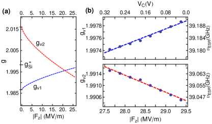
Figure 3: In (a) the valley $g$-factors are plotted depending on the electric field $F_{z}$, based on the model, Eqs. (63), (67), and (83), for each eigenvalley state: $|v_{1}\rangle$, $|v_{2}\rangle$. The $g$-factor offsets at zero field and the intercept at $F_{z}^{\rm int}\simeq 2.1\times 10^{7}\,{\rm V/m}$ are shown. In (b) the experimental electrical control over the valley $g$-factors is shown (dots, at a fixed magnetic field $B_{0}=1.4015\,{\rm T}$). The experimental points are fitted by the model, Eq. (83). Tuning both the confinement gate and the plunger gate at the QD Veldhorst et al. (2015b) provides control of the electric field $F_{z}$, and with that we can vary the qubit resonance frequency over several MHz. The experimentally observed opposite dependence of the valley $g$-factors on the electric field is attributed to the mixing of the original bulk degenerate spin-valley wave-functions at the $\rm Si/SiO_{2}$ interface, via the dominance of the inter-valley spin-flip contributions in the BC, Eqs. (6) and (11).

Finally, we would like to stress that the $g$-factor dependence of $F_{z}^{2/3}$ is for a high electric field (see Sec. III.2). Thus, we will model the low-field dependence in a simplistic way, by adding a (valley dependent) $g$-factor offset $\delta x_{v_{i}}$ (Fig. 3a):

$$g_{\rm v_{i}}=g_{\rm Si}^{*}+\delta x_{v_{i}}+A_{v_{i}}F_{z}^{2/3},$$ (83)

where $g_{\rm Si}^{*}\simeq 1.9983$ is the bulk value in Si for in-plane magnetic field Wilson and Feher (1960); Roth (1960); Liu (1962). By fitting Eq. (83) to the experimental data, Fig. 3b, one obtains the $g$-factor offsets $\delta x_{v_{1}}\simeq-0.012$, and $\delta x_{v_{2}}\simeq 0.018$ (with an error of $5\times 10^{-4}$), for this particular angle $\varphi=\pi/4$, when $B_{\|}$ is along the $[110]$-direction. We note, that the assumed $C_{\rm 2v}$-symmetry of the interface (quantum well) implies that the low-electric field Hamiltonian will be described by the same invariant Rashba and Dresselhaus structures, see Eq. (46). This would imply some $\sim\sin 2\varphi$ dependence of the offset values, reflecting the symmetry. A theory of the low-electric field effects in the $g$-factors, including offsets will be considered elsewhere.

While an interface with roughness (which is a realistic interface) will generally violate the “global” $C_{\rm 2v}$-symmetry, one might expect, for relatively small dots, a situation when the $C_{\rm 2v}$-symmetry is not violated within the quantum dot. This symmetry will dictate the form of the interface Hamiltonian, e.g in Eq. (46), and the $g$-factor angular dependence, derived in Eqs. (63) and (77). This physical intuition was recently confirmed experimentally, by observing the angular dependence in a Si-MOS DQD experiment Jock et al. (2018); Tanttu et al. (2018). Similar angular dependence was also revealed in a single QD with micromagnet, manipulated at a Si/Ge interface Ferdous et al. (2018a). We stress that any explicit violation of the $C_{\rm 2v}$-symmetry, (e.g., via explicit atomic step in the QD Ferdous et al. (2018b)) will not result in the angular dependence predicted here for the g-factor, Eq. (63); moreover, one would not be allowed to speak about Rashba and Dresselhaus contributions in the Hamiltonian. More experimental and theoretical work is needed to understand the role of atomic steps/roughness on the g-factor and other parameters.

IV.5.3 Spin-orbit coupled electric field noise

The $F_{z}$-dependence of the $g$-factor implies that a new dephasing mechanism is introduced via the fluctuations of the (gate) electric field, which was discussed in the context of 1e- and 3e- qubit using randomized benchmarking sequences to reveal it Magesan et al. (2012); Fogarty et al. (2015); Veldhorst et al. (2015b). For the single QD qubit of Ref. Veldhorst et al., 2015b this is the detuning noise $\delta\epsilon(t)$ of the Hamiltonian ${\cal H}_{Qb}=\frac{\epsilon}{2}\sigma_{z}+\frac{B_{1}^{\rm ac}}{2}\sigma_{x}$, where $\epsilon\propto\nu_{\rm ESR}-\nu_{v_{i}}$ is the detuning, and $B_{1}^{\rm ac}$ is the ac driving amplitude. Assuming a white noise, $\delta\epsilon(t)=\xi_{\epsilon}(t)$ with a (single-sided) noise spectral density $S_{\epsilon}$, (see, e.g. Ref. Korotkov, 2003), the dephasing rate $\gamma_{v_{i}}$ is derived at a chosen field $F_{z0}^{*}$ as

$$\gamma_{v_{i}}=\frac{S_{\epsilon}}{4\hbar^{2}}=\frac{(\mu_{B}B_{\parallel})^{2}}{4\hbar^{2}}\left|\frac{\partial[\delta g_{\parallel}^{v_{i}}(\varphi,F_{z0}^{*})]}{\partial F_{z}}\right|^{2}\,a^{2}\,S_{V},$$ (84)

where $S_{\epsilon}$ is linearly related to the gate voltage spectral density $S_{V}$, assuming linear dependence of field vs. voltage, $F_{z}\equiv a\,V$ (see, Fig. 3b and Ref. Yang et al., 2013). From Eq. (64) one obtains suppression for high fields, e.g., for a linear confinement: $\frac{\partial[\delta g_{\parallel}^{v_{i}}(\varphi,F_{z})]}{\partial F_{z}}=\frac{1}{F_{z}}\,\delta g_{\parallel}^{v_{i}}(\varphi,F_{z})$. Using Eq. (79), the dephasing rates for the 3e and 1e qubits (for $\varphi=\pi/4$) should be related as: $\gamma_{v_{2}}\simeq(2.24)^{2}\,\gamma_{v_{1}}$. On the other hand, using Hahn echo measurements one can cancel out the $1/f$ (drift) noise, and the measured $T_{2}$ reveals: $T_{2}^{3e}\approx 400\mu{s}$ and $T_{2}^{1e}\approx 1200\mu{s}$, i.e. a dephasing rate ratio of $3$ instead of $(2.24)^{2}$. This can be explained assuming another (valley-independent) dephasing $\gamma_{0}$ (it can be associated with some charge fluctuators or noise on the ac amplitude $B_{1}^{\rm ac}$). Thus, $\gamma_{3e}=\gamma_{v_{2}}+\gamma_{0}$, $\gamma_{1e}=\gamma_{v_{1}}+\gamma_{0}$, with $\gamma_{0}\simeq\gamma_{v_{1}}$, i.e. $\gamma_{0}$ is comparable to $\gamma_{v_{1}}$ in this experiment.

The quadratic dependence of the noise on the $g$-factor change: $S_{\epsilon}\propto[\delta g_{\parallel}^{v_{i}}(\varphi,F_{z})]^{2}$, Eqs. (64) and (84), implies that it can be zeroed at the “sweet spot angles” $\varphi_{v_{i}}$, defined in Eq. (65). At these angles (which may be different for the two eigenvalley subspaces, $v_{1},v_{2}$) either $\gamma_{1e}$ or $\gamma_{3e}$ will take the minimal value $\gamma_{0}$. Similar decrease of the noise can be achieved by rotating the field perpendicular to the interface, since the $g$-factor corrections are strongly suppressed, see Eqs. (75) and (76).

V Summary and Discussion

This paper presents a detailed theory to explain measurements of unexpected g-factor shifts in silicon quantum dots and to predict future experiments and impact to silicon-based quantum computing. We derived the effective spin-orbit interaction from appropriately formulated boundary conditions that take into account the symmetry of the silicon heterostructure interface and the hermiticity of the problem at hand. These effective spin-orbit interactions are used to derive the valley splitting at the interface, both its scaling with the applied electric field (perpendicular to the interface) and with the interface $z$-confinement for the conduction electrons. Then the 3D (and 2D) effective Rashba and Dresselhaus spin-orbit interactions are calculated, assuming a $C_{2v}$ interface symmetry. We argue that these new interface SOC contributions are much stronger than possible bulk contributions. Compared to previous phenomenological approaches Tahan et al. (2002); Friesen et al. (2007); Goswami et al. (2007); Shaji et al. (2008); Saraiva et al. (2009); Friesen and Coppersmith (2010); Culcer et al. (2010b, a); Rančić and Burkard (2016); Yang et al. (2013); Hao et al. (2014); Kawakami et al. (2014), the approach taken in this paper provides more rigorous ground for analyzing current and future experiments.

The effective spin-orbit interactions contain both diagonal (in the eigenvalley number) and off-diagonal contributions, which are to be used in the analysis of experiments that involve both eigenvalley states (e.g., in the so-called valley qubitsPrati (2011); Culcer et al. (2012)). Based on the above, we derived the electron $g$-factors for conduction 2DEG electrons (at a relatively weak lateral confinement) for an applied in-plane or perpendicular to the interface magnetic field. To leading order, we predicted the angular dependence of the $g$-factor with the in-plane angle, as well as with the azimuthal angle (for a magnetic field having a perpendicular component). For appropriate experiments with a single QD these predictions would allow us to extract the ratio of Rashba and Dresselhaus effective constants, from a measured $g$-factor angular dependence. In fact, any significant angular dependence will show that the Dresselhaus contribution dominates the Rashba one, thus supporting our statement that interface contributions are much stronger than that originating from the bulk.

The physical mechanism that causes shifts in the SOC parameters (and thus g-factor) as a function of electric field allows a new path for charge noise to affect the qubit. The predictions in this paper on the $g$-factor angular dependence are made for both lower and upper eigenvalley subspaces, which in general may have different spin-orbit (Rashba and Dresselhaus) contributions. We predict, based on the in-plane angular dependence, the so-called sweet spots in the direction of the magnetic field, when the $g$-factor correction, $\delta g$ is zero, and therefore there is no electric field scaling; consequently, the corresponding spin qubit would be insensitive (to first order) to the gate voltage (charge noise) of the applied electric field mediated by these new SOC contributions. As a trivial consequence, a QD qubit will be also insensitive to gate (charge) noise when the magnetic field is perpendicular to the interface, as in this case the $g$-factor variation is equally suppressed. To estimate this suppression, we have also calculated the second order corrections (in the perturbation theory) to the $g$-factor at any magnetic field direction, which also include the effects of the internal QD level structure, assuming strong confinement typical for the current experiments Veldhorst et al. (2014, 2015b); Hao et al. (2014); Jock et al. (2018); Tanttu et al. (2018). We have shown that these corrections are typically small $\sim 10^{-6}$ which supports the first order results discussed above. Eventually, an enhancement of these effects is possible near the so-called “relaxation hot spot” Yang et al. (2013), where the $g$-factor corrections may reach $\sim 10^{-4}-10^{-3}$, however such enhancement was not observed experimentally Veldhorst et al. (2014, 2015b). The absence of such enhancement may be explained (is consistent) with our theory, giving further constraints on the interface BC matrix parameters (both of their amplitudes and phases).

The ability to appreciably change the g-factor of an electron via applied voltages on top-gates offers a new and unplanned-for opportunity for control of silicon quantum dot qubits. For example, implementing a 2-qubit encoding Levy (2002) would allow for all-electrical control without the need for 3-quantum dots, magnetic field or nuclear gradients; this may be relevant for quantum computing not only in reducing the overhead in qubits but also in gate pulses as, for example, it has been recently showed that two-qubit encoded gates can be accomplished in far fewer gates than 2-DFS encodings Shim and Tahan (2016). Further, that one electron and three electron dots exhibit different behavior (while both still being good qubits), another opportunity exists for creative quantum dot gate protocols. On the other hand, g-factor tunability can create new mechanisms for decoherence, especially an increased sensitivity to charge noise. Our theory predicts a means to remove this channel by magic magnetic field angles (perpendicular for example). Finally, we note that the above theory should also apply to Si/Ge heterostructure quantum dots, with the caveat that the shift in g-factor will likely be smaller relative to the MOS-interface dots.

Note Added: Whilst we were preparing our manuscript Ruskov (2016); Tahan (2015) we became aware of a relevant experiment on a MOS double quantum dot system Jock et al. (2018) (and most recently see the experiment Tanttu et al. (2018)) at the similar conditions discussed in our paper, dealing with the lowest eigenvalley states in the DQD. Namely, their conditions are at an applied perpendicular to the interface electric field and at a magnetic field applied at various angles (both in-plane and perpendicular). The new experimental results of Ref. Jock et al., 2018 confirm to a large extent our predictions.

Particularly, (i) the very possibility to manipulate the Singlet-Triplet DQD qubit is via the difference in the electron $g$-factor in the two dots, which arises in the deep $(1,1)$ regime, where the electric field applied to each of the dots becomes essentially different (i.e., far from the symmetric/degeneracy point);
(ii) their observed angular dependence, $\sim\sin 2\varphi$ is compatible with our predictions for the lower eigenvalley subspace, see Eq. (63).
(iii) Since the difference of the Dresselhaus and Rashba effective spin orbit couplings, for the two dots, is linear with the dots’ electric field difference, the ratio of $\Delta\beta/\Delta\alpha\approx 8.3$ extracted in the DQD experiment Jock et al. (2018) is exactly the ratio of these couplings (that is independent of the electric field strength) $\beta_{D;v_{1}}/\alpha_{R;v_{1}}$, for the lower eigenvalley subspace, see Eqs. (47) and (48).
(iv) Finally, we mention that the predicted in our paper angular dependence of the dephasing, having a minimum dephasing rate at the “sweet spot angles”, Eq. (65), is yet to be measured in a future experiment.

Acknowledgments: A.S.D. acknowledges support from the Australian Research Council (CE11E0001017 and CE170100039) and the US Army Research Office (W911NF-13-1-0024 and W911NF-17-1-0198). The views and conclusions contained in this document are those of the authors and should not be interpreted as representing the official policies, either expressed or implied, of the Army Research Office or the U.S. Government. The U.S. Government is authorized to reproduce and distribute reprints for Government purposes notwithstanding any copyright notation herein.

Appendix A Derivation of the effective surface Hamiltonian from boundary conditions

In this appendix we derive Eq.(22). Starting with the boundary condition (6) one denotes it as ${\cal B}\Phi\mid_{z=z_{0}^{+}}=0$ with ${\cal B}\equiv{\cal B}_{1}+{\cal B}_{2}$, and ${\cal B}_{1}\equiv 1+iR\,k_{z}$, ${\cal B}_{2}\equiv-R\frac{2m_{l}}{\hbar^{2}}V_{\rm if}(\bm{k})$; $V_{\rm if}(\bm{k})$ being the interface spin-valley mixing matrix. Since $\langle k^{2}_{x,y}\rangle\ll\langle k^{2}_{z}\rangle$ (for a strong z-confinement) we will consider ${\cal B}_{2}$ as a perturbation. In what follows, we will approximately replace the boundary operator ${\cal B}$ by a unitary one up to higher order corrections:

$${\cal B}\simeq\Gamma_{BC},$$ (85)

with $\Gamma_{BC}\,\Gamma^{\dagger}_{BC}\simeq 1$.

Indeed, to zeroth order we have the BC ${\cal B}_{1}\Phi^{(0)}\mid_{z=z_{0}^{+}}=0$, see Eq.(32). Then it follows that

$${\cal B}_{2}\,{\cal B}_{1}\Phi^{(0)}\mid_{z=z_{0}^{+}}=0,$$ (86)

or

$${\cal B}_{2}\Phi^{(0)}\mid_{z=0^{+}}={\cal B}_{2}\,(1-{\cal B}_{1})\Phi^{(0)}\mid_{z=z_{0}^{+}}.$$ (87)

Now, to first order one have

$${\cal B}\Phi\mid_{z=z_{0}^{+}}=\Big{[}{\cal B}_{1}\,(\Phi^{(0)}+\Phi^{(1)})+{\cal B}_{2}\,\Phi^{(0)}\Big{]}\mid_{z=z_{0}^{+}}=0,$$ (88)

or

$$\Big{[}{\cal B}_{1}\,\Phi(z)+{\cal B}_{2}\,(1-{\cal B}_{1})\Phi(z)\Big{]}\mid_{z=z_{0}^{+}}=0,$$ (89)

where we have replaced $\Phi^{(0)}$ by $\Phi$ in the second term of Eq.(88) up to higher order corrections. The last BC, Eq.(89), can be rewritten in the form $\Gamma_{BC}\Phi(z)\mid_{z=z_{0}^{+}}=0$ where

$$\Gamma_{BC}={\cal B}_{1}+{\cal B}_{2}\,(1-{\cal B}_{1})=1+i\,\gamma_{BC}$$ (90)

$$\gamma_{BC}\equiv R\,k_{z}+R^{2}\frac{2m_{l}}{\hbar^{2}}V_{\rm if}(\bm{k})\,k_{z},$$ (91)

and $\Gamma_{BC}$ is an (approximate) unitary operator, $\Gamma_{BC}\,\Gamma^{\dagger}_{BC}=1+{\cal O}(\gamma_{BC}^{2})$, up to higher orders.

Performing now the unitary transform with $\Gamma_{BC}$ as in Eq.(21) the transformed BC is $\tilde{\Phi}\mid_{z=z_{0}^{+}}\equiv\Gamma_{\rm BC}\Phi\mid_{z=z_{0}^{+}}=0$ and the transformed Hamiltonian reads:

$$\tilde{{\cal H}}=\Gamma_{\rm BC}{\cal H}_{0}\Gamma^{\dagger}_{\rm BC}\simeq{\cal H}_{0}+\delta{\cal H}+{\cal O}(\gamma_{BC}^{2})$$

$$\delta{\cal H}=i\left[\gamma_{BC},{\cal H}_{0}\right]_{-}=R\partial_{z}U_{z}+R^{2}\frac{2m_{l}}{\hbar^{2}}V_{\rm if}(\bm{k})\partial_{z}U_{z}.$$ (92)

Appendix B QD level structure and its contribution to the $g$-factor

In order to emphasize the tunneling Hamiltonian representation implied by Eq. (5), we rewrite the expressions for the lowest eigenvalley states, Eq. (28), to the form

$$|\bar{v}_{i;\sigma}\rangle=\frac{1}{\sqrt{2}}\left[\begin{array}[]{c}C_{\sigma}\\ 0\end{array}\right]\,\phi^{+z}_{v_{i}}(\bm{r})+\left(\frac{\mp e^{-i\phi_{V}}}{\sqrt{2}}\right)\left[\begin{array}[]{c}0\\ C_{\sigma}\end{array}\right]\,\phi^{-z}_{v_{i}}(\bm{r})\quad\ \$$ (97)

$$i=1,2\,;\ \ \sigma=\uparrow,\downarrow,$$

where the corresponding valley populations are $\alpha_{+z}^{v_{1}}=\frac{1}{\sqrt{2}}$, $\alpha_{-z}^{v_{1}}=-e^{-i\phi_{V}}\frac{1}{\sqrt{2}}$, $\alpha_{+z}^{v_{2}}=\frac{1}{\sqrt{2}}$, $\alpha_{-z}^{v_{2}}=+e^{-i\phi_{V}}\frac{1}{\sqrt{2}}$. Time reversal maintains the relations: $|\alpha_{+z}^{v_{j}}|=|\alpha_{-z}^{v_{j}}|$ and $\phi_{v_{j}}^{+z}\bm{r})=\phi_{v_{j}}^{-z}\bm{r})$. For the lowest energy envelopes $\phi^{+z}_{v_{i}}(\bm{r})=\phi^{v_{i}}_{0}(x,y)\,\varphi_{0}(z)$ the dependence on the eigenvalley index $v_{i}$ is due to interface roughness (atomic steps within the dot), and makes $\phi^{v_{i}}_{0}(x,y)$ to acquire a $p$-like contributionYang et al. (2013); Gamble et al. (2013). The corresponding four lowest states $|v_{i}\rangle\otimes|0_{x},0_{y},0_{z}\rangle\otimes|\sigma\rangle\equiv|\bar{v}_{i},\sigma\rangle$, are enumerated as: $|1\rangle\equiv|\bar{v}_{1},\downarrow\rangle$, $|2\rangle\equiv|\bar{v}_{1},\uparrow\rangle$, $|3\rangle\equiv|\bar{v}_{2},\downarrow\rangle$, $|4\rangle\equiv|\bar{v}_{2},\uparrow\rangle$, see Sec. IV.2.2. The higher orbital states, Fig. 1d, $|v_{i}\rangle\otimes|1_{x},0_{y},0_{z}\rangle\otimes|\sigma\rangle$, $|v_{i}\rangle\otimes|0_{x},1_{y},0_{z}\rangle\otimes|\sigma\rangle$, are enumerated using the notations $|m_{1}\rangle\equiv|v_{1}\rangle\otimes|1_{x},0_{y},0_{z}\rangle$, $|m_{2}\rangle\equiv|v_{1}\rangle\otimes|0_{x},1_{y},0_{z}\rangle$, and $|\tilde{m}_{1}\rangle$, $|\tilde{m}_{2}\rangle$ for $v_{1}\to v_{2}$, namely: $|5\rangle\equiv|m_{1},\downarrow\rangle$, $|6\rangle\equiv|m_{1},\uparrow\rangle$, $|7\rangle\equiv|m_{2},\downarrow\rangle$, $|8\rangle\equiv|m_{2},\uparrow\rangle$, $|9\rangle\equiv|\tilde{m}_{1},\downarrow\rangle$, $|10\rangle\equiv|\tilde{m}_{1},\uparrow\rangle$, $|11\rangle\equiv|\tilde{m}_{2},\downarrow\rangle$, $|12\rangle\equiv|\tilde{m}_{2},\uparrow\rangle$, see Sec. IV.2.2. The roughness effects for these states are neglected. Also, higher orbital states are not considered assuming a close-to-parabolic lateral confinement.

We consider the valley diagonal SOC Hamiltonian Eq. (54) in a 3D form [since the 2D SOC Hamiltonians are generally inconsistent with the extension of derivatives]. By suitably rotating the axes for an in-plane magnetic field, $\bm{B}_{\parallel}=(B_{x},B_{y},0)$ one obtains

$${\cal H}_{v_{i}}=\left[\alpha_{R;v_{i}}\,\left\{\left(s\tilde{\sigma}_{x}+c\tilde{\sigma}_{z}\right)P_{y}+\left(c\tilde{\sigma}_{x}-s\tilde{\sigma}_{z}\right)P_{x}\right\}\right.$$

$$\left.{}+\beta_{D;v_{i}}\,\left\{\left(s\tilde{\sigma}_{x}+c\tilde{\sigma}_{z}\right)P_{y}+\left(c\tilde{\sigma}_{x}-s\tilde{\sigma}_{z}\right)P_{x}\right\}\right]\,\frac{\partial_{z}U_{z}}{\hbar\langle\partial_{z}U_{z}\rangle},$$ (98)

where $s\equiv\sin\varphi$, $c\equiv\cos\varphi$, $\bm{P}=\hbar\bm{k}+|e|\bm{A}$ are the extended derivatives, $B_{x}=B\cos\varphi$, $B_{y}=B\sin\varphi$, and the Pauli matrices along the new axes are

$$\tilde{\sigma}_{z}=\frac{\sigma_{x}B_{x}+\sigma_{y}B_{y}}{B},\ \ \tilde{\sigma}_{x}=\frac{\sigma_{x}B_{y}-\sigma_{y}B_{x}}{B}$$ (99)

with $\tilde{\sigma}_{z}|\uparrow,\downarrow\rangle=\pm|\uparrow,\downarrow\rangle$, $\tilde{\sigma}_{x}|\uparrow,\downarrow\rangle=|\downarrow,\uparrow\rangle$.

Taking the matrix elements $V_{kk}=\langle k|{\cal H}_{v_{1}}|k\rangle,\,k=1,2$ one obtains for the first order correction to the g-factor ($U_{z}=|e|F_{z}z$ for simplicity):

$$\delta^{(1)}g^{v_{1}}_{\|}=\frac{V_{22}-V_{11}}{\mu_{B}B}=-\frac{|e|}{\hbar\mu_{B}}\langle z\rangle\left(\alpha_{R;v_{1}}-\beta_{D;v_{1}}\,\sin 2\varphi\right).$$ (100)

It is straightforward to see that for a 3-electron QD, one can write the wave function as a Slater determinant (mean field approximation is implicit Culcer et al. (2010a); Bakker et al. (2015)), where two of the electrons are occupying the lowest orbital $|\bar{v}_{1}\rangle$, and the “valence” electron occupies the upper (split by $E_{\rm VS}$) orbital, $|\bar{v}_{2}\rangle$, Fig. 1c. Then, the matrix element over the 3e wave function is reduced to a single-particle matrix element of the form: $V_{kk}=\langle k|{\cal H}_{v_{2}}|k\rangle,\,k=3,4$, which leads to the expression for $\delta^{(1)}g^{v_{2}}_{\|}$ analogous to Eq. (100), with the replacement $v_{1}\to v_{2}$.

B.1 Second order corrections: case of $\bm{B}_{\parallel}$

For the second order corrections it is convenient to introduce compact notations for the SOC constants, Eqs. (47)-(50): $a_{ii}\equiv\alpha_{R;v_{i}}$, $b_{ii}\equiv\beta_{D;v_{i}},\ i=1,2$, and $a_{21}\equiv\alpha_{R;21}$, $b_{21}\equiv\beta_{D;21}$. The second order corrections include transitions to higher states with different valley content; so, both diagonal and non-diagonal in valley SOC Hamiltonians, Eq.(46), contribute:

$${\cal H}_{\rm s-v}^{ij}=\frac{a_{ij}}{\hbar}\,\left(\sigma_{x}P_{y}-\sigma_{y}P_{x}\right)+\frac{b_{ij}}{\hbar}\,\left(\sigma_{x}P_{x}-\sigma_{y}P_{y}\right).$$ (101)

Rotating the axes as above, one obtains for the first few matrix elements

$$V_{12}=\langle\bar{v}_{1},\downarrow|{\cal H}_{\rm s-v}|\bar{v}_{1},\uparrow\rangle$$

$${}=\hbar^{-1}\langle\phi^{v_{1}}(\bm{x})|a_{11}\left(cP_{x}+sP_{y}\right)+b_{11}\left(sP_{x}+cP_{y}\right)|\phi^{v_{1}}(\bm{x})\rangle\quad$$ (102)

$$V_{13}=\langle\bar{v}_{1},\downarrow|{\cal H}_{\rm s-v}|\bar{v}_{2},\downarrow\rangle$$

$${}=\hbar^{-1}\langle\phi^{v_{1}}(\bm{x})|a_{12}\left(sP_{x}-cP_{y}\right)-b_{12}\left(cP_{x}-sP_{y}\right)|\phi^{v_{2}}(\bm{x})\rangle\quad$$ (103)

$$V_{14}=\langle\bar{v}_{1},\downarrow|{\cal H}_{\rm s-v}|\bar{v}_{2},\uparrow\rangle$$

$${}=\hbar^{-1}\langle\phi^{v_{1}}(\bm{x})|a_{12}\left(cP_{x}+sP_{y}\right)+b_{12}\left(sP_{x}+cP_{y}\right)|\phi^{v_{2}}(\bm{x})\rangle\quad$$ (104)

$$V_{15}=\langle\bar{v}_{1},\downarrow|{\cal H}_{\rm s-v}|m_{1},\downarrow\rangle$$

$${}=\hbar^{-1}\langle\phi^{v_{1}}(\bm{x})|a_{11}\left(sP_{x}-cP_{y}\right)-b_{11}\left(cP_{x}-sP_{y}\right)|\phi^{m_{1}}(\bm{x})\rangle\qquad$$ (105)

$$V_{16}=\langle\bar{v}_{1},\downarrow|{\cal H}_{\rm s-v}|m_{1},\uparrow\rangle$$

$${}=\hbar^{-1}\langle\phi^{v_{1}}(\bm{x})|a_{11}\left(cP_{x}+sP_{y}\right)+b_{11}\left(sP_{x}+cP_{y}\right)|\phi^{m_{1}}(\bm{x})\rangle\!,\ \ \qquad$$ (106)

etc. The matrix elements $V_{ab},\ a=1,2,\,b=1,\ldots,12$, are routinely calculated, using the relation between momentum and position matrix elements via the equation of motion. For example,

$$\langle\phi^{v_{1}}(\bm{x})|p_{x}|\phi^{m}(\bm{x})\rangle=\frac{im_{t}}{\hbar}\langle\phi^{v_{1}}(\bm{x})|\left[{\cal H}_{\rm tot},x\right]_{-}|\phi^{m}(\bm{x})\rangle$$

$$\qquad{}=\frac{im_{t}}{\hbar}\left(E_{1}-E_{m}\right)\,\langle\phi^{v_{1}}(\bm{x})|\,x\,|\phi^{m}(\bm{x})\rangle,$$ (107)

and similarly for $\langle p_{y}\rangle$.

Using these relations and the gauge $\bm{A}_{\|}(\bm{r})=(B_{y}z,-B_{x}z,0)$, we calculate the matrix elements

$$V_{12}=-\frac{|e|}{\hbar}\beta_{D;v_{1}}\,\cos 2\varphi\,\langle z\rangle\quad\ \$$ (108)

$$V_{13}=\left\{\frac{a_{12}}{\hbar}\left[\frac{im_{t}}{\hbar}E_{\rm VS}\left(cy_{12}-sx_{12}\right)-B\,\langle z\rangle\right]\right.$$

$$\qquad\left.{}+\frac{b_{12}}{\hbar}\left[\frac{im_{t}}{\hbar}E_{\rm VS}\left(cx_{12}-sy_{12}\right)-B\sin 2\varphi\,\langle z\rangle\right]\right\}\quad\ \$$ (109)

$$V_{14}=\left\{-\frac{a_{12}}{\hbar}\left[\frac{im_{t}}{\hbar}E_{\rm VS}\left(cx_{12}+sy_{12}\right)\right]\right.$$

$$\qquad\left.{}-\frac{b_{12}}{\hbar}\left[\frac{im_{t}}{\hbar}E_{\rm VS}\left(cy_{12}+sx_{12}\right)+|e|B\cos 2\varphi\,\langle z\rangle\right]\right\}\quad\quad$$ (110)

$$V_{15}=\left\{\frac{\alpha_{R;v_{1}}}{\hbar}\left[\frac{im_{t}}{\hbar}\Delta_{\rm orb}\left(cy_{1,m_{1}}-sx_{1,m_{1}}\right)\right]\right.$$

$$\qquad\left.{}+\frac{\beta_{D;v_{1}}}{\hbar}\left[\frac{im_{t}}{\hbar}\Delta_{\rm orb}\left(cx_{1,m_{1}}-sy_{1,m_{1}}\right)\right]\right\}\quad\ \$$ (111)

$$V_{16}=\left\{-\frac{\alpha_{R;v_{1}}}{\hbar}\left[\frac{im_{t}}{\hbar}\Delta_{\rm orb}\left(cx_{1,m_{1}}+sy_{1,m_{1}}\right)\right]\right.$$

$$\qquad\left.{}-\frac{\beta_{D;v_{1}}}{\hbar}\left[\frac{im_{t}}{\hbar}\Delta_{\rm orb}\left(cy_{1,m_{1}}+sx_{1,m_{1}}\right)\right]\right\}\quad\ \$$ (112)

The remaining matrix elements, $V_{17},\ldots,V_{1,12}$ can be obtained from $V_{15}$, $V_{16}$ by suitable replacements of the envelopes: $V_{17}=V_{15}(m_{1}\to m_{2})$, $V_{18}=V_{16}(m_{1}\to m_{2})$, $V_{19}=V_{15}(m_{1}\to\tilde{m}_{1},\Delta_{\rm orb}\to\Delta_{\rm orb}+E_{\rm VS})$, $V_{1,10}=V_{16}(m_{1}\to\tilde{m}_{1},\Delta_{\rm orb}\to\Delta_{\rm orb}+E_{\rm VS})$, $V_{1,11}=V_{19}(m_{1}\to\tilde{m}_{2})$, $V_{1,12}=V_{1,10}(m_{1}\to\tilde{m}_{2})$. For the second series of matrix elements, they are related to the above one (for in-plane magnetic field, $\bm{B}_{\|}$). Thus, $V_{23}=V_{14}$, $V_{24}=-V_{13}$, $V_{25}=V_{16}$, $V_{26}=-V_{15}$, etc. $\ldots\,,V_{2,12}=-V_{1,11}$.

Using standard 2nd-order perturbation theory for the energy difference $[\delta E_{2}^{(2)}-\delta E_{1}^{(2)}]$ and the above relations one gets:

$$\delta E_{2}^{(2)}-\delta E_{1}^{(2)}=\frac{2|V_{12}|^{2}}{E_{Z}}+|V_{14}|^{2}\left(\frac{1}{E_{Z}-E_{\rm VS}}+\frac{1}{E_{Z}+E_{\rm VS}}\right)$$

$$\quad\quad{}+2|V_{16}|^{2}\left(\frac{1}{E_{Z}-\Delta_{\rm orb}}+\frac{1}{E_{Z}+\Delta_{\rm orb}}\right)$$

$$\ \ {}+2|V_{1,10}|^{2}\left(\frac{1}{E_{Z}-\Delta_{\rm orb}-E_{\rm VS}}+\frac{1}{E_{Z}+\Delta_{\rm orb}+E_{\rm VS}}\right),$$ (113)

and for the g-factor one obtains, by grouping the terms:

$$\delta E_{2}^{(2)}-\delta E_{1}^{(2)}=\delta^{(2)}\!g_{\|}^{v_{1}}\,\,\mu_{B}B$$

$$\delta^{(2)}\!g_{\|}^{v_{1}}\equiv\delta g^{12}_{\|}+\delta g^{14}_{\|}+\delta g^{16}_{\|}+\delta g^{1,10}_{\|}.\quad\ \ \$$ (114)

The relevant contributions read:

$$\delta g^{12}_{\|}=\frac{|e|^{2}}{\hbar^{2}\mu_{B}^{2}}\frac{2}{g^{*}}\beta^{2}_{D;v_{1}}\,\cos^{2}2\varphi\,\langle z\rangle^{2}$$ (115)

$$\delta g^{14}_{\|}=-\frac{|e|^{2}}{\hbar^{2}\mu_{B}^{2}}\frac{1}{E_{\rm VS}^{2}-E_{Z}^{2}}\left\{\frac{2}{g^{*}}\,E_{Z}^{2}\,b_{12}^{2}\,\cos^{2}2\varphi\,\langle z\rangle^{2}+\frac{g^{*}}{2}E_{\rm VS}^{2}\right.$$

$$\left.{}\qquad\times\frac{m_{t}^{2}}{m_{0}^{2}}\left[a_{12}\left(cx_{12}+sy_{12}\right)+b_{12}\left(cy_{12}+sx_{12}\right)\right]^{2}\right\}$$ (116)

$$\delta g^{16}_{\|}+\delta g^{18}_{\|}=-\frac{|e|^{2}}{\hbar^{2}\mu_{B}^{2}}\frac{g^{*}}{2}\frac{m_{t}^{2}}{m_{0}^{2}}\frac{\Delta^{2}_{\rm orb}}{\Delta^{2}_{\rm orb}-E_{Z}^{2}}$$

$$\times\left\{y_{1,m_{1}}^{2}\left[s\,\alpha_{R;v_{1}}+c\,\beta_{D;v_{1}}\right]^{2}+x_{1,m_{2}}^{2}\left[c\,\alpha_{R;v_{1}}+s\,\beta_{D;v_{1}}\right]^{2}\right\}\quad\$$ (117)

$$\delta g^{1,10}_{\|}+\delta g^{1,12}_{\|}=-\frac{|e|^{2}}{\hbar^{2}\mu_{B}^{2}}\frac{g^{*}}{2}\frac{m_{t}^{2}}{m_{0}^{2}}\frac{\left(\Delta_{\rm orb}+E_{\rm VS}\right)^{2}}{\left(\Delta_{\rm orb}+E_{\rm VS}\right)^{2}-E_{Z}^{2}}$$

$$\quad\times\left\{y_{1,\tilde{m}_{1}}^{2}\left[s\,a_{12}+c\,b_{12}\right]^{2}+x_{1,\tilde{m}_{2}}^{2}\left[c\,a_{12}+s\,b_{12}\right]^{2}\right\}.$$ (118)

In the above, we have used (for a circular dot with parabolic confinement) that: $x_{1,m_{1}}=y_{1,m_{2}}=x_{1,\tilde{m}_{1}}=y_{1,\tilde{m}_{2}}=0$. The standard non-zero dipole matrix elements to orbital states, $y_{1,m_{1}}=x_{1,m_{2}}=y_{1,\tilde{m}_{1}}=x_{1,\tilde{m}_{2}}=\sqrt{\frac{\hbar^{2}}{2m_{t}\Delta_{\rm orb}}}$ will be used for further evaluation of Eqs. (117) and (118).

B.2 Second order corrections: case of $\bm{B}_{\perp}$

For the second order corrections in perpendicular magnetic field $\bm{B}_{\perp}$ we use the SOC Hamiltonians Eq. (101) and include transitions to higher states as was done above. One obtains for the first few matrix elements

$$V_{12}=\langle\bar{v}_{1},\downarrow|{\cal H}_{\rm s-v}|\bar{v}_{1},\uparrow\rangle$$

$${}=\hbar^{-1}\langle\phi^{v_{1}}(\bm{x})|a_{11}\left(P_{y}-iP_{x}\right)+b_{11}\left(P_{x}-iP_{y}\right)|\phi^{v_{1}}(\bm{x})\rangle\qquad$$ (119)

$$V_{13}=0$$ (120)

$$V_{14}=\langle\bar{v}_{1},\downarrow|{\cal H}_{\rm s-v}|\bar{v}_{2},\uparrow\rangle$$

$${}=\hbar^{-1}\langle\phi^{v_{1}}(\bm{x})|a_{12}\left(P_{y}-iP_{x}\right)+b_{12}\left(P_{x}-iP_{y}\right)|\phi^{v_{2}}(\bm{x})\rangle\qquad$$ (121)

$$V_{15}=0$$ (122)

$$V_{16}=\langle\bar{v}_{1},\downarrow|{\cal H}_{\rm s-v}|m_{1},\uparrow\rangle$$

$${}=\hbar^{-1}\langle\phi^{v_{1}}(\bm{x})|a_{11}\left(P_{y}-iP_{x}\right)+b_{11}\left(P_{x}-iP_{y}\right)|\phi^{m_{1}}(\bm{x})\rangle,\qquad$$ (123)

etc. The structure of the higher matrix elements is similar, e.g., $V_{17}=V_{19}=V_{1,11}=0$, $V_{18}=V_{16}(m_{1}\to m_{2})$, $V_{1,10}=V_{16}(m_{1}\to\tilde{m}_{1})$, $V_{1,12}=V_{16}(m_{1}\to\tilde{m}_{2})$. For the second series of matrix elements, they are related to the above one (for perpendicular magnetic field, $\bm{B}_{\perp}$) Thus, $V_{23}=V_{14}(i\to-i)$, $V_{25}=V_{16}(i\to-i)$, $V_{27}=V_{18}(i\to-i)$, $V_{29}=V_{1,10}(i\to-i)$, $V_{2,11}=V_{1,12}(i\to-i)$. For the squared matrix elements, these replacements correspond to the formal sign change of $E_{Z}=g^{*}\mu_{B}B$ (see below).

Using standard 2nd-order perturbation theory for the energy difference $[\delta E_{2}^{(2)}-\delta E_{1}^{(2)}]$ and the above relations one gets:

$$\delta E_{2}^{(2)}-\delta E_{1}^{(2)}=\frac{2|V_{12}|^{2}}{E_{Z}}+\left(\frac{|V_{23}|^{2}}{E_{Z}-E_{\rm VS}}+\frac{|V_{14}|^{2}}{E_{Z}+E_{\rm VS}}\right)$$

$${}+\left(\frac{|V_{25}|^{2}}{E_{Z}-\Delta_{\rm orb}}+\frac{|V_{16}|^{2}}{E_{Z}+\Delta_{\rm orb}}\right)+(m_{1}\to m_{2})$$

$${}+\left(\frac{|V_{29}|^{2}}{E_{Z}-\Delta_{\rm orb}-E_{\rm VS}}+\frac{|V_{1,10}|^{2}}{E_{Z}+\Delta_{\rm orb}+E_{\rm VS}}\right)$$

$${}+(\tilde{m}_{1}\to\tilde{m}_{2}).$$ (124)

The matrix elements $V_{ab},\ a=1,2,\,b=1,\ldots,12$, are calculated similar to the previous case, using the equation of motion, Eq. (107).

Having at hand these matrix elements, we use the 2nd-order correction to the energy difference, Eq. (124), and group the terms accordingly:

$$\delta E_{2}^{(2)}-\delta E_{1}^{(2)}=\delta^{(2)}\!g_{\perp}^{v_{1}}\,\,\mu_{B}B$$

$$\delta^{(2)}\!g_{\perp}^{v_{1}}\equiv\delta g^{12}_{\perp}+\delta g^{14}_{\perp}+\delta g^{16}_{\perp}+\delta g^{18}_{\perp}+\delta g^{1,10}_{\perp}+\delta g^{1,12}_{\perp}.\quad\ \ \$$ (125)

The relevant contributions to $\delta^{(2)}\!g_{\perp}$ read:

$$\delta g^{12}_{\perp}=\frac{|e|^{2}}{\hbar^{2}\mu_{B}^{2}}\frac{1}{2g^{*}}\left\{\left(x_{11}\alpha_{R;v_{1}}-y_{11}\beta_{D;v_{1}}\right)^{2}\right.$$

$$\qquad\qquad\qquad\quad\quad\left.{}+\left(x_{11}\beta_{D;v_{1}}-y_{11}\alpha_{R;v_{1}}\right)^{2}\right\}\qquad\quad$$ (126)

which coincides with Eq. (75), as expected. Also,

$$\delta g^{14}_{\perp}=\frac{g^{*}}{E_{Z}}\left[\frac{|V_{14}|^{2}}{E_{Z}+E_{\rm VS}}+\frac{|V_{23}|^{2}}{E_{Z}-E_{\rm VS}}\right]=\frac{|e|^{2}}{4\hbar^{2}\mu_{B}^{2}}\frac{1}{h_{z}\left(\frac{m_{0}}{m_{t}}+2h_{z}\right)}$$

$$\qquad\times\left\{\left[x_{12}\,a_{12}(1-h_{z})+y_{12}\,b_{12}(1+h_{z})\right]^{2}\right.$$

$$\qquad\qquad\ \left.{}+\left[x_{12}\,b_{12}(1+h_{z})+y_{12}\,a_{12}(1-h_{z})\right]^{2}\right\}$$

$$\qquad{}+(h_{z}\to-h_{z})$$ (127)

with $h_{z}\equiv\frac{m_{0}}{m_{t}}\frac{E_{Z}}{2E_{VS}}$.

$$\delta g^{16}_{\perp}+\delta g^{18}_{\perp}=\frac{g^{*}}{E_{Z}}\left[\frac{|V_{16}|^{2}}{E_{Z}+\Delta_{\rm orb}}+\frac{|V_{25}|^{2}}{E_{Z}-\Delta_{\rm orb}}\right]+(m_{1}\to m_{2})\qquad$$

$$\qquad\qquad\ \ \ {}=\frac{|e|^{2}}{4\hbar^{2}\mu_{B}^{2}}\frac{1}{\tilde{h}_{z}\left(\frac{m_{0}}{m_{t}}+2\tilde{h}_{z}\right)}\left\{\left(y_{1,m_{1}}^{2}+x_{1,m_{2}}^{2}\right)\right.$$

$$\qquad\qquad\qquad\left.\times\left(\alpha_{R;v_{1}}^{2}(1-\tilde{h}_{z})^{2}+\beta_{D;v_{1}}^{2}(1+\tilde{h}_{z})^{2}\right)\right\}$$

$$\qquad\qquad\quad{}+(\tilde{h}_{z}\to-\tilde{h}_{z})$$ (128)

with $\tilde{h}_{z}\equiv\frac{m_{0}}{m_{t}}\frac{E_{Z}}{2\Delta_{\rm orb}}$.

$$\delta g^{1,10}_{\perp}+\delta g^{1,12}_{\perp}=\frac{g^{*}}{E_{Z}}\left[\frac{|V_{1,10}|^{2}}{E_{Z}+\Delta_{\rm orb}+E_{\rm VS}}+\frac{|V_{29}|^{2}}{E_{Z}-\Delta_{\rm orb}-E_{\rm VS}}\right]$$

$$\ {}+(\tilde{m}_{1}\to\tilde{m}_{2})=\frac{|e|^{2}}{4\hbar^{2}\mu_{B}^{2}}\frac{1}{\bar{h}_{z}\left(\frac{m_{0}}{m_{t}}+2\bar{h}_{z}\right)}\left\{\left(y_{1,\tilde{m}_{1}}^{2}+x_{1,\tilde{m}_{2}}^{2}\right)\right.$$

$$\qquad\qquad\qquad\quad\left.\times\left(a_{12}^{2}(1-\bar{h}_{z})^{2}+b_{12}^{2}(1+\bar{h}_{z})^{2}\right)\right\}$$

$$\qquad\qquad\qquad{}+(\bar{h}_{z}\to-\bar{h}_{z})$$ (129)

with $\bar{h}_{z}\equiv\frac{m_{0}}{m_{t}}\frac{E_{Z}}{2\left(\Delta_{\rm orb}+E_{\rm VS}\right)}$. In the above, we have used the relations for the dipole matrix elements to orbital states, see text after Eqs. (117) and (118).

As mentioned above, for an interface with roughness the lowest energy envelopes, $\phi^{v_{i}}(x,y)$ (quasi s-like) acquire a p-like contribution, depending on the eigenvalley index $v_{i}$. Thus, the dipole matrix elements $\bm{r}_{ij}\equiv\langle v_{i}|\bm{r}|v_{j}\rangle$ $i,j=1,2$ are generally non-zero Yang et al. (2013); Gamble et al. (2013), getting size of few nm for this type of QDsYang et al. (2013).

B.3 $\delta g$ at the spin-valley anticrossing point

At the anticrossing (at the so-called “relaxation hot spot”)Yang et al. (2013), when $E_{Z}\approx E_{\rm VS}$, the contribution $\delta g^{14}_{\|}$ acquires a first order correction (by solving the standard secular equation). The exact qubit energy difference is $\frac{1}{2}\left[E_{\rm VS}+E_{Z}-\sqrt{\left(E_{\rm VS}-E_{Z}\right)^{2}+\Delta_{a}^{2}}\right]$, where

$$\Delta_{a}=2|V_{23}|=2|V_{14}|$$ (130)

is the splitting at anticrossing of the relevant valley statesYang et al. (2013); Hao et al. (2014) $|2\rangle$ and $|3\rangle$, see Eqs. (110), (121), and Fig. 1d. Close to anticrossing, when $\delta\equiv E_{\rm VS}-E_{Z}\lesssim\Delta_{a}$,

$$\delta g_{\rm hot-spot}=-\frac{\Delta_{a}}{E_{Z}}+\frac{\delta}{E_{Z}}-\frac{\delta^{2}}{2\Delta_{a}E_{Z}}.$$ (131)

Thus $\delta g_{\rm hot-spot}$ may be of the order of $10^{-3}$ or less since the splitting was evaluated Yang et al. (2013); Hao et al. (2014) as $\Delta_{a}=(10^{-3}-10^{-4})\,E_{\rm VS}$. This is at least $~{}10$ times smaller than the observed experimental $g$-factor correction Veldhorst et al. (2014, 2015b), as presented on Fig. 3. Also, there is no any observed deviation from the linear dependence with $F_{z}$ near the anticrossing point which restricts the size of $\Delta_{a}$.

B.4 The integral relation, Eq. (30), for a $z$-confinement potential $U(z)$ with an infinite boundary

One starts with the one-dimensional eigenvalue problem

$$-\frac{\hbar^{2}}{2m}\varphi^{\prime\prime}(z)+U(z)\varphi(z)-E\varphi(z)=0$$ (132)

with $\varphi(0)=0$. By multiplying Eq. (132) by ${\varphi^{*}}^{\prime}(z)$ and integrating by parts the first and last term:

$$\int_{0}^{\infty}dz{\varphi^{*}}^{{}^{\prime}}(z)\varphi^{\prime\prime}(z)=-{\varphi^{*}}^{\prime}(0)\varphi^{\prime}(0)-\int_{0}^{\infty}dz{\varphi^{*}}^{\prime\prime}(z)\varphi^{\prime}(z)\qquad\ \$$ (133)

$$-E\,\int_{0}^{\infty}dz{\varphi^{*}}^{\prime}(z)\varphi(z)=E\,\int_{0}^{\infty}dz\varphi^{*}(z)\varphi^{\prime}(z),$$ (134)

then one adds the conjugate 1D-equation, multiplied by $\varphi^{\prime}(z)$. As a result, $-\int_{0}^{\infty}dz\frac{2m}{\hbar^{2}}U(z)\frac{d}{dz}|\varphi(z)|^{2}=|\varphi^{\prime}(0)|^{2}$ or

$$\frac{2m}{\hbar^{2}}\,\int_{0}^{\infty}dz\varphi^{*}(z)\partial_{z}U(z)\varphi(z)=|\varphi^{\prime}(0)|^{2}.$$ (135)

Appendix C Interface boundary condition from hermiticity of the Hamiltonian

C.1 Volkov-Pinsker boundary condition

For completeness, we first re-derive the Volkov-Pinsker BC Volkov and Pinsker (1979), starting from single-band approximation Hamiltonian, in the presence of external field, $\bm{A}(\bm{r})$:

$${\cal H}=\frac{(\bm{p}+|e|\bm{A})^{2}}{2m}+U(\bm{r}).$$ (136)

Considering two arbitrary solutions, $\phi_{1}$, $\phi_{2}$ of the Schrödinger equation, one states the hermiticity condition at the half-space, $z>z_{0}$ Volkov and Pinsker (1979):

$$\int_{z>z_{0}}dz\,\phi_{1}^{\dagger}\left({\cal H}\phi_{2}\right)=\int_{z>z_{0}}dz\,\phi_{2}\left({\cal H}\phi_{1}\right)^{*}.$$ (137)

Substituting ${\cal H}$ in Eq. (137,) and integrating by parts one gets the relation (put $\hbar=e=1$):

$$\phi_{2}(z_{0})\frac{d\phi_{1}^{*}}{dz}-\phi_{1}^{*}(z_{0})\frac{d\phi_{2}}{dz}+2i\phi_{1}^{*}(z_{0})A_{z}(z_{0})\phi_{2}(z_{0})=0,$$ (138)

where separation of variables is assumed for the potential, Eq.(18). Eq. (138) can be satisfied if

$$\frac{1}{\phi_{1}}\frac{d\phi_{1}(z_{0})}{dz}=\frac{1}{\phi_{2}}\frac{d\phi_{2}(z_{0})}{dz}={\it const.}+iA_{z}(z_{0}).$$ (139)

By choosing ${\it const.}\equiv-\frac{1}{R}$ one can recast Eq. (139) to the BC:

$$\left\{1+i\frac{R}{\hbar}\left(p_{z}+|e|A_{z}\right)\right\}\,\phi(z)\mid_{z_{0}^{+}}=0,$$ (140)

with $p_{z}\equiv-i\hbar\partial_{z}$. For $A_{z}=0$ one recovers Eq.(8). As follows from Eq. (140), the gauge invariance of the Schrodinger equation plus boundary conditions implies in general “extension of derivatives” both in the Hamiltonian and in the boundary conditions. In case of the spin-valley BCs considered in the main text, Eqs. (6), (19), and (55), one should extent both the $\partial_{z}$-derivative as well as the $\partial_{x,y}$-derivatives.

Notice also that the bulk velocity operator is $v_{z}\equiv\frac{\partial{\cal H}}{\partial p_{z}}=\frac{1}{m}\left(p_{z}+|e|A_{z}\right)$. The hermiticity condition, Eq. (138) then can be rewritten as

$$\phi_{1}^{*}\left(v_{z}\phi_{2}\right)+\left(v_{z}\phi_{1}\right)^{*}\phi_{2}\,\mid_{z_{0}^{+}}=0.$$ (141)

This implies continuity of the envelope flux density, despite of the discontinuity of the wave function at its derivative at the interface.

C.2 BC and gauge-invariance

Concerning the gauge invariance, we have already mentioned in Sec. IV.1 that the problem (Hamiltonian plus boundary conditions) is written in a gauge invariant form, via the extension of the derivatives. Therefore, in the actual calculations, one is using the most convenient gauge as is, e.g., with the results for the $g$-factor renormalization, Eqs. (57)-(67). One may ask the question how the gauge invariance is preserved during the derivation, e.g., of Eq. (67)? One mention that any gauge change leads to a multiplication of the wave function with a phase factor, which cancels in the quantum average $\langle z\rangle$ in Eq. (67) [considering a boundary at $z_{0}=0$]. By using the gauge $\bm{A}_{\|}(\bm{r})=(z,-z,0)B/\sqrt{2}$, for each of the two spin components, there is a modification of the $z$-confinement potential of Eq. (18) by a linear $z$-term. This leads to a modification of the eigenvalues of the original problem, Eq. (14), which ends up with the result Eq. (67) as a first order correction. Since we are considering a homogeneous magnetic field, the vector potential is a linear function of the coordinates, including also an arbitrary constant vector. E.g., for the gauge $\bm{A}^{\prime}=\bm{A}_{\|}(\bm{r})+(c,-c,0)$ one naively would expect a shift in the $z$-coordinate. This gauge transformation, however, corresponds to adding a constant to the Hamiltonian Eq. (14), which does not change the eigenvalues. Thus, the gauge invariance is preserved in this case.

One may consider the gauge $\bm{A}^{\prime\prime}=(0,0,y-x)B/\sqrt{2}$, which is more involved. Indeed, in this case there is no explicit $z$, and one is puzzling how one can obtain the $\langle z\rangle$ in the final result. One starts with the BC, Eq. (6) in the form

$$\left\{1+iR(k_{z}+\frac{|e|}{\hbar}A_{z})-R\,\frac{2m_{l}}{\hbar^{2}}\,V_{\rm if}(\bm{k})\right\}\Phi(\bm{r})\mid_{z=0^{+}}$$

$$\qquad\qquad\qquad\qquad\qquad\equiv{\cal B}(A_{z})\Phi(\bm{r})\mid_{z=0^{+}}=0,$$ (142)

and following the derivations of Eqs. (21) and (22), one obtains the effective unitary transform (see Appendix A)

$$\Gamma_{BC}(A_{z})=1+i\left[R(k_{z}+\frac{|e|}{\hbar}A_{z})+R^{2}\frac{2m_{l}}{\hbar^{2}}V_{\rm if}(\bm{k})(k_{z}+\frac{|e|}{\hbar}A_{z})\right]$$ (143)

such that $\Gamma_{BC}(A_{z})\Phi(\bm{r})\mid_{z=0^{+}}\simeq 0$. After some elaborate calculation, using the above described procedure, one can obtain a term in the effective Hamiltonian perturbation, $\Delta H$, which is $~{}k_{z}^{2}$. Thus, since $\langle k_{z}^{2}\rangle={\it const.}\langle z\rangle$ for the triangular potential in Eq. (14), and $\langle z\rangle$ is recovered.

C.3 Estimation of the R parameter

One can illustrate how an effective length parameter $R$ appears in a single-band BC like Eq. (140) from a two-band modelVolkov and Pinsker (1979), with 2-component envelope, $\phi^{T}=[\phi_{c}(\bm{r}),\phi_{v}(\bm{r})]$, including conduction and valence bands. Neglecting ${\cal O}(p_{z}^{2})$ effects, the $\bm{k}\cdot\bm{p}$-Hamiltonian is

$${\cal H}^{\rm 2band}=\left(\begin{array}[]{cc}E_{c}&\frac{p_{\rm cv}}{m_{0}}\,p_{z}\\ \frac{p^{*}_{\rm cv}}{m_{0}}\,p_{z}&E_{v}\end{array}\right),$$ (144)

where $p_{\rm cv}$ is the interband momentum matrix element. The BC, Eq. (141), is recasted to $(-\phi_{1v}^{*}\,\phi_{2c}+\phi_{1c}^{*}\,\phi_{2v})\mid_{z_{0}^{+}}=0$, for any two functions, $\phi_{1}$, $\phi_{2}$. On the other hand, a stationary solution of the Schrödinger equation with ${\cal H}^{\rm 2band}$ gives a relation: $\phi_{c}=-\frac{p_{\rm cv}p_{z}}{(E_{c}-E)m_{0}}\phi_{v}$ (and analogous one, with $c\to v$), allowing to exclude the other band. (It is worth to stress here, that such relations make it impossible to have simultaneously $\phi_{c}(z_{0})=0$ and $\phi_{v}(z_{0})=0$, as required by the standard BC with infinite boundary). Compatibility of the two-band BC with the single-band BC, Eq. (140), leads to the relationVolkov and Pinsker (1979): $R_{c}\simeq R_{v}=\frac{1}{2}\,\sqrt{\frac{2\hbar^{2}}{m_{c}^{*}E_{\rm gap}}}$, where $E_{\rm gap}=E_{c}-E_{v}\approx 4\,{\rm eV}$ is the band gap in Si at the band minima, $m_{c}^{*}$ is the effective mass, and we have used the approximate relation Yu and Cardona (2010): $\frac{m_{0}}{m_{c}^{*}}\approx\frac{2p_{\rm cv}^{2}}{m_{0}E_{\rm gap}}$. Thus, as a rough estimation (i.e., not taking into account valleys) one gets $R=R_{c}^{\rm Si}\approx 0.1-0.2\,{\rm nm}$ for $m_{t}<m_{c}^{*}<m_{l}$.

References

- Rashba and Sheka (1991) E. I. Rashba and V. I. Sheka, Electric-Dipole Spin Resonances In: Landau Level Spectroscopy, Edited by G. Landwehr and E. I. Rashba (Elsevier Science Publishers B.V., Amsterdam, 1991).
- Datta and Das (1990) S. Datta and B. Das, Appl. Phys. Lett. 56, 665 (1990).
- Hasan and Kane (2010) M. Hasan and C. Kane, Rev. Mod. Phys. 82, 3045 (2010).
- Jansen (2012) R. Jansen, Nature Materials 11, 400 (2012).
- Zwanenburg et al. (2013) F. Zwanenburg, A. S. Dzurak, A. Morello, M. Y. Simmons, L. C. L. Hollenberg, G. Klimeck, S. Rogge, S. N. Coppersmith, and M. A. Eriksson, Rev. Mod. Phys. 85, 961 (2013).
- Maune et al. (2012) B. M. Maune, M. G. Borselli, B. Huang, T. D. Ladd, P. W. Deelman, K. S. Holabird, A. A. Kiselev, I. Alvarado-Rodriguez, R. S. Ross, A. E. Schmitz, M. Sokolich, C. A. Watson, M. F. Gyure, and A. T. Hunter, Nature 481, 344 (2012).
- Yang et al. (2013) C. H. Yang, A. Rossi, R. Ruskov, N. S. Lai, F. A. Mohiyaddin, S. Lee, C. Tahan, G. Klimeck, A. Morello, and A. S. Dzurak, Nat. Commun. 4, 2069 (2013).
- Hao et al. (2014) X. Hao, R. Ruskov, M. Xiao, C. Tahan, and H. Jiang, Nat. Commun. 5, 3860 (2014).
- Kim et al. (2014) D. Kim, Z. Shi, C. B. Simmons, D. R. Ward, J. R. Prance, T. S. Koh, J. K. Gamble, D. E. Savage, M. G. Lagally, M. Friesen, S. N. Coppersmith, and M. A. Eriksson, Nature 511, 70 (2014).
- Kawakami et al. (2014) E. E. Kawakami, P. Scarlino, D. R. Ward, F. R. Braakman, D. E. Savage, M. G. Lagally, M. Friesen, S. N. Coppersmith, M. A. Eriksson, and L. M. K. Vandersypen, Nature Nanotechnology 9, 666 (2014).
- Veldhorst et al. (2014) M. Veldhorst, J. C. C. Hwang, C. H. Yang, A. W. Leenstra, B. de Ronde, J. P. Dehollain, J. T. Muhonen, F. E. Hudson, K. M. Itoh, A. Morello, and A. S. Dzurak, Nature Nanotechnology 9, 981 (2014).
- Veldhorst et al. (2015a) M. Veldhorst, C. H. Yang, J. C. C. Hwang, W. Huang, J. Dehollain, J. Muhonen, S. Simmons, A. Laucht, F. Hudson, K. Itoh, A. Morello, and A. Dzurak, Nature 526, 410 (2015a).
- Veldhorst et al. (2015b) M. Veldhorst, R. Ruskov, C. H. Yang, J. C. C. Hwang, F. E. Hudson, M. E. Flatté, C. Tahan, K. M. Itoh, A. Morello, and A. S. Dzurak, Phys. Rev. B 92, 201401(R) (2015b).
- Ferdous et al. (2018a) R. Ferdous, E. Kawakami, P. Scarlino, M. P. Nowak, D. R. Ward, D. E. Savage, M. G. Lagally, S. N. Coppersmith, M. Friesen, M. A. Eriksson, L. M. K. Vandersypen, and R. Rahman, NPJ Quantum Information 4, 26 (2018a).
- Ferdous et al. (2018b) R. Ferdous, K. W. Chan, M. Veldhorst, J. C. C. Hwang, C. H. Yang, H. Sahasrabudhe, G. Klimeck, A. Morello, A. S. Dzurak, and R. Rahman, Phys. Rev. B 97, 241401(R) (2018b).
- Jock et al. (2018) R. M. Jock, N. T. Jacobson, P. Harvey-Collard, A. M. Mounce, V. Srinivasa, D. R. Ward, J. Anderson, R. Manginell, J. R. Wendt, M. Rudolph, T. Pluym, J. K. Gamble, A. D. Baczewski, W. M. Witzel, and M. S. Carroll, Nature Communications 9, 1768 (2018).
- Corna et al. (2018) A. Corna, L. Bourdet, R. Maurand, A. Crippa, D. Kotekar-Patil, H. Bohuslavskyi, R. Lavieville, L. Hutin, S. Barraud, X. Jehl, M. Vinet, S. De Franceschi, Y.-M. Niquet, and M. Sanquer, NPJ Quantum Information 4, 6 (2018).
- Tanttu et al. (2018) T. Tanttu, B. Hensen, K. W. Chan, H. Yang, W. Huang, M. A. Fogarty, F. E. Hudson, K. M. Itoh, D. Culcer, A. Laucht, A. Morello, and A. S. Dzurak, “Controlling spin-orbit interactions in silicon quantum dots using magnetic field direction,” (2018), arXiv:1807.10415v3 [cond-mat] .
- Itoh and Watanabe (2014) K. M. Itoh and H. Watanabe, MRS Communications 4, 143 (2014).
- Roth (1960) L. M. Roth, Phys. Rev. 118, 1534 (1960).
- Liu (1962) L. Liu, Phys. Rev. 126, 1317 (1962).
- Ohkawa and Uemura (1977a) F. J. Ohkawa and Y. Uemura, Journal of the Physical Society of Japan 43, 907 (1977a).
- Sham and Nakayama (1979) L. J. Sham and M. Nakayama, Phys. Rev. B 20, 734 (1979).
- Friesen et al. (2007) M. Friesen, S. Chutia, C. Tahan, and S. N. Coppersmith, Phys. Rev. B 75, 115318 (2007).
- Nestoklon et al. (2008) M. O. Nestoklon, E. L. Ivchenko, J. -M. Jancu, and P. Voisin, Phys. Rev. B 77, 155328 (2008).
- Saraiva et al. (2009) A. L. Saraiva, M. J. Calderón, X. Hu, S. Das Sarma, and B. Koiller, Phys. Rev. B 80, 081305(R) (2009).
- Ivchenko and Kiselev (1992) E. L. Ivchenko and A. A. Kiselev, Sov. Phys. Semiconductors-USSR 26, 827 (1992).
- Kiselev et al. (1998) A. A. Kiselev, E. L. Ivchenko, and U. Rössler, Phys. Rev. B 58, 16353 (1998).
- Vasko and Prima (1981) F. T. Vasko and N. A. Prima, Fiz. Tverdogo Tela 23, 2042 (1981).
- Rodina et al. (2003) A. V. Rodina, A. L. Efros, and A. Y. Alekseev, Phys. Rev. B 67, 155312 (2003).
- Rodina and Alekseev (2006) A. V. Rodina and A. Y. Alekseev, Phys. Rev. B 73, 115312 (2006).
- Kiselev et al. (1997) A. A. Kiselev, E. L. Ivchenko, and M. Willander, Solid State Commun. 102, 375 (1997).
- Jancu et al. (2005) J. -M. Jancu, R. Scholz, E. A. de Andrada e Silva, and G. C. La Rocca, Phys. Rev. B 72, 193201 (2005).
- Volkov and Pinsker (1979) V. A. Volkov and T. N. Pinsker, Surface Science 81, 181 (1979).
- Vasko and Kuznetsov (1998) F. T. Vasko and A. V. Kuznetsov, Electronic States and Optical Transitions in Semiconductor Heterostructures (Springer, New York, 1998).
- Ando and Mori (1982) T. Ando and S. Mori, Surface Science 113, 124 (1982).
- Tokatly et al. (2002) I. V. Tokatly, A. G. Tsibizov, and A. A. Gorbatsevich, Phys. Rev. B 65, 165328 (2002).
- Braginsky (1999) L. S. Braginsky, Phys. Rev. B 60, R13970 (1999).
- Devizorova and Volkov (2014) Z. A. Devizorova and V. A. Volkov, JETP Letters 100, 102 (2014).
- Gamble et al. (2013) J. K. Gamble, M. A. Eriksson, S. N. Coppersmith, and M. Friesen, Phys. Rev. B 88, 035310 (2013).
- Ohkawa and Uemura (1977b) F. J. Ohkawa and Y. Uemura, Journal of the Physical Society of Japan 43, 917 (1977b).
- Ohkawa (1978) F. J. Ohkawa, Solid State Commun. 26, 69 (1978).
- Boykin et al. (2004) T. B. Boykin, G. Klimeck, M. Friesen, S. N. Coppersmith, P. von Allmen, F. Oyafuso, and S. Lee, Phys. Rev. B 70, 165325 (2004).
- Nestoklon et al. (2006) M. O. Nestoklon, L. E. Golub, and E. L. Ivchenko, Phys. Rev. B 73, 235334 (2006).
- Golub and Ivchenko (2004) L. E. Golub and E. L. Ivchenko, Phys. Rev. B 69, 115333 (2004).
- Kohn and Luttinger (1955) W. Kohn and J. M. Luttinger, Phys. Rev. 98, 915 (1955).
- Vasko (1979) F. T. Vasko, JETP Letters 30, 541 (1979).
- Braginsky (1998) L. S. Braginsky, Phys. Rev. B 57, R6870 (1998).
- Tamm (1932) I. E. Tamm, Phys. Z. Sowjetunion 1, 733 (1932).
- Note (1) For ideal quantum well interfaces the relevant interface symmetry ( or ) admits only the invariant structure corresponding to a Dresselhaus contribution Golub and Ivchenko (2004), while with an applied perpendicular electric field the reduced symmetry admits also the Rashba structure.
- Culcer et al. (2010a) D. Culcer, X. Hu, and S. Das Sarma, Phys. Rev. B 82, 205315 (2010a).
- Friesen and Coppersmith (2010) M. Friesen and S. N. Coppersmith, Phys. Rev. B 81, 115324 (2010).
- Note (2) Interference effects similar to that in Refs. Nestoklon et al. (2006, 2008) will be considered elsewhere.
- (54) For a interface, with a valley splittingYang et al. (2013) , and estimated SOC couplings, Eqs. (81) and (82), one gets , with .
- (55) Using the tight-binding resultFriesen et al. (2007) for the valley splitting parameter: , one gets at for a interface .
- (56) For arbitrary interface position , the -dependence cancels in the phase differences, , , as required by translational invariace .
- (57) These BCs, Eq. (55), are similar to that derived for single-valley heterostructures with an abrupt interface Rodina and Alekseev (2006); Devizorova and Volkov (2014) .
- Wilson and Feher (1960) D. Wilson and G. Feher, Bull. Am. Phys. Soc. 5, 60 (1960).
- Ruskov (2016) R. Ruskov, “Invited talk at the Silicon quantum electronics conference, Delft, The Netherlands, June 13-14,” (2016).
- Tahan (2015) C. Tahan, “Talk at the Quantum Computing Program Review, San Diego, CA, Aug 10-12,” (2015).
- Note (3) R. Ferdous, R. Rahman, private communication.
- Magesan et al. (2012) E. Magesan, J. M. Gambetta, B. R. Johnson, C. A. Ryan, J. M. Chow, S. T. Merkel, M. P. da Silva, G. A. Keefe, M. B. Rothwell, T. A. Ohki, M. B. Ketchen, and M. Steffen, Phys. Rev. Lett. 109, 080505 (2012).
- Fogarty et al. (2015) M. A. Fogarty, M. Veldhorst, R. Harper, C. H. Yang, S. D. Bartlett, S. T. Flammia, and A. S. Dzurak, Phys. Rev. A 92, 022326 (2015).
- Korotkov (2003) A. N. Korotkov, Phys. Rev. B 67, 235408 (2003).
- Tahan et al. (2002) C. Tahan, M. Friesen, and R. Joynt, Phys. Rev. B 66, 035314 (2002).
- Goswami et al. (2007) S. Goswami, K. A. Slinker, M. Friesen, L. M. McGuire, J. L. Truitt, C. Tahan, L. J. Klein, J. O. Chu, P. M. Mooney, D. W. van Derweide, R. Joynt, S. N. Coppersmith, and M. A. Eriksson, Nat. Phys. 3, 41 (2007).
- Shaji et al. (2008) N. Shaji, C. B. Simmons, M. Thalakulam, L. J. Klein, H. Qin, H. Luo, D. E. Savage, M. G. Lagally, A. J. Rimberg, R. Joynt, M. Friesen, R. H. Blick, S. N. Coppersmith, and M. A. Eriksson, Nat Phys 4, 540 (2008).
- Culcer et al. (2010b) D. Culcer, L. Cywiński, Q. Li, X. Hu, and S. Das Sarma, Phys. Rev. B 82, 155312 (2010b).
- Rančić and Burkard (2016) M. J. Rančić and G. Burkard, Phys. Rev. B 93, 205433 (2016).
- Prati (2011) E. Prati, Journal of Nanoscience and nanotechnology 11, 8522 (2011).
- Culcer et al. (2012) D. Culcer, A. L. Saraiva, B. Koiller, X. Hu, and S. Das Sarma, Phys. Rev. Lett. 108, 126804 (2012).
- Levy (2002) J. Levy, Phys. Rev. Lett. 89, 147902 (2002).
- Shim and Tahan (2016) Y.-P. Shim and C. Tahan, Phys. Rev. B 93, 121410(R) (2016).
- Bakker et al. (2015) M. A. Bakker, S. Mehl, T. Hiltunen, A. Harju, and D. P. DiVincenzo, Phys. Rev. B 91, 155425 (2015).
- Yu and Cardona (2010) P. Yu and M. Cardona, Fundamentals of Semiconductors (Springer, Berlin, 2010).