Butterfly Velocities for Holographic Theories of General Spacetimes

Yasunori Nomura^a,b,c and Nico Salzetta^a,b

^a Berkeley Center for Theoretical Physics, Department of Physics,
University of California, Berkeley, CA 94720, USA

^b Theoretical Physics Group, Lawrence Berkeley National Laboratory, CA 94720, USA

^c Kavli Institute for the Physics and Mathematics of the Universe (WPI), University of Tokyo, Kashiwa, Chiba 277-8583, Japan

1 Introduction

The quantum theory of gravity is expected to be formulated in a non-gravitational spacetime whose dimension is less than that of the bulk gravitational spacetime [1, 2, 3]. The holographic theories for general spacetimes are not explicitly known, but we expect that they are strongly coupled based on the known holographic correspondence between conformal field theories (CFT) and quantum gravity in asymptotically anti-de Sitter (AdS) spacetimes [4]. If cosmological spacetimes do indeed admit holographic descriptions, it is critical to find the appropriate dual theories in order to understand the quantum nature of gravity in our universe. In an effort to find such theories, we take a bottom-up approach and calculate quantities that can help identify them.

A particular quantity that characterizes a strongly coupled system is the butterfly velocity [5, 6, 7], which can be viewed as the effective speed of the spread of information relevant for an ensemble of states. Recently, Qi and Yang [8] generalized the concept to general subspaces of a Hilbert space, including a code subspace of a holographic theory [9, 10]. They then discussed its relationship to the causal structure of an emergent bulk theory.

In this paper, we investigate butterfly velocities in holographic theories of general spacetimes, described in Refs. [11, 12]. In particular, we calculate butterfly velocities for bulk local operators in the holographic theory of cosmological flat Friedmann-Robertson-Walker (FRW) spacetimes and analyze their properties. We find that they admit a certain universal scaling, independent of the fluid component and the dimension of the bulk spacetime. This emerges in the limit that the boundary region representing a bulk operator becomes small, where we expect that the butterfly velocity reflects properties of the underlying theory.

We also provide an extension of the prescription of Ref. [8] for computing the butterfly velocity to include more general operators in the bulk. This generalization allows us to calculate the butterfly velocities of bulk local operators in some entanglement shadow regions.

Together with the monotonicity property of the change of the volume of the holographic space [13, 14, 15] and the behavior of the entanglement entropies of subregions of a holographic space [11, 16], our results provide important data for finding explicit holographic theories of general spacetimes. In particular, our results seem to indicate a certain relation between spatial and temporal scaling in the holographic theory of flat FRW spacetimes.

The organization of the paper is as follows. In Section 2, we define the butterfly velocity in holographic theories and discuss (extended) prescriptions of calculating it using the bulk effective theory. In Section 3, we compute butterfly velocities in the holographic theory of flat FRW universes and analyze their properties. In Section 4, we discuss possible implications of our results.

Throughout the paper, we take units where the bulk Planck length is unity. We assume that the bulk spacetime satisfies the null and causal energy conditions. These impose the conditions $\rho\geq-p$ and $|\rho|\geq|p|$, respectively, on the energy density $\rho$ and pressure $p$ of an ideal fluid component, so that the equation of state parameter, $w=p/\rho$, satisfies $|w|\leq 1$.

2 Definition of the Butterfly Velocity in Holographic Theories of General Spacetimes

We are interested in the spread of information in holographic theories of general spacetimes. The butterfly velocity is a quantity that characterizes the spread of correlations of operators acting within a certain subspace of a Hilbert space. In particular, we can restrict our attention to a code subspace of states in which observables correspond to operators acting within the bulk effective theory.

We work within the framework described in Ref. [11]. The theory is defined on the holographic spacetime, which for a fixed semiclassical bulk spacetime corresponds to a holographic screen [17], a special codimension-1 surface in the bulk. The holographic screen is uniquely foliated by surfaces called leaves; this corresponds to a fixed time slicing of the holographic theory. We study how the support of an operator dual to a bulk local operator spreads in time. In Section 2.1, we follow Ref. [8] and define the butterfly velocity in this context. We then describe how to calculate it using the bulk effective theory. We also discuss conceptual issues associated with this procedure. In Section 2.2, we extend the definition to include bulk operators in entanglement shadows.

2.1 Butterfly velocities on holographic screens

We are interested in how the support of a holographic representation of a bulk local operator, ${\cal O}$, changes in time in the holographic theory.

This analysis is complicated by the fact that each bulk local operator can be represented in multiple ways in the holographic space (which we may loosely refer to as the boundary, borrowing from AdS/CFT language) [18, 19, 20]. For example, suppose the operator is represented over the whole boundary, as in the global representation in AdS/CFT. There is then no concept of the operator spreading in time. Following Ref. [8], we avoid this issue by representing a bulk operator at a point $p$ such that $p$ is on the Hubeny-Rangamani-Takayanagi (HRT) surface [21] of a subregion of the boundary. Specifically, we consider a subregion $A$ on a leaf $\sigma_{0}$ (not of an arbitrary spatial section of the holographic screen) and represent a bulk local operator ${\cal O}$ located on the HRT surface, $\gamma_{A}$, of $A$. Based on intuition arising from analyzing tensor network models [10, 22], we expect that such a representation is unique. We denote the operator in the boundary theory represented in this way on $A$ as ${\cal O}_{A}$.

We want to know the spatial region $B$ on the leaf $\sigma_{\varDelta t}$, which is in the future of $\sigma_{0}$ by time $\varDelta t$, such that every operator ${\cal B}$ supported on $B$ satisfies

$$\langle\Psi_{i}|[{\cal O}_{A},{\cal B}]|\Psi_{j}\rangle=0.$$ (1)

Here, $|\Psi_{i}\rangle$ and $|\Psi_{j}\rangle$ are arbitrary states in the code subspace. Recall that there is a natural way of relating regions on different leaves of a holographic screen [15]. The spatial coordinates on $\sigma_{\varDelta t}$ can be defined from those on $\sigma_{0}$ by following the integral curves of a vector field orthogonal to every leaf on the holographic screen. We can then define the region $A^{\prime}$ on $\sigma_{\varDelta t}$ corresponding to $A$ on $\sigma_{0}$ by following such curves. This allows us to define the distance, $\varDelta d$, of the operator spread for each point $q$ on the boundary, $\partial A^{\prime}$, of $A^{\prime}$ as the distance from $q$ to the region $B$ in the direction orthogonal to $\partial A^{\prime}$.

For an arbitrary operator in $A$, there is no reason that the distance $\varDelta d$ is independent of the location on $\partial A^{\prime}$. The butterfly velocity can then be defined using the largest of $\varDelta d$ along $\partial A^{\prime}$ [8]:

$$v_{B}\equiv\underset{\theta_{i}}{\rm max}\frac{\varDelta d}{\varDelta t},$$ (2)

where $\{\theta_{i}\}$ are the coordinates of $q$ on $\partial A^{\prime}$.

We now discuss how to calculate $v_{B}$ using the bulk effective theory. For this, we must understand how time evolved operators in the bulk are represented in the boundary theory. More specifically, given a particular representation, ${\cal O}_{A}$, of ${\cal O}$ in the holographic Hilbert space, what representation of the time evolved bulk operator (within the light cone of $p$) does the time evolution of ${\cal O}_{A}$ corresponds to? Without an explicit boundary theory it is not possible to answer this question, but we can still make some headway using intuition. First, we may expect that the region $B$ on $\sigma_{\varDelta t}$ (defined above) fully excludes $A^{\prime}$. This is the statement that the support of the operator does not shrink in any direction. Second, we want the “minimal necessary extension” of the leaf subregion $A$. For instance, it seems unphysical that a bulk operator represented on subregion $A$ should immediately time evolve into the full boundary representation of the future bulk operator. We thus seek the correspondingly “maximal” region $B$ whose entanglement wedge does not contain the interior of light cone of $p$. Excluding the light cone ensures that no information can be sent in the bulk which would compromise the commutativity between ${\cal O}_{A}$ and ${\cal B}$ within the code subspace.

From these considerations, we come up with two possible procedures for calculating the butterfly velocity of a bulk operator at a point $p$:

1. Maximize the volume of subregion $B^{\prime}$ subject to the constraint that $A^{\prime}\cap B^{\prime}=\emptyset$ and that the entanglement wedge of $B^{\prime}$ does not contain the interior of the light cone of $p$. The resulting subregion then gives $B$.

2. Find the subregion $B$ with the distance from $\partial B$ to $\partial A^{\prime}$ being both minimal and independent of the location on $\partial B$, again subject to the constraint that the entanglement wedge of $B$ does not contain the light cone of $p$.

One can certainly consider other possibilities as well, but these are the two most intuitively obvious candidates. However, we find that the first possibility leads to discontinuous behavior of $B$ as $p$ moves across the tip of the HRT surface of a spherical cap region. We therefore focus on the second possibility, which aligns with Ref. [8].

Essentially, this possibility postulates that the support of the operator ${\cal O}_{A}$ spreads uniformly:

$$\frac{\partial\varDelta d}{\partial\theta_{i}}=0.$$ (3)

We assume that this is indeed the case. The prescription of calculating the butterfly velocity can then be given explicitly as follows. We first consider a region $B^{\prime}(\varDelta\lambda)$ on $\sigma_{\varDelta t}$ which is (i) $\varDelta\lambda$ away from $A^{\prime}$, i.e. the distance from any point on $\partial A^{\prime}$ to $B^{\prime}(\varDelta\lambda)$ is $\varDelta\lambda$ in the direction orthogonal to $\partial A^{\prime}$ and (ii) the entanglement wedge of $B^{\prime}(\varDelta\lambda)$ does not contain the interior of the light cone of $p$. The butterfly velocity of ${\cal O}_{A}$ is then obtained by finding $B^{\prime}(\varDelta\lambda)$ with the smallest $\varDelta\lambda$

$$v_{B}=\underset{\varDelta\lambda}{\rm min}\frac{\varDelta\lambda}{\varDelta t}.$$ (4)

Note that the resulting $v_{B}$ depends on how the bulk operator ${\cal O}$ is represented initially, i.e. $A$ and the location of ${\cal O}$ on $\gamma_{A}$.

If the assumption of Eq. (3) is not valid in general, then our results for the “off-center” operators, $f\neq 0$, in Section 3 (as well as any related results in Ref. [8]) would have to be reinterpreted as representing something other than $v_{B}$ defined in Eq. (2). However, our results for the operators at the tip of the HRT surface, $f=0$, are still correct in this case, since Eq. (3) is guaranteed by the symmetry of the setup.

2.2 Bulk operators in entanglement shadows

In the prescription given in the previous subsection, the bulk operator ${\cal O}$ was on the HRT surface of a subregion $A$ on a leaf. Motivated by the idea that a bulk local operator can be represented in the holographic theory not only at an intersection of HRT surfaces but also at an intersection of the edge of the entanglement wedges (associated with subregions of leaves) [12, 25], we expect that we can similarly calculate the butterfly velocity for an operator ${\cal O}_{A}$ corresponding to a bulk operator at a point $p$ on the boundary of the entanglement wedge of $A$, ${\rm EW}(A)$.

There is no obstacle in using either of the prescriptions detailed in the previous subsection, except now we take $p$ to be on the edge of the entanglement wedge. In this case, we must be careful to exclude the entire light cone of $p$ when finding $B$. We find that the behavior of $v_{B}$ is qualitatively different depending on whether $p$ is on the future or past boundary of ${\rm EW}(A)$.

Suppose $p$ is on the past boundary of ${\rm EW}(A)$. In this case, ${\rm EW}(B)$ is not limited by excluding the part of $p$’s light cone infinitesimally close to $p$ (as is the case when $p$ is on $\gamma_{A}$), but by the part of the light cone that is just to the future of $\gamma_{A}$. Aside from this, there is no other new aspect compared with the case in which $p$ is on $\gamma_{A}$. In particular, $A^{\prime}$ is forced to spread relative to $A$ in both prescriptions.

There is, however, a subtlety when $p$ is on the future boundary of ${\rm EW}(A)$. This arises because ${\rm EW}(\bar{A^{\prime}})$ automatically excludes the light cone of points located on the future boundary of ${\rm EW}(A)$. Here, $\bar{A^{\prime}}$ is the complement of $A^{\prime}$ on $\sigma_{\varDelta t}$. A direct application of the first prescription from the previous subsection would then result in a butterfly velocity of $0$ for bulk operators at all points on the future boundary of ${\rm EW}(A)$. This is due to the constraint that $A^{\prime}\cap B=\emptyset$, forcing $v_{B}\geq 0$. This constant $v_{B}=0$ behavior may encourage us to abandon the constraint, but doing so leads to severely discontinuous behavior of $B$. Namely, the resulting region $B$ on $\sigma_{\varDelta t}$ is independent of the original region $A$ on $\sigma_{0}$, because $B$ will always find the same global maximum.

The second prescription has more interesting behavior so long as we allow for the distance from $\partial B$ to $\partial A^{\prime}$ to be negative. Doing so, we see that $B$ is now constrained by excluding the past light cone of $p$, and for the resulting $B$, $A^{\prime}\cap B\neq\emptyset$, so that $v_{B}\leq 0$. This is interesting because as we move forward in the boundary time, we are actually tracking the past time evolution of a bulk local operator. The shrinking support of ${\cal O}_{A}$ could indicate that this is a finely tuned boundary operator.

This generalization to the boundary of entanglement wedges allows us to calculate the butterfly velocity of operator ${\cal O}_{A}$ representing a bulk local operator in an entanglement shadow, i.e. a spacetime region in which HRT surfaces do not probe.

3 Butterfly Velocities for the Holographic Theory of FRW Universes

In this section, we compute butterfly velocities for the holographic theory of $(3+1)$-dimensional flat Friedmann-Robertson-Walker (FRW) universes:

$$ds^{2}=a^{2}(\eta)\bigl{[}-d\eta^{2}+dr^{2}+r^{2}(d\psi^{2}+\sin^{2}\!\psi\,d\phi^{2})\bigr{]},$$ (5)

where $a(\eta)$ is the scale factor with $\eta$ being the conformal time. We mainly focus on the case in which a universe is dominated by a single ideal fluid component with the equation of state parameter $w=p/\rho$ with $|w|\leq 1$.

In Section 3.1, we derive an analytic expression for the butterfly velocity of a bulk local operator near the holographic screen. In Section 3.2, we numerically calculate the butterfly velocity for a bulk operator located at the tip of an HRT surface with an arbitrary depth. In Section 3.3, we extend the result of Section 3.1 to arbitrary spacetime dimensions.

3.1 Local operators near the holographic screen

Consider a spherical cap region

$$\Gamma:0\leq\psi\leq\gamma,$$ (6)

on the leaf at a time $\eta_{*}$, which is located at

$$r=\frac{a(\eta)}{\dot{a}(\eta)}\biggr{|}_{\eta=\eta_{*}}\equiv r_{*}.$$ (7)

Following Ref. [11], we go to cylindrical coordinates:

$$\xi=r\sin\psi,\qquad z=r\cos\psi-r_{*}\cos\gamma,$$ (8)

in which the boundary of $\Gamma$, $\partial\Gamma$, is located at

$$\xi=r_{*}\sin\gamma\equiv\xi_{*},\qquad z=0.$$ (9)

In the case that $\gamma\ll 1$, i.e. $\xi_{*}\ll r_{*}$, the HRT surface anchored to $\partial\Gamma$ can be expressed in a power series form. Denoting the surface by $\eta$ and $z$ as functions of $\xi$, we find

$$\eta(\xi)= \eta_{*}+\eta^{(2)}(\xi)+\eta^{(4)}(\xi)+\cdots,$$ (10)

$$z(\xi)= 0,$$ (11)

where

$$\eta^{(2)}(\xi)= \frac{\dot{a}}{2a}(\xi_{*}^{2}-\xi^{2}),$$ (12)

$$\eta^{(4)}(\xi)= -\frac{\dot{a}}{16a^{3}}(\xi_{*}^{2}-\xi^{2})\bigl{\{}4\dot{a}^{2}\xi_{*}^{2}-a\ddot{a}(3\xi_{*}^{2}-\xi^{2})\bigr{\}},$$ (13)

with

$$a\equiv a(\eta_{*}),\qquad\dot{a}\equiv\frac{da(\eta)}{d\eta}\biggr{|}_{\eta=\eta_{*}},\qquad\ddot{a}\equiv\frac{d^{2}a(\eta)}{d\eta^{2}}\biggr{|}_{\eta=\eta_{*}}.$$ (14)

We consider a bulk local operator on this surface.

We parameterize the location, $p$, of the operator by a single number $f$ ($0\leq f<1$) representing how much fractionally the operator is “off the center,” i.e. the operator is located on the surface

$$\psi=f\gamma,$$ (15)

with $\eta$ and $r$ determined by the condition that it is also on the HRT surface of Eq. (10); see Fig. 1.

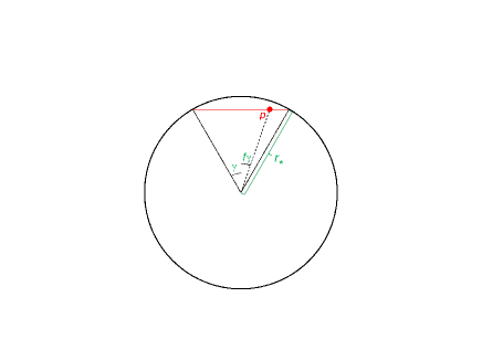
Figure 1: A local operator at $p$, represented by the dot, is on the HRT surface anchored to the boundary of a spherical cap region, $0\leq\psi\leq\gamma$, on the leaf at time $\eta_{*}$, located at $r=r_{*}$. Note that the figure suppresses the time direction; for example, the operator is not at the same time as the leaf.

(The value of $\phi$ is arbitrary because of the symmetry of the problem; below we take $\phi=0$ without loss of generality.) In cylindrical coordinates, this implies that the location of the operator, $(\eta,\xi,z)=(\eta_{B},\xi_{B},z_{B})$, is given by

$$\eta_{B}= \eta_{*}+\frac{\dot{a}}{2a}(\xi_{*}^{2}-\xi_{B}^{2})-\frac{\dot{a}}{16a^{3}}(\xi_{*}^{2}-\xi_{B}^{2})\bigl{\{}4\dot{a}^{2}\xi_{*}^{2}-a\ddot{a}(3\xi_{*}^{2}-\xi_{B}^{2})\bigr{\}},$$ (16)

$$\xi_{B}= \frac{\tan(f\gamma)}{\tan\gamma}\xi_{*},$$ (17)

$$z_{B}= 0,$$ (18)

where we have ignored the terms higher order than $\eta^{(4)}(\xi)$ in Eq. (10), which are not relevant for our leading order calculation. The future light cone associated with $p$ is then given by

$$\eta=\eta_{B}+\sqrt{(x-\xi_{B})^{2}+y^{2}+z^{2}},$$ (19)

where we have introduced the coordinates $x=\xi\cos\phi$ and $y=\xi\sin\phi$.

In order to derive the butterfly velocity for the operator at $p$, we need to find the smallest spherical cap region on the leaf at $\eta=\eta_{*}+\delta\eta$

$$\Gamma^{\prime}:0\leq\psi\leq\gamma+\delta\gamma,$$ (20)

so that the entanglement wedge associated with the complement of $\Gamma^{\prime}$ on the leaf does not contain the interior of the future light cone of $p$, Eq. (19). This occurs for the value of $\delta\gamma$ at which the HRT surface anchored to $\partial\Gamma^{\prime}$

$$\eta(\xi)= \eta_{*}+\frac{\dot{a}}{2a}(\xi_{*}^{2}-\xi^{2})-\frac{\dot{a}}{16a^{3}}(\xi_{*}^{2}-\xi^{2})\bigl{\{}4\dot{a}^{2}\xi_{*}^{2}-a\ddot{a}(3\xi_{*}^{2}-\xi^{2})\bigr{\}}$$

$${}+\delta\eta-\frac{\dot{a}^{2}}{2a^{2}}\biggl{(}1-\frac{a\ddot{a}}{\dot{a}^{2}}\biggr{)}(\xi_{*}^{2}-\xi^{2})\delta\eta$$

$${}+\frac{\dot{a}}{a}\xi_{*}\delta\xi_{*}-\frac{\dot{a}}{4a^{3}}\bigl{\{}2\dot{a}^{2}(2\xi_{*}^{2}-\xi^{2})-a\ddot{a}(3\xi_{*}^{2}-2\xi^{2})\bigr{\}}\xi_{*}\delta\xi_{*},$$ (21)

$$z(\xi)= \biggl{(}1-\frac{a\ddot{a}}{\dot{a}^{2}}\biggr{)}\cos\gamma\,\delta\eta-\frac{a}{\dot{a}}\sin\gamma\,\delta\gamma,$$ (22)

is tangent to the light cone. Here,

$$\delta\xi_{*}=\biggl{(}1-\frac{a\ddot{a}}{\dot{a}^{2}}\biggr{)}\sin\gamma\,\delta\eta+\frac{a}{\dot{a}}\cos\gamma\,\delta\gamma,$$ (23)

and we have suppressed (some of) the terms that do not contribute to the leading order result.

The conditions for the tangency are given by

$$\eta(x) =\eta_{B}+\sqrt{(x-\xi_{B})^{2}+y^{2}+z(x)^{2}},$$ (24)

$$\frac{d\eta(x)}{dx} =\frac{x-\xi_{B}}{\sqrt{(x-\xi_{B})^{2}+y^{2}+z(x)^{2}}},$$ (25)

$$y =0,$$ (26)

where the functions $\eta(x)$ and $z(x)$ are given by Eqs. (21) and (22). These yield the relation between $\delta\eta$ and $\delta\gamma$

$$\delta\eta=\frac{\dot{a}^{2}}{4a^{2}}(3\xi_{*}^{2}-2\xi_{B}^{2})\xi_{*}\delta\gamma,$$ (27)

as well as the location in which the HRT surface touches the light cone

$$x=\xi_{B}-\frac{\dot{a}}{a}\xi_{*}\xi_{B}\delta\gamma.$$ (28)

Using Eq. (17), Eq. (27) becomes

$$\frac{\delta\gamma}{\delta\eta}=\frac{4\dot{a}}{a}\frac{1}{3-2f^{2}}\frac{1}{\gamma^{3}},$$ (29)

where we have used $\xi_{*}=\gamma a/\dot{a}$; see Eqs. (7) and (9). Representing the butterfly velocity $v_{B}$ in terms of the coordinate distance along the holographic space, $\delta\lambda=r_{*}\delta\gamma$, and the conformal time, we finally obtain

$$v_{B}\equiv\frac{\delta\lambda}{\delta\eta}=\frac{4}{3-2f^{2}}\frac{1}{\gamma^{3}}.$$ (30)

There are several features one can see in Eq. (30). First, the butterfly velocity is non-negative, $v_{B}\geq 0$, as expected. Second, for $\gamma\ll 1$, which we are focusing on here, the butterfly velocity is much faster than the speed of light. In fact, it diverges as $\gamma\rightarrow 0$ with the specific power of $\gamma^{-3}$. When the operator is at the tip of the HRT surface, i.e. $f=0$, the butterfly velocity takes the particularly simple form

$$v_{B}|_{f=0}=\frac{4}{3}\frac{1}{\gamma^{3}}.$$ (31)

In Fig. 2, we plot $v_{B}\gamma^{3}$ as a function of $f$.

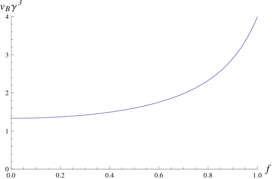
Figure 2: Butterfly velocity $v_{B}$ multiplied by $\gamma^{3}$ as a function of $f$. Here, $\gamma$ is the angular size of the leaf region, and $f$ is the fractional displacement of the bulk local operator from the tip of the HRT surface; see Eq. (15).

We find that the butterfly velocity increases as the operator moves closer to the holographic screen:

$$\frac{dv_{B}}{df}=\frac{16f}{(3-2f^{2})^{2}}\frac{1}{\gamma^{3}}>0.$$ (32)

This is consistent with the monotonicity result in Ref. [8].

It is interesting that the scale factor has completely dropped out from the final expression of Eq. (30). This implies that regardless of the content of the universe, the short distance behavior of the butterfly velocity is universal in the holographic theory of flat FRW spacetimes. As we will see in the next subsection, the butterfly velocity’s dependence on the scale factor appears as we move away from the $\gamma\ll 1$ limit. This suggests that the details of the FRW bulk physics are related with long distance effects in the holographic theory.

3.2 Local operators at arbitrary depths

Beyond the $\gamma\ll 1$ limit, we must resort to a numerical method in order to solve for the butterfly velocity. For this purpose, we focus on the case in which the universe is dominated by a single ideal fluid component with the equation of state parameter $w$. In this case, the scale factor behaves as

$$a(\eta)\propto\left\{\begin{array}[]{l}\eta^{\frac{2}{1+3w}}\\ e^{c\eta}\,\,(c>0)\end{array}\right.\quad\mbox{for}\quad\eta\,\left\{\!\begin{array}[]{l}\neq-\frac{1}{3}\\ =-\frac{1}{3}\end{array}.\right.$$ (33)

When the universe is dominated by a single fluid component, the butterfly velocity $v_{B}$, expressed in terms of angle $\gamma$, does not depend on time $\eta$. This can be seen by using appropriate coordinate transformations, in a way analogous to the argument in Section III A 1 of Ref. [11] showing that a screen entanglement entropy normalized by the leaf area does not depend on time.

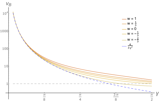
Figure 3: Butterfly velocity $v_{B}$ of a bulk local operator at the tip of the HRT surface, $f=0$, as a function of the angular size $\gamma$ of the leaf region for $w=1$, $1/3$, $0$, $-1/3$, and $-2/3$ (solid curves, from top to bottom). The dashed curve represents $v_{B}=4/3\gamma^{3}$, the analytic result obtained for $\gamma\ll 1$ in Eq. (31). The horizontal dashed line represents the speed of light.

In Fig. 3, we show the results of our numerical calculations of the butterfly velocity, $v_{B}$, as a function of $\gamma$ for a bulk operator located on the tip of the HRT surface, $f=0$, for $w=1$, $1/3$, $0$, $-1/3$, and $-2/3$. We find that beyond $\gamma\ll 1$, the butterfly velocity deviates from the limiting expression of Eq. (31), which is depicted by the dashed curve. In fact, the functional form of $v_{B}|_{f=0}(\gamma)$ is not universal and depends on $w$.

We find that for sufficiently large values of $w$ the butterfly velocity $v_{B}|_{f=0}$ is always faster than the speed of light (depicted by the horizontal dashed line), while for smaller values of $w$ it can be slower than the speed of light for $\gamma$ close to $\pi/2$ (i.e. when the subregion on the leaf becomes large, approaching a hemisphere). The boundary between the two behaviors lies at $w=-1/3$, when the expansion of the universe changes between deceleration and acceleration.

3.3 Arbitrary spacetime dimensions

There is no obstacle in performing the same calculations as in the previous subsections in arbitrary spacetime dimensions. Here we present the analytic results corresponding to those in Section 3.1 for $(d+1)$-dimensional flat FRW universes.

The butterfly velocity, corresponding to Eq. (30), is given by

$$v_{B}=\frac{2}{\frac{d+3}{d+1}-f^{2}}\frac{1}{\gamma^{3}}.$$ (34)

Again, this is non-negative and does not depend on the scale factor. We also find that the exponent of $\gamma$ is universal

$$v_{B}\sim\frac{1}{\gamma^{3}},$$ (35)

regardless of the spacetime dimension. The $f$ dependence of $v_{B}$ is given by

$$\frac{dv_{B}}{df}=\frac{4f}{\bigl{(}\frac{d+3}{d+1}-f^{2}\bigr{)}^{2}}\frac{1}{\gamma^{3}}>0,$$ (36)

which is consistent with the monotonicity result of Ref. [8].

4 Discussion

Our investigation has used a definition of butterfly velocity that differs from that in the literature regarding lattice systems and spin chains. The main difference is that in our case, the excitations of concern (in the boundary theory) are not local operators. They have support on a large subregion of the space. This is in contrast to the lattice definition which considers commutators of local operators separated in space and time. But the conceptual overlap is clear; we are concerned with when and where operators commute. The investigation of this paper allows us to find the effective “light cone” in the holographic theory.

Sending $\gamma\rightarrow 0$ would correspond to a local operator in the holographic theory, and the result that the butterfly velocity diverges in this limit may seem to indicate that the holographic theory is highly nonlocal. However, this is not necessarily the case, as the divergent velocity is integrable. By setting $f=0$ in Eq. (34) and converting $\lambda$ to $\gamma$ (see, e.g., Eqs. (29) and (30)), we obtain

$$\frac{d\gamma}{d\eta}=\frac{q_{d}}{\eta}\frac{2(d+1)}{(d+3)\gamma^{3}},$$ (37)

where $q_{d}=2/(d-2+dw)$. From this expression, we find

$$\gamma(t_{\rm H})=\left[\frac{8(d+1)}{d+3}t_{\rm H}\right]^{\frac{1}{4}},$$ (38)

where $t_{\rm H}=q_{d}\ln(\eta/\eta_{i})$, the number of Hubble times elapsed since the excitation. This shows that the light cone spreads like $t^{1/4}$, regardless of dimension.

Sub-linear growth like this is not an uncommon phenomenon in physics. A localized heat source subject to the heat equation will diffuse as $t^{1/2}$. Even spin chain systems where the Lieb-Robinson bound applies (and suggests a linear dispersion) can admit power law behavior for the effective growth of operators [26]. The specific relationship of $\varDelta x\sim\varDelta t^{1/4}$ suggests that we should be looking for a theory with dynamical exponent $z=4$, and the fact that this holds regardless of spacetime dimension may indicate that a Lifshitz field theory with $z=4$ is the appropriate dual theory for flat FRW spacetimes. Note that results from Ref. [8] show that $v_{B}\rightarrow 1$ as $\gamma\rightarrow 0$ for asymptotically AdS spacetimes. Similarly analyzing this result would suggest that a $z=1$ theory is the appropriate dual for AdS, as is indeed the case. These ideas will be investigated in future work.

References

- [1] G. ’t Hooft, “Dimensional reduction in quantum gravity,” in Salamfestschrift, edited by A. Ali, J. Ellis, and S. Randjbar-Daemi (World Scientific, Singapore, 1994), p. 284 [gr-qc/9310026].
- [2] L. Susskind, “The world as a hologram,” J. Math. Phys. 36, 6377 (1995) [hep-th/9409089].
- [3] R. Bousso, “The holographic principle,” Rev. Mod. Phys. 74, 825 (2002) [hep-th/0203101].
- [4] J. Maldacena, “The large N limit of superconformal field theories and supergravity,” Int. J. Theor. Phys. 38, 1113 (1999) [Adv. Theor. Math. Phys. 2, 231 (1998)] [hep-th/9711200].
- [5] S. H. Shenker and D. Stanford, “Black holes and the butterfly effect,” JHEP 03, 067 (2014) [arXiv:1306.0622 [hep-th]].
- [6] D. A. Roberts, D. Stanford and L. Susskind, “Localized shocks,” JHEP 03, 051 (2015) [arXiv:1409.8180 [hep-th]].
- [7] D. A. Roberts and B. Swingle, “Lieb-Robinson bound and the butterfly effect in quantum field theories,” Phys. Rev. Lett. 117, 091602 (2016) [arXiv:1603.09298 [hep-th]].
- [8] X.-L. Qi and Z. Yang, “Butterfly velocity and bulk causal structure,” arXiv:1705.01728 [hep-th].
- [9] A. Almheiri, X. Dong and D. Harlow, “Bulk locality and quantum error correction in AdS/CFT,” JHEP 04, 163 (2015) [arXiv:1411.7041 [hep-th]].
- [10] F. Pastawski, B. Yoshida, D. Harlow and J. Preskill, “Holographic quantum error-correcting codes: toy models for the bulk/boundary correspondence,” JHEP 06, 149 (2015) [arXiv:1503.06237 [hep-th]].
- [11] Y. Nomura, N. Salzetta, F. Sanches and S. J. Weinberg, “Toward a holographic theory for general spacetimes,” Phys. Rev. D 95, 086002 (2017) [arXiv:1611.02702 [hep-th]].
- [12] Y. Nomura, P. Rath and N. Salzetta, “Classical spacetimes as amplified information in holographic quantum theories,” arXiv:1705.06283 [hep-th].
- [13] R. Bousso and N. Engelhardt, “New area law in general relativity,” Phys. Rev. Lett. 115, 081301 (2015) [arXiv:1504.07627 [hep-th]].
- [14] R. Bousso and N. Engelhardt, “Proof of a new area law in general relativity,” Phys. Rev. D 92, 044031 (2015) [arXiv:1504.07660 [gr-qc]].
- [15] F. Sanches and S. J. Weinberg, “Refinement of the Bousso-Engelhardt area law,” Phys. Rev. D 94, 021502 (2016) [arXiv:1604.04919 [hep-th]].
- [16] F. Sanches and S. J. Weinberg, “A holographic entanglement entropy conjecture for general spacetimes,” Phys. Rev. D 94, 084034 (2016) [arXiv:1603.05250 [hep-th]].
- [17] R. Bousso, “Holography in general space-times,” JHEP 06, 028 (1999) [hep-th/9906022].
- [18] A. Hamilton, D. N. Kabat, G. Lifschytz and D. A. Lowe, “Holographic representation of local bulk operators,” Phys. Rev. D 74, 066009 (2006) [hep-th/0606141].
- [19] B. Czech, J. L. Karczmarek, F. Nogueira and M. Van Raamsdonk, “The gravity dual of a density matrix,” Class. Quant. Grav. 29, 155009 (2012) [arXiv:1204.1330 [hep-th]].
- [20] X. Dong, D. Harlow and A. C. Wall, “Reconstruction of bulk operators within the entanglement wedge in gauge-gravity duality,” Phys. Rev. Lett. 117, 021601 (2016) [arXiv:1601.05416 [hep-th]].
- [21] V. E. Hubeny, M. Rangamani and T. Takayanagi, “A covariant holographic entanglement entropy proposal,” JHEP 07, 062 (2007) [arXiv:0705.0016 [hep-th]].
- [22] P. Hayden, S. Nezami, X.-L. Qi, N. Thomas, M. Walter and Z. Yang, “Holographic duality from random tensor networks,” JHEP 11, 009 (2016) [arXiv:1601.01694 [hep-th]].
- [23] T. Faulkner and A. Lewkowycz, “Bulk locality from modular flow,” JHEP 07, 151 (2017) [arXiv:1704.05464 [hep-th]].
- [24] J. Cotler, P. Hayden, G. Salton, B. Swingle and M. Walter, “Entanglement wedge reconstruction via universal recovery channels,” arXiv:1704.05839 [hep-th].
- [25] F. Sanches and S. J. Weinberg, “Boundary dual of bulk local operators,” Phys. Rev. D 96, 026004 (2017) [arXiv:1703.07780 [hep-th]].
- [26] D. J. Luitz and Y. Bar Lev, “Information propagation in isolated quantum systems,” Phys. Rev. B 96, 020406 (2017) [arXiv:1702.03929 [cond-mat.dis-nn]].