Strategy Synthesis in POMDPs
via Game-Based Abstractions

Abstract

We study synthesis problems with constraints in partially observable Markov decision processes (POMDPs), where the objective is to compute a strategy for an agent that is guaranteed to satisfy certain safety and performance specifications. Verification and strategy synthesis for POMDPs are, however, computationally intractable in general. We alleviate this difficulty by focusing on planning applications and exploiting typical structural properties of such scenarios; for instance, we assume that the agent has the ability to observe its own position inside an environment. We propose an abstraction refinement framework which turns such a POMDP model into a (fully observable) probabilistic two-player game (PG). For the obtained PGs, efficient verification and synthesis tools allow to determine strategies with optimal safety and performance measures, which approximate optimal schedulers on the POMDP. If the approximation is too coarse to satisfy the given specifications, an refinement scheme improves the computed strategies. As a running example, we use planning problems where an agent moves inside an environment with randomly moving obstacles and restricted observability. We demonstrate that the proposed method advances the state of the art by solving problems several orders-of-magnitude larger than those that can be handled by existing POMDP solvers. Furthermore, this method gives guarantees on safety constraints, which is not supported by the majority of the existing solvers.

I Introduction

Partially observable Markov decision processes (POMDPs) are the formalism of choice to model environments where the current state is not perfectly known [1, 2, 3]. They extend Markov decision processes (MDPs), which are non-deterministic models in which an agent chooses to perform an action under full knowledge of the environment in which it operates. The outcome of that action is a probability distribution over the successor states. In contrast, in a POMDP the agent cannot directly assess the state of the system, but has only access to observations. By tracking the observations, an agent can infer the likelihood of the environment (and itself) being in a particular state. This likelihood is called the belief state of the agent. Upon executing an action, the agent updates the belief state according to new observations. The belief state together with an update function forms a (possibly infinite) MDP, commonly referred to as the underlying belief MDP [4]. For finite MDPs, tools like PRISM [5] or Storm [6] employ efficient model checking algorithms to assess the probability to reach a certain set of states. However, due to the potentially infinite belief space, POMDP verification is in general undecidable [7] and also intractable even for rather small instances, and the synthesis of strategies with any given constraints can become a real challenge.

POMDPs are used in a multitude of applications, including control [3], scheduling [8], reinforcement learning [9], and planning [1]. In this paper, we restrict ourselves to POMDPs describing typical planning scenarios, although it is not unlikely that similar structures may exist in scenarios from many other applications as well. This restriction allows to exploit certain structural properties, resulting in significantly improved scalability compared to general POMDP solution approaches. One scenario we are especially interested in is offline planning in dynamically changing environments with uncertainties. Here, the goal is to find a strategy for an agent that ensures certain desired behavior [10]. As a running example, we take a scenario where a controllable agent needs to traverse a workspace with obstacles that can be both static or randomly moving. The agent has a limited range of view and can observe moving obstacles only if they are close enough and not hidden behind static obstacles. A traversal of the workspace is safe if the agent avoids any collision.

Summary of the proposed approach

Figure 1: Schematic overview of the approach

We outline the approach and the structure of the paper in Fig. 1, and discuss the details in the respective sections. We first encode the problem as a POMDP. Planning scenarios as described above naturally induce certain structural properties in these POMDPs. In particular, we assume that the agent can observe its own state. On the other hand, the state of the environment, e. g., the exact position of the moving obstacles, is observable only if the agent and the obstacle are close according to a given distance metric. We propose an abstraction method that, intuitively, lumps together the states that induce the same observation. Since it is not exactly known in which state of the environment a certain action is executed, a non-deterministic choice over these lumped states is introduced. Resolving this choice induces a new level of non-determinism into the system in addition to the choices of the agent: The POMDP abstraction results in a probabilistic two-player game (PG) [12]. The agent has the role of the first player and chooses an action; the second player determines in which of the possible (concrete) states the action is executed. When verifying whether a desired behavior is possible in this abstraction, model checking computes, as a byproduct, an optimal strategy for the agent on this PG with regard to that behavior.

This automated abstraction procedure is inspired by game-based abstraction [12, 13, 14] of potentially infinite MDPs, where states are lumped in a similar fashion. As quantitative reachability problems are undecidable for POMDPs [7], our approach is necessarily incomplete, as it does not always obtain a strategy that yields the required probability even if one exists. We show that our approach is sound: A strategy for the first player in the PG defines a strategy for the agent in the original POMDP. Guarantees for the strategy carry over to the POMDP, as, for each strategy, the bounds computed in the PG underapproximate the actual bounds in the POMDP.

We also define a scheme to refine the abstraction by considering a history of previous observations. We do this by encoding the last observable position of the moving obstacles into the current state of the game. Having access to the last known position limits the possible current positions of the obstacle, mimicking the belief state of the agent. Consequently, the second player in the abstraction is more restricted, and thus the method obtains tighter bounds on the POMDP. Therefore, the use of history increases the likelihood of satisfying the given specification. We also modify the environment by placing cameras, effectively increasing the number of observable positions.

We developed a Python toolchain, which takes a graph formulation of the workspace as input and implements the proposed abstraction-refinement procedure. The toolchain uses PRISM-games [11] as a model checker for PGs. We created a vast range of examples for the type of planning scenario considered. Our preliminary results indicate an improvement by up to three orders of magnitude over the state of the art in POMDP verification [8].

Contribution

To summarize our work, we present an abstraction-refinement scheme for POMDPs that iteratively abstracts POMDPs into probabilistic two-player games. We show that our approach is not only sound, but for various examples from our domain, yields – within minutes of computation time – strategies whose quality typically matches those obtained by existing POMDP solvers. The method thereby is considerably faster on small models, and scales to significantly larger instances, which could not be analyzed before.

Related Work

General verification problems for POMDPs and their decidability are studied in [15, 7]. A recent survey about decidability results and algorithms for $\omega$-regular properties is given in [16, 17]. The probabilistic model checker PRISM has been extended recently to support POMDPs [8]. Partly based on the methods from [18], it produces lower and upper bounds for a variety of queries. Reachability can be analyzed for POMDPs for up to several tens of thousands of states. An overview on point-based value iteration algorithms for analyzing POMDPs is given in [4]. In [19], iterative refinement is proposed to solve POMDPs: Starting with total information, strategies that depend on unobservable information are excluded.

In [20], a compositional framework for reasoning about POMDPs is introduced. An abstraction-refinement framework based on counterexamples is considered in [21]. In contrast to our work, neither [20] nor [21] specializes on planning problems, and there is neither an implementation available nor any analysis how well these methods scale to systems of relevant size. Instead of automated abstraction, an interactive human-in-the-loop approach for strategy synthesis in POMDPs is described in [22], but such an approach, in contrast to the method described here, may not be fully automated. The strategies obtained by the method in this paper are finite-memory strategies. Finite-memory strategies for POMDPs have been considered in [23], but the methods based on non-linear programming may not scale to large state spaces (e. g., those on which we demonstrate the proposed method in Sect. V). In contrast, the proposed method utilizes efficient value-iteration-based methods, which are less affected by the size of the state space. The work in [24] studies the relationship between parametric Markov chains (pMCs) and finite-memory strategies for POMDPs; the close connection between the two formalisms allows to adopt algorithms for pMC synthesis for POMDP strategy computation. Finally, an overview of applications for PGs is given in [25].

Several methods have been proposed for POMDPs that appear in the context of motion planning. Sampling-based methods for motion planning in POMDP scenarios are considered in [26, 27, 28, 29]. Other methods employ control techniques to synthesize strategies with safety considerations under noisy observations and dynamics [1, 30, 31]. Preprocessing of POMDPs in motion planning problems for robotics is suggested in [32].

This paper is an extended version of [33], and offers additional details on our theoretical results as well as extended experiments.

II Preliminaries

II-A Probabilistic Games

For a finite or countably infinite set $X$, $\mu\colon X\to[0,1]$ denotes a probability distribution over $X$ if $\sum_{x\in X}\mu(x)=1$; the set of all probability distributions over $X$ is $\mathit{Dist}(X)$. The Dirac distribution $\delta_{x}\in\mathit{Dist}(X)$ on $x\in X$ is given by $\delta_{x}(x)=1$ and $\delta_{x}(y)=0$ for $y\in X\setminus\{x\}$.

Definition 1 (Probabilistic Game)

A probabilistic game (PG) is a tuple $\mathsf{G}=(S_{1},S_{2},s_{\text{init}},\mathit{Act},P)$ where $S=S_{1}\mathbin{\dot{\cup}}S_{2}$ is a finite set of states, $S_{1}$ the set of states of Player 1, $S_{2}$ the set of states of Player 2, $s_{\text{init}}\in S$ the initial state, $\mathit{Act}$ a finite set of actions, and $P\colon S\times\mathit{Act}\mathrel{\ooalign{\hfil$\mapstochar\mkern 5.0mu$\hfil\cr$\to$\cr}}\mathit{Dist}(S)$ a (partial) probabilistic transition function.

Let $\mathit{Act}(s)=\bigl{\{}\alpha\in\mathit{Act}\,\big{|}\,(s,\alpha)\in\operatorname{dom}(P)\bigr{\}}$ denote the available actions in $s\in S$. We assume that PG $\mathsf{G}$ is free of deadlock states, i. e., $\mathit{Act}(s)\neq\emptyset$ for all $s\in S$. A Markov decision process (MDP) $\mathsf{M}$ is a PG with $S_{2}=\emptyset$. We write $\mathsf{M}=(S,s_{\text{init}},\mathit{Act},P)$. A discrete-time Markov chain (MC) is an MDP with $|\mathit{Act}(s)|=1$ for all $s\in S$. We write $\mathsf{C}=(S,s_{\text{init}},P)$ where $P\colon S\mathrel{\ooalign{\hfil$\mapstochar\mkern 5.0mu$\hfil\cr$\to$\cr}}\mathit{Dist}(S)$.

At Player 1 states (i. e., if $s\in S_{1}$) Player 1 chooses an available action $\alpha\in\mathit{Act}(s)$ non-deterministically, if $s\in S_{2}$, Player 2 chooses. The successor state of $s$ is determined probabilistically according to the probability distribution $P(s,\alpha)$: The probability of $s^{\prime}$ being the next state is $P(s,\alpha)(s^{\prime})$. The state of the game is then $s^{\prime}$.

A path through $\mathsf{G}$ is a finite or infinite sequence $\pi=s_{0}\xrightarrow{\alpha_{0}}s_{1}\xrightarrow{\alpha_{1}}\cdots$, where $s_{0}=s_{\text{init}}$, $s_{i}\in S$, $\alpha_{i}\in\mathit{Act}(s_{i})$, and $P(s_{i},\alpha_{i})(s_{i+1})>0$ for all $i\in\mathbb{N}$. The $(i{+}1)$-th state $s_{i}$ on $\pi$ is $\pi(i)$, and $\operatorname{last}(\pi)$ denotes the last state of $\pi$ if $\pi$ is finite. The set of (in)finite paths is $\mathit{Paths}^{\mathrm{fin}}_{\mathsf{G}}$ ($\mathit{Paths}^{\mathrm{inf}}_{\mathsf{G}}$).

To define a probability measure over the paths of a PG $\mathsf{G}$, the non-determinism needs to be resolved by a strategy for each player.

Definition 2 (PG Strategy)

A strategy $\sigma$ for a PG $\mathsf{G}$ is a pair $\sigma=(\sigma_{1},\sigma_{2})$ of functions $\sigma_{i}\colon\{\pi\in\mathit{Paths}^{\mathrm{fin}}_{\mathsf{G}}\mid\operatorname{last}(\pi)\in S_{i}\}\to\mathit{Dist}(\mathit{Act})$ such that for all $\pi\in\mathit{Paths}^{\mathrm{fin}}_{\mathsf{G}}$, $\{\alpha\mid\sigma_{i}(\pi)(\alpha)>0\}\subseteq\mathit{Act}\bigl{(}\operatorname{last}(\pi)\bigr{)}$. We also call $\sigma_{i}$ a Player $i$ strategy. $\Sigma_{\mathsf{G}}$ denotes the set of all strategies of $\mathsf{G}$ and $\Sigma_{\mathsf{G}}^{i}$ all Player $i$ strategies of $\mathsf{G}$.

For MDPs, a strategy consists of a Player 1 strategy only. A Player $i$ strategy $\sigma_{i}$ is memoryless if $\operatorname{last}(\pi)=\operatorname{last}(\pi^{\prime})$ implies $\sigma_{i}(\pi)=\sigma_{i}(\pi^{\prime})$ for all $\pi,\pi^{\prime}\in\operatorname{dom}(\sigma_{i})$. It is deterministic if $\sigma_{i}(\pi)$ is a Dirac distribution for all $\pi\in\operatorname{dom}(\sigma_{i})$. A memoryless deterministic strategy is of the form $\sigma_{i}\colon S_{i}\to\mathit{Act}$.

A strategy $\sigma$ for a PG resolves all non-deterministic choices, yielding an induced MC, for which a probability measure over the set of infinite paths is defined by the standard cylinder set construction [34]. These notions are analogous for MDPs.

II-B Partial Observability

A partially observable Markov decision processes [1] is obtained by restricting the knowledge of the current state of an MPD.

Definition 3 (POMDP)

A partially observable Markov decision process (POMDP) is a tuple $\mathsf{D}=(\mathsf{M},\mathcal{O},\lambda)$ such that $\mathsf{M}=(S,s_{\text{init}},\mathit{Act},P)$ is the underlying MDP of $\mathsf{D}$, $\mathcal{O}$ a finite set of observations, and $\lambda\colon S\to\mathcal{O}$ the observation function.

W. l. o. g. we require that states with the same observations have the same set of enabled actions, i. e., $\lambda(s)=\lambda(s^{\prime})$ implies $\mathit{Act}(s)=\mathit{Act}(s^{\prime})$ for all $s,s^{\prime}\in S$. (Otherwise, since the enabled actions are known to the agent, the states could be distinguished, which contradicts the assumption that the same observations are made in both states.) More general observation functions $\lambda$ have been considered in the literature, taking into account the last action and providing a distribution over $\mathcal{O}$. There is a polynomial transformation of the general case to the POMDP definition used here [17].

The notions of paths and probability measures directly transfer from MDPs to POMDPs. We lift the observation function to paths: For a POMDP $\mathsf{D}$ and a path $\pi=s_{0}\xrightarrow{\alpha_{0}}s_{1}\xrightarrow{\alpha_{1}}\cdots s_{n}\in\mathit{Paths}^{\mathrm{fin}}_{\mathsf{D}}$, the associated observation sequence is $\lambda(\pi)=\lambda(s_{0})\xrightarrow{\alpha_{0}}\lambda(s_{1})\xrightarrow{\alpha_{1}}\cdots\lambda(s_{n})$. Note that several paths in the underlying MDP $\mathsf{M}$ can give rise to the same observation sequence. Strategies have to take this restricted observability into account.

Definition 4 (Observation-Based Strategy)

An observation-based strategy of a POMDP $\mathsf{D}$ is a function $\sigma\colon\mathit{Paths}^{\mathrm{fin}}_{\mathsf{D}}\to\mathit{Dist}(\mathit{Act})$ such that $\sigma$ is a strategy for the underlying MDP and for all paths $\pi,\pi^{\prime}\in\mathit{Paths}^{\mathrm{fin}}_{\mathsf{D}}$ with $\lambda(\pi)=\lambda(\pi^{\prime})$ we have $\sigma(\pi)=\sigma(\pi^{\prime})$. $\Sigma_{\mathsf{D}}^{\mathrm{o}}$ denotes the set of such strategies.

An observation-based strategy selects the next action based on the observations and actions made along the current path.

The semantics of a POMDP can be described using a belief MDP with an uncountable state space. Each state of the belief MDP corresponds to a distribution over the states in the POMDP. This distribution represents the probability of the system to be in any specific state based on the observations made so far. Initially, the belief is a Dirac distribution on the initial state. In general, a POMDP can be defined as having a set of initial states – in this case, the initial belief is a uniform distribution over those states. A formal treatment of belief MDPs is beyond the scope of this paper, for details see [4].

II-C Specifications

Given a set $G\subseteq S$ of goal states and a set $B\subseteq S$ of bad states, we consider quantitative reach-avoid properties of the form $\varphi=\mathbb{P}_{\geqslant p}(\neg B\ \mathcal{U}\ G)$. This specification $\varphi$ is satisfied by a PG if Player 1 has a strategy such that for all strategies of Player 2 the probability is at least $p$ to reach a goal state without entering a bad state in between. For POMDPs, $\varphi$ is satisfied if the agent has an observation-based strategy which leads to a probability of at least $p$ to satisfy $\neg B\ \mathcal{U}\ G$.

For MDPs and PGs, memoryless deterministic strategies suffice to prove or disprove satisfaction of such specifications [35]. For POMDPs, observation-based strategies in their full generality are necessary [36].

III Methodology

We intuitively describe the problem and list the assumptions we make. After formalizing the setting, we present a formal problem statement. We explain the intuition behind the concept of game-based abstraction for MDPs, how to apply it to POMDPs, and prove the correctness of our method.

III-A The Problem

We consider a planning problem that involves $n{+}1$ moving agents inside a world such as a landscape or a room. One agent is controllable (Agent $0$), the other agents (also called obstacles) move probabilistically according to a fixed randomized strategy, which is based on their own location and the location of Agent $0$. We assume that all agents take turns, moving one after another in a fixed order. The position of an agent defines the location inside the world as well as additional properties such as the agent’s orientation. A graph captures all possible movements of an agent between positions, referred to as the world graph of an agent. The nodes in the graph uniquely refer to positions while multiple nodes may refer to the same location in the world. We require that the graph is free of deadlocks: For every position, there is at least one edge in the graph corresponding to a possible action an agent can execute.

A collision occurs, if Agent $0$ shares its location with another agent. The set of goal nodes (goal positions) in the graph is uniquely defined by a set of goal locations in the world. The target is to move Agent $0$ towards a goal node without colliding with other agents. Technically, we need to synthesize a strategy for Agent $0$ that maximizes the probability to achieve the target. Additionally, we make the following assumptions:

• The strategies of all obstacles are known to Agent $0$.

• Agent $0$ is able to observe its own position and knows the goal positions it has to reach.

• The positions of obstacles are observable for Agent $0$ from its current position, if they are visible with respect to a certain distance metric.

Generalizations of the problem statement are discussed in Sect. VI.

III-B Formal Setting

We first define an individual world graph for each Agent $i$ with $0\leq i\leq n$ over a fixed set $\mathit{Loc}$ of locations.

Definition 5 (World Graph of Agent $i$)

The world graph $G_{i}$ for Agent $i$ over $\mathit{Loc}$ is a tuple $G_{i}=(V_{i},v_{i}^{0},\mathit{Mov}_{i},\allowbreak E_{i},\ell_{i})$ such that $V_{i}$ is the set of positions and $v_{i}^{0}\in V_{i}$ is the initial position of Agent $i$. $\mathit{Mov}_{i}$ is the set of movements; the edges $E_{i}\colon V_{i}\times\mathit{Mov}_{i}\mathrel{\ooalign{\hfil$\mapstochar\mkern 5.0mu$\hfil\cr$\to$\cr}}V_{i}$ are the movement effects. The function $\ell_{i}\colon V_{i}\to\mathit{Loc}$ maps a position to the corresponding location.

(a) World graph for Agent 0

(b) World graph for Agent 1 under a randomized strategy $\sigma_{1}$

Figure 2: World graphs for two agents and three positions $s_{1}$, $s_{2}$ and $s_{3}$.

The enabled movements for Agent $i$ in position $v$ are $\mathit{Mov}_{i}(v)=\bigl{\{}m\,\big{|}\,(v,m)\in\operatorname{dom}(E_{i})\bigr{\}}$.

The viewing range of Agent $0$ can be restricted by using a function $\nu_{0}\colon V_{0}\to 2^{\mathit{Loc}}$ which assigns to each position of Agent $0$ the set of visible locations. According to our assumptions, for all $v\in V_{0}$ it holds that $\ell_{0}(v)\in\nu_{0}(v)$ and $\mathit{Mov}_{i}(v)\neq\emptyset$.

Each Agent $i$ with $i>0$ has a randomized strategy $\sigma_{i}\colon V_{0}\times V_{i}\rightarrow\mathit{Dist}(\mathit{Mov}_{i})$, which maps positions of Agent $0$ and Agent $i$ to a distribution over enabled movements of Agent $i$.

Remark 1

It is also possible to allow movements with probabilistic effects in the world graph, e. g., to model uncertainty in the behavior of the agents. As this extension is straightforward, we keep the notations simpler and refrain from allowing probabilistic movements.

Example 1

Fig. 2 visualizes the concept of world graphs for Agent $0$ and one additional agent. For the sake of simplicity, we assume in our examples that locations and positions of the agents coincide – we do not use additional information like the orientation of the agents. Both agents move over the same three locations, but their possible movements over these locations are different. Agent $0$ (Fig. 2a) has two enabled movements in each location, so it can move from one location to either of the other two, but not stay in the same location. For Agent $1$ (Fig. 2b), a randomized strategy has already been applied to the world graph. Positions $s_{1}$ and $s_{3}$, which actually have two enabled movements each, end up with one probabilistic movement instead, while $s_{2}$ only has one enabled movement to begin with. While position $s_{2}$ has only $s_{3}$ as a successor, both $s_{2}$ and $s_{3}$ can be reached with equal probability from $s_{1}$; for $s_{3}$, the probability is higher to move to $s_{1}$ than to stay in $s_{3}$.

As Agent $0$ has restricted vision, not all parts of the world are observable. Therefore, the world graphs for all agents – with randomized strategies for the obstacles – are ultimately subsumed by a single world POMDP which has an underlying world MDP. The MDP models the possible behaviors of all agents based on their associated world graphs.

Definition 6 (World MDP)

For world graphs $G_{0},\ldots,G_{n}$ and strategies $\sigma_{1},\ldots,\sigma_{n}$, the induced world MDP $\mathsf{M}=(S,s_{\text{init}},\mathit{Act},P)$ is defined by $S=V_{0}\times V_{1}\times\cdots\times V_{n}\times\{0,\ldots,n\}$, $s_{\text{init}}=(v_{0}^{0},v_{1}^{0},\ldots,v_{n}^{0},0)$, and $\mathit{Act}=\mathit{Mov}_{0}\mathbin{\dot{\cup}}\{\bot\}$. $P$ is defined by:

• For $\alpha\in\mathit{Mov}_{0}(v_{0})$ and $\breve{v}\in V_{1}\times\cdots\times V_{n}$, we have $P\bigl{(}(v_{0},\breve{v},0),\alpha\bigr{)}=\delta_{(E_{0}(v_{0},\alpha),\breve{v},1)}$.

• $P\bigl{(}(v_{0},\hat{v},v_{i},\breve{v},i),\bot\bigr{)}\bigl{(}(v_{0},\hat{v},v^{\prime}_{i},\breve{v},i{+}1\mod n{+}1)\bigr{)}=q$, with $\hat{v}\in V_{1}\times\cdots\times V_{i-1}$, $\breve{v}\in V_{i+1}\times\cdots\times V_{n}$, $1\leq i\leq n$ and $q=\sum_{\{m\,|\,E_{i}(v_{i},m)=v^{\prime}_{i}\}}\sigma_{i}(v_{0},v_{i})(m)$.

• $0$ in all other cases.

Figure 3: Cut-out of the world MDP for the world graphs from Fig. 2

The first item in the definition of $P$ translates each movement in the world graph of Agent $0$ into an action in the MDP that connects states with probability one, i. e., a Dirac distribution is attached to each action. Upon taking the action, the position of Agent $0$ changes and Agent $1$ has to move next.

The second item defines movements of the obstacles. In each state where Agent $i$ (with $i>0$) is moving next, the action $\bot$ reflecting this move is added. The outcome of $\bot$ is determined by $\sigma_{i}$ and by Agent $i{+}1$ moving next.

Example 2

Fig. 3 shows a cut-out of the world MDP built from the world graphs in Fig. 2a and 2b. The full world MDP contains 18 different states. The first two numbers in each state identify the current positions of Agent $0$ and Agent $1$, respectively; the third entry, the turn indicator, states which agent moves next. Agent $1$ moves in a purely probabilistic manner according to its strategy $\sigma_{1}$, whereas Agent $0$ can chose between two different actions, $+$ and $-$. Each agent’s movements only change its own position as well as the turn indicator.

Definition 7 (World POMDP)

Let $\mathsf{M}$ be a world MDP. The world POMDP $\mathsf{D}=(\mathsf{M},\mathcal{O},\lambda)$ is defined by $\mathcal{O}=V_{0}\times\bigtimes_{1\leq i\leq n}(V_{i}\mathbin{\dot{\cup}}\{\mp\})$ and $\lambda$ as follows:

$$\lambda((v_{0},\ldots,v_{n}))_{i}=\begin{cases}v_{i},&\text{if $\ell(v_{i})\in\nu_{0}(v_{0})$},\\ \mp,&\text{otherwise.}\end{cases}$$

The position of Agent $i$ is observed if and only if the location of Agent $i$ is visible from the position of Agent $0$. The reason is that $\ell(v_{i})$ describes the location corresponding to the current position of Agent $i$, and $\nu_{0}(v_{0})$ is the set of locations visible from the current position of Agent $0$. If the location of Agent $i$ is not visible, a value $\mp$, which is referred to as far away, is observed.

Figure 4: World POMDP corresponding to Fig. 3

Example 3

Fig. 4 shows the world POMDP corresponding to the world MDP in Fig. 3, assuming that Agent $0$ can only observe the position of Agent $1$ when both agents share a location. As soon as Agent $1$ moves to a different location, it is observed as $\mp$. For instance, $(3,1,0)$ and $(3,2,0)$ are still distinct states as far as traces in the POMDP are concerned, but as Agent $0$ can no longer distinguish between the two, it has to behave the same in both states, and we aggregate these states under the same observation label $(3,\mp,0)$.

Given a set $\textsl{GoalLocations}\subseteq\mathit{Loc}$, the mappings $\ell_{i}\colon V_{i}\to\mathit{Loc}$ are used to define the states corresponding to collisions and goal locations. In particular, we have $\textsl{Collision}=\bigl{\{}((v_{0},\ldots,v_{n}),j)\in S\,\big{|}\,\exists 1\leq i\leq n.\,\ell_{0}(v_{0})=\ell_{i}(v_{i})\bigr{\}}$ and $\textsl{Goals}=\bigl{\{}((v_{0},\ldots,v_{n}),j)\,\big{|}\,\ell_{0}(v_{0})\in\textsl{GoalLocations}\bigr{\}}$.

Formal Problem Statement

We assume that we are given (1) a safety threshold $p\in[0,1]$, (2) a world POMDP $\mathsf{D}$ over a set of world graphs $G_{0},\ldots,G_{n}$, (3) a set of collision states Collision, and (4) a set of goal states Goals. We define an observation-based strategy $\sigma\in\Sigma_{\mathsf{D}}^{\mathrm{o}}$ for $\mathsf{D}$ to be $p$-safe for $p\in[0,1]$ if $\mathbb{P}^{\sigma}_{\geqslant p}(\neg\textsl{Collision}\ \mathcal{U}\ \textsl{Goals})$ holds. The goal is to compute a $p$-safe strategy if one exists.

III-C Abstraction

We propose an abstraction method for world POMDPs that builds on game-based abstraction (GBAR), originally defined for MDPs [12, 13].

GBAR for MDPs

For an MDP $\mathsf{M}=(S,s_{\text{init}},\mathit{Act},P)$, we assume a partition $\Pi=\{B_{1},\ldots,B_{k}\}$ of $S$, i. e., a set of non-empty, pairwise disjoint subsets (called blocks) $B_{i}\subseteq S$ with $\bigcup_{i=1}^{k}B_{i}=S$. GBAR takes the partition $\Pi$ and turns each block into an abstract state $B_{i}$; these blocks form the Player 1 states. Then $\mathit{Act}(B_{i})=\bigcup_{s\in B_{i}}\mathit{Act}(s)$. To determine the outcome of selecting $\alpha\in\mathit{Act}(B_{i})$, we add intermediate selector-states $\langle B_{i},\alpha\rangle$ as Player 2 states. In the selector state $\langle B_{i},\alpha\rangle$, emanating actions reflect the choice of the actual state the system is in at $B_{i}$, i. e., $\mathit{Act}\bigl{(}\langle B_{i},\alpha\rangle\bigr{)}=\{s\in B_{i}\,|\,\alpha\in\mathit{Act}(s)\}$. For taking an action $s\in B_{i}$ in $\langle B_{i},\alpha\rangle$, the distribution $P(s,\alpha)$ is lifted to a distribution over abstract states:

$$P\bigl{(}\langle B_{i},\alpha\rangle,s\bigr{)}\bigl{(}B_{j}\bigr{)}=\sum_{s^{\prime}\in B_{j}}P(s,\alpha)(s^{\prime}).$$

The semantics of this PG is as follows: For an abstract state $B_{i}$, Player 1 (controllable) selects an action to execute. In selector states, Player 2 (adversary) selects the worst-case state from $B_{i}$ where the selection was executed.

GBAR for POMDPs

The key idea in GBAR for POMDPs is to merge states with equal observations.

Definition 8 (Abstract PG)

The abstract PG of POMDP $\mathsf{D}=\bigl{(}(S,s_{\text{init}},\mathit{Act},P),\mathcal{O},\lambda\bigr{)}$ is $\mathsf{G}=(S_{1},S_{2},s_{\text{init}}^{\prime},\mathit{Act}^{\prime},P^{\prime})$ with $S_{1}=\bigl{\{}\{s\in S\,|\,\lambda(s)=\lambda(s^{\prime})\}\,\big{|}\,s^{\prime}\in S\bigr{\}}$, $S_{2}=\bigl{\{}\langle B,\alpha\rangle\,\big{|}\,B\in S_{1}\land\alpha\in\mathit{Act}(B)\bigr{\}}$, $s_{\text{init}}^{\prime}=B$ s. t. $s_{\text{init}}\in B$, and $\mathit{Act}^{\prime}=S\mathbin{\dot{\cup}}\mathit{Act}$.

The transition probabilities $P^{\prime}$ are defined as follows:

• $P^{\prime}(B,\alpha)=\delta_{\langle B,\alpha\rangle}$ for $B\in S_{1}$ and $\alpha\in\mathit{Act}(B)$,

• $P^{\prime}\bigl{(}\langle B,\alpha\rangle,s\bigr{)}\bigl{(}B^{\prime}\bigr{)}=\sum_{s^{\prime}\in B^{\prime}}P(s,\alpha)(s^{\prime})$ for $\langle B,\alpha\rangle\in S_{2}$, $s\in B$, and $B^{\prime}\in S_{1}$,

• and $0$ in all other cases.

Figure 5: Abstract world PG corresponding to the world POMDP in Fig. 4. Ellipses denote the states of Player 1, rectangles those of Player 2.

By construction, Player 1 has to select the same action for all states in an abstract state. As the abstract states coincide with the observations, we obtain an observation-based strategy for the POMDP. For the classes of specifications we consider, a memoryless deterministic strategy suffices for PGs to achieve the maximal probability of reaching a goal state without collision [35]. We thus obtain an optimal strategy $\sigma_{1}\colon S_{1}\rightarrow\mathit{Act}$ for Player 1 in the PG which maps every abstract state to an action. As abstract states are constructed such that they coincide with all possible observations in the POMDP (see Def. 8), $\sigma$ maps every observation to an action.

Abstract World PG

We now connect the abstraction to our setting. For the rest of the section, we assume – for the ease of representation – that there is only one uncontrollable agent, i. e., we have Agent $0$ and Agent $1$. Therefore, if Agent $0$ sees an agent and moves, no additional agent will appear. Moreover, Agent $0$ either knows the exact state, or does not know where Agent $1$ is.

We call the abstract PG of the world POMDP the abstract world PG. The abstract states $B_{k}$ in the world PG are either of the form $B_{k}=(v_{0},v_{1},i)$ or of the form $B_{k}=(v_{0},\mp,i)$, with $i\in\{0,1\}$. In the former, Agent $1$ is visible and Agent $0$ has full knowledge, in the latter only the own position is known. Recall that $\mp$ is a specific value for the distance referred to as far away. Furthermore, all states in an abstract state correspond to the same position of Agent $0$. For abstract states with full knowledge, there is no non-determinism of Player 2 involved as these states correspond to a single state in the world POMDP.

Example 4

Fig. 5 shows the abstract world PG for our running example from Figs. 2–4. When there is only one action available, we omit the non-deterministic choice. In $(3,\mp,0)$, Player 1 chooses either $+$ or $-$, leading to $(3,\mp,0,+)$ or $(3,\mp,0,-)$, respectively. Then, Player 2 resolves the far away state to the actual location $1$ or $2$, choosing the successor state corresponding to the resolved far away state and the action chosen by Player 1.

We extend the notion of $p$-safety to strategies in PGs:

Definition 9 ($p$-safe strategy)

A Player 1 strategy $\sigma_{1}\colon S_{1}\rightarrow\mathit{Act}$ is $p$-safe for $p\in[0,1]$ if $\mathbb{P}^{(\sigma_{1},\sigma_{2})}_{\geqslant p}(\neg\textsl{Collision}\ \mathcal{U}\ \textsl{Goals})$ holds for every Player 2 strategy $\sigma_{2}\colon S_{2}\rightarrow\mathit{Act}$.

We formally state the following relationship between strategies in the PG and in the POMDP:

Definition 10

For each memoryless Player 1 strategy $\sigma^{\prime}$ in the abstract world PG, we define a corresponding observation-based strategy $\sigma$ in the POMDP by setting $\sigma(o)=\sigma^{\prime}(B)$ where $o=\lambda(s)$ for all $s\in B$.

Proposition 1

For every path $\pi$ in an abstract world PG under strategy $\sigma^{\prime}$ with $\pi\models(\neg\textsl{Collision}\ \mathcal{U}\ \textsl{Goals})$, there exists a path $\pi^{\prime}$ in the world POMDP with $\pi^{\prime}\models(\neg\textsl{Collision}\ \mathcal{U}\ \textsl{Goals})$.

Consider the following intuitive relation between two paths: Let $B_{0}\xrightarrow{\alpha_{0}}\langle B_{0},\alpha_{0}\rangle\xrightarrow{s\in B_{0}}B_{1}\xrightarrow{\alpha_{1}}\ldots B_{n}$ be a path in the PG. This path is projected to the blocks: $B_{0}\xrightarrow{\alpha_{0}}B_{1}\xrightarrow{\alpha_{1}}\ldots B_{n}$. The location of Agent $0$ encoded in the blocks is independent of the choices made by Player 2. The sequence of actions $\alpha_{0}\alpha_{1}\ldots$ yields a unique path of positions of Agent $0$ in its world graph. Thus, if the path in the PG reaches a goal state, it induces a path in the POMDP which also reaches a goal state. Choices of Player 2 resolve the non-determinism by selecting a concrete position in place of the abstract one. The actual position Agent $1$ inhabits in the POMDP is always one of the options to pick from. Thus, the abstraction over-approximates the probability for Agent $1$ to be in any given location. Lastly, since Agent $0$ can always observe its own location, every collision is observable. Thus if there is a collision in the POMDP, then there is a collision in the PG.

We formalize this relation as a simulation relation as follows: Let $f\colon S\rightarrow S_{1}$ be an abstraction function that maps each state of the world POMDP to an (abstract) Player 1 state in the PG such that $f(s)=f(s^{\prime})$ iff $\lambda(s)=\lambda(s^{\prime})$ for all $s,s^{\prime}\in S$. Then for each transition $s\rightarrow s^{\prime}$ in the POMDP, there is a pair of transitions $f(s)\rightarrow s_{2}\rightarrow f(s^{\prime})$, where $s_{2}\in S_{2}$ is a Player 2 state, in the PG. Fig. 6 shows a graphical representation of this relation.

Theorem 1

Given a $p$-safe strategy in an abstract world PG, the corresponding strategy in the world POMDP is $p^{\prime}$-safe with $p^{\prime}\geq p$.

Proof:

Given a $p$-safe Player 1 strategy $\sigma_{1}$ in the abstract world PG, let $\sigma$ be the corresponding strategy in the POMDP. Applying $\sigma$ to the POMDP resolves all non-determinism and yields an MC. Using the simulation relation established before, we can now compute a Player 2 strategy $\sigma_{2}$ for the PG that resolves the non-determinism in a way such that each transition in the MC is mapped to a 2-step-transition in the PG. The strategy $\sigma_{1}$ is $p$-safe for a given $p\in[0,1]$ if $\mathbb{P}^{(\sigma_{1},\sigma_{2}^{\ast})}_{\geqslant p}(\neg\textsl{Collision}\ \mathcal{U}\ \textsl{Goals})$ holds for every Player 2 strategy $\sigma_{2}^{\ast}$ (according to Def. 9). This property also holds for $\sigma_{2}$ in particular, and as the PG under $\sigma_{1}$ and $\sigma_{2}$ behaves in the same way as the POMDP does under $\sigma$, $\sigma$ is $p^{\prime}$-safe with $p^{\prime}\geq p$. ∎

Figure 6: A graphical representation of the simulation relation.

The assessment of the strategy is conservative: The abstraction allows behavior of the uncontrollable agents that is not possible in the POMDP. These so-called spurious movements are the result of summing up states with the same abstraction: an agent leaving the visible range in one location could re-appear at (jump to) another location far away, if the non-determinism is resolved in another way. Thus, $\sigma_{2}$ does not necessarily represent a worst-case strategy in the PG. Therefore the actual probability of safe traversal might be higher in the POMDP than in the PG.

Applying the strategy to the original POMDP yields a discrete-time Markov chain (MC). This MC can be efficiently analyzed, e. g., by probabilistic model checking to determine the value of $p+\tau$. Naturally, the optimal strategy for the PG needs not be optimal in the POMDP.

If Agent $1$ is visible in a given position, the state of the belief MDP assigns probability $1$ to the corresponding state – the current state of the POMDP is completely observable, and the successor states in the MDP depend solely on the action choice. These beliefs are represented as single states in the abstract world PG. The abstraction lumps for each position of Agent $0$ all (uncountably many) other belief states (in which Agent $1$ is not visible) together.

III-D Refinement of the PG

In the GBAR approach described above, we remove relevant information for an optimal strategy. As described in the previous section, we strengthen (over-approximate) Agent $1$’s behavior by allowing spurious movements.

If, due to this movements, no safe strategy can be found, the abstraction needs to be refined. In GBAR for MDPs [13], abstract states are split heuristically, yielding a finer over-approximation. In our construction, we cannot split abstract states arbitrarily: doing so would destroy the one-to-one correspondence between abstract states and observations as seen in Theorem 1. We would thus obtain a partially observable PG, or equivalently, for a strategy in the PG the corresponding strategy in the original POMDP would be no longer observation-based.

However, we can restrict the spurious movements of Agent $1$ by taking the history of observations made along a path into account. We present three types of history-based refinements.

One-Step History Refinement

If Agent $0$ moves to state $s$ from where Agent $1$ is no longer visible, we have $\lambda(s)=\mp$. Upon the next move, Agent $1$ could thus appear anywhere. However, until Agent $1$ moves, the state of the belief MDP is still Dirac and thus unambiguous; the exact position of Agent $1$ is still known, and thereby the positions where Agent $1$ can appear. Similarly, if Agent $1$ disappears, the state of the belief MDP is also unambiguous, and upon a turn of Agent $0$ in the same direction, Agent $1$ will be visible again.

The (one-step history) refined world PG extends the original PG by additional states $(v_{0},v_{1},i)$ where $v_{1}\not\in\nu_{0}(v_{0})$, i. e., $v_{1}$ is not visible for Agent $0$. These “far away” states are only reached from states with full information. Intuitively, although Agent $1$ is invisible, its position is remembered for one step.

Example 5

Fig. 7 shows the application of one-step history refinement to the Abstract PG from Fig. 5. When Agent $1$ leaves location 3 and is no longer visible, it can only be in location 1. Until Agent $1$ moves, its location is known to Agent $0$.

Figure 7: Abstract world PG with one-step history refinement. Ellipses denote the states of Player 1, rectangles those of Player 2.

Multi-Step History Refinement

Further refinement is possible by considering longer paths. If we first observe Agent $1$ at location $x$, then loose visibility for one turn, and then observe Agent $1$ again at position $y$, then we know that either $x$ and $y$ are at most two moves apart or that such a movement is spurious. To encode the observational history into the states of the abstraction, we store the last known position of Agent $1$, as well as the number $m$ of moves made since then. We then only allow Agent $1$ to appear in positions which are at most $m$ moves away from the last known position. We can cap $m$ by the diameter of the graph.

Region-Based Multi-Step History Refinement

As the refinement above blows up the state space drastically, we utilize magnifying lens abstraction [37]. Instead of single locations, we define regions of locations together with the information if Agent $1$ could be present. After each move, we extend the possible regions by all neighbor regions.

More formally, the (multi-step history) refined world PG has a refined far-away value $\mp$: Given a partition of the positions of Agent $1$, e. g., extracted from the graph, into sets $\mathcal{X}=\{X_{1},\ldots,X_{l}\}$ with $\bigcup_{X\in\mathcal{X}}=V_{1}$ and $X_{i}\cap X_{j}=\emptyset$ for all $1\leq i<j\leq l$. We define $\mp^{\prime}\colon\mathcal{X}\rightarrow\{0,1\}$. Abstract states now are either of the form $(v_{0},v_{1},i)$ as before, or $(v_{0},\mp^{\prime},i)$. For singleton regions, this refinement approach coincides with the method above. The region-based approach also offers some flexibility: If for instance two regions are connected only by the visible area, Agent $0$ can assure whether Agent $1$ enters the other region.

Theorem 2

A $p$-safe strategy in a refined abstract world PG has a corresponding $p$-safe strategy in the world POMDP.

Proof:

First, a deterministic memoryless strategy $\sigma^{\prime}$ on a refined abstract world PG needs to be translated to a strategy $\sigma$ for the original POMDP such that $p$-safety is conserved. Again, we can show a projection of a path $B_{0}\xrightarrow{\alpha_{0}}\langle B_{0},\alpha_{0}\rangle\xrightarrow{s\in B_{0}}B_{1}\xrightarrow{\alpha_{1}}\ldots B_{n}$ in the PG to the blocks $B_{0}\xrightarrow{\alpha_{0}}B_{1}\xrightarrow{\alpha_{1}}\ldots B_{n}$, and again, the location of Agent $0$ is independent of the choices Player 2 makes. However, each block on the path no longer corresponds solely to the location and current observation of Agent $0$, but instead to a history of observations. Therefore, the strategy $\sigma$ is not memoryless anymore but has a finite memory at most $m$ according to the maximum number of moves that are observed. Formally, the simulation relation introduced for the unrefined abstraction does no longer map from the abstraction to the POMDP, but from the refined abstraction to a (one- or more-step) history unrolling of the POMDP. All further arguments remain the same. ∎

Theorem 3

If an abstract world PG has a $p$-safe strategy, its refined abstract world PG has a $p^{\prime}$-safe strategy with $p^{\prime}\geq p$.

Proof:

The proposed refinements eliminate spurious movements of Agent $1$ from the original abstract world PG. Intuitively, the number of states where Player 2 may select states with belief zero (in the underlying belief MDP) is reduced. We thus only prevent paths that have probability zero in the POMDP. Vice versa, the refinement does not restrict the movement of Agent $0$ and any path leading to a goal state still leads to one in the refinement. However, the behavior of Agent $1$ is restricted, therefore, the probability of a collision drops. Intuitively, for the refined PG strategies can be computed that are at least as good as for the original PG. ∎

Refinement of the Graph

The proposed approach cannot solve every scenario – the problem is undecidable [16]. Therefore, if the method fails to find a $p$-safe strategy, there may still exist such a strategy. However, we know that if we modify the graph by increasing the view range of the agent (e. g., by adding cameras to potential blind spots), the maximal level of safety does not decrease in both the POMDP and the PG.

IV Case Study and Implementation

IV-A Description

For our experiments we choose the following scenario: A (controllable) robot R and a vacuum cleaner VC are moving around in a two-dimensional grid world with static opaque obstacles. Neither R nor VC may leave the grid or visit grid cells occupied by a static obstacle. Thus, locations correspond to grid cells. The position of R consists of the cell $C_{\textsl{R}}$ and a wind direction. R can move one grid cell forward or turn by $90^{\circ}$ in either direction without changing its location. The position of VC is determined solely by its cell $C_{\textsl{VC}}$. In each step, VC can move one cell in any wind direction. We assume that VC moves to all available successor cells with equal probability.

(a) World graph for R in the grid

(b) World graph for VC in the grid

Figure 8: World graphs for a $3\times 3$ grid as described in the case study.

Fig. 8 shows the world graphs describing this scenario for a $3\times 3$ grid. The VC (Fig. 8b) can move from each cell to each of the adjacent cells. R (Fig. 8a) can only move in one direction, depending on its orientation – each of the cardinal directions represents one orientation of R, so four positions of the world graph represent the same location (e. g., $s_{0,0}$, $s_{0,1}$, $s_{0,2}$ and $s_{0,3}$). The orientation can be changed by turning $90^{\circ}$ in either direction. In particular, if R wants to move back to a grid cell it just left (e. g., from $s_{2,3}$ back to $s_{0,3}$), it has to turn twice first.

The sensors on R only sense VC within a viewing range $r$ around $C_{\textsl{R}}$. More precisely, VC is visible iff $\|C_{\textsl{R}}-C_{\textsl{VC}}\|_{\infty}\leq r$ and there is no grid cell with a static obstacle on the straight line from $C_{\textsl{R}}$’s center to $C_{\textsl{VC}}$’s center. That means, R can observe the position of the VC if VC is in the viewing range and VC is not hidden behind an obstacle. A refinement of the world can be realized by adding additional cameras, which make cells visible independent of the location of R.

IV-B Toolchain

To synthesize strategies for the scenario described above, we implemented a Python toolchain that has as input a grid with the locations of all obstacles, the location of cameras, and the viewing range. As output, two PRISM files are created: A PG formulation of the abstraction including one-step history refinement, to be analyzed using PRISM-games [11], and the original POMDP for PRISM-pomdp [8]. For multi-step history refinement, additional regions can be defined.

The encoding of the PG contains a precomputed lookup-table for the visibility relation. The PG is described by two parallel processes running interleaved: One for Player 1 and one for Player 2. Because only R can make choices, they constitute Player 1’s actions; VC’s moves form Player 2’s actions. More precisely, the process for R contains its position, and the process for VC either contains its position or a far-away value. Then, Player 1 makes its decision, afterwards the outcome of the move and the outcome of the subsequent move of VC are compressed into one step of Player 2.

Additionally, to allow a comparison of our results to state-of-the-art point-based POMDP solvers [4], the toolchain generates a POMDP in SolvePOMDP’s [38] input format. Most other point-based solvers (like pomdp-solve or DESPOT) only support infinite-horizon discounted maximum reward instead of reach-avoid properties. In SolvePOMDP, however, we can use a discount factor of $\beta=1$ to compute undiscounted maximum reward and use the following construction: We make all Collision and Target states absorbing by replacing their outgoing edges with self-loops with probability 1 and reward 0. The incoming edges of Target states obtain a reward of 1, all other transitions have zero reward. With undiscounted rewards, SolvePOMDP returns the maximum probability of reach-avoid properties.

V Experiments

V-A Experimental Setup

All experiments were run on a machine with a 3.6 GHz Intel^® Core^TM i7-4790 CPU and 16 GB RAM, running Ubuntu Linux 16.04. We denote experiments taking over 5400 s CPU time as time-out and taking over 10 GB memory as mem-out (MO). We considered several variants of the scenario described in Sect. IV-A. The robot R always starts in the upper-left corner and has the lower-right corner as target. The VC starts in the lower-right corner. In all variants, the view range is $3$ and the average number of outgoing transitions per state is about 2. We evaluated the following five scenarios:

1. Rooms of varying size without obstacles.

2. Differently sized workspaces with a cross-shaped obstacle in the center, which scales with increasing grid size.

3. A $25\times 25$ workspace with up to $70$ randomly placed obstacles.

4. A workspace consisting of two rooms (together $10\times 20$) as depicted in Fig. 9. The doorway connecting the two rooms is a potential point of failure, as R cannot see to the other side. To improve reachability, we added two cameras for better visibility.

5. Corridors of the format $4\times x$ – long, narrow grids the robot has to traverse from top to bottom, passing the VC.

Figure 9: Grid for SC4. The cameras observe the shaded area.

TABLE I: Comparing the POMDP solution (PRISM-pomdp) with the PG abstraction solution (PRISM-games) on SC1.

	POMDP solution					PG solution					Lifting	MDP
Grid size	States	Choices	Result	Model Time	Sol. Time	States	Choices	Result	Model Time	Sol. Time	Result	Result
$3\times 3$	299	515	0.8323	0.063	0.26	396	639	0.8323	0.075	0.040	0.8323	0.8323
$4\times 4$	983	1778	0.9556	0.099	1.81	1344	2192	0.9556	0.098	0.078	0.9556	0.9556
$5\times 5$	2835	5207	0.9882	0.144	175.94	6016	10448	0.9740	0.193	0.452	0.9825	0.9882
$5\times 6$	4390	8126	0.9945	0.228	4215.06	7986	14199	0.9785	0.220	0.534	0.9893	0.9945
$6\times 6$	6705	20086	?	0.377	– MO –	10544	19150	0.9830	0.267	1.414	0.9933	0.9970
$8\times 8$	24893	47413	?	1.735	– MO –	23128	43790	0.9897	0.470	6.349	0.9992	0.9998
$10\times 10$	66297	127829	?	9.086	– MO –	40464	78054	0.9914	0.921	12.652	0.9999	0.9999
$20\times 20$	– Time out during model construction –					199144	395774	0.9921	9.498	127.356	0.9999	0.9999
$30\times 30$	– Time out during model construction –					477824	957494	0.9921	40.929	489.369	– MO –	0.9999
$40\times 40$	– Time out during model construction –					876504	1763214	0.9921	135.551	1726.489	– MO –	0.9999
$50\times 50$	– Time out during model construction –					1395184	2812934	0.9921	355.732	3963.281	– MO –	– MO –

V-B Results

Table I shows the direct comparison between the POMDP description and the abstraction for SC1. The first column gives the grid size. Then, first for the POMDP and afterwards for the PG, the table lists the number of states, non-deterministic choices, and transitions of the model. The results include the safety probability induced by the optimal strategy (“Result”), the run times (all in seconds) PRISM takes for constructing the state space from the symbolic description (“Model Time”), and finally the time to solve the POMDP / PG (“Sol. Time”).

The probability obtained on the PG is a rather pessimistic lower bound, as the abstraction gives the uncontrollable agent more power than it actually has in the POMDP. If we apply the Player 1 strategy that we compute by solving the PG on the POMDP, we obtain better results; by analyzing its induced MC we obtain improved safety probabilities (“Lifting Result“). An upper bound on the probability is computed on the fully observable MDP (“MDP Result“). An entry “– MO –” in either the “Sol. Time” or “Result” column of one of the solution approaches means that this particular approach ran out of memory before hitting the time limit. In these cases, the result is unknown. Note that optimal strategies from this MDP are in general not observation-based and therefore not admissible for the POMDP. The time for creating the PRISM files was $<0.1$ s in all cases.

Table II lists data for the PG constructed from SC2 (first block of rows) and SC5 (without additional refinement) in the second block, analogous to Table I. The third block also lists data for SC5, with the addition of a simple region-based refinement considering only one step of history (see Sect. III-D). Additionally the runtime for creating the symbolic description is given (“Run times / Create”). On the fully observable MDP, the resulting probability is 1.0 for all SC2 and 0.999 for all SC5 instances. Figures 10, 11, 12 and 13 show the results for SC3 for five different sets of random obstacles. The data for SC4 is shown in Table III. Its structure is identical to that of Table II, with the first column (“#C”) corresponding to the number of cameras added for the graph refinement as described in Sect. III-D.

TABLE II: Results for the PG for differently sized models.

		PG			Run times
	Grid	States	Choices	Result	Create	Model	Solve
SC2	$11\times 11$	36000	66978	0.9905	0.08	3.6	30.7
	$21\times 21$	173400	331774	0.9974	1.19	48.7	158.9
	$31\times 31$	430760	834814	0.9978	7.62	316.9	329.8
	$41\times 41$	808120	1576254	0.9978	31.92	1686.0	1708.9
SC5	$4\times 40$	50880	93734	0.9228	0.01	1.6	37
	$4\times 60$	77560	143254	0.8923	0.01	3.1	41
	$4\times 80$	104240	192774	0.8628	0.01	5.4	128
	$4\times 100$	130920	242294	0.8343	0.02	8.6	101
SC5 + ref.	$4\times 40$	68316	131858	0.9733	0.01	2.46	102
	$4\times 60$	104516	202338	0.9733	0.01	4.94	324
	$4\times 80$	140716	272818	0.9733	0.01	8.45	697
	$4\times 100$	176916	343298	0.9733	0.02	12.10	1332

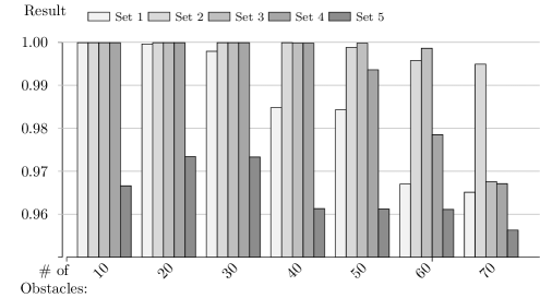
Figure 10: Results for SC3 for different sets of random obstacles

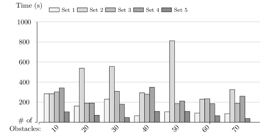
Figure 11: Solving times for SC3 for different sets of random obstacles

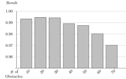
Figure 12: Accumulated results for SC3 for different sets of random obstacles

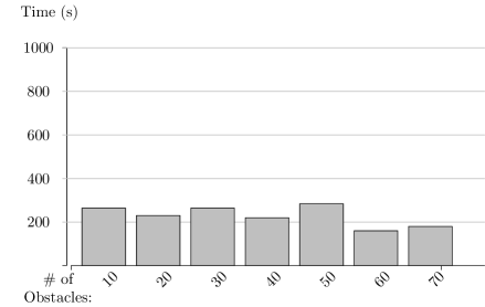
Figure 13: Accumulated solve times for SC3 for different sets of random obstacles

TABLE III: Results for SC4

	PG		Run times			MDP
#C	States	Choices	Result	Create	Model	Solve	Result
none	76676	145762	0.3997	0.22	9.2	33.1	0.9999
2	149056	292931	0.8820	0.24	23.0	64.1	0.9999

V-C Evaluation

Consider SC1: PRISM-pomdp delivers results within reasonable time only for very small examples (cf. Table I); already for the $6\times 6$ grid it runs out of memory. On the other hand, our abstraction handles grids up to $30\times 30$ within minutes, while still providing strategies with a solid accuracy. The safety probability is lower for small grids, as there is less room for R to avoid VC, and there are proportionally more situations in which R is trapped in a corner or against a wall.

For grids of any size, the safety probability computed on our abstraction is considerably higher than the naïve approach of ignoring the VC and hoping for the best: Ignoring the VC during strategy computation yields a probability of just $0.2429$ in the $3\times 3$ and $0.8209$ in the $10\times 10$ grid, compared to $0.8323$ and $0.9999$, respectively.

For the MDP, the state space for an $n\times n$ grid is in $\mathcal{O}(n^{4})$ compared to a state space in $\mathcal{O}(r^{2}n^{2})$ for the PG, where $r$ is the viewing range. As a consequence, no upper bound could be computed for the $50\times 50$ grid, as constructing the state space yielded a mem-out.

We also compare our results to SolvePOMDP, which confirms the results of PRISM-pomdp for the $3\times 3$ grid, taking 68 seconds and 107 iterations, but timed out for the $4\times 4$ grid after just 9 iterations.

In Table II, for the SC5 benchmarks, we see that the safety probability goes down for grids with a longer corridor. The reason for this effect is that, in the abstraction, R can meet VC multiple times when traveling down the corridor. To avoid this unrealistic behavior, we applied a simple history refinement as described in Sect. III-D: we divided the workspace into four evenly sized regions and have R know which region VC was visible in during the last turn. Thus, R “remembers” if VC was last seen in front or behind itself. Since the corridor is narrow enough to always observe its entire width, VC, once overtaken, can never appear in front of R again, making the safety probabilities constant independent of the length of the corridor. The same effect can be achieved by mapping the strategies obtained in the abstraction back to the original POMDP: In the resulting MC, the unrealistic behavior is no longer an issue, and safety probabilities actually increase with the length of the corridor, from $0.9962$ in the $4\times 40$ to $0.9976$ in the $4\times 100$ corridor.

Table II, SC2, indicates that the precomputation of the visibility-lookup (see Sect. IV) for large grids with many obstacles eventually takes significant time, yet the model construction time increases at a faster pace. In comparison with SC1, we see that adding obstacles decreases the number of reachable states and thus also reduces the number of choices and transitions. Eventually, model construction takes longer than the actual model checking.

Figures 10 and 11 show that obstacles – depending on their number and position – can have varied effects on the results and run times of model checking, although the accumulated results in Figure 13 show that, in general, model checking times go down as the number of obstacles increases (and therefore, the total number of reachable states decreases). Safety, on the other hand and as seen in Figure 12, is negatively affected as adding more obstacles induces additional blind spots in which R can no longer observe VC’s movement. Yet, as witnessed by Set 5, it may also provide safe areas.

Similar blind spots occur in the two rooms example, with results depicted in Table III (SC4). We add cameras to aid R by providing improved visibility around the blind spot, resulting in a near-perfect safety probability. The improved visibility doubles the state space size and increases the model checking time by about 40 seconds.

Finally, we use the two rooms example to visualize the strategy computed by our approach in Fig. 14. In each subfigure, one can see the steps taken by R so far, as well as the position of VC in the current step as simulated by the abstraction. One would expect R to try and move away from VC as far as possible, as seen in Fig. 14b, but Figs. 14a, 14c and 14d actually show the opposite: VC appears on the edge of R’s view range and R moves towards it, as, due to the abstraction, VC’s behavior gets actually more powerful when it cannot be observed. In the abstraction, it is beneficial for R to keep VC within the view range, where the VC behavior is merely probabilistic and not non-deterministic.

(a)

(b)

(c)

(d)

(e)

Figure 14: Possible movements of R and VC under the strategy computed (for SC4).

VI Discussion

Game-based abstraction successfully prunes the state space of MDPs by merging similar states. By adding an adversary that assumes the worst-case state, a PG is obtained. In general, abstraction turns the POMDP at hand into a partially observable PG, which remains intractable. However, splitting according to observational equivalence leads to a fully observable PG. PGs can be analyzed by black-box algorithms as implemented, e. g., in PRISM-games, which also returns an optimal strategy. The strategy from the PG can be applied to the POMDP, which yields the actual (higher) safety level.

In general, the abstraction can be too coarse; however, in the examples above, we have successfully shown that the game-based abstraction is not too coarse if one makes some assumptions about the POMDP. These assumptions are often naturally fulfilled by motion planning scenarios.

The assumptions from Sect. III-A can be relaxed in several respects: Our method naturally extends to multiple moving obstacles. We restricted the method to a single controllable agent, but if information is shared among multiple agents, the method is applicable also to this setting. If information sharing is restricted, special care has to be taken to prevent information leakage. Richer classes of behavior for the obstacles, including non-deterministic choices, are an important area for future research. Non-deterministic moving obstacles, for instance, lead to partially observable PGs, and game-based abstraction yields three-player games. As two sources of non-determinism are uncontrollable, both the obstacles and the abstraction can be controlled by Player 2, thus yielding a PG again.

Supporting a richer class of specifications is another option: PRISM-games supports a probabilistic variant of alternating (linear-) time logic extended by rewards and trade-off analysis. With the same abstraction technique presented here, a larger class of properties can be analyzed. However, care has to be taken when combining invariants and reachability criteria arbitrarily, as they involve under- and over-approximations.

Our method can be generalized to POMDPs for other settings. We use the original problem statement on the graph only to motivate the correctness. The abstraction can be lifted (as indicated by Def. 8), for refinement, however, a more refined argument for correctness is necessary.

The proposed PG construction is straightforward and currently realized without constructing the POMDP first. This approach simplifies the implementation of the refinement, as for large grids the POMDP can be considerably larger than the abstraction. If the POMDP is small enough to handle, we can build it, too, and map the strategy from the abstraction to the original model to obtain the precise safety probability (cf. the $(p+\tau)$-safety in Fig. 1).

VII Conclusion

We developed a game-based abstraction technique to synthesize strategies for a class of POMDPs. This class encompasses typical grid-based motion planning problems under restricted observability of the environment. For these scenarios, we efficiently compute strategies that allow the agent to maneuver the grid in order to reach a given goal state while at the same time avoiding collisions with faster moving obstacles. Experiments show that our approach can handle state spaces up to three orders of magnitude larger than general-purpose state-of-the-art POMDP solvers in less time, while at the same time using less states to represent the same grid sizes.

References

- [1] L. P. Kaelbling, M. L. Littman, and A. R. Cassandra, “Planning and acting in partially observable stochastic domains,” Artificial Intelligence, vol. 101, no. 1, pp. 99–134, 1998.
- [2] S. Thrun, W. Burgard, and D. Fox, Probabilistic Robotics. The MIT Press, 2005.
- [3] T. Wongpiromsarn and E. Frazzoli, “Control of probabilistic systems under dynamic, partially known environments with temporal logic specifications,” in CDC. IEEE, 2012, pp. 7644–7651.
- [4] G. Shani, J. Pineau, and R. Kaplow, “A survey of point-based POMDP solvers,” Autonomous Agents and Multi-Agent Systems, vol. 27, no. 1, pp. 1–51, 2013.
- [5] M. Kwiatkowska, G. Norman, and D. Parker, “Prism 4.0: Verification of probabilistic real-time systems,” in CAV, ser. LNCS, vol. 6806. Springer, 2011, pp. 585–591.
- [6] C. Dehnert, S. Junges, J. Katoen, and M. Volk, “A storm is coming: A modern probabilistic model checker,” in CAV, ser. LNCS, vol. 10427. Springer, 2017, pp. 592–600.
- [7] O. Madani, S. Hanks, and A. Condon, “On the undecidability of probabilistic planning and related stochastic optimization problems,” Artificial Intelligence, vol. 147, no. 1-2, pp. 5–34, 2003.
- [8] G. Norman, D. Parker, and X. Zou, “Verification and control of partially observable probabilistic systems,” Real-Time Systems, vol. 53, no. 3, pp. 354–402, 2017.
- [9] K. Azizzadenesheli, A. Lazaric, and A. Anandkumar, “Reinforcement learning of POMDPs using spectral methods,” CoRR, vol. abs/1602.07764, 2016. [Online]. Available: http://arxiv.org/abs/1602.07764
- [10] R. A. Howard, Dynamic Programming and Markov Processes, 1st ed. The MIT Press, 1960.
- [11] T. Chen, V. Forejt, M. Z. Kwiatkowska, D. Parker, and A. Simaitis, “PRISM-games: A model checker for stochastic multi-player games,” in TACAS, ser. LNCS, vol. 7795. Springer, 2013, pp. 185–191.
- [12] M. Kattenbelt and M. Huth, “Verification and refutation of probabilistic specifications via games,” in FSTTCS, ser. LIPIcs, vol. 4. Schloss Dagstuhl, 2009, pp. 251–262.
- [13] M. Kattenbelt, M. Kwiatkowska, G. Norman, and D. Parker, “A game-based abstraction-refinement framework for Markov decision processes,” Formal Methods in System Design, vol. 36, no. 3, pp. 246–280, 2010.
- [14] B. Braitling, L. M. F. Fioriti, H. Hatefi, R. Wimmer, H. Hermanns, and B. Becker, “Abstraction-based computation of reward measures for Markov automata,” in VMCAI, ser. LNCS, vol. 8931. Springer, 2015, pp. 172–189.
- [15] K. Chatterjee, M. Chmelík, R. Gupta, and A. Kanodia, “Qualitative analysis of POMDPs with temporal logic specifications for robotics applications,” in ICRA. IEEE, 2015, pp. 325–330.
- [16] K. Chatterjee, M. Chmelík, and M. Tracol, “What is decidable about partially observable Markov decision processes with -regular objectives,” Journal of Computer and System Sciences, vol. 82, no. 5, pp. 878–911, 2016.
- [17] K. Chatterjee, M. Chmelík, R. Gupta, and A. Kanodia, “Optimal cost almost-sure reachability in POMDPs,” Artificial Intelligence, vol. 234, pp. 26–48, 2016.
- [18] H. Yu and D. P. Bertsekas, “Discretized approximations for POMDP with average cost,” in UAI. AUAI Press, 2004, p. 519.
- [19] S. Giro and M. N. Rabe, “Verification of partial-information probabilistic systems using counterexample-guided refinements,” in ATVA, ser. LNCS, vol. 7561. Springer, 2012, pp. 333–348.
- [20] X. Zhang, B. Wu, and H. Lin, “Assume-guarantee reasoning framework for MDP-POMDP,” in CDC. IEEE, 2016, pp. 795–800.
- [21] ——, “Counterexample-guided abstraction refinement for POMDPs,” CoRR, vol. abs/1701.06209, 2017.
- [22] S. Carr, N. Jansen, R. Wimmer, J. Fu, and U. Topcu, “Human-in-the-loop synthesis for partially observable Markov decision processes,” in ACC. IEEE, 2018, pp. 762–769.
- [23] C. Amato, D. S. Bernstein, and S. Zilberstein, “Optimizing fixed-size stochastic controllers for POMDPs and decentralized POMDPs,” Autonomous Agents and Multi-Agent Systems, vol. 21, no. 3, pp. 293–320, 2010.
- [24] S. Junges, N. Jansen, R. Wimmer, T. Quatmann, L. Winterer, J. Katoen, and B. Becker, “Finite-state controllers of POMDPs via parameter synthesis,” in UAI. AUAI Press, 2018.
- [25] M. Svorenová and M. Kwiatkowska, “Quantitative verification and strategy synthesis for stochastic games,” Eur. J. Control, vol. 30, pp. 15–30, 2016.
- [26] S. Patil, G. Kahn, M. Laskey, J. Schulman, K. Goldberg, and P. Abbeel, “Scaling up Gaussian belief space planning through covariance-free trajectory optimization and automatic differentiation,” in Algorithmic Foundations of Robotics XI. Springer, 2015, pp. 515–533.
- [27] B. Burns and O. Brock, “Sampling-based motion planning with sensing uncertainty,” in ICRA. IEEE, 2007, pp. 3313–3318.
- [28] A. Bry and N. Roy, “Rapidly-exploring random belief trees for motion planning under uncertainty,” in ICRA. IEEE, 2011, pp. 723–730.
- [29] C.-I. Vasile, K. Leahy, E. Cristofalo, A. Jones, M. Schwager, and C. Belta, “Control in belief space with temporal logic specifications,” in CDC. IEEE, 2016, pp. 7419–7424.
- [30] K. Hauser, “Randomized belief-space replanning in partially-observable continuous spaces,” in Algorithmic Foundations of Robotics IX. Springer, 2010, pp. 193–209.
- [31] M. P. Vitus and C. J. Tomlin, “Closed-loop belief space planning for linear, Gaussian systems,” in ICRA. IEEE, 2011, pp. 2152–2159.
- [32] D. K. Grady, M. Moll, and L. E. Kavraki, “Extending the applicability of POMDP solutions to robotic tasks,” IEEE Trans. on Robotics, vol. 31, no. 4, pp. 948–961, 2015.
- [33] L. Winterer, S. Junges, R. Wimmer, N. Jansen, U. Topcu, J. Katoen, and B. Becker, “Motion planning under partial observability using game-based abstraction,” in CDC. IEEE, 2017, pp. 2201–2208.
- [34] C. Baier and J.-P. Katoen, Principles of Model Checking. MIT Press, 2008.
- [35] A. Condon, “The complexity of stochastic games,” Information and Computation, vol. 96, no. 2, pp. 203–224, 1992.
- [36] S. M. Ross, Introduction to Stochastic Dynamic Programming. Academic Press, Inc., 1983.
- [37] L. de Alfaro and P. Roy, “Magnifying-lens abstraction for Markov decision processes,” in CAV, ser. LNCS, vol. 4590. Springer, 2007, pp. 325–338.
- [38] E. Walraven and M. T. J. Spaan, “Accelerated vector pruning for optimal POMDP solvers,” in AAAI. AAAI Press, 2017, pp. 3672–3678.