OCU-PHYS-469, AP-GR-141
Non-linear collisional Penrose process
– How large energy can a black hole release? –
Abstract
Energy extraction from a rotating or charged black hole is one of fascinating issues in general relativity. The collisional Penrose process is one of such extraction mechanisms and has been reconsidered intensively since Bañados, Silk and West pointed out the physical importance of very high energy collisions around a maximally rotating black hole. In order to get results analytically, the test particle approximation has been adopted so far. Successive works based on this approximation scheme have not yet revealed the upper bound on the efficiency of the energy extraction because of lack of the back reaction. In the Reissner-Nordström spacetime, by fully taking into account the self-gravity of the shells, we find that there is an upper bound on the extracted energy, which is consistent with the area law of a black hole. We also show one particular scenario in which the almost maximum energy extraction is achieved even without the Bañados-Silk-West collision.
E01, E31
1 Introduction
Energy extraction from a black hole is one of the interesting and important issues not only in general relativity but also in astrophysics (engines of -ray bursts, energy sources of jets from AGN, origins of ultra-high-energy cosmic rays, etc.). In 1969 Penrose1969 , Penrose pointed out that it is possible to extract the rotational energy of a Kerr black hole, which is a stationary and axi-symmetric rotating black hole, through the decay of a particle falling from the infinity to create two particles in the ergo-region, in the case that one is bounded with negative energy, whereas the other escapes to infinity with positive energy. Successive works revealed that this mechanism does not work quite efficiently in the astrophysical situation Bardeen1972 ; Wald1974 . A bit modified version of the Penrose process called the collisional Penrose process, in which two particles collide with each other in the ergo-region instead of a single particle decay, was first noticed by Piran, Shaham and Katz Piran1975 , but its efficiency as modest as the original process was reported.
Recently, the collisional Penrose process again attracts people since Bañados, Silk and West (BSW) showed that there is no upper bound on the center-of-mass energy of two particles colliding with each other almost at the event horizon of an extremal Kerr black hole Banados2009 . This fact does not necessarily mean the unbounded energy extraction from the black hole, as the particle escaping to the infinity wastes its energy to run up the deep gravitational potential. Nevertheless, some works consistently show that fine-tuned parameters of the particles result in the energy output about 14 times larger than the input energy Bejger2012 ; Harada2012 ; Schnittman2014 ; Ogasawara2015 ; Leiderschneider2016 ; Zaslavskii2016 . It is worthwhile to notice that the same conclusion is derived even though the deformation of the event horizon caused by energetic particles swallowed by the black hole is taken into account in accordance with the hoop conjecture Hod2016 . More efficient extraction mechanism of the energy from a black hole, which has been named the super-Penrose process, was suggested Berti2014 ; Patil2015 , but there is still an argument Leiderschneider2016 .
In order to know how large energy a black hole can really release through the Penrose process, one should fully take into account the nonlinearity of the Einstein equations. It is much complicated and not so easy to treat a Kerr black hole with the gravitational backreaction by the particles. Here it is worthwhile to notice that the similar phenomenon to the BSW collision Zaslavskii2010 and the collisional Penrose process Zaslavskii2012 ; Nemoto2013 can occur in the case of the Reissner-Nordström black hole which is a spherically symmetric charged black hole. The BSW collision can also occur between two infinitesimally thin charged dust shell concentric to the Reissnr–Nordström black hole although non-linear effects are taken into account through Israel’s formalism Kimura2011 . In this paper, we shall study the collisional Penrose process in the similar situation to that studied in Ref. Kimura2011 and analyze the energy extraction efficiency.
This paper is organized as follows. In Section 2, we explain our setup and derive the equations of motion for a spherically symmetric infinitesimally thin charged shell in accordance with Israel’s formalism. Also in this section, we derive the formulation to get the conditions of two thin shells concentric with each other just after a collision with the mass transfer by imposing the 4-momentum conservation. We estimate the maximum extraction from the central black hole by analytic means in Section 3. Section 4 is devoted to concluding our analyses.
We adopt the abstract index notation: small Latin indices indicate a type of a tensor, whereas Greek indices denote components of a tensor with respect to the coordinate basis vector Wald . We also adopt the signature of the metric and the convention of the Riemann tensor used in Ref. Wald . The geometrized unit is adopted.
2 Setup and basic equations
2.1 Setup
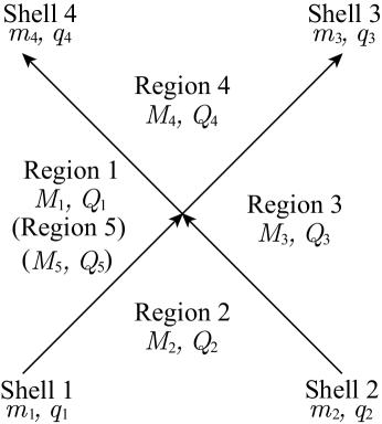
We consider two spherically symmetric shells concentric with each other. Each shell is infinitesimally thin and generates a timelike hypersurface through its motion. We will often refer this hypersurface as a shell. These shells will collide with each other, and divide the spacetime into four regions (see Fig.1). Before the collision, we call these shells Shell 1 and Shell 2, respectively. After the collision, the shell which faces on a region together with Shell 2 is called Shell 3, and the other shell is called Shell 4. The region whose boundary is formed by Shell 1 and Shell 4 is called Region 1, while the region between Shell 1 and Shell 2 is called Region 2. Similarly, the region whose boundary is formed by Shell 2 and Shell 3 is called Region 3, and the region between Shell 3 and Shell 4 is called Region 4. For notational convenience, Region 1 is often called Region 5. Hereafter, we use capital Latin indices, , and , to specify a shell or a region: runs from to , takes the values and , which represents the shells before the collision, and and , labeling the shells after the collision.
2.2 Equations of motion for shells
Let be a unit outward space-like vector normal to Shell , and define the projection operator as . Each shell is characterized by the surface stress-energy tensor which is given by
where is a Gaussian normal coordinate ( on the shell).
The extrinsic curvature of a timelike hypersurface generated by the motion of Shell is defined by
where is the covariant derivative.
The Einstein equations lead to the jump condition for the extrinsic curvatures and the conservation law for Israel :
| (1) | ||||
| (2) |
and
| (3) |
where the quantity with the subscript is defined in the region to which the unit normal points, whereas that with the subscript is evaluated on another side.
Now let us turn the spherically symmetric case. We assume that the line element in Region is given in the form
| (4) |
where is not specified in this section so that the results obtained here is applicable to various cases: a vacuum spacetime, one with the Maxwell field, one with a cosmological constant, and so on.
The components of the 4-velocity of Shell are expressed as
| (5) |
where an over dot represents a derivative with respect to the proper time naturally defined on the shell. Here note that the time coordinate, , is not continuous across the shell, although the circumferential radius, , the azimuthal angle, , and the polar angle, , are everywhere continuous. Hence two different time coordinates are assigned to each shell, and there are two kinds of time components of the 4-velocity. Using these components of the 4-velocity, we obtain the components of the unit vector normal to Shell as
| (6) |
The surface-stress-energy tensor of the spherical shell takes the following form
where is the surface energy density, corresponds to the tangential pressure, and is the 2-sphere metric with the radius . Then the conservation law (3) leads to
| (7) |
where
| (8) |
is the proper mass of Shell . In the case of , we often call Shell a dust shell and Eq. (7) implies that is constant. On the other hand, in the case of non-vanishing , depends on the proper time, if the shell is moving. We assume the reasonable energy conditions, so that .
Now, we assume the outward normal which is directed from region to region , whereas the direction of is from region to region . This assumption implies, together with Eq. (6), that the circumferential radius is increasing across the shell (shell ) from region (region ) to region (region ). Then, the junction condition (1) leads to
| (9) |
and
| (10) |
where
| (11) | ||||
| (12) |
As shown later, corresponds to the specific Misner-Sharp (MS) energy Misner1964 (MS energies per unit mass) of Shell .
2.3 Momentum conservation
In order to determine the motions of the shells after the collision, we impose the “momentum conservation” at the collision event;
| (17) |
where is the conserved total 4-momentum of two shells (see Appendix A). Using this conservation law (17), in what follows, we will show how and are determined when and are fixed. The 4-velocities and contain the information carried by two shells after collision, as we will show the details later.
For this purpose, we write down in the linear combination form of and , and describe the components of with respect to the coordinate basis in Region 3. This is because the components of and with respect to the coordinate basis in Region 3 are given as the initial data before the collision. We also write down in the linear combination form of and and describe the components of with respect to the coordinate basis in Region 1 by the similar reason.
In general, scattering problems are extremely simplified in the center of mass frame. Hence, we define the dyad basis corresponding to the center of mass frame as
| (18) | ||||
| (19) |
where
Here, we write the 4-velocities of Shell 3 and Shell 4 in the form
| (20) | ||||
| (21) |
The dyad components of the momentum conservation (17) lead to
| (22) | ||||
| (23) |
From Eqs. (22) and (23), we have
| (24) | ||||
| (25) |
By subtracting each side of Eq. (25) from that of Eq. (24), we have
and hence
| (26) |
By the similar manipulation, we also have
| (27) |
Since we consider the situation of Fig. 1, is positive, whereas is negative;
| (28) |
If we assume the proper masses and of the shells after the collision, and are determined by Eqs. (20) and (21) with the coefficients given by Eqs. (26)–(28). By using Eqs. (18) and (19), we write down in the form of the linear combination of and .
In order to write down the components of , we first replace and in and by the linear combinations of and . For notational simplicity, we introduce
| (29) | ||||
| (30) |
We have
| (31) | ||||
| (32) |
From the normalizations of and and the above equations, we have
| (33) |
Since and are desicribed by the linear combinations of and by using Eqs. (31) and (32), can also be described by the linear combinations of and through Eq. (20). We also perform the similar manipulation for by using
| (34) | ||||
| (35) |
As a result, we have
| (36) | ||||
| (37) |
where
| (38) | ||||
| (39) | ||||
| (40) | ||||
| (41) |
2.4 Components with respect to the coordinate basis
From Eqs. (36) and (37), we obtain the components of with respect to the coordinate basis in Region 3 and those of with respect to the coordinate basis in Region 1, writing down the components of and with respect to the coordinate basis in Region 3 as
| (42) | ||||
| (43) |
and the components of and with respect to the coordinate basis in Region 1 as
| (44) | ||||
| (45) |
where for notational simplicity, we introduce
| (46) | ||||
| (47) |
When we write and as
| (48) |
and
| (49) |
where
| (50) | ||||
| (51) |
we find the relation between and . Note that , which correspond to the specific Killing energies for test particles, may describe the energies of the shells but they are not conserved because of self-gravity effects of the shells.
Hereafter, all components are evaluated at , i.e., at the collision event. By using Eqs. (43)–(48), Eq. (36) leads to
| (52) | ||||
| (53) |
By using Eqs. (43)–(48), Eq. (37) leads to
| (54) | ||||
| (55) |
The components of , , and with respect to the coordinate basis in Region 2 are given by
| (56) | ||||
| (57) | ||||
| (58) | ||||
Using these components, Eqs. (29) and (30) lead to
| (59) | ||||
| (60) |
Once we know the initial conditions of shells just before the collision ( and at the collision event) and the masses of shells just after the collision, , we can obtain and by Eqs. (26)–(28), and by Eqs. (59) and (60), and then by Eqs. (52)–(41); Note that the information about is equivalent to and , whereas that about is equivalent to and . By the definition of , the value of the metric function at the collision event is given by
| (61) |
We will use Eq. (61) for deriving the mass parameter of Region 4 in the next section.
3 Maximum energy extraction by the collision of charged shells
Here we consider the situation in which the collision of two spherical shells occurs around a Reissner-Nordström black hole. Each shell is assumed to be concentric to the black hole which is located in Region 1. Then, we study the maximum energy extraction from the black hole through the collisional Penrose process by two shells: Shell 4 falls into the black hole, whereas Shell 3 goes away to the infinity with the energy larger than the total energy carried initially by Shell 1 and Shell 2. In the test-shell limit , the present system recovers the situations studied in Refs. Zaslavskii2012 ; Nemoto2013 .
The metric function of Region is given by
where and are the mass and charge parameters, respectively. The gauge one-form in the region is given by
The charge of Shell is denoted by . Gauss’s law leads to
or equivalently
The above equations lead to the conservation of total charge through the collision:
| (62) |
Equation (61) leads to
In the case of the spherically symmetric system, almost all of the quasi-local energies proposed until now agree with the so-called Misner-Sharp energy Misner1964 . In the present case, the Misner-Sharp energy within the sphere with the circumferential radius is given by
| (63) |
Hence, the Misner-Sharp energy carried by Shell is given by
If Shell has a non-vanishing charge, depends on the radius due to the electric interaction. Then the energies of Shell 1, Shell 2 and Shell 3 found by the observers at infinity, are given by
| (64) | ||||
| (65) | ||||
| (66) |
where
Before proceeding to the non-linear analysis, it is intriguing to consider the case in which the test-shell approximation is applicable. In this case, is regarded as the charge parameter of the fixed background spacetime, whereas is the charge of Shell 3 going away to the infinity. Here, we assume , and it should be noted that as long as the charge conservation (62) holds, Shell 3 can have arbitrary large charge fixing under the test-shell approximation. Thus, if very large amount of charge is transferred from Shell 4 to Shell 3 by the collision so that and then the extracted energy can be much larger than the initial total energy of the shells , the large amount of energy is extracted from the black-hole spacetime [see Eq. (66)]. There is no upper bound on the efficiency of the energy extraction, which is defined by
| (67) |
This is the case pointed out by Zaslavskii Zaslavskii2012 . If we take into account the non-linearity of the shell contribution, it is not trivial whether there exist an upper bound on the efficiency or not, although the extracted energy is finite since holds.
3.1 Upper bound on the extracted energy
Now we evaluate the upper bound on by using the fact that the Misner-Sharp energy has a non-decreasing nature with respect to , i.e., in the direction of just on Shell Hayward1994 . From Eq. (63), the following inequality should hold;
| (68) |
From Eq. (68), we have
If the central black hole is extremal, i.e., , and vanishes, we have
Then the collision at the horizon radius in Region 1 gives the largest upper bound:
| (69) |
This is also easily understood from the view of the irreducible mass of the initial black hole. Since the initial black hole is described by an extremal Reissner-Nordström solution with the mass , the irreducible mass is given by . The rest energy is one from electromagnetic contribution and can be extracted by some mechanism. As a result, The extracted energy is bounded by , which is Eq. (69).
Inequality (69) leads to
| (70) |
Since Shell 4 will be absorbed into the black hole, the black hole eventually becomes charge-neutral. Then, the area of its event horizon is larger than which is equal to the initial value of the extremal BH. This result is consistent to the area law of the event horizon.
It should be noted that the largest upper bound on is achieved by the collision on the event horizon. This fact seems to imply that the BSW type collision is a necessary condition for the large efficiency in contrast to the test particle case. However, we will see in the following example that it is not necessarily the case.
3.2 An example of almost maximum energy extraction
In this subsection, we focus on the case of and . By this restriction, the expressions of the energy-momentum transfer through the collision become so simple that we obtain analytically an example of almost maximum energy extraction. The same system has been studied by Ida and one of the present authors Ida1999 , although they has not focused on the collisional Penrose process.
We have
| (71) | ||||
| (72) | ||||
| (73) | ||||
| (74) |
Substituting Eqs. (71)–(74) into Eqs. (52)–(55) and by using Eqs. (103)–(106), we have
| (75) | ||||
| (76) | ||||
| (77) | ||||
| (78) |
It is worthwhile to notice that and hold because of . Note also that holds by its definition, and hence and hold.
We again assume that the black hole is initially extremal and finally charge-neutral as a result of the absorption of Shell 4 by the black hole:
| (79) |
Furthermore, we assume
| (80) |
Since we assume the collision takes place near the horizon, we write the circumferential radius at the collision event, , in the form of
| (81) |
with .
Hereafter, a character with a tilde denotes a quantity normalized by the initial mass of the black hole, , i.e., and . Since Shell 1 and Shell 2 approach the black hole from infinity, should be larger than or equal to unity. We focus on the case that is of order unity.
Together with Eqs. (79)–(81), Eq. (75) leads to
| (82) |
The assumptions (79)–(81) lead to
| (83) | ||||
| (84) |
Since the collision should occur outside the black hole, we have from Eqs. (83) and (84) the following constraints
| (85) | ||||
| (86) |
Equation (85) implies that should be at most of order , and then Eq. (86) implies that both of and should also be at most of order . Hereafter we assume
We consider the situation in which holds at the collision event. Then, is approximately estimated at
| (87) | ||||
| (88) |
Therefore, the asymptotic energy of Shell 3 is given by
| (89) |
which gives the energy extracted from the system explicitly as
| (90) |
As we discussed in §3.1, the upperbound is given by Eq. (69). If the asymptotic specific energies and are not so large, i.e., , the above energy extraction (90) gives almost maximal value if (the collision occurs near the horizon). The present result implies that the collisional Penrose process of two charged shells with very small masses can achieve the almost maximum energy extraction, if the black hole becomes finally charge-neutral.
As for the efficiency of the energy extraction , we have :
| (91) |
Equation (91) implies that there is no upper bound on . This is because the maximally extracted energy is finite even if the input initial energy of two shells, , is infinitely small.
We also have
| (92) |
which guarantees the consistency with the area law of the black hole because , as mentioned below Eq. (70).
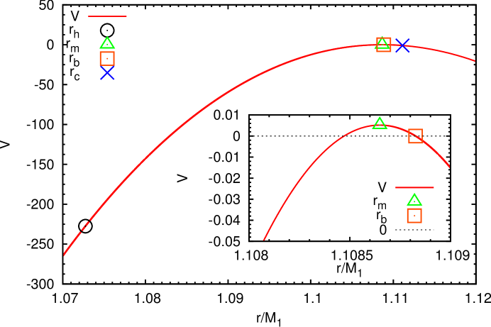
In order to extract the energy from a black hole, in addition to the above energy argument, we must impose one additional condition, which is that Shell 3 must move outward to infinity. However, by the reason mentioned below Eq. (78), implies just after the collision. Hence Shell 3 has to bounce off the potential barrier so that it goes away to infinity. As shown below, this bounce will happen under some possible condition.
From Eq. (10), the energy equation of Shell 3 is written in the form,
where the effective potential is given by
| (93) |
with introducing a function defined by
The function has a zero point and a maximum at the identical circumferential radius in the domain of . By using Eq. (90), we find
| (94) |
or the explicit form up to the second order of as
| (95) |
The metric function is rewritten in the form
It is easy to see that is a monotonically increasing function in the domain . The larger root of corresponds to the horizon radius in Region 3;
| (96) | ||||
| (97) |
From Eq. (86), we have
which leads to, together with Eqs. (95) and (97),
| (98) | ||||
| (99) |
as shown the details in Appendix B.
In order for Shell 3 to bounce off before the horizon, we impose a sufficient condition, which is , which gives one additional condition for and such that
| (100) |
With this condition, we find
| (101) |
and
Since and hold, we have . It is not so difficult to obtain . Together with the inequality (101), these facts imply that Shell 3 initially moving to the black hole should bounce off at the potential barrier with the circumferential radius which satisfies , and then go away to the infinity. Shell 3 can carry the huge energy extracted from the black hole to the infinity.
We should recognize that the condition (100) gives a constraint on the initial energies of two shells (and charge of Shell 2). If we wish to get the large efficiency, the initial energies must be small. This is because the maximum extracted energy is finite and fixed, and the efficiency becomes large if the initial energies are small. Note that the inequality (100) is consistent with Eqs. (85) and (86).
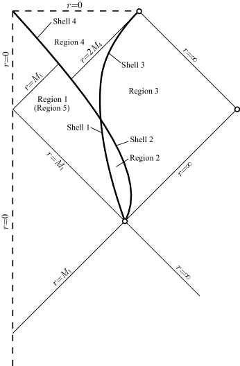
In Fig. 2, we depict the Penrose diagram of the spacetime in which the collision described in this subsection occurs. Two massive charged shells are initially falling toward an extremal Reissner-Nordström black hole, and then collide near the horizon. After a large amount of charge transfer at the collision, Shell 3 will bounce off at the potential barrier and then goes away to infinity with a huge amount of energy. The finial spacetime turns to be a neutral Schwarzschild black hole.
Here, we should note that the BSW collision does not occur in the present situation, where the BSW collision means that the center-of-mass energy at the collision near the horizon becomes unboundedly large, i.e., diverges in the limit of . As we show in Appendix C, does not diverge as in the present example, although we find the almost maximum energy extraction from the black hole.
4 Conclusion
We have investigated the energy extraction process from a Reissner-Nordström black hole through the collision of two spherical charged shells by taking into account the self-gravity of the shells. We have derived the conditions for the shells just after the collision by imposing the conservation of total 4-momentum, where the mass and charge transfers between the shells are allowed. Then, from the monotonicity of the Misner-Sharp mass, we show that the extracted energy is bounded from above, and the upper bound is the half of the ADM energy of the initial black hole, which is consistent with the area law of the black hole. Furthermore, from this consideration, we find the following conditions for the large energy extraction;
-
1.
The collision event must be very close to the event horizon;
-
2.
The initial black hole is nearly the extremal Reissner-Nordström one;
-
3.
The final spacetime is a charge-neutral Schwarzschild black hole.
Finally, we have shown one scenario of almost maximum energy extraction, in which the BSW collision does not take place.
As for the BSW collision, as we have shown one example in Appendix C, we expect that it will not lead to the maximum energy extraction. The collision with the infinite center-of-mass energy may take place inside the horizon radius which is necessarily larger than the initial horizon radius . In order to extract the energy, the collision point must be outside the horizon. Here we should again note that the collision event at will be a necessary condition for the maximum energy extraction. Hence the BSW collision will not achieve it. However, if a BSW-like collision is possible, which means the center-of-mass energy is not infinite but very large, so that large energy extraction is possible, we may find new particle with large mass through a collision near a black hole horizon similar to the process found by Nemoto et al by invoking the test particle approximation Nemoto2013 , and reveal new aspect of high energy physics. The work on a BSW-like collision in the present model with two charged shells and the possible energy extraction will be published elsewhere.
Since an extremely charged black hole may not exist in nature, it is more interesting to study a rapidly rotating black hole with collisional spinning particlesspinning1 ; spinning2 ; spinning3 ; spinning4 . If we can extract the maximum energy determined by the irreducible mass, i.e.,
by the collisional Penrose process, we will find most effective energy extraction method from a rotating black hole. This study is also in progress.
Acknowledgments
This work was supported in part by JSPS KAKENHI Grant Numbers JP25400265 (KN), JP16K05362 (KM), 17H06357 (KM) and JP17H06359 (KM).
Appendix A Consistency check of momentum conservation
It should be noted that, by the definition of and , i.e., Eqs. (11) and (12), the following relation is trivially satisfied at the collision event:
| (102) |
Since it seems to be non-trivial whether the relation (102) is consistent with the momentum conservation (17), which is our ansatz, we will show in this appendix that it is the case.
It is impossible to directly derive Eq. (102) from Eqs. (52), (53), (54) and (55) obtained from the momentum conservation (17), and hence we rewrite them in the appropriate form for our purpose. There are several useful relations derived by using Eq. (9);
| (103) | ||||
| (104) | ||||
| (105) | ||||
| (106) |
By using the above relations, Eqs. (52), (53), (54) and (55) are rewritten in the form
| (107) | ||||
| (108) | ||||
| (109) | ||||
| (110) |
Then, by using Eqs. (22), (23) and (26), Eqs. (107) and (109) lead to Eq. (102).
Appendix B Additional sufficient condition for the bounce of Shell 3
To make the analysis simple, we introduce the following three parameters,
| (111) |
satisfying and .
| (112) | ||||
| (113) |
Eq. (86) under the condition yields
| (114) |
which leads to, together with Eqs. (95) and (113),
| (115) | ||||
| (116) |
Therefore, the following relation among parameters becomes a sufficient condition for Shell 3 to bounce off:
| (117) |
which gives one additional condition (100) imposed in the text.
Appendix C BSW collision v.s. non-BSW collision
The BSW collision is defined as that with the extremely large collision energy in the center of mass frame. The collision energy in the center of mass is equal to which is written in the form
The above equation implies that the large is equivalent to the large . The normalization condition of the 4-velocities of Shell 1 and Shell 2 lead to
| (118) | ||||
Hence, from Eq. (59), we have
| (119) |
We consider the collision near the horizon in Region 2, i.e., . Thus, we write the radius at the collision event in the form
| (120) |
where we have assumed : in the limit of , the collision occurs at the horizon in Region 2. We also assume . Since Eq. (119) is rewritten as
| (121) |
near the horizon (), the BSW collision implies that either or vanishes as .
Since and near the horizon, we have to evaluate and at the collision point. From the definition, we find
In our example, we can easily show that
both and are finite as follows:
Using our ansatz, and
,
we find
which yields and are finite. As a result, is also finite, and then does not diverge near the horizon. It is not the BSW collision.
When we find the BSW collision ? One of or must vanish near the horizon. Then we consider the case that with whereas is finite. This can be realized if we assume
| (122) |
Since
| (123) |
we obtain if and only if
is satisfied, where we have .
The root of the above equation, which satisfies , is
| (124) |
From the normalization condition of the 4-velocity of Shell 1, i.e., , we find
where
with
As for , we obtain , if and only if
Hence if we assume that Region 3 spacetime is not extreme, i.e., , is finite near the horizon.
We then find
| (125) |
and will diverge near the horizon, which corresponds to the BSW collision. Hence the BSW collision between Shell 1 and Shell 2 is possible in the case that Eqs. (122) and (124) are satisfied and Region 3 spacetime is not extreme. The horizon radius of Region 3 is larger than that of Region 2:
This fact implies that the present BSW collision necessarily occurs inside a black hole. In order to extract energy, the collision point must be outside the horizon. We then expect that the BSW collision may not lead to the maximum energy extraction.
References
- (1) R. Penrose, Riv. Nuovo Cim. 1, 252 (1969), [Gen. Rel. Grav.34,1141(2002)].
- (2) J. M. Bardeen, W. H. Press and S. A. Teukolsky, Astrophys. J. 178, 347 (1972).
- (3) R. M. Wald, Astrophys. J. 191, 231 (1974).
- (4) T. Piran, J. Shaham and J. Katz, Astrophys. J. Lett. 196, L107 (1975).
- (5) M. Banados, J. Silk and S. M. West, Phys. Rev. Lett. 103, 111102 (2009), [0909.0169].
- (6) M. Bejger, T. Piran, M. Abramowicz and F. Hakanson, Phys. Rev. Lett. 109, 121101 (2012), [1205.4350].
- (7) T. Harada, H. Nemoto and U. Miyamoto, Phys. Rev. D 86, 024027 (2012), [1205.7088], [Erratum: Phys. Rev.D86,069902(2012)].
- (8) J. D. Schnittman, Phys. Rev. Lett. 113, 261102 (2014), [1410.6446].
- (9) K. Ogasawara, T. Harada and U. Miyamoto, Phys. Rev. D 93, 044054 (2016), [1511.00110].
- (10) E. Leiderschneider and T. Piran, Phys. Rev. D 93, 043015 (2016), [1510.06764].
- (11) O. B. Zaslavskii, Phys. Rev. D 94, 064048 (2016), [1607.00651].
- (12) S. Hod, Phys. Lett. B759, 593 (2016), [1609.06717].
- (13) E. Berti, R. Brito and V. Cardoso, Phys. Rev. Lett. 114, 251103 (2015), [1410.8534].
- (14) M. Patil, T. Harada, K.-i. Nakao, P. S. Joshi and M. Kimura, Phys. Rev. D 93, 104015 (2016), [1510.08205].
- (15) O. B. Zaslavskii, JETP Lett. 92, 571 (2010), [1007.4598]
- (16) O. B. Zaslavskii, Phys. Rev. D 86, 124039 (2012), [1207.5209].
- (17) H. Nemoto, U. Miyamoto, T. Harada and T. Kokubu, Phys. Rev. D 87, 127502 (2013), [1212.6701].
- (18) M. Kimura, K. Nakao and H. Tagoshi, Phys. Rev. D 83, 044013 (2011), [1010.5438]
- (19) R.M. Wald, General Relativity (The University of Chicago Press, Chicago, 1984).
- (20) W. Israel, Nuovo Cim. 44B, 1 (1966).
- (21) C.W. Misner and D.H. Sharp, Phys. Rev. 136, B571 (1964).
- (22) S. A. Hayward, Phys. Rev. D 53, 1938 (1996), [gr-qc/9408002].
- (23) D. Ida and K.-i Nakao, Prog. Theor. Phys. 101, 989 (1999).
- (24) C. Armaza, M. Banados, and B. Koch, Class. Quantum Grav. 33, 105014 (2016).
- (25) O. B. Zaslavskii, Europhys. Lett. 114, 30003 (2016)
- (26) M.-Y. Guo and S.-J. Gao, Phys. Rev. D93, 084025 (2016).
- (27) Y.-P. Zhang, B.-M. Gu, S.-W. Wei, J. Yang and Y.-X. Liu, Phys. Rev. D94, 124017 (2016).
