On the dynamics of the Pappus-Steiner map

Abstract: We extract a two-dimensional dynamical system from the theorems of Pappus and Steiner in classical projective geometry. We calculate an explicit formula for this system, and study its elementary geometric properties. Then we use Artin reciprocity to characterise all sufficiently large primes $p$ for which this system admits periodic points of orders $3$ and $4$ over the field $\mathbb{F}_{p}$; this leads to an unexpected Galois-theoretic conjecture for $n$-periodic points. We also give a short discussion of Leisenring’s theorem, and show that it leads to the same dynamical system as the Pappus-Steiner theorem. The appendix contains a computer-aided analysis of this system over the field of real numbers.

AMS subject classification (2010): 51N15, 37C25.

1. Introduction

This article is a study of a two-dimensional dynamical system arising out of the Pappus-Steiner theorem in classical projective geometry. The construction of this system was inspired by Hooper [7] and Schwartz [17], but the specifics of our approach are different. We begin with an elementary introduction to the theorems of Pappus and Steiner. The results of the paper are described in Section 2.3 (on page 2.3) after the required notation is available.

1.1. Pappus’s Theorem

Let $\mathbb{P}^{2}$ denote the projective plane over a field $k$. Consider two lines $L$ and $M$ in $\mathbb{P}^{2}$, intersecting at a point $P$. Choose distinct points $A_{1},A_{2},A_{3}$ and $B_{1},B_{2},B_{3}$ on $L$ and $M$ respectively (all away from $P$), displayed as an array $\left[\begin{array}[]{ccc}A_{1}&A_{2}&A_{3}\\ B_{1}&B_{2}&B_{3}\end{array}\right]$. Then Pappus’s theorem says that the three cross-hair intersection points

$$A_{1}B_{2}\cap A_{2}B_{1},\quad A_{2}B_{3}\cap A_{3}B_{2},\quad A_{1}B_{3}\cap A_{3}B_{1},$$

corresponding to the three minors of the array, are collinear (see Diagram 1). The line containing them (called the Pappus line of the array) will be denoted by $\left\{\begin{array}[]{ccc}A_{1}&A_{2}&A_{3}\\ B_{1}&B_{2}&B_{3}\end{array}\right\}$.

diagram 1. Pappus’s theorem

A proof of Pappus’s theorem may be found in almost any book on elementary projective geometry (for instance, see [18, Ch. 1]).

1.2. Steiner’s Theorem

If we permute the bottom row of the array, then a priori we get a different Pappus line. There are six such lines corresponding to the elements of the permutation group $\mathfrak{S}_{3}$. For an element $\sigma\in\mathfrak{S}_{3}$, let

$$\Lambda_{\sigma}=\left\{\begin{array}[]{ccc}A_{1}&A_{2}&A_{3}\\ B_{\sigma(1)}&B_{\sigma(2)}&B_{\sigma(3)}\end{array}\right\}$$

denote the corresponding Pappus line. According to our convention, the permutation $(1\,3\,2)$ takes $1$ to $3$ etc., so that $\Lambda_{(1\,3\,2)}=\left\{\begin{array}[]{ccc}A_{1}&A_{2}&A_{3}\\ B_{3}&B_{1}&B_{2}\end{array}\right\}$. Now Steiner’s theorem says that the lines $\Lambda_{e},\Lambda_{(1\,2\,3)},\Lambda_{(1\,3\,2)}$, corresponding to the even permutations are concurrent, and the lines $\Lambda_{(1\,2)},\Lambda_{(1\,3)},\Lambda_{(2\,3)}$ corresponding to the odd permutations are also concurrent. In Diagram 2, the green lines correspond to the even permutations and blue lines to the odd ones. In order to reduce visual clutter, the cross-hair lines have not been shown.

diagram 2. Steiner’s theorem

A proof of Steiner’s theorem may be found in [2, p. 216] or [7, Section 5]. In summary, starting from $A_{1},\dots,B_{3}$, the entire process can be seen as:

$$\text{Two lines with three points on each}\quad\leadsto\quad\text{Two points with three lines on each}.$$

The latter structure (seen in the dual projective plane) is the same as the former, hence we will get a dynamical system (i.e., a map from a set to itself) at an appropriate level of abstraction. We begin by recalling some standard facts about cross-ratios (see [18, Ch. 1]).

1.3. Cross-ratio and the $j$-function

Given a sequence of four points $x_{1},x_{2},x_{3},x_{4}$ on the projective line $\mathbb{P}^{1}$, define their cross-ratio to be

$$\langle x_{1},x_{2},x_{3},x_{4}\rangle=\frac{(x_{1}-x_{3})(x_{2}-x_{4})}{(x_{2}-x_{3})(x_{1}-x_{4})}.$$

If $r$ denotes this value, then permuting the $x_{i}$ changes the cross-ratio into one of the six possible functions of $r$. In fact, if $x_{4}$ is left fixed then the six permutations of $x_{1},x_{2},x_{3}$ give each of these functions exactly once. If $\sigma$ denotes any of the permutations

$$e,\quad(1\,2),\quad(1\,3),\quad(2\,3),\quad(1\,2\,3),\quad(1\,3\,2),$$

then $\langle x_{\sigma(1)},x_{\sigma(2)},x_{\sigma(3)},x_{4}\rangle$ is respectively equal to

$$r,\quad 1/r,\quad r/(r-1),\quad 1-r,\quad(r-1)/r,\quad 1/(1-r).$$ (1.1)

Now define

$$j(r)=\frac{4\,(r^{2}-r+1)^{3}}{27\,r^{2}\,(r-1)^{2}}.$$

This expression remains unchanged if we substitute any of the values in (1.1) in place of $r$. In other words, if $j(r)=\tau$, then the six roots of the polynomial equation

$$4\,(Z^{2}-Z+1)^{3}-27\,\tau\,Z^{2}\,(Z-1)^{2}=0,$$

are exactly those in (1.1). Henceforth we assume that $\text{char}(k)\neq 2,3$, since the theory of cross-ratios has more pitfalls in those characteristics.

2. The Pappus structure

2.1.

Define a Pappus structure in a projective plane to be an unordered pair of sets

$$\Pi=\left\{\left\{A_{1},A_{2},A_{3}\right\},\left\{B_{1},B_{2},B_{3}\right\}\right\},$$ (2.1)

such that

1. the six points $A_{1},\dots,B_{3}$ are pairwise distinct,

2. the three points in each set are collinear,

3. the line containing the first three is different from the line containing the other three, and

4. the point of intersection of the two lines (say $P$) is different from $A_{1},\dots,B_{3}$.

We will represent such a structure by a pair of numbers, called its signature. The process followed in Steiner’s theorem, when applied to the signature, will give a dynamical system.

2.2.

Given a Pappus structure $\Pi$, consider the cross-ratios

$$r=\langle A_{1},A_{2},A_{3},P\rangle,\qquad s=\langle B_{1},B_{2},B_{3},P\rangle,$$

and write

$$x=j(r)+j(s),\qquad y=j(r)\,j(s).$$

Definition 2.1.

The ordered pair $[x,y]$ will be called the signature of $\Pi$, denoted $\text{sig}(\Pi)$.

It is well-defined by what we have said above. The intuition behind this definition is two-fold:

• since the order of the three points within the line is irrelevant, we pass from the cross-ratio to its $j$-function, and

• since the two lines are on equal footing, we pass from $j(r)$ and $j(s)$ to their elementary symmetric functions.

Suppose that we have two Pappus structures $\Pi_{1}$ and $\Pi_{2}$, whose points come from possibly different planes $\mathbb{P}^{2}_{(1)}$ and $\mathbb{P}^{2}_{(2)}$.

Definition 2.2.

We define $\Pi_{1},\Pi_{2}$ to be equivalent, if there is an isomorphism $\mathbb{P}^{2}_{(1)}\rightarrow\mathbb{P}^{2}_{(2)}$ carrying $\Pi_{1}$ to $\Pi_{2}$.

The following result justifies the definition of the signature.

Proposition 2.3.

Two Pappus structures are equivalent, if and only if their signatures coincide.

Proof.

The ‘only if’ part is obvious, and the converse is a simple computation (see Section 7.2). ∎

Let $\Pi$ be a Pappus structure with $\text{sig}(\Pi)=[x,y]$. Assume $x\neq y$, and let

$$\text{steiner}(\Pi)=\left\{\left\{\Lambda_{e},\Lambda_{(1\,2\,3)},\Lambda_{(1\,3\,2)},\right\},\left\{\Lambda_{(1\,2)},\Lambda_{(1\,3)},\Lambda_{(2\,3)}\right\}\right\}.$$ (2.2)

We will show later (see Section 7.3) that this is a Pappus structure. Its ‘points’ come from the dual projective plane $(\mathbb{P}^{2})^{\vee}$. It is well-defined, since the starting points are permuted in all possible ways during the construction. The next theorem gives its signature.

Theorem 2.4.

With notation as above,

$$\text{sig}(\text{steiner}(\Pi))=\left[\frac{2y\,(y-x+2)}{(x-y)^{2}},\frac{y^{2}}{(x-y)^{2}}\right].$$

Proof.

See Section 7.3. ∎

Now consider the Pappus-Steiner map

$$\pi:k^{2}\;-\rightarrow k^{2},\quad[x,y]\longrightarrow\left[\frac{2y\,(y-x+2)}{(x-y)^{2}},\frac{y^{2}}{(x-y)^{2}}\right].$$ (2.3)

Of course, $\pi$ is defined only if $x\neq y$. However, one can define a subset $\mathbb{A}\subset k^{2}$ such that $\pi$ and all of its iterates are defined over it (see Section 3.1). This leads to a dynamical system $\pi:\mathbb{A}\longrightarrow\mathbb{A}$.

2.3. Results

The system $\pi$ can be studied over any ground field, and either from an analytic or an algebraic viewpoint. In this paper, we mostly do the latter.

1. The basic geometric properties of $\pi$ are given in Section 3. In particular, we show that the map interchanges two geometrically natural subsets of $\mathbb{A}$, namely the ’harmonic’ and the ’balanced’ Pappus structures. Moreover, $\pi$ has a natural involution associated to it, which carries an interesting interpretation in terms of cross-ratios.

2. One of the natural objects of study of a dynamical system is its periodic points. In Theorems 4.2 and 4.3, we characterise all (sufficiently large) primes $p$, such that $\pi$ admits periodic points of orders $3$ or $4$ over the prime field $\mathbb{F}_{p}$. The technique involves a Gröbner basis computation followed by the use of class field theory. The polynomials which emerge during the Gröbner computation seem to be unusual from a Galois-theoretic viewpoint, and this observation leads to a conjecture about the field extension generated by all $n$-periodic points.

3. The map $\pi$ has two fixed points and a $2$-cycle, and hence it is geometrically natural to consider the pencil of conics through these four points (see Section 5). We discover that there is a unique conic in this pencil which is sent by $\pi$ into another such conic. This leads to a one-dimensional quadratic dynamical system. In Section 5.4 we deduce a result about its Julia set.

4. Section 6 contains a discussion of a theorem due to Leisenring which is formally similar to Steiner’s. We show that it leads to exactly the same dynamical system as in (2.3).

5. The appendix by Attila Dénes contains a brief computer-aided analysis of the Pappus-Steiner system over real numbers.

We will use [4, 10, 18] as standard references for projective geometry. The reader is referred to [11, 13] for the necessary concepts from algebraic number theory. The basic terminology of dynamical systems may be found in [6], and that of Gröbner bases in [1].

All the algebraic computations, including those for Gröbner bases, were done in Maple and confirmed in Macaulay-2. The number-theoretic computations were done using a combination of Maple and Sage. For ease of reading, we have relegated some of the more computational proofs to Section 7.

3. The geometry of the Pappus-Steiner map

3.1.

Let $W_{1}=\{[x,y]:x=y\}$ denote the locus in $k^{2}$ over which $\pi$ is not defined. Then $\pi^{2}$ is not defined over the locus $W_{2}$ of points $[x,y]\in k^{2}\setminus W_{1}$ such that $\pi([x,y])\in W_{1}$. In general, define inductively

$$W_{n}=\{[x,y]\in k^{2}\setminus\bigcup\limits_{i=1}^{n-1}W_{i}:\pi([x,y])\in W_{n-1}\}\quad\text{for $n\geqslant 2$},$$

and write $\mathbb{A}=k^{2}\setminus\bigcup\limits_{i=1}^{\infty}W_{i}$. Then $\pi$ and all of its iterates are defined over $\mathbb{A}$, and we have a dynamical system $\pi:\mathbb{A}\longrightarrow\mathbb{A}$.

If $k$ is either the field of real or complex numbers, then $\mathbb{A}$ is a dense open subset of $k^{2}$. A calculation shows that $W_{2}$ is the union of lines $y=0,y=2x-4$, and $W_{3}$ is the curve $4x^{2}-4xy+y^{2}-8y=0$. There seems to be no easy general formula for the equation of $W_{n}$.

3.2. Balanced and Harmonic structures

We will say that a Pappus structure is balanced, if $j(r)=j(s)$; which is equivalent to $x^{2}=4y$. This is tantamount to requiring that the unordered quadruples

$$\{P,A_{1},A_{2},A_{3}\},\quad\{P,B_{1},B_{2},B_{3}\},$$

should be projectively isomorphic. Let $B=\{[x,y]\in\mathbb{A}:x^{2}=4y\}$ denote the parabola formed by balanced structures.

Recall that four points on $\mathbb{P}^{1}$ are said to be harmonic if their cross-ratio (in some order) is $-1$. We will say that $\Pi$ is harmonic, if either of the quadruples above is harmonic. This is equivalent to either $j(r)$ or $j(s)$ being $=1$, i.e., $x=y+1$. Let $H=\{[x,y]\in\mathbb{A}:x=y+1\}$ denote the line formed by harmonic structures. There is a simple but pleasing relation between these two loci:

Proposition 3.1.

With notation as above, $\pi(H)\subseteq B$ and $\pi(B)\subseteq H$.

Proof.

We have $\pi([t+1,t])=[2t,t^{2}]$, which is balanced. Similarly,

$$\pi([2t,t^{2}])=\left[\frac{2(t^{2}-2t+2)}{(t-2)^{2}},\frac{t^{2}}{(t-2)^{2}}\right],$$

which is harmonic. ∎

Hence the second iterate $\pi^{2}$ sends $H$ to $H$ and $B$ to $B$. Both maps are given by the same formula

$$\alpha(t)=\frac{t^{2}}{(t-2)^{2}}.$$ (3.1)

In Section 5.4, we will treat this as a map of one complex variable and analyse its dynamics.

3.3.

In order to investigate the image of $\pi$, we write $\pi([x,y])=[p,q]$, and try to solve for $x,y$ in terms of $p,q$. This leads to equations

$$2y(y-x+2)^{2}=p(x-y)^{2},\quad y^{2}=q(x-y)^{2}.$$

After eliminating $x$, we have

$$(p^{2}-4q)\,y^{2}-8pq\,y+16q^{2}=0,\quad x=\frac{(2q-p)y}{2q}+2.$$

If $p^{2}\neq 4q$, then we get two solutions $y=\frac{4q}{p\pm 2\sqrt{q}}$, either of which determines $x$ uniquely. If $p^{2}=4q$, then we get a unique solution

$$x=\frac{2q}{p}+1,\quad y=\frac{2q}{p}$$

in $H$. Hence we have the following proposition:

Proposition 3.2.

The map $\pi:\mathbb{A}\longrightarrow\mathbb{A}$ is a double cover ramified over $B$.

This suggests that $\mathbb{A}$ should have an involution, i.e., a function $\mathbb{A}\stackrel{{\scriptstyle\tau}}{{\longrightarrow}}\mathbb{A}$ which exchanges the two sheets of the cover. In order to find it, let $[x_{1},y_{1}],[x_{2},y_{2}]$ denote the two pre-images of $[p,q]$, so that we must have

$$x_{i}=\frac{(2q-p)y_{i}}{2q}+2\quad(i=1,2),\quad y_{1}+y_{2}=\frac{8pq}{p^{2}-4q},\quad y_{1}\,y_{2}=\frac{16q^{2}}{p^{2}-4q}.$$

After eliminating $p$ and $q$, we get

$$x_{2}=\frac{x_{1}-2y_{1}}{x_{1}-y_{1}-1},\quad y_{2}=\frac{y_{1}}{x_{1}-y_{1}-1}.$$

Hence we have the formula

$$\tau([x,y])=\left[\frac{2y-x}{y-x+1},\frac{y}{y-x+1}\right].$$

As it stands, it is only defined over $\mathbb{A}\setminus H$. However, it is natural to set $\tau([x,y])=[x,y]$ for a point in $H$.

3.4.

This involution can be interpreted at the level of Pappus structures. To see this, define

$$w^{\circ}=\frac{2-w}{1+w}$$

for $w\neq-1,2,1/2$. This operation is such that $(w^{\circ})^{\circ}=w$. The next proposition shows that it imitates the action of $\tau$ at the level of cross-ratios.

Proposition 3.3.

Let $[x,y]=[j(r)+j(s),j(r)\,j(s)]$ denote a point away from $H$. Then

$$\tau([x,y])=\left[j(r^{\circ})+j(s^{\circ}),j(r^{\circ})\,j(s^{\circ})\right].$$

Proof.

Consider the equation $Z^{2}-\frac{2y-x}{y-x+1}\,Z+\frac{y}{y-x+1}=0$. Applying the quadratic formula, one of its roots is

$$\frac{4\,(r^{2}-r+1)^{3}}{(r-2)^{2}\,(2r-1)^{2}\,(r+1)^{2}},$$

and of course, the second root is the same expression in $s$. If we write $j(z)$ for this expression, then it leads to a sextic polynomial equation in $z$ with roots

$$\frac{2-r}{r+1},\quad\frac{r+1}{2-r},\quad\frac{r+1}{2r-1},\quad\frac{2r-1}{r+1},\quad\frac{2r-1}{r-2},\quad\frac{r-2}{2r-1}.$$ (3.2)

We declare the first of these to be $r^{\circ}$, but the choice is arbitrary. One can get them all by applying the functions in (1.1) to $r^{\circ}$. ∎

The relationship between the $j$-functions of $r$ and $r^{\circ}$ is also involutive. We have

$$j(r^{\circ})=\frac{j(r)}{j(r)-1},\quad\text{and}\quad j(r)=\frac{j(r^{\circ})}{j(r^{\circ})-1}.$$

This follows by a direct computation using the formula for $r^{\circ}$.

4. Periodic points

4.1.

Let $n>0$ be an integer. Recall that a point $z=[x,y]\in\mathbb{A}$ is said to be $n$-periodic, if $\pi^{n}(z)=z$. The smallest integer $n$ for which this equation holds is called the period of $z$. A point of period $1$ is called a fixed point. If $z$ is $n$-periodic, then

$$z\rightarrow\pi(z)\rightarrow\pi^{2}(z)\rightarrow\dots\rightarrow\pi^{n}(z)=z,$$

is called an $n$-cycle.

Since $\pi$ is expressed by rational functions, it is natural to use Gröbner bases to detect the points of period $n$. Fix the polynomial ring $R=\mathbb{Q}[x,y]$ with a lexicographic term order given by $x>y$. This is suitable for eliminating the variable $y$ (see [1, Ch. 2]).

For illustration, assume $n=2$. Then the equation $\pi^{2}(z)=z$ gives the ideal

$$I_{2}=(y(4x^{2}-4xy+y^{2}-16x+7y+16),-4x^{3}+4x^{2}y-xy^{2}+20x^{2}-12xy+2y^{2}-16x-8y)$$

in $R$. A point $[x,y]$ is $2$-periodic, if and only if both polynomials in $I_{2}$ vanish on it. The Gröbner basis of this ideal is given by

$$f_{1}(x) =x(x-1)(x-2)(x-4)(x-5)(x-8)(x-12),$$

$$f_{2}(x,y) =18480y-67x^{6}+1934x^{5}-19615x^{4}+84620x^{3}-152728x^{2}+85856x.$$

Now, although this computation was carried out over $\mathbb{Q}$, this is also the Gröbner basis of $I_{2}$ (seen as an ideal in $k[x,y]$) for $\text{char}(k)$ sufficiently large. This gives the following proposition:

Proposition 4.1.

Assume that $\text{char}(k)$ is either zero or sufficiently large. Then the only fixed points of $\pi$ are $[2,1]$ and $[12,16]$. Moreover, the only points of period $2$ are $[5,4]$ and $[8,16]$, which are sent to each other by $\pi$.

Proof.

This follows by solving $f_{1}$ for $x$, and then using $f_{2}$ to find $y$. The values $x=0,1$ lead to $y=0$, which is disallowed. ∎

We are aiming for a similar theorem for the cases $n=3,4$. Assume that $k=\mathbb{F}_{p}$, for $p$ sufficiently large.

4.2. Case $n=3$

We can find the Gröbner basis of $I_{3}$ as before. It turns out to be

$$f_{1}(x)=x^{9}(x-12)(x-2)\underbrace{(x^{3}-84x^{2}+896x-1984)}_{u(x)}\underbrace{(x^{3}-48x^{2}+656x-1856)}_{v(x)},$$

(where $u(x),v(x)$ are irreducible over $\mathbb{Q}$) together with

$$f_{2}(x,y)=x^{4}\,y-\phi_{1}(x),\qquad f_{3}(x,y)=y^{2}+yx-\phi_{2}(x).$$

Here $\phi_{1}$ and $\phi_{2}$ are degree $16$ polynomials in $x$, which are too cumbersome to write down in full. Then one checks that $x=0$ is not an admissible value, and $x=2$ and $12$ lead to the fixed points which we have already found. Moreover, if we substitute the value of $y$ obtained from $f_{2}$ into $f_{3}$, then the latter vanishes identically modulo $f_{1}$. Hence there exists a point of period $3$, exactly when either $u(x)$ or $v(x)$ has a root in $\mathbb{F}_{p}$.

Now the pleasant surprise is that the discriminants of these polynomials, namely

$$\Delta_{u}=2^{12}\,13^{2}\,31^{2}\quad\text{and}\quad\Delta_{v}=2^{12}\,7^{2},$$

are both complete squares, which implies that their Galois groups over $\mathbb{Q}$ are both isomorphic to the cyclic group $C_{3}$. Hence we can apply class field theory to find conditions on $p$ such that either of these polynomials admits a root modulo $p$. The details will be given in Section 7.4, but here we state the resulting theorem:

Theorem 4.2.

The system $\pi$ has no points of period $3$ over $\mathbb{Q}$. For all sufficiently large primes $p$, it has such a point over $\mathbb{F}_{p}$ if and only if,

$$p\equiv 1,5,8,12\;\;(\text{mod}\,13),\quad\text{or}\quad p\equiv 1,6\;\;(\text{mod}\,7).$$

For example, if $p=47$, then $[21,2]\rightarrow[39,6]\rightarrow[24,28]\rightarrow[21,2]$ is a $3$-cycle.

4.3. Case $n=4$

The argument is similar. The Gröbner basis of $I_{4}$ consists of two polynomials:

$$f_{1}(x)= \;x\,(x-1)\,(x-2)\,(x-4)\,(x-5)\,(x-8)\,(x-12)\times$$

$$(x^{2}-96x+304)\,(x^{2}-14x+29)\,(x^{2}-20x+80)(x^{2}-12x+16)\,(x^{2}-24x+64)\times$$

$$\underbrace{(x^{4}-144x^{3}+3152x^{2}-16896x+25856)}_{w(x)},$$

together with $f_{2}(x,y)=y-\psi(x)$, where $\psi(x)$ is a degree $20$ polynomial which need not be written down explicitly. The linear factors in $f_{1}(x)$ lead to the fixed points or $2$-cycles already found. Hence, as before, we have a point of period $4$ in $\mathbb{F}_{p}$ if and only if, either any of the quadratic factors or the unique quartic factor has a root.

The quadratics are easy to take care of. For instance, $x^{2}-96x+304$ has a root in $\mathbb{F}_{p}$ exactly when its discriminant $2^{6}\,5^{3}$ is a square in $\mathbb{F}_{p}$, i.e., if and only if the Legendre symbol $\left(\frac{5}{p}\right)=1$. By quadratic reciprocity, the last condition is equivalent to $p\equiv 1,4\;\;(\text{mod}\,5)$. The discriminants of the remaining quadratics are all of the form ‘$\text{integer squared}\times 5$’, hence they all lead to the same criterion.

Now, just as in the previous case it turns out that the quartic $w(x)$ has Galois group $C_{4}$, hence we can use class field theory. The details will be given in Section 7.6; here we state the result:

Theorem 4.3.

The system $\pi$ has no points of period $4$ over $\mathbb{Q}$. For all sufficiently large primes $p$, it has such a point over $\mathbb{F}_{p}$ if and only if,

$$p\equiv 1,4\;\;(\text{mod}\,5),\quad\text{or}\quad p\equiv 1,4,13,16\;\;(\text{mod}\,17).$$

For example, if $p=89$, then $[80,36]\rightarrow[8,22]\rightarrow[49,17]\rightarrow[7,44]\rightarrow[80,36]$ is a $4$-cycle.

4.4. A Galois-theoretic conjecture

Let us recapitulate the case $n=4$. The polynomial $f_{1}(x)$ has several irreducible factors over $\mathbb{Q}$, all of which have abelian Galois groups. Hence the compositum $K$ of their splitting fields is also an abelian extension of $\mathbb{Q}$. In fact, if $\theta$ denotes any of the roots of $w(x)$, then $K=\mathbb{Q}(\theta,\sqrt{5})$, which has Galois group $C_{4}\times C_{2}$. Moreover, the structure of $f_{2}$ is such that $y$ is completely determined as a rational function of $x$.

It is a very surprising fact that the corresponding statements are also true of $n=3,5,6$. For instance, when $n=5$, the polynomial $f_{1}(x)$ has one irreducible factor of degree $5,10$ and $15$ each (not counting the linear factors), and all three have abelian Galois groups. Since this is extremely unlikely for a ‘random’ choice of polynomials of such high degrees, it is all but certain that the phenomenon must be a manifestation of a deeper hidden structure. We present this as a conjecture.

Conjecture 4.4.

Assume $n>2$, and let $\{[\alpha_{i},\beta_{i}]:i=1,\dots,r\}$ be the set of $n$-periodic points of $\pi$ over $\mathbb{Q}$. Let $K=\mathbb{Q}(\{\alpha_{i},\beta_{i}\})$ denote the number field generated by all of their coordinates. Then $K/\mathbb{Q}$ is an abelian extension.

The Galois group of $K/\mathbb{Q}$ is

$$C_{3}\times C_{3},\quad C_{2}\times C_{4},\quad C_{2}\times C_{3}\times C_{5}^{3},$$

for $n=3,4,5$ respectively. The case $n=6$ already seems too large for a complete answer, but a partial computation shows that it must a subgroup of $C_{3}^{8}\times C_{4}$.

If the conjecture is true, then it may well be possible to find similar congruence conditions for all $n$. But this seems out of reach at the moment.

5. The two conics

The Pappus-Steiner map turns out to have an intriguing and unexpected relationship with a pair of conics in the projective plane. We begin by explaining the underlying geometric construction, which culminates in Theorem 5.1. Throughout this section, we work over the complex numbers.

5.1.

Let $\Gamma$ denote the projective plane over $\mathbb{C}$, with homogeneous coordinates $x,y,z$. Then $\mathbb{A}$ can be seen as a subset of $\Gamma$ via the natural inclusion

$$\mathbb{A}\longrightarrow\Gamma,\quad[x,y]\longrightarrow[x,y,1].$$

Now consider the homogenized version of $\pi$ (denoted by the same letter)

$$\pi:\Gamma\longrightarrow\Gamma,\quad[x,y,z]\longrightarrow\left[2y(y-x+2z),y^{2},(x-y)^{2}\right];$$

together with the involution

$$\tau:\Gamma\longrightarrow\Gamma,\quad[x,y,z]\longrightarrow[2y-x,y,y-x+z].$$

Of course, $\pi$ and $\tau$ are only rational maps, i.e., they are defined over a dense open subset of $\Gamma$.

5.2.

Now consider the points

$$R_{1}=[2,1,1],\quad R_{2}=[12,16,1],\quad R_{3}=[5,4,1],\quad R_{4}=[8,16,1]$$

in $\Gamma$. Recall that $R_{1},R_{2}$ are fixed points of $\pi$ and $R_{3}\leftrightarrow R_{4}$ form a $2$-cycle. Since $\pi$ stabilises the set $\{R_{1},\dots,R_{4}\}$, it is natural to study its behaviour with respect to the pencil of conics passing through the $R_{i}$.

One can describe this pencil as follows (cf. [18, Ch. 6]). If $\mathcal{C}$ is any smooth conic through $R_{1},\dots,R_{4}$, then as a point $P$ moves on $\mathcal{C}$, the cross-ratio of the four lines $PR_{1},PR_{2},PR_{3},PR_{4}$ remains independent of $P$. Moreover, this common value identifies the conic. Thus, for any $q$, we define the conic

$$\mathcal{C}_{q}=\{P\in\Gamma:\langle PR_{1},PR_{2},PR_{3},PR_{4}\rangle=q\},$$

passing through $R_{1},\dots,R_{4}$.

For a parameter $t$, consider the line $L_{t}=\{[x,y,z]:tx-y+(1-2t)z=0\}$ passing through $R_{1}$. It is natural to set $L_{\infty}$ to be the line $x-2z=0$. Let us identify $\mathbb{P}^{1}$ with the pencil of lines through $R_{1}$ via the map

$$t\longrightarrow L_{t}.$$

Then we have an isomorphism

$$\mathbb{P}^{1}\longrightarrow\mathcal{C}_{q},\quad t\longrightarrow P_{q}(t),$$

where the conic $\mathcal{C}_{q}$ and the line $L_{t}$ intersect in the point-pair $R_{1}$ and $P_{q}(t)$.

5.3.

It is clear that $\pi(\mathcal{C}_{q})$ must be an algebraic curve passing through $R_{1},\dots,R_{4}$, but unfortunately it is not a conic in general. However, for the unique value $q=2/7$, it is in fact the conic $C_{-1/4}$ belonging to the same pencil. This situation gives a pretty geometric example. In order to state the result in full, define the two functions

$$\imath(t)=\frac{19t-23}{16t-19},\quad\text{and}\quad\beta(t)=\frac{44t^{2}-76t+27}{56t^{2}-120t+62}.$$

Notice that $\imath$ is involutive, i.e., $\imath^{2}(t)=t$. Since $\imath$ is a Möbius transformation, this corresponds to the identity $\left[\begin{array}[]{rr}19&-23\\ 16&-19\end{array}\right]^{2}=-7\,\left[\begin{array}[]{rr}1&0\\ 0&1\end{array}\right]$.

Theorem 5.1.

We have $\tau(\mathcal{C}_{2/7})=\mathcal{C}_{2/7}$ and $\pi(\mathcal{C}_{2/7})=\mathcal{C}_{-1/4}$. That is to say, the conic $\mathcal{C}_{2/7}$ is stabilised as a set by the involution $\tau$, and mapped onto $\mathcal{C}_{-1/4}$ by $\pi$. Moreover,

$$\tau(P_{2/7}(t))=P_{2/7}(\imath(t)),\quad\text{and}\quad\pi(P_{2/7}(t))=P_{-1/4}(\beta(t)).$$

The proof follows by a computation, which is given in Section 7.7. The geometry behind the theorem can be seen in Diagram 3.

diagram 3. The double cover $C_{2/7}\stackrel{{\scriptstyle\pi}}{{\longrightarrow}}C_{-1/4}$

• The blue conic $\mathcal{C}_{2/7}$, and the brown conic $\mathcal{C}_{-1/4}$ both pass through $R_{1},\dots,R_{4}$.

• Given any point $P$ on $\mathcal{C}_{2/7}$, the involution $\tau$ sends it to a point $P^{\prime}$ on the same conic. Moreover, $\pi(P)=\pi(P^{\prime})=Q$ always lies on $\mathcal{C}_{-1/4}$.

• If points on either conic are described by the parameter $t$ as above, then the function $P\rightarrow P^{\prime}$ corresponds to $t\rightarrow\imath(t)$ and $P\rightarrow Q$ corresponds to $t\rightarrow\beta(t)$. In short, $\imath$ imitates the action of $\tau$ and $\beta$ imitates the action of $\pi$.

The set-up of Steiner’s theorem contains no hint of such an example, hence its existence is something of a curiosity. Although the two conics in the theorem are intrinsically determined, the parameter values $2/7$ and $-1/4$ depend on the choice of $R_{1}$ in defining the point $P_{q}(t)$.

5.4. Complex Dynamics

In the next two sections we will analyse the complex dynamics of the map $\beta(t)$, as well as that of $\alpha(t)$ from Section 3.2. With $\mathbb{P}^{1}$ seen as the Riemann sphere, $\alpha(t)$ and $\beta(t)$ are quadratic rational maps $\mathbb{P}^{1}\rightarrow\mathbb{P}^{1}$.

An excellent introduction to one-dimensional complex dynamics may be found in [3]. A detailed discussion of the dynamics of quadratic rational maps is given in [14].

Recall that $\alpha(t)=\frac{t^{2}}{(t-2)^{2}}$, and it gives the formula for either of the maps $H\stackrel{{\scriptstyle\pi^{2}}}{{\longrightarrow}}H,B\stackrel{{\scriptstyle\pi^{2}}}{{\longrightarrow}}B$. Now $\alpha$ has fixed points $0,1,4$, where the first is super-attracting and the other two are repelling. After the change of variables $t=2/(1+w)$ (which amounts to conjugating by a Möbius transformation), the function takes the form $\widetilde{\alpha}(w)=2w^{2}-1$. The latter is the Tchebychev polynomial $T_{2}$, whose Julia set is known to be the real closed interval $[-1,1]$ (see [3, §1.4]). Reverting to the $t$-variable, we deduce that the Julia set $J(\alpha)$ is the real closed interval $[1,\infty]$.

The basin of attraction of the fixed point $0$ is $\mathbb{P}^{1}\setminus[1,\infty]$. In geometric terms, this means that if we start with a harmonic structure $[t+1,t]$ where $t$ lies in this basin, then for large $n$ the iterate $\pi^{2n}([t+1,t])$ will tend to a Pappus structure where one of the lines has a point pair coming together. On the other hand, the trajectory is chaotic if $t\in[1,\infty]$. The same is true of the balanced structure $[2t,t^{2}]$.

5.5.

The map $\beta(t)$ has fixed points

$$a=\frac{10-\sqrt{37}}{14}\approx 0.2798,\quad b=\frac{10+\sqrt{37}}{14}\approx 1.1488,\quad c=3/2.$$

The first is attracting, and the latter two are repelling. There is also a repelling $2$-cycle $1\leftrightarrow 5/2$. There are two complex conjugate critical points $\frac{19\pm i\sqrt{7}}{16}$. Now it follows from [14, Lemma 10.2] that the Julia set $J(\beta)$ must be a Cantor set contained in $\mathbb{R}$. In principle, it would be possible to give a recipe for constructing it just as for the usual ’middle-third’ Cantor set (cf. [3, §1.8]), but we omit this for brevity.

The attracting fixed point has the following geometric interpretation. If we start with a point $P$ as in Diagram 3, replace it with $P^{*}$ and continue this process indefinitely, then it will converge to $P_{2/7}(a)\approx[6.5951,2.2857,1]$ for almost all starting positions.

6. Leisenring’s theorem

We now give a short account of a theorem due to Leisenring which is formally similar to Pappus’s. It has an extension due to Rigby, which is similar to Steiner’s. By the same considerations as in Section 1.2, we get a dynamical system. But it turns out to be the same as the Pappus-Steiner system, and as such does not lead to anything new.

6.1.

In the notation of Section 1.1, define points

$$Q_{1}=A_{2}B_{3}\cap A_{3}B_{2},\quad R_{1}=PQ_{1}\cap A_{1}B_{1},$$

and similarly for $R_{2},R_{3}$. Then Leisenring’s theorem says that $R_{1},R_{2},R_{3}$ are collinear (see Diagram 4).

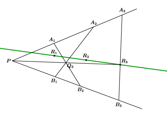
diagram 4. Leisenring’s theorem

If $\left\langle\begin{array}[]{ccc}A_{1}&A_{2}&A_{3}\\ B_{1}&B_{2}&B_{3}\end{array}\right\rangle$ denotes the Leisenring line containing the $R_{i}$, then we have the further theorem due to Rigby that the six lines

$$\Psi_{\sigma}=\left\langle\begin{array}[]{ccc}A_{1}&A_{2}&A_{3}\\ B_{\sigma(1)}&B_{\sigma(2)}&B_{\sigma(3)}\end{array}\right\rangle,\quad\sigma\in\mathfrak{S}_{3}$$

are also concurrent in threes exactly as in Steiner’s theorem. The proofs may be found in [15]. We omit the diagram, since as a visual pattern it is no different from the one for Steiner’s theorem. Let

$$\text{leisen}(\Pi)=\left\{\left\{\Psi_{e},\Psi_{(1\,2\,3)},\Psi_{(1\,3\,2)}\right\},\left\{\Psi_{(1\,2)},\Psi_{(2\,3)},\Psi_{(1\,3)}\right\}\right\}.$$

Theorem 6.1.

Let $\text{sig}(\Pi)=[x,y]$. If $x\neq y$, then $\text{leisen}(\Pi)$ is a Pappus structure. Moreover, it is equivalent to the structure $\text{steiner}(\Pi)$ obtained from Steiner’s theorem.

Essentially the same theorem is proved in [15, §3] by synthetic methods. We will give an analytic proof in Section 7.8. In general,

$$[\Psi_{\sigma}:\sigma\in\mathfrak{S}_{3}]\quad\text{and}\quad[\Lambda_{\sigma}:\sigma\in\mathfrak{S}_{3}],$$

are entirely different lines, but there is an automorphism of $\mathbb{P}^{2}$ carrying the first sequence to the second. We will find an explicit matrix for it immediately after the proof.

7. Some computations

We have collected some of the more computational proofs in this section.

7.1. The ‘standard’ Pappus structure

For any constants $r$ and $s$ (different from $0,1$) construct a collection of points $C(r,s)=\{A_{1},\dots,B_{3}\}$ as follows. Choose coordinates $z_{1},z_{2},z_{3}$ in $\mathbb{P}^{2}$, and let $L,M$ denote the lines $z_{1}=0,z_{2}=0$ respectively. Then $P=[0,0,1]$ is their point of intersection. The points

$$\begin{array}[]{lll}A_{1}=[0,1,r],&A_{2}=[0,1,1],&A_{3}=[0,1,0],\\ B_{1}=[1,0,s],&B_{2}=[1,0,1],&B_{3}=[1,0,0]\end{array}$$ (7.1)

are such that $\langle A_{1},A_{2},A_{3},P\rangle=r$, and $\langle B_{1},B_{2},B_{3},P\rangle=s$. Let $\Pi(r,s)$ denote the Pappus structure determined by $C(r,s)$. It will prove useful in many of the computations below.

If $N$ is a nonsingular $3\times 3$ matrix, define an automorphism $\varphi_{N}:\mathbb{P}^{2}\longrightarrow\mathbb{P}^{2}$ by sending the row-vector $[z_{1}\;z_{2}\;z_{3}]$ to $[z_{1}\;z_{2}\;z_{3}]\,N$.

7.2. Proof of Proposition 2.3

Write $r\sim r^{\prime}$, if $r^{\prime}$ is any of the functions of $r$ in (1.1).

Lemma 7.1.

Assume that $r\sim r^{\prime}$ and $s\sim s^{\prime}$. Then $\Pi(r,s)$ is isomorphic to $\Pi(r^{\prime},s^{\prime})$.

Proof.

We want to find an automorphism $\varphi_{N}$ of $\mathbb{P}^{2}$ which takes $\Pi(r,s)$ to $\Pi(r^{\prime},s^{\prime})$. Let $N=\left[\begin{array}[]{ccc}a&0&b\\ 0&c&d\\ 0&0&1\end{array}\right]$ for some $a,b,c,d$. Now it is easy to see that $\varphi_{N}$ preserves the lines $L$ and $M$, and hence also the point $P$. The image of a point on $L$ (resp. $M$) depends only on $c,d$ (resp. $a,b$). The gist of the lemma is that, depending on $r^{\prime}$ and $s^{\prime}$, we can independently specify the images of $A_{1},A_{2},B_{1},B_{2}$ under $\varphi_{N}$ by choosing $a,\dots,d$ correctly. Then the standard properties of the cross-ratio will ensure that $A_{3}$ and $B_{3}$ automatically land where we want them to.

For instance, let $r=1/(1-r^{\prime})$ and write $A_{1}^{\prime}=[0,1,r^{\prime}]$. Now $\langle A_{1}^{\prime},A_{2},A_{3},P\rangle=r^{\prime}$ implies that $\langle A_{3},A_{1}^{\prime},A_{2},P\rangle=r$. If we can arrange the entries in $N$ such that $\varphi_{N}$ takes $A_{1},A_{2}$ respectively to $A_{3},A_{1}^{\prime}$, then it will necessarily take $A_{3}$ to $A_{2}$. But this amounts to choosing $c,d$ such that $d+r=0,1+d=c\,r^{\prime}$, which can surely be done. Parallely, choose $a,b$ depending on $s^{\prime}$. All the other cases are very similar, and we leave them to the reader. ∎

Given a Pappus structure, we can always choose coordinates in the plane such that it is of the form $\Pi(r,s)$ for some $r,s$. Moreover, $\Pi(r_{1},s_{1})$ and $\Pi(r_{2},s_{2})$ have the same signatures, if and only if, either $r_{1}\sim r_{2},s_{1}\sim s_{2}$ or $r_{1}\sim s_{2},s_{1}\sim r_{2}$. This proves Proposition 2.3. ∎

7.3. Proof of Theorem 2.4

All the computations below were done in Maple, and it is a pleasant surprise that several intermediate expressions turn out to have clean and tidy factorisations. For the sake of brevity, we will give only the salient steps in the proof.

Starting from the standard Pappus structure, it is straightforward to calculate the coordinates of all Pappus lines. Let $E$ (resp. $E^{\prime}$) denote the point of concurrency of all even (resp. odd) lines. Their coordinates are

$$E =[r(r-1)(s^{2}-s+1),s\,(s-1)\,(r^{2}-r+1),rs(rs-1)],$$

$$E^{\prime} =[r(r-1)(s^{2}-s+1),-s(s-1)(r^{2}-r+1),rs(r-s)].$$

Either of these points is not well-defined, if all three lines passing through it coincide. We claim that at least one of these points is not defined, if and only if

$$r^{2}-r+1=0\quad\text{and}\quad s^{2}-s+1=0.$$ (7.2)

The ‘only if’ part is clear. For the converse, if $r,s$ are the roots of $Z^{2}-Z+1=0$, then either they are equal (when $E^{\prime}$ is undefined) or they are reciprocals (when $E$ is undefined). Henceforth we can assume that condition (7.2) is not satisfied. Then the two points are defined and turn out to be always distinct. Let $\Lambda_{*}$ denote the line joining them, and calculate the cross-ratios

$$c=\langle\Lambda_{e},\Lambda_{(1\,2\,3)},\Lambda_{(1\,3\,2)},\Lambda_{*}\rangle,\qquad c^{\prime}=\langle\Lambda_{(12)},\Lambda_{(1\,3)},\Lambda_{(2\,3)},\Lambda_{*}\rangle.$$

We will omit the expressions for $c$ and $c^{\prime}$, but write down their $j$-functions instead. Let

$$u =4\,(r^{2}-r+1)^{3}\,(s^{2}-s+1)^{3},$$

$$v =(rs-2r+s+1)(rs+r-2s+1)(2rs-r-s+2),$$

$$v^{\prime} =(rs+r+s-2)(2rs-r-s-1)(rs-2r-2s+1).$$

Then $j(c)=u/v^{2}$ and $j(c^{\prime})=u/v^{\prime 2}$. These are well-defined, if and only if $v,v^{\prime}$ are both nonzero. Now we have

$$x-y=j(r)+j(s)-j(r)\,j(s)=\frac{-4\,v\,v^{\prime}}{[27\,r(r-1)s(s-1)]^{2}},$$

so this happens exactly when $x\neq y$.

Let $\text{sig}(\text{steiner}(\Pi))=[p,q]$, which leads to equations

$$j(r)+j(s)-x=0,\quad j(r)\,j(s)-y=0,\quad j(c)+j(c^{\prime})-p=0,\quad j(c)\,j(c^{\prime})-q=0.$$

We should like to find $p,q$ in terms of $x,y$. Now consider the polynomial ring in variables $x,y,p,q,r,s$, with an elimination order with respect to the last two variables, and find the Gröbner basis of the ideal generated by the numerators of these equations. Then $r$ and $s$ get eliminated, leading to

$$2y\,(y-x+2)-p\,(x-y)^{2}=0,\quad\text{and}\quad y^{2}-q\,(x-y)^{2}=0.$$

This gives the required formula for the Pappus-Steiner map. The expressions show, once again, that $p,q$ are defined only when $x\neq y$. ∎

We can identify $\mathbb{P}^{1}$ with the pencil of lines through $P=[0,0,1]$, by sending $t$ to the line $z_{1}+t\,z_{2}=0$. Then the four lines $L,M,PE^{\prime},PE$ respectively correspond to the $t$-values

$$0,\quad\infty,\quad\pm\frac{r(r-1)(s^{2}-s+1)}{s(s-1)(r^{2}-r+1)},$$

leading to a cross-ratio of $-1$. In other words, the line-pair $PE,PE^{\prime}$ harmonically separates the line pair $L,M$. This was proved by Rigby in [15, §4] using synthetic methods.

7.4. Class field theory

In this section, we recall the bare essentials of class field theory which would suffice to prove Theorems 4.2 and 4.3. A comprehensive treatment of this subject may be found in [11]. The article by Lenstra and Stevenhagen [12] contains an engaging discussion of the Frobenius map and its relation to the Artin symbol. The computations below were done in Sage and confirmed in Maple.

Consider the polynomial

$$u(x)=x^{3}-84x^{2}+896x-1984,$$

from Section 4.2. Let $K$ denote the splitting field of $u(x)$, with discriminant $\Delta=2^{12}\,13^{2}\,31^{2}$ and $G=\text{Gal}(K/\mathbb{Q})\simeq C_{3}$. For every prime number $p$ not dividing $\Delta$, we have an Artin symbol $\varphi_{p}=\left[\frac{K/\mathbb{Q}}{p}\right]\in G$. If $u(x)$ factors in $\mathbb{F}_{p}$ as

$$u(x)=u_{1}(x)\,u_{2}(x)\dots u_{r}(x),$$

then each $u_{i}$ has the same degree, and moreover it equals the order of $\varphi_{p}$ in $G$. Hence $u(x)$ has a root in $\mathbb{F}_{p}$, exactly when $\varphi_{p}$ is the identity element.

The Kronecker-Weber theorem implies that we can embed $K$ in a cyclotomic field $\mathbb{Q}(\zeta_{m})$. Finding such an $m$ systematically is not easy (this would involve calculating the conductor of the field extension), but we can take advantage of the fact that the prime factors of $m$ also divide $\Delta$. If we experiment with small integers made of prime divisors $2,13$ and $31$, then we find that $u(x)$ splits completely in $L=\mathbb{Q}(\zeta_{13})$. Thus we have field extensions $\mathbb{Q}\subseteq K\subseteq L$, and there is a surjection of Galois groups

$$\text{Gal}(L/\mathbb{Q})\stackrel{{\scriptstyle h}}{{\longrightarrow}}\text{Gal}(K/\mathbb{Q}),$$

which sends the Artin symbol $\psi_{p}=\left[\frac{L/\mathbb{Q}}{p}\right]$ to $\varphi_{p}$. Hence $\varphi_{p}=e\iff\psi_{p}\in\ker h$. Now $\text{Gal}(L/\mathbb{Q})$ is canonically isomorphic to the multiplicative group of units

$$\mathbb{Z}_{13}^{\times}=\{a\in\mathbb{Z}_{13}:(a,13)=1\}\simeq C_{12},$$

and $\psi_{p}$ acts on $L$ by $z\longrightarrow z^{p}$. Thus

$$\psi_{p}\in\ker h\iff\psi_{p}^{4}=e\iff p^{4}\equiv 1\;\;(\text{mod}\,13).$$

The last condition is equivalent to $p\equiv 1,5,8,12\;\;(\text{mod}\,13)$.

7.5.

To see this differently, we can express a root of $u(x)$ in terms of $\zeta=\zeta_{13}$. The actual splitting shows that if we write

$$\gamma=1-\zeta^{2}-\zeta^{3}-\zeta^{10}-\zeta^{11}\quad\text{and}\quad\delta=\zeta^{4}+\zeta^{6}+\zeta^{7}+\zeta^{9},$$

then $\theta=20\,\gamma-4\,\delta$ is a root of $u(x)$, and $K=\mathbb{Q}(\theta)$. The characteristic property of the Artin symbol is that

$$\varphi_{p}(z)\equiv z^{p}\;\;(\text{mod}\,p),\quad\text{for any $z\in K$};$$

that is to say, it imitates the Frobenius map modulo $p$. Now $\varphi_{p}$ is the identity element if and only if it acts trivially on $\theta$, i.e., exactly when $\theta^{p}\equiv\theta\;\;(\text{mod}\,p)$. By the freshman’s dream,

$$\theta^{p}\equiv 20\,(1-\zeta^{2p}-\zeta^{3p}-\zeta^{10p}-\zeta^{11p})-4\,(\zeta^{4p}+\zeta^{6p}+\zeta^{7p}+\zeta^{9p}),$$

and hence this is tantamount to requiring that multiplication by $p$ should stabilise the sets $\{2,3,10,11\}$ and $\{4,6,7,9\}$ modulo $13$. It is easy to check that this happens exactly when $p\equiv 1,5,8,12$. For instance, if $p\equiv 5$, then

$$\{2,3,10,11\}\times 5=\{10,15,50,55\}\equiv\{10,2,11,3\}\;\;(\text{mod}\,13).$$

7.6.

The other two cases are similar. The cubic polynomial $v(x)=x^{3}-48x^{2}+656x-1856$ splits completely in $\mathbb{Q}(\zeta_{7})$, and we are reduced to finding the kernel of the surjection $\mathbb{Z}_{7}^{\times}\simeq C_{6}\longrightarrow C_{3}$. These are precisely the elements whose square is the identity, and hence

$$\text{$v(x)$ splits in $\mathbb{F}_{p}$}\iff p^{2}\equiv 1\;\;(\text{mod}\,7)\iff p\equiv 1,6\;\;(\text{mod}\,7).$$

The quartic polynomial $w(x)=x^{4}-144x^{3}+3152x^{2}-16896x+25856$ splits completely in $\mathbb{Q}(\zeta_{17})$, and we are reduced to finding the kernel of $\mathbb{Z}_{17}^{\times}\simeq C_{16}\longrightarrow C_{4}$. Thus,

$$\text{$w(x)$ splits in $\mathbb{F}_{p}$}\iff p^{4}\equiv 1\;\;(\text{mod}\,17)\iff p\equiv 1,4,13,16\;\;(\text{mod}\,17).$$

This completes the proofs of Theorems 4.2 and 4.3. ∎

The criteria in either theorem are inapplicable for finitely many primes. For instance, in Theorem 4.2 we must exclude the primes $2,13,31$, as well as those primes $p$ for which $\{f_{1},f_{2},f_{3}\}$ is not a Gröbner basis of $I_{3}$ modulo $p$. It would be possible to cover these exceptions by a tedious case-by-case computation, but this is unlikely to be of much interest.

7.7. Proof of Theorem 5.1

The theorem follows from some straightforward but elaborate computations, which were done in Maple. Once again, we will write down only the essential steps.

Following the definition of the point $P_{q}(t)$, its coordinates are found to be

$$[28\,q\,t^{2}-148\,q\,t+\dots+60,\;-16\,q\,t^{2}+\dots+64\,t,\;14\,q\,t^{2}+\dots+4\,t],$$

where we have omitted some intermediate terms for brevity. We are searching for a conic $\mathcal{C}_{q}$ which remains invariant under the map $\tau$. Now find the coordinates of $P^{\prime}=\tau(P)$ and calculate the expression

$$f(q,t)=\langle P^{\prime}R_{1},P^{\prime}R_{2},P^{\prime}R_{3},P^{\prime}R_{4}\rangle.$$

(It is too bulky to be written down in full.) If $\tau(\mathcal{C}_{q})=\mathcal{C}_{q}$, then we must have $f(q,t)=q$ regardless of the value of $t$. Hence we solve the equation $\frac{\partial f(q,t)}{\partial t}\equiv 0$. The derivative factors nicely, and we get a unique solution $q=2/7$. After back-substitution, we find that $f(2/7,t)=2/7$ as required. Hence $\tau(\mathcal{C}_{2/7})=\mathcal{C}_{2/7}$.

Now find the point $Q=\pi(P_{2/7}(t))$, and calculate the cross-ratio $\langle QR_{1},QR_{2},QR_{3},QR_{4}\rangle$. After some simplification, it turns out to be identically equal to $-1/4$. This shows that $\pi(\mathcal{C}_{2/7})=\mathcal{C}_{-1/4}$. Finally, the formulae for $\imath(t)$ and $\beta(t)$ are determined by the identities

$$L_{\imath(t)}=P^{\prime}R_{1},\quad L_{\beta(t)}=QR_{1}.$$

This completes the proof. ∎

As mentioned earlier, the entire calculation is speculative in the sense that a solution is by no means guaranteed a priori. But fortunately we do get a unique solution with very appealing properties.

7.8. Proof of Theorem 6.1

Let $F$ (resp. $F^{\prime}$) be the point of intersection of the line triple coming from even (resp. odd) permutations. Their coordinates are

$$F =[r(r-1)(s^{2}-s+1),s(s-1)(r^{2}-r+1),(r-1)(s-1)(r+s)(rs-1)],$$

$$F^{\prime} =[r(r-1)(s^{2}-s+1),-s(s-1)(r^{2}-r+1),-(r-1)(s-1)(rs+1)(r-s)].$$

These points are different from the $E$ and $E^{\prime}$ of Section 7.3, but essentially the same argument shows that $F$ and $F^{\prime}$ are both defined and distinct, if and only if either $r$ or $s$ is not a root of $Z^{2}-Z+1=0$. Let $\Psi_{*}=FF^{\prime}$, and now find the cross-ratios

$$d=\langle\Psi_{e},\Psi_{(1\,2\,3)},\Psi_{(1\,3\,2)},\Psi_{*}\rangle,\qquad d^{\prime}=\langle\Psi_{(12)},\Psi_{(1\,3)},\Psi_{(2\,3)},\Psi_{*}\rangle.$$

A direct calculation shows that $c=d$ and $c^{\prime}=d^{\prime}$, hence $\text{leisen}(\Pi)$ is equivalent to $\text{steiner}(\Pi)$. ∎

Thus we must have an automorphism $\varphi_{N}$ of $\mathbb{P}^{2}$ such that $\varphi_{N}(\Lambda_{\sigma})=\Psi_{\sigma}$ for all $\sigma$ in $\mathfrak{S}_{3}\cup\{*\}$. Since we know the coordinates of all the fourteen lines, we can find its matrix by solving a system of linear equations. The answer comes out to be $N=\left[\begin{array}[]{ccc}2&0&s+1\\ 0&2&r+1\\ 0&0&-1\end{array}\right]$. Notice that $\varphi_{N}$ preserves the lines $z_{1}=0,z_{2}=0$. Hence, it slides the points $A_{1},\dots,B_{3}$ along the same lines into new positions $\widetilde{A}_{1},\dots,\widetilde{B}_{3}$, like beads woven on a wire, in such a way that

$$\text{Pappus lines of $A_{1},\dots,B_{3}$}=\text{Leisenring lines of $\widetilde{A}_{1},\dots,\widetilde{B}_{3}$}.$$

This is shown schematically in Diagram 5.

diagram 5. The drawing is not intended to be geometrically accurate. The actual Pappus lines are not the ones shown.

7.9.

Recall the involutive operation $r\rightarrow r^{\circ}$ from Section 3.4. Although $\Pi(r,s)$ and $\Pi(r^{\circ},s^{\circ})$ are in general inequivalent Pappus structures, we have

$$\text{sig}(\text{steiner}(\Pi(r,s))=\text{sig}(\text{steiner}(\Pi(r^{\circ},s^{\circ})).$$

In other words, the two sequences of points $C(r,s)$ and $C(r^{\circ},s^{\circ})$ lead to projectively equivalent sextuples of Pappus lines. Exactly as in the previous section, we can find the matrix $T$ whose associated automorphism $\varphi_{T}$ takes the first sextuple to the second. The answer comes out to be

$$T=\left[\begin{array}[]{ccc}\frac{(2s-1)(s-2)}{s(s-1)}&0&\frac{s-2}{s-1}\\ 0&\frac{(2r-1)(r-2)}{r(r-1)}&\frac{r-2}{r-1}\\ 0&0&-3\end{array}\right].$$

Once again, it is easy to see that $\varphi_{T}$ preserves the lines $z_{1}=0,z_{2}=0$. Said differently, we have two distinct sequences of points, namely $\varphi_{T}(C(r,s))$ and $C(r^{\circ},s^{\circ})$, supported on the same pair of lines, which lead to the same sextuple of Pappus lines. It would be interesting to have a synthetic proof of this result.

8. Appendix: The Pappus-Steiner map over real numbers

by Attila Dénes

This section contains a short computer-aided analysis of the Pappus-Steiner map (2.3) over the field $k=\mathbb{R}$. In order to study its dynamical behaviour, we used the computer program developed by Dénes and Makay [5], which helps in the visualisation of attractors and basins of dynamical systems.

According to the algorithm given in [5], if an orbit leaves some multiple of the area under examination, then we assume that this orbit diverges. However, such a judgment must always be tentative, since such an orbit may return several steps later. If one calculates some orbits of the Pappus–Steiner map, then one can see examples of orbits getting very far from the origin and still returning close to it after some iterations. The results obtained suggest that $(0,0)$ is an attractor of the system (see Diagram 6), although the map itself is undefined at this point. It is generally difficult to handle these orbits numerically, since the coordinates of the points become very small near the origin.

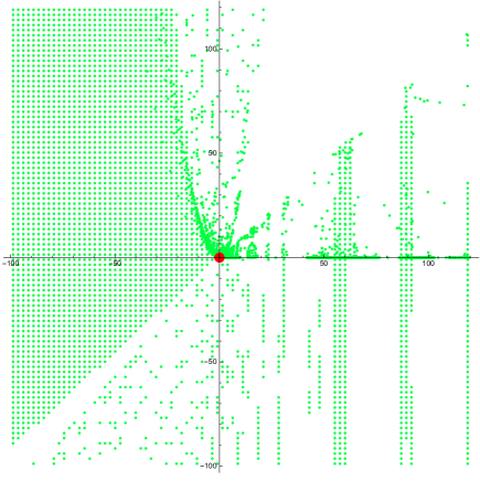
diagram 6. The origin as attractor (shown in red) and its basin (shown in green)

There are also orbits which tend to an attractor consisting of the two points $(0,0)$ and $(1,0)$. Although the possibility of numerical errors also holds for these orbits, one may support the conjecture of the existence of such an attractor by considering a point $(1+\varepsilon,\delta)$ close to $(1,0)$, whose first iterate

$$\left(\frac{2\delta(\delta-(1+\varepsilon)+2)}{(1+\varepsilon-\delta)^{2}},\frac{\delta^{2}}{(1+\varepsilon-\delta)^{2}}\right)\approx(2\delta,\delta^{2})$$

is close to $(0,0)$, while iterating $(2\delta,\delta^{2})$ gives

$$\left(\frac{2\delta^{2}(\delta^{2}-2\delta+2)}{(2\delta-\delta^{2})^{2}},\frac{\delta^{4}}{(2\delta-\delta^{2})^{2}}\right)\approx\left(1-\delta,\frac{\delta^{2}}{4}\right)$$

which is again close to $(1,0)$. This argument also suggests asymptotic stability of this attractor, because if $\delta$ is small, then $\delta^{2}/4$ is even smaller. One can also obtain similar attractors formally, e.g., $\left\{(0,0),(4,0)\right\}$. Diagram 7 suggests that there might be other attractors consisting of several points.

diagram 7. Attractor (shown in red) including the origin and points of the $x$ axis and its basin (shown in blue)

The most interesting region is the one between the line $y=x-1$ of harmonic structures, and the parabola $4y=x^{2}$ of balanced structures (see Diagram 8). Numerical experiments suggest that there are points whose orbits are dense in this region. However this statement must again be taken with some degree of caution, since the expression for $\pi$ becomes numerically unstable near the line $x=y$.

diagram 8. The region between the harmonic line and the balanced parabola

Acknowledgement: The first author is thankful to Siddarth Sankaran for his help with the number-theoretic calculations in Sections 7.4 through 7.6.

–

References

- [1] Adams, W. and Loustaunau, P. An Introduction to Gröbner Bases. Graduate Studies in Mathematics, vol. 3. American Mathematical Society, 1994.
- [2] Baker, H. F. Principles of Geometry, vol. II. Cambridge University Press, 1923.
- [3] Beardon, A. Iteration of Rational Functions. Graduate Texts in Mathematics, vol. 132. Springer-Verlag, New York, 1991.
- [4] Coxeter, H. S. M. Projective Geometry. Springer-Verlag, New York, 1994.
- [5] Dénes, A. and Makay, G. Attractors and basins of dynamical systems. Electron. J. Qual. Theory Differ. Equ., no. 20, 11 pp., 2011.
- [6] Devaney, R. An Introduction to Chaotic Dynamical Systems. The Benjamin/Cummings Publishing Co., 1986.
- [7] Hooper, P. W. From Pappus’ theorem to the twisted cubic. Geom. Dedicata, vol. 110, pp. 103–134, 2005.
- [8] Hulpke, A. Techniques for the computation of Galois groups, In Algorithmic algebra and number theory (Heidelberg, 1997), pp. 65–77, Springer, Berlin, 1999.
- [9] Ireland, K. and Rosen, M. A Classical Introduction to Modern Number Theory. Graduate Texts in Mathematics, Springer-Verlag, New York, 1990.
- [10] Kadison, L. and Kromann, M. T. Projective Geometry and Modern Algebra. Birkhäuser, Boston, 1996.
- [11] Lang, S. Algebraic Number Theory. Graduate Texts in Mathematics, Springer-Verlag, New York, 1994.
- [12] Lenstra, H. W., Jr. and Stevenhagen, P. Artin reciprocity and Mersenne primes. Nieuw Arch. Wiskd. vol. 5, no. 1, pp.44-54, 2000.
- [13] Milne, J. Algebraic Number Theory (v3.07). Available at ‘www.jmilne.org/math/’, (165 pages), 2017.
- [14] Milnor, J. Geometry and dynamics of quadratic rational maps (with an appendix by the author and Lei Tan). Experiment. Math., vol. 2, no. 1, pp. 37–83, 1993.
- [15] Rigby, J. F. Pappus lines and Leisenring lines. J. Geom., vol. 21, no. 2, pp. 108–117, 1983.
- [16] Roblot, X.-F. Polynomial factorization algorithms over number fields. J. Symbolic Computation, vol. 38, no. 5, pp. 1429–1443, 2004.
- [17] Schwartz, R. Pappus’s theorem and the modular group, Inst. Hautes Études Sci. Publ. Math., vol. 78, pp. 187–206, 1994.
- [18] Seidenberg, A. Lectures in Projective Geometry. D. Van Nostrand Company, New York, 1962.
–
Jaydeep Chipalkatti
Department of Mathematics,
University of Manitoba,
Winnipeg, MB R3T 2N2.
Canada.
jaydeep.chipalkatti@umanitoba.ca
Attila Dénes
Bolyai Institute,
University of Szeged,
Aradi vértanúk tere 1,
H-6720, Szeged, Hungary.
denesa@math.u-szeged.hu