First-passage dynamics of linear stochastic interface models:
numerical simulations and entropic repulsion effect

Abstract

A fluctuating interfacial profile in one dimension is studied via Langevin simulations of the Edwards-Wilkinson equation with non-conserved noise and the Mullins-Herring equation with conserved noise. The profile is subject to either periodic or Dirichlet (no-flux) boundary conditions. We determine the noise-driven time-evolution of the profile between an initially flat configuration and the instant at which the profile reaches a given height $M$ for the first time. The shape of the averaged profile agrees well with the prediction of weak-noise theory (WNT), which describes the most-likely trajectory to a fixed first-passage time. Furthermore, in agreement with WNT, on average the profile approaches the height $M$ algebraically in time, with an exponent that is essentially independent of the boundary conditions. However, the actual value of the dynamic exponent turns out to be significantly smaller than predicted by WNT. This “renormalization” of the exponent is explained in terms of the entropic repulsion exerted by the impenetrable boundary on the fluctuations of the profile around its most-likely path. The entropic repulsion mechanism is analyzed in detail for a single (fractional) Brownian walker, which describes the anomalous diffusion of a tagged monomer of the interface as it approaches the absorbing boundary. The present study sheds light on the accuracy and the limitations of the weak-noise approximation for the description of the full first-passage dynamics.

I Introduction

In the present study, first-passage events arising in the Edwards-Wilkinson and the Mullins-Herring equation for various boundary conditions are investigated based on Langevin simulations. The obtained results for the spatio-temporal evolution of the profile are confronted to WNT — which has been discussed in a preceding paper (Ref. Gross (2017)) — and to reduced models of (fractional) Brownian walkers. In order to make the present study self-contained, the relevant models are briefly reviewed in the following.

We consider a one-dimensional interfacial profile $h(x,t)$, defined on a domain of size $L$ ($0\leq x\leq L$) governed by either the Edwards-Wilkinson (EW) equation Edwards and Wilkinson (1982)

$$\partial_{t}h=\eta\partial_{x}^{2}h+\zeta\,,$$ (1)

or the stochastic Mullins-Herring (MH) equation Mullins (1957); Herring (1950); Krug (1997)

$$\partial_{t}h=-\eta\partial_{x}^{4}h+\partial_{x}\zeta.$$ (2)

The noise $\zeta$ is a Gaussian random variable of zero mean and correlation

$$\langle\zeta(x,t)\zeta(x^{\prime},t^{\prime})\rangle=2D\delta(x-x^{\prime})\delta(t-t^{\prime})\,.$$ (3)

The ratio between the friction coefficient $\eta$ and the noise strength $D$ is related to the temperature via a fluctuation-dissipation relation (see below). The initial configuration is generally taken to be flat,

$$h(x,t=0)=0,$$ (4)

and the profile is assumed to fulfill either periodic boundary conditions (p)

$$h^{\text{(p)}}(x,t)=h^{\text{(p)}}(x+L,t),$$ (5)

or Dirichlet boundary conditions (D)

$$h^{\text{(D)}}(0,t)=0=h^{\text{(D)}}(L,t).$$ (6)

When using the latter in conjunction with the MH equation, we additionally impose a no-flux condition at the boundaries,

$$\partial_{x}^{3}h^{(\mathrm{D}^{\prime})}(0,t)=0=\partial_{x}^{3}h^{(\mathrm{D}^{\prime})}(L,t),$$ (7)

which is indicated by a primed superscript (D’). For the MH equation with periodic or Dirichlet no-flux boundary conditions, the area under $h$,

$$\mathcal{A}([h],t)\equiv\int_{0}^{L}\mathrm{d}x\,h(x,t)\,,$$ (8)

henceforth called the “mass”, is conserved in time:

$$\mathcal{A}([h],t)=0.$$ (9)

In contrast, due to the presence of $\zeta$ instead of $\partial_{x}\zeta$ in Eq. 1, the mass is generally not conserved for the EW equation. In particular, for periodic boundary conditions, $\mathcal{A}([h],t)$ behaves diffusively at large times Gross and Varnik (2013); Krug (1997), while for Dirichlet boundary conditions, $\langle\mathcal{A}([h],t)\rangle=0$ holds only as a time-average. In order to enforce Eq. 9 also for EW dynamics with periodic boundary conditions, we consider in this case instead of $h^{\text{(p)}}$ the profile

$$\tilde{h}^{\text{(p)}}(x,t)\equiv h^{\text{(p)}}(x,t)-\mathcal{A}([h^{\text{(p)}}],t)/L,\qquad\text{(EW)}$$ (10)

which fulfills $\mathcal{A}([\tilde{h}^{\text{(p)}}],t)=0$. In the simulations discussed here, the prescription in Eq. 10 is applied at each time step. In order to simplify notation, the tilde will be dropped henceforth. We emphasize that Eq. 10 is rather artificial from a physical point of view and is imposed here mainly in order to compare the different models under the common condition $\langle\mathcal{A}([h],t)\rangle=0$.

We focus on the stochastic evolution of $h(x,t)$ until the (random) first-passage time $T$, at which the profile has reached a given maximum height $M>0$ for the first time:

$$\max_{x}h(x,T)=M.$$ (11)

The resulting (random) coordinate $x$ will be denoted in the following by $x_{M}$. Equation 11 implies an absorbing boundary condition for the profile at the height $M$ Gardiner (2009); Redner (2001). The absorbing boundary condition acts over the whole domain $[0,L]$ and represents an impenetrable repulsive barrier to the profile (see also Refs. Delfino and Squarcini (2013); Belardinelli et al. (2016)). For a highly correlated system, such as an profile in the presence of a mass constraint [Eq. 9], analytical solutions of the first-passage problem are technically difficult and are available only in certain limits (see, e.g., Refs. Krug et al. (1997); Likthman and Marques (2006); Guerin et al. (2012); Bray et al. (2013); Cao et al. (2015); Meerson and Vilenkin (2016)). The first-passage dynamics of the profile is thus addressed here via numerical simulation of Eqs. 1 and 2, as well as by relying on reduced descriptions of the effective (fractional) Brownian dynamics of a “tagged monomer”, i.e., of $h(x_{M},t)$. Note that, in the absence of an absorbing boundary, the stochastic process governed by Eqs. 1 and 2 is fully Gaussian and underlies the well-studied phenomenon of interfacial roughening (see, e.g., Refs. Krug (1997); Halpin-Healy and Zhang (1995) as well as Appendix F).

A tractable approximation to the first-passage problem discussed here is provided by weak-noise theory (WNT), also known as macroscopic fluctuation theory Freidlin and Wentzell (1998); Bertini et al. (2015); Meerson and Vilenkin (2016). WNT of Eqs. 1 and 2 has been discussed in detail in Ref. Gross (2017). WNT represents a leading-order saddle-point approximation to the first-passage problem and describes the most-likely (“optimal”) trajectory between two states. Specifically, within WNT, Eq. 11 is replaced by a height constraint, $h(x,T)=M$, and the first-passage time $T$ is taken as a free, but constant, parameter. Accordingly, WNT neither takes into account fluctuation-induced interactions with the absorbing boundary nor the fact that the first-passage time $T$ follows a certain probability distribution. However, it is shown here that, despite these limitations, WNT accurately captures the scaling functions of the averaged profile shape. A significant difference nevertheless arises in the value of the dynamic exponent characterizing the time-dependence of the first-passage profile. Based on insights from models of (fractional) Brownian walkers, this difference is argued to be a genuine consequence of the fluctuations around the most-likely path near an impenetrable boundary.

The first-passage problem of the MH equation discussed here and in Ref. Gross (2017) is, inter alia, physically relevant for noise-driven rupture of liquid films on substrates. So far, typically films have been considered which are either linearly unstable with respect to small fluctuations of the interface or where the rupture proceeds via hole nucleation in the presence of disjoining pressure Bausch and Blossey (1994); Bausch et al. (1994); Blossey (1995); Foltin et al. (1997); Seemann et al. (2001); Thiele et al. (2001, 2002); Tsui et al. (2003); Becker et al. (2003); Gruen et al. (2006); Fetzer et al. (2007); Croll and Dalnoki-Veress (2010); Blossey (2012); Nguyen et al. (2014); Duran-Olivencia et al. (2017). Here and in Ref. Gross (2017), we focus on linearized models in one dimension and assume absence of any deterministic force beside surface tension. In particular, we neglect the influence of disjoining pressure, which is experimentally justified for colloidal fluids Lekkerkerker et al. (2008); Aarts and Lekkerkerker (2008). Accordingly, in this case film rupture is solely driven by noise. This situation is analogous to the noise-driven breakup of a liquid nanojet, which has been analyzed within WNT in Ref. Eggers (2002) and studied experimentally and by simulations in Refs. Petit et al. (2012); Hennequin et al. (2006); Mo et al. (2015). Physical realizations of one-dimensional interfaces occur, e.g., in lipid bilayer membranes below their demixing transition Honerkamp-Smith et al. (2008); Thiam et al. (2013). The extension of the present study to two-dimensional interfaces as well as the incorporation of an interface potential are reserved for future work.

II Model and simulations

II.1 General aspects

In the following, a number of relevant properties of the considered models are summarized. It is useful to note that, dimensionally $[\eta]\sim[L]^{z}/[T]$, $[D]\sim[M]^{2}[L]^{z-1}/[T]$, $[D/\eta]=[M]^{2}/[L]$, where $[M]$, $[L]$, and $[T]$ represent the fundamental dimensions of height, length, and time, respectively. In order to facilitate the analysis of the first-passage dynamics, we recall the phenomenology of interfacial roughening (see Appendix F for details). To this end, we consider Eqs. (1) and (2) in the absence of an absorbing boundary condition. In this situation, one can analytically determine the trajectory $h(x,t)$ as well as the roughness $\langle|\delta h(x,t)|^{2}\rangle$, where $\delta h(x,t)\equiv h(x,t)-h(x,0)$ is the relative height fluctuation. We consider either a flat initial condition, $h(x,0)=0$, or a thermal one. In the latter case, the roughness is calculated as an average over an ensemble of equilibrium profiles $h(x,0)$. Since, for Dirichlet boundary conditions, the variance depends on position, we evaluate in the following $\langle h(x,t)\rangle$ at a fixed location $x_{M}$ far from the boundaries (the precise value of $x_{M}$, however, is irrelevant for the general scaling behavior). The roughness resulting from Eqs. 1 and 2 is characterized by three regimes Majaniemi et al. (1996); Abraham and Upton (1989); Racz et al. (1991); Antal and Racz (1996); Barabasi and Stanley (1995); Majaniemi et al. (1996); Flekkoy and Rothman (1995, 1996); Krug (1997); Taloni et al. (2010a, 2012, b); Panja (2011); Gross and Varnik (2013); Halpin-Healy and Zhang (1995):

$$\langle|\delta h(x_{M},t)|^{2}\rangle\sim\begin{cases}t,\quad&t\lesssim\tau_{\times},\\ t^{1/z},&\tau_{\times}\lesssim t\lesssim\tau,\\ \mathrm{const},&t\gtrsim\tau,\end{cases}$$ (12)

where

$$z\equiv\begin{cases}2,\qquad\text{EW equation},\\ 4,\qquad\text{MH equation},\end{cases}$$ (13)

is the dynamic index and $\tau$ denotes the roughening time. The latter coincides with the relaxation time of the (eigen-)mode with the largest “wavelength” that can be accommodated in the system:

$$\tau=\left(\frac{L}{\omega_{1}}\right)^{z},\qquad\omega_{1}\equiv\begin{cases}2\pi,\qquad&\text{periodic,}\\ \pi,\qquad&\text{standard Dirichlet,}\\ 4.73\ldots\qquad&\text{Dirichlet no flux boundary conditions.}\end{cases}$$ (14)

Dirichlet no-flux boundary conditions are considered only for the MH equation ($z=4$), in which case the value $\omega_{1}\simeq 4.73$ represents the smallest positive solution of the associated eigenvalue equation, $\cos\omega\cosh\omega=1$ [see Appendix E]. Within WNT, $\tau$ is in fact the characteristic time scale for the development of the first-passage profile in an equilibrium system (see Ref. Gross (2017)). This property is confirmed by the present simulations. Furthermore, $\tau_{\times}$ in Eq. 12 represents a cross-over time related to the presence of a microscopic cutoff. While $\tau_{\times}=0$ in the continuum limit, for a one-dimensional lattice one has (see Appendix G)

$$\tau_{\times}=\tau\left(\frac{\omega_{1}}{\omega_{k_{\times}}}\right)^{z},$$ (15)

with $\omega_{k_{\times}}^{\text{(p)}}=2L/\Delta x$ and $\omega_{k_{\times}}^{\text{(D)}}=L/\Delta x$ for periodic and (standard) Dirichlet boundary conditions, respectively, where $\Delta x$ is the lattice spacing. For Dirichlet no-flux boundary conditions, a numerical analysis yields $k_{\times}\gtrsim 0.5L/\Delta x$, with the actual value depending on the particular problem under study [see Section G.2; the corresponding value of $\omega^{(\mathrm{D}^{\prime})}_{k_{\times}}$ follows from the eigenvalue equation in Eq. 110].

According to Eq. 12, a tagged monomer of the profile exhibits standard Brownian diffusion at early times, followed by a subdiffusive regime characterized by a Hurst exponent Family and Vicsek (1991); Meakin (1993)

$$H=\frac{1}{2z}.$$ (16)

For a sufficiently large system, the latter regime dominates the roughening behavior. A tagged monomer thus diffuses the distance $M$ approximately within the time [see Eq. 140]

$$\tau_{D}=\frac{M^{1/H}}{2[(2/\pi)\Theta\Gamma(1-z^{-1})]^{z}\eta},$$ (17)

where $\Theta$ is the temperature [see Eq. 19 below]. The numerical prefactors in Eq. 17 arise from a detailed analysis (see Appendix F) along with the two-time correlation function of the relative height fluctuations $\delta h(x,t)$ [see Eq. 138],

$$\langle\delta h(x,t)\delta h(x,s)^{*}\rangle_{\text{flat}} \simeq(2/\pi)\eta^{1/z}\Gamma(1-z^{-1})\Theta\left[(t+s)^{1/z}-|t-s|^{1/z}\right],$$ (18a)

$$\langle\delta h(x,t)\delta h(x,s)^{*}\rangle_{\text{th}} \simeq(2/\pi)\eta^{1/z}\Gamma(1-z^{-1})\Theta\left[t^{1/z}+s^{1/z}-|t-s|^{1/z}\right],$$ (18b)

corresponding to flat and thermal initial conditions, respectively. The Gaussian stochastic process described by Eq. 18b is a fractional Brownian motion (fBM) Kolmogoroff (1940); Mandelbrot and Van Ness (1968); McCauley et al. (2007); Jeon and Metzler (2010) .

For times $t\gtrsim\mathcal{O}(\tau)$, all memory of the initial condition has been lost and the interface has reached its equilibrium roughness. In this regime, the profile $h(x,t)$ follows a time-independent joint Gaussian distribution with a temperature (see Appendix B)

$$\Theta=\frac{D}{2\eta}.$$ (19)

This equation represents a fluctuation-dissipation relation for Eqs. 1 and 2. For periodic boundary conditions, the one-point variance $\langle h(x,t)^{2}\rangle$ is independent of position $x$ and is in equilibrium given by [see Eq. 61]

$$\langle|h^{\text{(p)}}|^{2}\rangle=\frac{1}{6}\Theta L.$$ (20)

For Dirichlet boundary conditions, the equilibrium variance at the mid-point $x=L/2$ is given by [see Eqs. 64 and 66]

$$\langle[h^{\text{(D)}}(L/2,t)])^{2}\rangle =\frac{1}{2}\Theta L$$ (21a)

and

$$\langle[h^{(\mathrm{D}^{\prime})}(L/2,t)]^{2}\rangle =\frac{7}{8}\Theta L,$$ (21b)

in the cases without and with an additional mass constraint [Eq. 9], respectively.

The first-passage dynamics is generally distinct in the transient and the equilibrium regime, which, within WNT, correspond to $T/\tau\ll 1$ and $T/\tau\gg 1$, respectively. However, for the actual stochastic equations (1) and (2), the first-passage time $T$ is a random quantity and $T/\tau$ is therefore not an appropriate parameter . We thus define instead the reduced height

$$\mathcal{M}\equiv\frac{M}{\sqrt{\Theta L}}\sim\frac{M}{\langle h^{2}\rangle^{1/2}},$$ (22)

which is essentially the ratio between the maximum height $M$ and the equilibrium variance of the profile [Eqs. 20 and 21]. For $\mathcal{M}\ll 1$, the profile is likely to reach the height $M$ within its roughening phase, whereas for $\mathcal{M}\gg 1$, the profile is fully equilibrated before the first-passage event occurs. The definition in Eq. 22 is consistent with the fact that the transient regime corresponds to diffusion times $\tau_{D}\ll\tau$ [see Eqs. 17 and 14]. We henceforth take $\tau_{D}$ and $\tau$ as the fundamental time scales for the first-passage dynamics in the transient and equilibrium regimes, respectively.

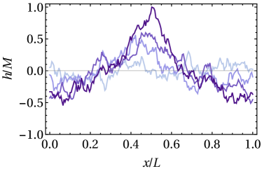
Figure 1: Typical time evolution of a profile $h(x,t)$ until the first-passage event (time $T$), at which the height $M$ is reached for the first time [see Eq. 11]. The plotted profiles represent snapshots at times $(T-t)/\tau^{\text{(p)}}\simeq 0.5,0.05,0.02,5\times 10^{-5}$ (from center bottom to top) obtained from a simulation of Eq. 1 for periodic boundary conditions [and with Eq. 10 imposed at each time step] on a lattice size of $L=200\Delta x$. $\tau^{\text{(p)}}$ denotes the fundamental relaxation time reported in Eq. 14. The initial profile is flat [Eq. 4, not shown]. Owing to translational invariance in the case of periodic boundary conditions, the individual profiles are shifted such that the maximum occurs at the center of the box, i.e., $h(x_{M}=L/2,T)=M$.

II.2 Implementation

The stochastic equations in Eqs. 1 and 2 are discretized on a one-dimensional lattice comprising $N=L/\Delta x$ nodes with spacing $\Delta x$ and are solved using a standard forward Euler scheme with time step $\Delta t$ (see, e.g., Refs. Krug et al. (1997); Karma and Rappel (1999)):

$$h(x_{i},t+\Delta t)=h(x_{i},t)-\eta\,\Delta t\,(-\nabla^{2})^{z/2}h(x_{i},t)+\sqrt{2D\Delta t}\nabla^{z/2-1}\tilde{\zeta}(x_{i},t),$$ (23)

with $i=0,\ldots,N-1$. The noise variables $\tilde{\zeta}(x_{i})$ are uncorrelated Gaussian variables of zero mean and unit variance, $\langle\tilde{\zeta}(x_{i},t)\tilde{\zeta}(x_{j},t^{\prime})\rangle=\delta_{i,j}\delta_{t,t^{\prime}}$. The discretized forms of the derivative operators $\nabla^{2}$ and $\nabla^{4}$ as well as further technical details on the numerical simulations are provided in Appendix G. In the simulations, a profile is generally initialized in a flat configuration [Eq. 4]. If an equilibrated system is required at the first-passage event, the height $M$ is chosen sufficiently large such that $T\gg\tau$ (see also Section III). Figure 1 exemplifies a typical time evolution of a profile governed by Eq. 1 close to the first-passage event.

The main object of the present study is the averaged profile $\langle h(x,\delta t)\rangle$, which is obtained in the following way: let $\{h^{(s)}(x,t)\}$, $s=1,\ldots,S$ be an ensemble of profiles obtained from a total number of $S$ simulations. Let $T^{(s)}$ be the corresponding first-passage time, such that $h^{(s)}(x_{M}^{(s)},T^{(s)})\geq M$ for the first time for any $x_{M}^{(s)}$. The averaged profile is defined as

$$\langle h(x,\delta t)\rangle\equiv\frac{1}{N(T\geq\delta t)}\sum_{s=1}^{N(T\geq\delta t)}h^{(s)}(x-X^{(s)},T^{(s)}-\delta t),$$ (24)

where $N(T\geq\delta t)\leq S$ denotes the number of profiles for which $T^{(s)}\geq\delta t$. Note that the averaged profile is a function of the time variable $\delta t$, which is defined such that the first-passage event corresponds to $\delta t=0$, i.e., $\langle h(x_{M},0)\rangle=M$. Depending on the model and the regime considered, we set either $X^{(s)}\equiv 0$ or $X^{(s)}\equiv x^{(s)}_{M}-L/2$, where the latter choice induces a shift of the location of the maximum $x_{M}^{(s)}$ to the center $L/2$ .

The finite value of the time step in Eq. 23 gives rise to two potentials errors: first, a profile can “overshoot” the boundary, i.e., instead of Eq. 11 one finds $h^{(s)}(x_{M},T)=M+\delta M^{(s)}$ with $\delta M^{(s)}>0$. This effect is taken into account by subtracting the individual $\delta M^{(s)}$ on the r.h.s. of Eq. 24. While the overshoot leads to slight changes of the observed scaling of the peak $\langle h(x,\delta t)\rangle$ for small $\delta t$, it turns out to not significantly affect the intermediate asymptotics. Second, there is a certain finite probability that between two discrete time steps the profile has crossed the boundary Clifford and Green (1986); Peters and Barenbrug (2002). Performing simulations with a decreased time step in a few cases indicate that the results here are essentially insensitive to this effect.

III First-passage time

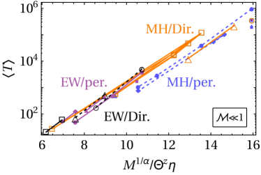
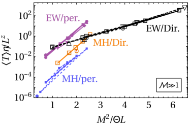
Figure 2: Mean first-passage time $\langle T\rangle$ for a profile with flat initial configuration [Eq. 4] in (a) the transient and (b) the equilibrium regime, corresponding to $\mathcal{M}\ll 1$ and $\mathcal{M}\gg 1$, respectively [see Eq. 22]. In (a), effective values $\alpha_{\text{EW}}=0.29$ and $\alpha_{\text{MH}}=0.17$ are used for the exponent $\alpha$ in the scaling relation (26). Time is expressed in units of the simulation time step $\Delta t$. In (b), the axes are scaled according to Eq. 27. The bulk dynamic equation and the boundary conditions are indicated by the labels near the data (purple solid symbols connected by solid lines: EW equation with periodic bc.s; black open symbols connected by dashed lines: EW equation with Dirichlet bc.s; blue solid symbols connected by dashed lines: MH equation with periodic bc.s; orange open symbols connected by solid lines: MH equation with Dirichlet no-flux bc.s).

Before addressing the profile dynamics, we briefly turn to the first-passage time $T$, i.e., the time at which the profile, starting from the initial configuration in Eq. 4, reaches the given height $M$ for the first time. We remark that related first-passage problems of linear interface and polymer models have been studied previously in, e.g., Refs. Krug et al. (1997); Kantor and Kardar (2007); Chatelain et al. (2008); Amitai et al. (2010); Bray et al. (2013). Closed analytical expressions are, however, available only within certain approximations Guerin et al. (2012); Cao et al. (2015); Likthman and Marques (2006).

The first-passage distribution $\mathcal{P}_{1}(T)$ is discussed separately in Appendix A. For the models considered here, we find that $\mathcal{P}_{1}(T)$ decays either exponentially or algebraically for large $T$, with an exponent smaller than $-2$. Consequently, the mean first-passage time

$$\langle T\rangle=\int_{0}^{\infty}\mathrm{d}T\,T\mathcal{P}_{1}(T)$$ (25)

is finite. In order to obtain an estimate for $\langle T\rangle$ in the transient regime, we recall that a tagged monomer traverses the distance between $h=0$ and $M$ within a time of order of $t^{\alpha}$, with $\alpha=1/(2z)$. Specifically, based on Eq. 17 one expects

$$\langle T\rangle\sim\frac{M^{1/\alpha}}{\Theta^{z}\eta}.$$ (26)

However, instead of the naive value $\alpha=1/(2z)$, we use in Eq. 26 the effective values $\alpha_{\text{EW}}\simeq 0.27-0.3$ and $\alpha_{\text{MH}}\simeq 0.16-0.18$ in the case of EW and MH dynamics, respectively, which coincide with the values of the exponent characterizing the averaged path (see Sections IV and V). As demonstrated in Fig. 2, the scaling behavior of the mean first-passage time in the transient regime is well captured by the scaling relation (26) .

In the equilibrium regime, Eq. 26 does not provide a satisfactory description of the mean first-passage time. Instead we recall that the steady-state probability distribution of the profile is Gaussian with a single-site variance given in Eqs. 20 and 21. We can thus consider a tagged monomer $h(x_{M},t)$ as a fractional Brownian walker [$H=1/(2z)<1/2$, see Eq. 18b] in an effective harmonic potential $U(h)\simeq h^{2}/\Theta L$. To leading order, the monomer dynamics can be approximated by a Markovian Brownian process ($H=1/2$), such that the present first-passage problem reduces to the well-known Kramers escape problem Gardiner (2009); Malakhov and Pankratov (1996). Accordingly, the mean-first-passage time of a tagged monomer in the equilibrium regime is expected to behave as

$$\langle T\rangle\simeq c_{1}L^{z}\eta^{-1}\exp\left(c_{2}\frac{M^{2}}{\Theta L}\right),$$ (27)

where $c_{1}$ and $c_{2}$ are fit parameters (independent of $M$, $L$ and $\Theta$) . Essentially the same form as in Eq. 27 has been obtained in Ref. Sliusarenko et al. (2010) for a fBM in a parabolic potential as well as in Ref. Cao et al. (2015) in the case of a Rouse polymer chain. As demonstrated in Fig. 2, the simulation data pertaining to each model falls onto distinct master curves described by Eq. 27.

IV Edwards-Wilkinson equation

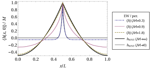
Figure 3: Averaged profile $\langle h(x,\delta t=0)\rangle$ (broken lines) at the first-passage event, as obtained from simulations of the EW equation [Eq. 1] with periodic boundary conditions and for various reduced heights $\mathcal{M}$ [Eq. 22]. A constraint of zero mass [Eq. 9] is imposed via Eq. 10. The solid lines represent the asymptotic scaling profiles predicted by WNT in the transient regime [$\mathcal{M}\to 0$, Eq. 28, sharply peaked curve] and in the equilibrium regime [$\mathcal{M}\to\infty$, Eq. 32a, broadly peaked curve]. In the former case, the parameter $T$ results from a fit as $T\simeq 1.5\times 10^{-9}\tau^{\text{(p)}}$.

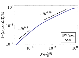
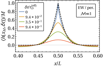
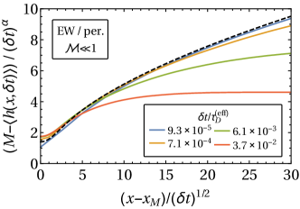
Figure 4: Averaged profile $\langle h(x,\delta t)\rangle$ obtained for the EW equation [Eq. 1] with periodic boundary conditions in the transient regime ($\mathcal{M}\ll 1$). The first passage of the height $M$ occurs at the time $\delta t=0$. Utilizing translational invariance, the individual profiles obtained from simulation are shifted such that the height $M$ is reached at location $x_{M}=L/2$. Time is normalized to the diffusion time scale $\tau_{D}$ [Eq. 17] using for the exponent $z$ an effective value of $1/(2\alpha)\simeq 1.7$ ($\alpha\simeq 0.29)$ instead of $2$, as implied by panel (a). (a) Time-evolution of the peak of the profile, $\langle h(x_{M},\delta t)\rangle$, which exhibits an intermediate asymptotic regime $M-\langle h(x_{M},\delta t)\rangle\propto\delta t^{\alpha}$ with $\alpha\simeq 0.29$. (b) Spatio-temporal evolution of the averaged profile. The solid curves represent the profiles obtained from numerical simulations, while the dashed curve indicates the asymptotic profile predicted by WNT in Eq. 28, taking $T$ as a fit parameter. (c) Test of the dynamic scaling behavior of $\langle h(x,\delta t)\rangle$ as predicted by WNT according to Eq. 30, using a value of $1/z\simeq 0.28$. The dashed curve represents the scaling function $c\tilde{\mathcal{H}}$ in Eq. 31, with a prefactor $c\simeq 1.4$ determined from a fit.

We now turn to the first-passage dynamics of a profile governed by Eq. 1 with periodic and Dirichlet boundary conditions.

IV.1 Summary of WNT

Before discussing the simulation results, we summarize a few relevant predictions of WNT of the EW equation (see Ref. Gross (2017) for details). The following expressions for $h(x,\delta t)$ are to be understood as the leading-order contribution to the averaged profile $\langle h(x,\delta t)\rangle$. Note that, differently from Ref. Gross (2017), we use $\delta t=T-t$ as the time variable. Within WNT, the first-passage time $T$ is a fixed parameter and the transient and the equilibrium regime are distinguished by the value of $T/\tau$. In the transient regime ($T\ll\tau$), a scaling profile at time $\delta t=0$ results from WNT as

$$h(x,\delta t=0)\big{|}_{T\ll\tau}=M\mathcal{H}\left(\frac{x-L/2}{(2T)^{1/z}}\right),\qquad z=2,$$ (28)

with the scaling function

$$\mathcal{H}(\xi)=\exp\left(-\frac{\xi^{2}}{4}\right)+\frac{1}{2}\sqrt{\pi}|\xi|\left[\mathrm{erf}\left(\frac{|\xi|}{2}\right)-1\right].$$ (29)

For $0<\delta t\ll T$, one obtains the dynamic scaling profile

$$h(x,\delta t)\Big{|}_{\begin{subarray}{c}T\ll\tau\\ \delta t\ll T\end{subarray}}=M-M\left(\frac{\delta t}{2T}\right)^{1/z}\tilde{\mathcal{H}}\left(\frac{x-L/2}{\delta t^{1/z}}\right),\qquad z=2,$$ (30)

with the scaling function

$$\tilde{\mathcal{H}}(\xi)=\exp\left(-\frac{\xi^{2}}{4}\right)+\frac{1}{2}\sqrt{\pi}\,\xi\,\mathrm{erf}\left(\frac{\xi}{2}\right).$$ (31)

When applying Eqs. 28 and 30 to simulation results, we consider the quantity $T$ as a fit parameter. In the equilibrium regime ($T\gg\tau$) for $\delta t=0$, one finds the following asymptotic first-passage profiles for periodic and Dirichlet boundary conditions, respectively:

$$h^{\text{(p)}}(x,\delta t=0)\big{|}_{T\to\infty}/M =1-6\Bigg{|}\frac{x}{L}-\frac{1}{2}\Bigg{|}+6\left(\frac{x}{L}-\frac{1}{2}\right)^{2},$$ (32a)

$$h^{\text{(D)}}(x,\delta t=0)\big{|}_{T\to\infty}/M =1-\left|1-\frac{2x}{L}\right|.$$ (32b)

These profiles attain their maximum at $x_{M}=L/2$. They follow readily from the constrained minimization of the corresponding equilibrium free energy. For times $0<\delta t\ll T$, one finds a dynamic scaling form,

$$h(x,\delta t)\big{|}_{T\gg\tau}\simeq M-M(\delta t)^{1/z}\Gamma(1-1/z)\tilde{\mathcal{H}}\left(\frac{x-L/2}{\delta t^{1/z}}\right),\qquad z=2,$$ (33)

with the same scaling function as in Eq. 31. Note that, unless otherwise indicated, the above scaling forms apply to all boundary conditions considered here. Exact analytical expressions for the profile $h(x,t)$ obtained within WNT can be found in Ref. Gross (2017) and are not repeated here.

We emphasize that the above expressions pertain to a continuum system. As shown in Ref. Gross (2017), the presence of a microscopic cutoff (e.g., a lattice constant) modifies the dynamics for times $\delta t\lesssim\tau_{\times}$, where $\tau_{\times}$ is the crossover time in Eq. 15. Upon taking this effect into account, the time-evolution of the profile $h(x,\delta t)$ at $x=x_{M}$ is given within WNT by

$$1-h(x_{M},\delta t)/M\propto\begin{cases}\delta t,\qquad&\delta t\lesssim\tau_{\times},\\ \delta t^{1/z},\qquad&\delta t\gtrsim\tau_{\times}.\end{cases}$$ (34)

This result is independent of the boundary conditions and applies to both the transient and equilibrium regime [see Eqs. 30 and 33].

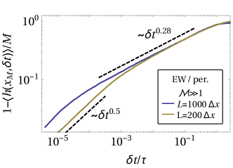
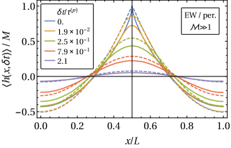
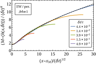
Figure 5: Averaged profile $\langle h(x,\delta t)\rangle$ obtained for the EW equation [Eq. 1] with periodic boundary conditions in the equilibrium regime ($\mathcal{M}\gg 1$). The first passage of the height $M$ occurs at the time $\delta t=0$. Utilizing translational invariance, the individual profiles obtained from simulation are shifted such that the height $M$ is reached at location $x_{M}=L/2$. Time is normalized to the relaxation time scale $\tau$ [see Eq. 14]. (a) Time-evolution of the peak of the profile, $\langle h(x_{M},\delta t)\rangle$, for two different system sizes (in units of the lattice spacing $\Delta x$). In the intermediate asymptotic regime one has $M-\langle h(x_{M},\delta t)\rangle\propto\delta t^{\alpha}$ with $\alpha\simeq 0.28$. (b) Spatio-temporal evolution of the averaged profile. The solid curves represent the profiles obtained from numerical simulations with $L=400\Delta x$, $\mathcal{M}\simeq 1.6$, while the dashed curves indicate the prediction of WNT [see Eq. (2.19) in Ref. Gross (2017) ]. (c) Test of the dynamic scaling behavior of $\langle h(x,\delta t)\rangle$ as predicted by WNT according to Eq. 33, using a value of $1/z\simeq 0.3$. The dashed curve represents the scaling function $c\tilde{\mathcal{H}}$ in Eq. 31, with a prefactor $c\simeq 1.6$ determined from a fit.

IV.2 Periodic boundary conditions

We now turn to the discussion of the first-passage properties of a profile governed by the EW equation [Eq. 1] with periodic boundary conditions. We recall that, in this case, the constraint of zero mass [Eq. 9] is imposed via Eq. 10 at each time step in the simulation. (Within WNT, this constraint is reflected by the absence of the zero mode in the series solution for the profile, see Ref. Gross (2017).) Figure 3 illustrates the spatial shape of the averaged profile at the first-passage event, $\langle h(x,\delta t=0)\rangle$, for various reduced heights $\mathcal{M}$ . The asymptotic scaling profiles predicted by WNT in the transient and the equilibrium regime [Eqs. 32a and 28, solid lines] agree well with the numerical results in the limits $\mathcal{M}\ll 1$ and $\mathcal{M}\gg 1$. According to Eq. 28, the analytical profile in the transient regime still depends on $T$, which is considered here as a fit parameter and effectively controls the width of the profile. Furthermore, since Eq. 28 is obtained by neglecting the mass constraint [Eq. 9], it applies only to an inner region of the profile. In contrast, the full solution of WNT provides an accurate description for $\mathcal{M}\lesssim 1$ also in the outer regions, as is illustrated below. Part of the remaining discrepancies between the analytically and numerically obtained profiles in Fig. 3 can be attributed to the fact that WNT neglects fluctuations around the saddle point solution. Such fluctuations can give rise to an effective repulsion from the boundary. We will return to this aspect in Section VI.

In Figs. 4 and 5, the spatio-temporal evolution of the averaged profile approaching the first-passage event $\langle h(x=x_{M},0)\rangle=M$ is illustrated in the transient and equilibrium regimes, respectively. As observed in Fig. 4(a) and 5(a) , both in the transient and the equilibrium regime, the peak of the profile, $\langle h(x_{M},\delta t)\rangle$ (with $x_{M}=L/2$), approaches the maximum height $M$ algebraically,

$$M-\langle h(x_{M},\delta t)\rangle\propto\delta t^{\alpha}.$$ (35)

For times $\delta t$ larger than a cross-over time $\tau_{\times}$ (see below), one obtains an exponent

$$\alpha\simeq 0.28-0.3,$$ (36)

while $\alpha=\alpha_{0}\simeq 0.5$ for $\delta t\lesssim\tau_{\times}$. The extent of the intermediate asymptotic regime described by Eq. 36 grows upon increasing the system size $L$, as illustrated in Fig. 5. Notably, the above values of the exponent $\alpha$ differ significantly from the values $\alpha_{\text{WNT}}=1/z=1/2$ and $\alpha_{\text{0,WNT}}=1$ predicted by WNT in Eq. 34. An explanation of these findings, which are analogously obtained also for the other models considered in this study, is provided in Section VI. As seen in Fig. 5, in the equilibrium regime, the first-passage evolution of the profile happens essentially within a timescale of the order of $\tau^{\text{(p)}}$ [see Eq. 14], as predicted by WNT. In the transient regime, the characteristic time scale is taken here to be the effective diffusion time $\tau_{D}^{\text{eff}}$. The latter is defined by Eq. 17, using for the dynamic exponent $z$ the effective value $1/(2\alpha)\simeq 1.7$ with $\alpha$ given in Eq. 36. Using instead the value $z=2$ predicted by WNT leads to a significant underestimation of the first-passage time scale. The non-vanishing cross-over time $\tau_{\times}$ arises due to the finite lattice spacing $\Delta x$ in the simulations. In agreement with the numerical data, Eq. 15 predicts $\tau_{\times}/\tau^{\text{(p)}}\sim 10^{-5}$ ($L=1000\Delta x$) and $\tau_{\times}/\tau^{\text{(p)}}\sim 2\times 10^{-4}$ ($L=200\Delta x$) for the two system sizes considered in Fig. 5.

In Figs. 4(b) and 5(b), the shape of the averaged profile is illustrated for various times $\delta t$ (solid lines). In Fig. 5(b) the dashed lines represent the time-dependent profiles obtained within WNT [Eq. I-(2.19)]. Since the actual time-dependence of $\langle h(x,t)\rangle$ differs from the prediction of WNT due to a different value of the dynamic exponent $\alpha$, analytical profiles do in general not match the numerical solutions well for $\delta t>0$. These discrepancies are found to be more severe in the transient regime [Fig. 4(b)], where we show only the scaling profile given in Eq. 28 (dashed line).

In Figs. 4(c) and 5(c), the dynamic scaling behavior asymptotically predicted by WNT [see Eqs. 33 and 30] is tested. To this end, the profile height $\langle h\rangle$ and the coordinate $x$ are rescaled accordingly and the scaling function $c\tilde{H}$ in Eq. 31 is fitted via the parameter $c$. In order to account for the renormalization of the dynamic exponent $\alpha$, we use for $1/z$ in Eqs. 33 and 30 an effective value which is close to the value for $\alpha$ reported in Eq. 36 . As shown in Figs. 4(c) and 5(c), this results in a satisfactory matching (in an inner region) of the numerical profiles with the scaling function $\tilde{H}$ in Eq. 31 (dashed line). The outer parts of the profiles deviate from the scaling function due to the influence of the boundary conditions.

IV.3 Dirichlet boundary conditions

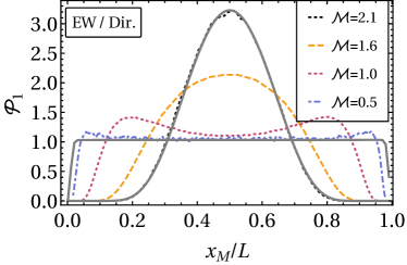
Figure 6: Distribution $\mathcal{P}_{1}(x_{M})$ of the spatial location $x_{M}$ at which the profile passes the height $M$ for the first time in the case of the EW equation [Eq. 1] with Dirichlet boundary conditions. The broken lines represent simulation data for various reduced heights $\mathcal{M}$. The solid curve with the flat center represents the prediction of WNT asymptotically in the transient regime ($\mathcal{M}\to 0$, see Ref. Gross (2017)). The bell-shaped solid curve pertains to the equilibrium regime ($\mathcal{M}\gtrsim 1$) and is given by Eq. I-(2.16), evaluated using $\eta M^{2}/DL\simeq 1.8$ and $T/\tau^{\text{(D)}}\gg 1$, as determined from a fit.

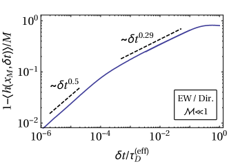
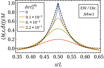
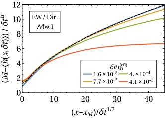
Figure 7: Averaged profile $\langle h(x,\delta t)\rangle$ obtained for the EW equation [Eq. 1] with Dirichlet boundary conditions in the transient regime ($\mathcal{M}\ll 1$). The first passage of the height $M$ occurs at the time $\delta t=0$. Time is normalized to the diffusion time scale $\tau_{D}$ [Eq. 17] using for the exponent $z$ an effective value of $1/(2\alpha)\simeq 1.7$ ($\alpha\simeq 0.29)$ instead of $2$, as implied by panel (a). (a) Time-evolution of the peak of the profile, $\langle h(x_{M},\delta t)\rangle$, which exhibits an intermediate asymptotic regime $M-\langle h\rangle\propto\delta t^{\alpha}$ with $\alpha\simeq 0.29$. (b) Spatio-temporal evolution of the averaged profile. The solid curves represent the profiles obtained from numerical simulations, while the dashed curve indicates the asymptotic profile predicted by WNT in Eq. 28, taking $T$ as a fit parameter. (c) Test of the dynamic scaling behavior of $\langle h(x,t)\rangle$ as predicted by WNT in Eq. 30, using a value of $1/z\simeq 0.29$. The dashed curve represents the scaling function $c\tilde{\mathcal{H}}$ in Eq. 31, with a prefactor $c\simeq 1.3$ determined from a fit. In order to account for the localized nature of the profiles in the transient regime, in all panels the individual profiles are shifted before averaging such that $h^{(s)}(L/2,T^{(s)})=M$ [see Eq. 24].

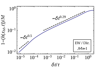
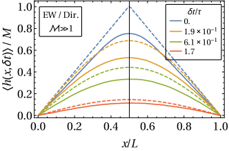
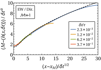
Figure 8: Averaged profile $\langle h(x,\delta t)\rangle$ for the EW equation [Eq. 1] with Dirichlet boundary conditions in the equilibrium regime ($\mathcal{M}\gg 1$). The first passage of the height $M$ occurs at the time $\delta t=0$. Time is normalized to the relaxation time $\tau^{\text{(D)}}$ [see Eq. 14]. (a) Time-evolution of the peak of the profile, $\langle h(x_{M},\delta t)\rangle$, which exhibits an intermediate asymptotic regime $M-\langle h\rangle\propto\delta t^{\alpha}$ with $\alpha\simeq 0.29$. (b) Spatio-temporal evolution of the averaged profile. The solid curves represent the profiles obtained from numerical simulations, while the dashed curves indicate the prediction of WNT [see Eq. I-(2.21)]. (c) Test of the dynamic scaling behavior of $\langle h(x,t)\rangle$ as predicted by WNT in Eq. 33, using a value of $1/z\simeq 0.29$. The dashed curve represents the scaling function $c\tilde{\mathcal{H}}$ in Eq. 31, with a prefactor $c\simeq 1.5$ determined from a fit. In order to properly exhibit the scaling behavior, in panels (a) and (c) the individual profiles are shifted before averaging such that $h^{(s)}(L/2,T^{(s)})=M$ [see Eq. 24].

We now turn to the rare event dynamics of a profile governed by the EW equation with standard Dirichlet boundary conditions [Eq. 6]. We recall that, in this case, the mass constraint in Eq. 9 is not fulfilled by the individual realizations of the profile. The probability distribution $\mathcal{P}_{1}(x_{M})$ of the location $x_{M}$ of the first-passage event [see Eq. 11] is shown in Fig. 6 for various reduced heights $\mathcal{M}$. For $\mathcal{M}\ll 1$, $\mathcal{P}_{1}$ is essentially flat, in agreement with the prediction of WNT in the transient regime (see Ref. Gross (2017)). For $\mathcal{M}\gg 1$, instead, the first-passage event is most likely to occur at the center of the system. In this regime, $\mathcal{P}_{1}$ can be well fitted by the analytical expression reported in Eq. I-(2.16), using a value of $\eta M^{2}/DL\simeq 1.8$ and $T/\tau^{\text{(D)}}\gg 1$ (the precise value of the latter parameter is immaterial since $\mathcal{P}_{1}$ becomes independent of it provided it is sufficiently large). In the crossover region between the transient and the equilibrium regime, $\mathcal{P}_{1}$ depends within WNT on both $T/\tau^{\text{(D)}}$ and $\eta M^{2}/DL$ and, therefore, a fit is less meaningful. Differently from WNT, $\mathcal{P}_{1}$ develops two maxima near the boundaries for $\mathcal{M}\sim\mathcal{O}(1)$.

In Figs. 7 and 8, the spatio-temporal evolution of the averaged profile in the transient and equilibrium regimes, respectively, is illustrated. Since the distribution $\mathcal{P}_{1}(x_{M})$ of the first-passage location is flat in the transient regime, the averaged profiles shown in Fig. 7 are obtained by shifting each realization such that the first-passage event occurs at $x_{M}=L/2$ [see Eq. 24]. Since the profile is strongly localized in the transient regime, such a shift does not significantly affect its averaged shape. As shown in Fig. 7(b), a fit via the parameter $T$ of the asymptotic profile of WNT reported in Eq. 28 yields satisfactory agreement with the data. In the equilibrium regime, the averaged profile is computed according to Eq. 24 without a shift ($X^{(s)}=0$). In this case, the finite width of $\mathcal{P}_{1}(x_{M})$ [see Fig. 6] is reflected by the rather strong deviation of $\langle h(x,\delta t)\rangle$ from the prediction of WNT [Eq. 32b, dashed lines in Fig. 8(b)] as well as by the fact that $\langle h(x_{M},\delta t=0)\rangle<M$. These deviations diminish upon increasing $\mathcal{M}$.

As shown in Figs. 7 and 8, both in the transient and equilibrium regime, the peak $\langle h(x_{M},\delta t)\rangle$ follows the same algebraic time-evolution as in Eq. 35 and is characterized by two distinct dynamic exponents. Similarly to periodic boundary conditions [see Eq. 36], we obtain $\alpha\simeq 0.29$ and $\alpha=\alpha_{0}\simeq 0.5$ for the values of the dynamic exponent at late and early times $\delta t$, respectively, which are different from the prediction of WNT in Eq. 34. Despite this discrepancy, the time-dependent averaged profiles of WNT qualitatively match the simulation results in the equilibrium regime [see Fig. 8(b)]. Deviations are more significant in the transient regime (not shown), although the qualitative behavior agrees with WNT.

In Fig. 7(c) and 8(c), the dynamic scaling behavior predicted in Eqs. 33 and 30, respectively, is tested. Using an effective value of $1/z=\alpha\simeq 0.29$ for the dynamic exponent, a satisfactory fit of the numerical profiles with the scaling function in Eq. 31 is obtained. The agreement between WNT and simulations generally improves as $\delta t\to 0$.

V Mullins-Herring equation

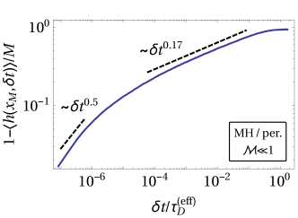
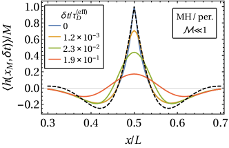
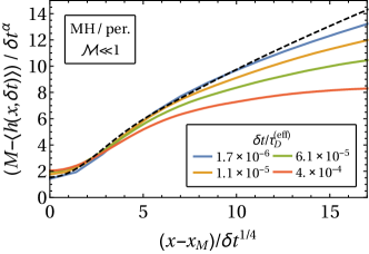
Figure 9: Averaged profile $\langle h(x,\delta t)\rangle$ for the MH equation [Eq. 2] with periodic boundary conditions in the transient regime ($\mathcal{M}\ll 1$). The first passage of the height $M$ occurs at the time $\delta t=0$. Utilizing translational invariance, the individual profiles obtained from simulation are shifted such that the height $M$ is reached at location $x_{M}=L/2$. Time is normalized to the diffusion time scale $\tau_{D}$ [Eq. 17] using for the exponent $z$ an effective value of $1/(2\alpha)\simeq 2.9$ ($\alpha\simeq 0.17)$ instead of $4$, as implied by panel (a). (a) Time-evolution of the peak of the profile, $\langle h(x_{M},\delta t)\rangle$, which exhibits an intermediate asymptotic regime, $M-\langle h(x_{M},\delta t)\rangle\propto\delta t^{\alpha}$ with $\alpha\simeq 0.17$. (b) Spatio-temporal evolution of the averaged profile. The solid curves represent numerical simulations, while the dashed curve indicates the asymptotic profile predicted by WNT in Eq. 37, taking $T$ as a fit parameter. (c) Test of the dynamic scaling behavior of $\langle h(x,\delta t)\rangle$ as predicted by WNT in Eq. 39, using a value of $1/z\simeq 0.19$. The dashed curve represents the scaling function $c\tilde{\mathcal{H}}$ in Eq. 40, with a prefactor $c\simeq 1.4$ determined from a fit. In order to account for the localized nature of the profile in the transient regime, in all panels the individual profiles are shifted before averaging such that $h^{(s)}(L/2,T^{(s)})=M$ [see Eq. 24].

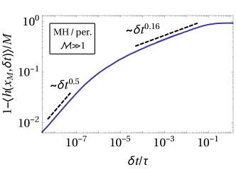
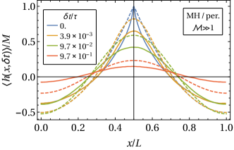
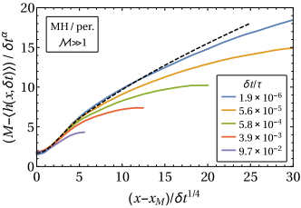
Figure 10: Averaged profile $\langle h(x,\delta t)\rangle$ for the MH equation [Eq. 2] with periodic boundary conditions in the equilibrium regime ($\mathcal{M}\gg 1$). The first passage of the height $M$ occurs at the time $\delta t=0$. Utilizing translational invariance, the individual profiles obtained from simulation are shifted such that the height $M$ is reached at location $x_{M}=L/2$. Time is normalized to the relaxation time $\tau^{\text{(p)}}$ [Eq. 14]. (a) Time-evolution of the peak of the profile, $\langle h(x_{M},\delta t)\rangle$, which exhibits an intermediate asymptotic regime $M-\langle h(x_{M},\delta t)\rangle\propto\delta t^{\alpha}$ with $\alpha\simeq 0.16$. (b) Spatio-temporal evolution of the averaged profile. The solid curves represent the numerical simulations, while the dashed curves indicate the prediction of WNT [see Eq. I-(3.17) as well as Ref. Meerson and Vilenkin (2016)]. (c) Test of the dynamic scaling behavior of $\langle h(x,t)\rangle$ as predicted by WNT according to Eq. 44, using a value of $1/z\simeq 0.17$. The dashed curve represents the scaling function $c\tilde{\mathcal{H}}$ in Eq. 40, with a prefactor $c\simeq 1.7$ determined from a fit.

We proceed with the discussion of the first-passage dynamics for the MH equation [Eq. 2]. For the considered boundary conditions, the mass [Eq. 8] is conserved in time and, in fact, $\mathcal{A}([h],t)=0$ owing to the initial condition in Eq. 4. Due to the larger value $z=4$ of the dynamic index [see Eq. 14], simulations are more time-demanding than for the EW equation. Moreover, it turns out that the cross-over regions between the different asymptotic regimes are broader, making it more difficult to identify clear power-laws.

V.1 Summary of WNT

Before proceeding to the simulation results, we summarize the essential predictions of WNT (see Ref. Gross (2017), as well as Ref. Meerson and Vilenkin (2016) in the case of periodic boundary conditions). As before, we use $\delta t=T-t$ as the time variable and the following expressions for $h$ are to be understood as the leading-order contributions to the averaged profile $\langle h\rangle$. Asymptotically for $T\to 0$ in the transient regime, one obtains the following static scaling profile at the first-passage event:

$$h(x,\delta t=0)\big{|}_{T\ll\tau}=M\mathcal{H}\left(\frac{x-L/2}{(2T)^{1/z}}\right),\qquad z=4,$$ (37)

with the scaling function

$$\mathcal{H}(\xi)={}_{1}F_{3}\left(-\frac{1}{4};\frac{1}{4},\frac{1}{2},\frac{3}{4};\frac{\xi^{4}}{256}\right)+\xi^{2}\frac{\Gamma\left(\frac{1}{4}\right)}{8\Gamma\left(\frac{3}{4}\right)}{}_{1}F_{3}\left(\frac{1}{4};\frac{3}{4},\frac{5}{4},\frac{3}{2};\frac{\xi^{4}}{256}\right)-\frac{\pi}{2\Gamma\left(\frac{3}{4}\right)}|\xi|,$$ (38)

which applies to periodic as well as Dirichlet no-flux boundary conditions. ${}_{1}F_{3}$ is a hypergeometric function Olver et al. (2010). A dynamic scaling profile for times $\delta t>0$ with $\delta t\ll T$ is given, to leading order in $\delta t/T$, by

$$h(x,\delta t)\big{|}_{\begin{subarray}{c}T\ll\tau\\ \delta t\ll T\end{subarray}}=M-M\left(\frac{\delta t}{2T}\right)^{1/z}\tilde{\mathcal{H}}\left(\frac{x-L/2}{(\delta t)^{1/z}}\right),\qquad z=4,$$ (39)

with the scaling function

$$\tilde{\mathcal{H}}(\xi)={}_{1}F_{3}\left(-\frac{1}{4};\frac{1}{4},\frac{1}{2},\frac{3}{4};\frac{\xi^{4}}{256}\right)+\xi^{2}\frac{\Gamma\left(\frac{1}{4}\right)}{8\Gamma\left(\frac{3}{4}\right)}{}_{1}F_{3}\left(\frac{1}{4};\frac{3}{4},\frac{5}{4},\frac{3}{2};\frac{\xi^{4}}{256}\right).$$ (40)

In the equilibrium regime, the static profile $h^{\text{(p)}}(x,\delta t=0)|_{T\to\infty}$ minimizing the corresponding free energy for periodic boundary conditions (see Ref. Gross (2017)) coincides with the one in Eq. 32a. For Dirichlet no-flux boundary conditions, instead, one finds

$$h^{(\mathrm{D}^{\prime})}(x,\delta t=0)\big{|}_{T\to\infty}=h^{\text{(p)}}(x+L/2-x_{M},\delta t=0)\big{|}_{T\to\infty}$$ (41)

with

$$x_{M}^{(\mathrm{D}^{\prime})}\big{|}_{T\to\infty}=\frac{L}{2}\left(1\pm\frac{1}{\sqrt{3}}\right).$$ (42)

For definiteness, we choose henceforth the smaller value for $x_{M}^{(\mathrm{D}^{\prime})}$, such that Eq. 41 can be explicitly written as

$$h^{(\mathrm{D}^{\prime})}(x,\delta t=0)\big{|}_{T\to\infty}/M=\begin{cases}\displaystyle 6\frac{x}{L}\left(\frac{x}{L}+\frac{1}{\sqrt{3}}\right),\qquad&x\leq x_{M}^{(\mathrm{D}^{\prime})},\\ \displaystyle 6\left(\frac{x}{L}-1\right)\left(\frac{x}{L}-1+\frac{1}{\sqrt{3}}\right),&x>x_{M}^{(\mathrm{D}^{\prime})}.\end{cases}$$ (43)

In the equilibrium regime for times $\delta t>0$ with $\delta t\ll T$, a dynamic scaling profile for periodic and Dirichlet boundary conditions is given by

$$h(x,\delta t)\big{|}_{T\gg\tau}\simeq M-M(\delta t)^{1/z}\Gamma(1-1/z)\tilde{\mathcal{H}}\left(\frac{x-x_{M}}{\delta t^{1/z}}\right),\qquad z=4,$$ (44)

with the same scaling function as in Eq. 40. Note that the above expressions pertain to a continuum system. In the presence of an upper bound to the eigenmode spectrum, the time evolution of the peak $h(x_{M},\delta t)$ of the profile exhibits two regimes:

$$1-h(x_{M},\delta t)/M\propto\begin{cases}\delta t,\qquad&\delta t\lesssim\tau_{\times},\\ \delta t^{1/z},\qquad&\delta t\gtrsim\tau_{\times},\end{cases}$$ (45)

where $\tau_{\times}$ is the crossover time [see Eq. 15]. As was the case for the EW equation [see Eq. 34], Eq. 45 is independent of the boundary conditions and applies to both the transient and the equilibrium regime. Explicit expressions for the first-passage profiles obtained within WNT for all times are reported in Ref. Gross (2017).

V.2 Periodic boundary conditions

Here, we discuss simulation results obtained for the MH equation with periodic boundary conditions. Figures 9 and 10 illustrate the time evolution of the averaged profile $\langle h(x,\delta t)\rangle$ towards the first-passage event in the transient and equilibrium regimes, respectively. As shown in panels (a), in both regimes, the peak $\langle h(x_{M}=L/2,\delta t)\rangle$ approaches the height $M$ via a power-law, $M-\langle h(x_{M}=L/2,\delta t)\rangle\propto\delta t^{\alpha}$, with $\alpha\simeq 0.16-0.17$ at intermediate times ($\delta t\gtrsim\tau_{\times}$) and $\alpha=\alpha_{0}\simeq 0.5$ at early times ($\delta t\lesssim\tau_{\times}$). Analogously to the finding for EW dynamics (see Section IV), these values of the dynamical exponent are significantly smaller than the prediction $\alpha=1/4$ and $\alpha_{0}=1$ obtained from WNT [Eq. 45]. This finding is rationalized in Section VI below. In order to account for this quantitative change in the dynamics, in Fig. 9 we rescale time by an effective diffusion time scale $\tau_{D}^{\text{eff}}$, which results from Eq. 17 by replacing $z$ by the value $1/(2\alpha)\simeq 2.9-3.1$ [cf. Section IV.2]. For the systems considered in Figs. 9 and 10, the crossover time defined in Eq. 15 follows as $\tau_{\times}/\tau^{\text{(p)}}\simeq 2\times 10^{-7}$ and $6\times 10^{-8}$, respectively, which is in good agreement with the simulation data.

Figs. 9(b) and 10(b) illustrate the spatio-temporal evolution of the averaged profile. The deviations from the prediction of WNT (dashed curves) can be mainly attributed to the fact that simulations operate in the finite-noise regime. As shown in 10(b), in the equilibrium regime, the time-dependent profile shapes obtained from simulations are qualitatively similar to WNT, although the difference in the value of the dynamic exponent $\alpha$ leads to a faster time evolution in the latter case.

Figs. 9(c) and 10(c) demonstrate that, in an inner region, the profiles follow the scaling behavior implied by Eqs. 39 and 44. The agreement improves upon decreasing $\delta t$. Scaling collapse is obtained here by using in Eqs. 39 and 44 for $1/z$ an effective value of $0.17-0.19$, consistent with the value of the exponent ($\alpha$) that governs the time-evolution of the peak of the profile [see Figs. 10 and 9].

V.3 Dirichlet no-flux boundary conditions

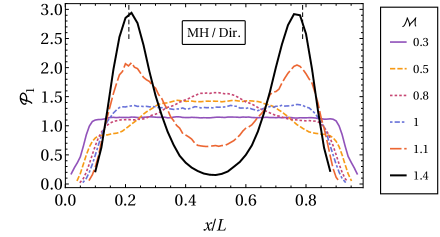
Figure 11: Probability distribution $\mathcal{P}_{1}(x_{M})$ obtained for the MH equation [Eq. 2] with Dirichlet no-flux boundary conditions and for various reduced heights $\mathcal{M}$ [Eq. 22]. $x_{M}$ denotes the spatial location at which the profile passes the height $M$ for the first time. Asymptotically for $\mathcal{M}\to 0$ in the transient regime, $\mathcal{P}_{1}$ is generally flat (except at the boundaries). For Dirichlet no-flux boundary conditions in the equilibrium regime ($\mathcal{M}\gtrsim 1$), two peaks emerge at the locations given in Eq. 42.

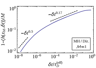
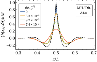
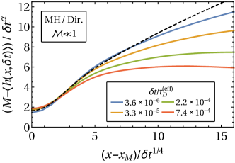
Figure 12: Averaged profile $\langle h(x,\delta t)\rangle$ for the MH equation [Eq. 2] with Dirichlet no-flux boundary conditions in the transient regime ($\mathcal{M}\ll 1$). The first passage of the height $M$ occurs at the time $\delta t=0$. Time is normalized to the diffusion time scale $\tau_{D}$ [Eq. 17] using for the exponent $z$ an effective value of $1/(2\alpha)\simeq 2.9$ ($\alpha\simeq 0.17)$ instead of $4$, as suggested by panel (a). (a) Time-evolution of the peak of the profile, $\langle h(x_{M},\delta t)\rangle$, which exhibits an intermediate asymptotic regime $M-\langle h(x_{M},\delta t)\rangle\propto\delta t^{\alpha}$ with $\alpha\simeq 0.17$. (b) Spatio-temporal evolution of the averaged profile. The solid curves represent the numerical simulations, while the dashed curve indicates the asymptotic profile predicted by WNT in Eq. 37, taking $T$ as a fit parameter. (c) Test of the dynamic scaling behavior of $\langle h(x,\delta t)\rangle$ as predicted by WNT in Eq. 39, using an effective value of $1/z\simeq 0.17$. The dashed curve represents the scaling function $c\tilde{\mathcal{H}}$ in Eq. 40, with a prefactor $c\simeq 1.3$ determined from a fit. In order to account for the localized nature of the individual profiles, data in panels (a) and (c) are obtained by shifting the individual profiles before averaging such that $h^{(s)}(L/2,T^{(s)})=M$ [see Eq. 24].

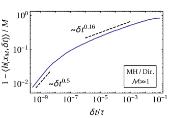
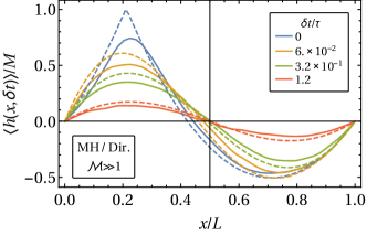
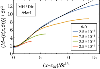
Figure 13: Averaged profile $\langle h(x,\delta t)\rangle$ for the MH equation [Eq. 2] with Dirichlet no-flux boundary conditions in the equilibrium regime ($\mathcal{M}\gg 1$). The first passage of the height $M$ occurs at the time $\delta t=0$. Time is normalized to the relaxation time $\tau^{(\mathrm{D}^{\prime})}$ [Eq. 14]. (a) Time-evolution of the peak of the profile, $\langle h(x_{M},\delta t)\rangle$, which exhibits an intermediate asymptotic regime $M-\langle h(x_{M},\delta t)\rangle\propto\delta t^{\alpha}$ with $\alpha\simeq 0.16$. (b) Spatio-temporal evolution of the averaged profile. The solid curves represent the numerical simulations, while the dashed curves indicate the prediction of WNT [see Eq. I-(3.19)]. (c) Test of the dynamic scaling behavior of $\langle h(x,\delta t)\rangle$ as predicted by WNT in Eq. 44, using a value of $1/z\simeq 0.17$. The dashed curve represents the scaling function $c\tilde{\mathcal{H}}$ in Eq. 40, with a prefactor $c\simeq 2$ determined from a fit.

In contrast to standard Dirichlet boundary conditions, which entail a fixed chemical potential at the boundaries (see Ref. Gross (2017)) and thus a non-conserved mass, the no-flux condition [Eq. 7] ensures mass conservation for the MH equation. In fact, due to the initial condition in Eq. 4, the mass $\mathcal{A}([h],t)$ [Eq. 8] vanishes at all times. Figure 11 shows the probability distribution $\mathcal{P}_{1}^{(\mathrm{D}^{\prime})}(x_{M})$ of the first-passage location $x_{M}$. We find that the essential predictions of WNT [see Fig. I-7] are recovered by the simulations. Asymptotically in the transient regime ($\mathcal{M}\to 0$), $\mathcal{P}_{1}$ is generally constant as a function of $x_{M}$ for $0<x_{M}<L$. At the boundaries, $\mathcal{P}_{1}^{(\mathrm{D}^{\prime})}$ vanishes as a consequence of Dirichlet boundary conditions. Upon increasing $\mathcal{M}$ towards values of $\mathcal{O}(1)$, a peak develops in the central region of $\mathcal{P}_{1}^{(\mathrm{D}^{\prime})}$. Upon increasing $\mathcal{M}$ further, this peak diminishes, while two symmetric peaks develop near the location $x_{M}^{(\mathrm{D}^{\prime})}$ [Eq. 42] predicted by WNT. One expects $\mathcal{P}_{1}^{(\mathrm{D}^{\prime})}(x_{M})\to\delta\left(x_{M}\pm x_{M}^{(\mathrm{D}^{\prime})}\right)$ as $\mathcal{M}\to\infty$, which represents a particular realization of the weak-noise limit.

In Figs. 12 and 13, the profile dynamics obtained from simulations in the transient and equilibrium regimes, respectively, is illustrated. In panels (a), the averaged time evolution of the peak, $\langle h(x_{M},\delta t)\rangle$, is shown as a function of the time $\delta t$ until the first-passage event. In order to account for the spread in the distribution of $x_{M}$, in these two panels $\langle h(x_{M},\delta t)\rangle$ is computed according to Eq. 24 by shifting the individual profiles $h^{(s)}$ to the common first-passage location $L/2$, such that $h^{(s)}(L/2,T^{(s)})=M$. The peak is found to evolve algebraically, $M-\langle h(x_{M},\delta t)\rangle\propto\delta t^{\alpha}$, with $\alpha=\alpha_{0}\simeq 0.5$ for times $\delta t\lesssim\tau_{\times}$ and $\alpha\simeq 0.16-0.17$ for $\tau_{\times}\lesssim\delta t\lesssim\tau^{(\mathrm{D}^{\prime})}$. These values for $\alpha$ practically coincide with the ones for periodic boundary conditions [Section V.2] and are further discussed in Section VI. In order to estimate the crossover time $\tau_{\times}$ [see Eq. 15], we assume that the largest mode which can be accommodated by the system is given by $k_{\times}\simeq 0.5L/\Delta x$ (see Section G.2 for further discussion). This renders the estimates $\tau_{\times}\simeq 2.4\times 10^{-7}\tau_{D}^{\text{eff}}$ and $\tau_{\times}\simeq 3.2\times 10^{-9}\tau^{(\mathrm{D}^{\prime})}$ in the transient and equilibrium regimes, respectively, which are seen to agree with the simulation data within an order of magnitude.

The time-dependent averaged profile $\langle h(x,\delta t)\rangle$ in the transient regime is illustrated in Fig. 12(b). The average [see Eq. 24] is computed here again by translating each profile $h^{(s)}$ to the common first-passage location $L/2$. This transformation does not significantly affect the profile shape because the profiles are strongly localized and the distribution $\mathcal{P}_{1}^{(\mathrm{D}^{\prime})}(x_{M})$ is approximately flat in the transient regime [see Fig. 11]. In the equilibrium regime, in contrast, $\mathcal{P}_{1}^{(\mathrm{D}^{\prime})}(x_{M})$ is symmetric around $L/2$ and the first-passage event is most likely to occur at either of the two locations given in Eq. 42. In this case, the averaged profile $\langle h(x,\delta t)\rangle$ shown in Fig. 13(b) is obtained by mirroring at $x=L/2$ all profiles $h^{(s)}$ which belong to a simulation with $x_{M}^{(s)}>L/2$. The spatio-temporal evolution of the profile displayed in the plots qualitatively agrees with the predictions of WNT (see Ref. Gross (2017)). As a consequence of the finite width of $\mathcal{P}_{1}^{(\mathrm{D}^{\prime})}$ around each of its two peaks, the maximum of $\langle h(x,\delta t)\rangle$ in Fig. 13(b) is smaller than $M$, despite the fact that each stochastic realization fulfills $h^{(s)}(x_{M}^{(s)},T^{(s)})=M$.

Close to the first-passage event, WNT predicts a universal dynamic scaling behavior of the profile, as expressed in Eqs. 39 and 44. As shown in Figs. 12(c) and 13(c), this property is recovered in the simulations: upon accounting for the renormalized dynamic exponent $1/z\to\alpha\simeq 0.17$, the profiles superimpose onto the scaling function $c\tilde{H}$ [Eq. 40] within an inner region, where $c$ is a fit parameter.

VI Discussion

As demonstrated in the preceding sections, a crucial difference between the results of the Langevin simulations and the predictions of WNT arises in the time-dependence of the averaged profile. Both in simulations and within WNT, the peak of the profile $\langle h(x_{M},\delta t)\rangle$ approaches the first-passage height $M$ algebraically,

$$M-\langle h(x_{M},\delta t)\rangle\propto\begin{cases}\delta t^{\alpha_{0}},\qquad\qquad&\delta t\lesssim\tau_{\times},\\ \delta t^{\alpha},\qquad&\tau_{\times}\lesssim\delta t\lesssim\tau.\end{cases}$$ (46)

However, simulations yield the values

$$\alpha_{0}\simeq 0.5,\qquad\alpha\simeq\begin{cases}0.27-0.3,\qquad&\text{EW},\\ 0.16-0.17,\qquad&\text{MH},\end{cases}$$ (47)

for the dynamic exponents, while WNT predicts (see Ref. Gross (2017))

$$\alpha_{\text{0,WNT}}=1,\qquad\alpha_{\text{WNT}}=1/z=\begin{cases}1/2,\qquad&\text{EW},\\ 1/4,\qquad&\text{MH}.\end{cases}$$ (48)

We emphasize that these results are independent of the boundary conditions and apply both in the transient and in the equilibrium regime. The crossover time $\tau_{\times}$ [Eq. 15] and the roughening time $\tau$ [Eq. 14] correspond to the relaxation time of the shortest and largest fluctuation wavelengths, respectively, that can be accommodated by the system. Since $\tau\propto L^{z}$, the intermediate asymptotic regime characterized by the exponent $\alpha$ dominates for sufficiently large systems. As detailed in the preceding sections, we furthermore recall that the time-evolution of the peak $\langle h(x_{M},\delta t)\rangle$ is determined based on a slightly different averaging procedure than the one used for the full profile [see also Eq. 24].

In order to gain a basic understanding of the discrepancy between Eq. 47 and (48), we first consider a (Markovian) Brownian walker $h(t)$, initially at $h(t=0)=0$, in the presence of an absorbing boundary at a fixed height $h=M$ (see Appendices D and C for details). Within WNT, the averaged path of the walker between the points $(t=0,h=0)$ and $(T,M)$, with $T$ fixed, is the one minimizing the associated action (see Appendix D). This results in a linear time-dependence of the walker approaching the absorbing boundary [see Eq. 101],

$$M-\langle h(\delta t)\rangle_{\text{WNT}}\propto\delta t.\qquad\text{(standard Brownian motion)}$$ (49)

As before, the average is defined here such that the first-passage event occurs at $\delta t=0$. For a Markovian Brownian walker, the averaged path to an impenetrable boundary can however also be calculated exactly, i.e., including all corrections beyond WNT (see Section C.1). For a fixed endpoint $(T,M)$, this yields

$$M-\langle h(\delta t)\rangle\propto\delta t^{1/2}\qquad\text{(standard Brownian motion, fixed $T$)}$$ (50)

as $\delta t\to 0$. The difference between the dynamic exponents in Eqs. 49 and 50 arises from the “entropic repulsion” (cf., e.g., Refs. Fisher (1984); Redner (2001)) exerted by the absorbing boundary onto fluctuations of the walker around the most-likely path described by WNT. Averaging also over the first-passage time distribution results in [see Section C.2]

$$M-\langle h(\delta t)\rangle\propto\delta t^{1/2}\qquad\text{(standard Brownian motion, first-passage path)}$$ (51)

and accordingly does not alter the trajectory asymptotically close to the boundary compared to Eq. 50. Far from the boundary, however, significant changes in the walker path are induced by this additional average (see Figs. 18 and 16).

The preceding results can be extended to fractional Brownian motion, i.e., to a Gaussian random process $h(t)$ characterized by the correlation function in Eq. 85. On its most-likely path, the walker approaches the endpoint $(t=T,h=M)$ algebraically [see Eq. 100]:

$$M-\langle h(\delta t)\rangle_{\text{WNT}}\propto\delta t^{2H},\qquad\text{(fractional Brownian motion)}$$ (52)

where $H$ is the Hurst exponent of the process ($H=1/2$ for standard Brownian motion). Beyond the weak-noise approximation, numerical simulations [see Section C.2.2] show that the actual first-passage path of a fractional Brownian walker behaves as

$$M-\langle h(\delta t)\rangle\propto\delta t^{H}.\qquad\text{(fractional Brownian motion)}$$ (53)

Note that, as in Eq. 51, the average is performed here also over the first-passage time distribution. Equations 52 and 53 are straightforward generalizations of the Markovian expressions in Eqs. 49 and 51. We conclude that taking into account fluctuation-induced interactions with the absorbing boundary effectively leads to a reduction of the dynamic exponent characterizing the averaged path of a Brownian walker from the value $2H$ predicted by WNT to the value $H$ .

We now apply these insights to a fluctuating profile $h(x,t)$. To this end, we recall that a tagged monomer $h(x_{M},t)$ follows a Gaussian stochastic process characterized by the Hurst exponents

$$H_{0}=1/2\qquad\text{and}\qquad H=\frac{1}{2z},\qquad\text{(profile)}$$ (54)

which, inter alia, determine the variance as [see Eq. 18]

$$\langle[\delta h(x_{M},t)]^{2}\rangle^{1/2}\sim\begin{cases}t^{H_{0}},\qquad&t\lesssim\tau_{\times}\\ t^{H},\qquad&\tau_{\times}\lesssim t\lesssim\tau.\end{cases}$$ (55)

For times $t\gtrsim\tau$, a tagged monomer experiences the “self-generated” effective potential of the mass-conserving profile, as reflected by the Gaussian equilibrium variance [see Eqs. 21 and 20].

We first turn to equilibrium initial conditions, for which the stochastic process described by Eqs. 55 and 54 is actually a fractional Brownian motion [see Eq. 18b]. In this case, Eq. 52 predicts, based on Eq. 54, the values $\alpha_{\text{0,WNT}}=2H_{0}=1$ and $\alpha_{\text{WNT}}=2H=1/z$ for the dynamic exponents in Eq. 46, in agreement with the explicit WNT results in Eq. 48. (Note that the weak-noise approximation here is insensitive to the presence of an impenetrable boundary.) Beyond WNT, Eq. 53 accordingly predicts

$$\alpha_{0}=H_{0}=\frac{1}{2},\qquad\alpha=H=\frac{1}{2z}=\begin{cases}1/4,\qquad\text{EW},\\ 1/8,\qquad\text{MH}\end{cases}\qquad\text{(prediction)}$$ (56)

for the dynamic exponents of a profile near a first-passage event. These values are indeed close to the simulation results in Eq. 47, especially in the case of the short-time exponent $\alpha_{0}$. Possible reasons for the discrepancy of the late-time exponent $\alpha$ are discussed below.

For non-equilibrium initial conditions, corresponding to the transient first-passage regime ($\mathcal{M}\ll 1$), the stochastic process underlying Eq. 55 is not a fractional Brownian motion [see Eq. 18a]. However, the above reasoning concerning the averaged profile essentially relies only on the Hurst characterization of the dynamics of a tagged monomer. In particular, this process has the same subdiffusive scaling behavior in the equilibrium and the transient regime, suggesting Eq. 56 to apply also in the latter. Indeed, the values for $\alpha$ obtained from the simulations in the two regimes are practically identical.

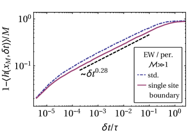
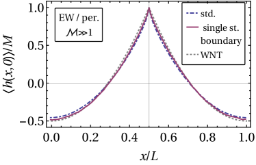
Figure 14: Effect of the spatial extension of the absorbing boundary condition on the first-passage behavior of a profile governed by the EW equation with periodic boundary conditions. Panel (a) shows the averaged time evolution of the peak $\langle h(x_{M},\delta t)\rangle$, while (b) shows the averaged profile at the first-passage event. The dash-dotted curves are obtained for an absorbing boundary acting on the whole profile [Eq. 11], which is the standard case in the present study. The solid curves, instead, correspond to an absorbing boundary acting only on the monomer at $x_{M}$ (“single site boundary”). The dotted curve in (b) represents the prediction of WNT [Eq. 32a].

The prediction in Eq. 56 is based on the equivalence of a fractional Brownian walker and a tagged monomer of an unconstrained interface. However, for the first-passage dynamics considered here, the absorbing boundary condition at the height $M$ [Eq. 11] is essential. This boundary condition constrains the profile as a whole and, owing to the long-range correlations of the profile, it can in principle lead to deviations in the behavior of a tagged monomer from the behavior expected for a single fractional Brownian walker. To which extent this effect is responsible for the discrepancy between the values for $\alpha$ reported in Eq. 47 and the predictions in Eq. 56 demands further studies.

Here it is possible to clarify at least the impact of the spatially extended nature of the absorbing boundary condition. To this end, we perform simulations in which an absorbing boundary acts only on a monomer at a single location $x_{M}$. Figure 14(a) shows $\langle h(x_{M},\delta t)\rangle$ as a function of time obtained in this case for the EW equation with periodic boundary conditions (solid curve). One observes that $\langle h(x_{M},\delta t)\rangle$ still follows the algebraic behavior in Eq. 46, with a value of $\alpha$ that is essentially identical to the one obtained for an absorbing boundary acting on all monomers [dash-dotted curve; see also Fig. 5]. As Fig. 14(b) shows, also the averaged profile at the first-passage event is not significantly affected by the spatially extended character of the absorbing boundary condition. This insensitivity can be attributed to the rather sharply peaked shape of the first-passage profile, which is already predicted by WNT [cf. Fig. 5(b)]. Overall, the results in Fig. 14 suggest that the spatial extension of the absorbing boundary has a negligible influence on the behavior of the averaged profile.

We finally remark that, in principle, also insufficiently large values of the system size $L$ or of the reduced height $\mathcal{M}$ can contribute to the deviations between the observed dynamic exponent and the prediction of the fBM model. In fact, the crossover to the short-time diffusive regime in Eq. 55 happens earlier for smaller systems, which can result in an artificially large effective value of $\alpha$ (see, e.g., Fig. 5). A similar effect can also be observed in the case of roughening [see, in particular, Fig. 23(c)]. However, for the largest values of $L$ used here, we have not observed a significant $L$-dependence of the effective dynamic exponent. This indicates that the residual finite-size corrections to the values in Eq. 47 are rather small (see, e.g., Fig. 5). Note furthermore that, within the applicability of its underlying approximations, WNT is expected to become exact in the two limits $\mathcal{M}\ll 1$ and $\mathcal{M}\gg 1$ Gross (2017). Indeed, the spatial profile shapes are accurately captured by WNT in these limits. However, since WNT disregards by construction some fundamental aspects of the first-passage process (see the above discussion), we expect no convergence of the values of $\alpha$ to the predictions of WNT.

VII Summary

In the present study, the first-passage dynamics of an interfacial profile governed by the EW or MH equation [Eqs. 1 and 2] has been analyzed based on numerical solutions. We have considered here periodic as well as Dirichlet boundary conditions. In the case of the MH equation, the latter are imposed in conjunction with a no-flux condition in order to ensure conservation of the mass [Eq. 8]. For the EW equation with periodic boundary conditions, mass conservation is explicitly imposed during the time evolution via the rule in Eq. 10. The first-passage event is defined as the instant at which the profile reaches a given height $M>0$ for the first time. Accordingly, an absorbing boundary condition acts at the height $M$ [Eq. 11].

The obtained results are compared here to weak-noise theory (WNT) as well as to effective Brownian walker models describing the anomalous diffusion of a tagged “monomer” of the profile. WNT can be considered as a saddle-point approximation to the first-passage problem and thus neglects the entropic repulsion effect of the impenetrable boundary and the random character of the first-passage time. The present study elucidates the accuracy of WNT for the description of the noise-activated dynamics of a spatially extended, finite and highly correlated stochastic system.

We find that the shape of the averaged profile $\langle h(x,\delta t)\rangle$ is in general well described by WNT. In particular, the dynamic scaling behavior predicted by WNT is qualitatively recovered in the simulations. In the transient regime (corresponding to small reduced heights, $\mathcal{M}\ll 1$ [see Eq. 22]), the averaged profile is sharply peaked and independent from the boundary conditions. In the equilibrium regime (corresponding to $\mathcal{M}\gg 1$), the profile is insensitive to the boundary conditions only in an inner region, where a dynamic scaling behavior applies. The associated scaling function and scaling exponents are universal. Consistent with WNT, the roughening time $\tau$ [see Eq. 14] sets the characteristic time scale for the creation of the first-passage fluctuation.

A significant difference between WNT and the fully stochastic model [Eqs. 1 and 2] concerns the dynamic exponent $\alpha$, which characterizes the approach of the profile towards first-passage event at the height $M$ via $M-\langle h(x,\delta t)\rangle\propto\delta t^{\alpha}$. Here, instead of the value $\alpha=1/z$ predicted by WNT [see Eq. 48], a value close to $1/(2z)$ is found in the simulations [see Eqs. 47 and 56], with $z=2$ for the EW and $z=4$ for the MH equation. This “renormalization” of the dynamic exponent can be understood based on the equivalence between a tagged monomer in equilibrium and a fractional Brownian walker with Hurst index $H=1/(2z)$. For the walker, it is shown here analytically and via dedicated numerical simulations, that the dynamic exponent $n$ describing the averaged trajectory near an absorbing boundary at height $M$, $M-\langle h(\delta t)\rangle\propto\delta t^{n}$, changes from $n=2H$ within WNT to $n=H$ when fluctuation-induced (entropic) interactions between the walker and the boundary are taken into account. Accordingly, the renormalization of the profile exponent $\alpha$ can be attributed to the fluctuations of the profile around its most-likely path as it approaches the first-passage event (see discussion in Section VI). We remark that our numerical solutions yield a value for $\alpha$ slightly larger [see Eq. 47] than the prediction $\alpha=1/(2z)$ [Eq. 56], which might be related to the fact the mapping between a tagged monomer and a Brownian walker is formally obtained in the absence of an absorbing boundary. This aspect deserves further studies.

The inadequacy of WNT to capture the exact time-dependence of the first-passage dynamics becomes particularly clear for standard Brownian motion, in which case the problem can be solved exactly (see Section C.2). A Brownian path with fixed endpoints is sensitive to the presence of the absorbing boundary only close to it [see Eq. 70]. In the weak-noise limit, the effect of the absorbing boundary diminishes, such that the averaged path reduces to the classical one [see Eq. 72]. Upon averaging over the first-passage distribution, the influence of the boundary effectively “spreads” over the whole path [see Eqs. 83 and 84]. However, in the absence of noise, the first-passage distribution trivially vanishes, as does the first-passage path [see Eq. 82]. For future studies it would be interesting to improve WNT by taking into account the distribution of first-passage times and to include the fluctuations around the most-likely path in the presence of an impenetrable boundary. This would allow one to rigorously assess the various approximations involved in WNT.

As a by-product of our simulations, we have obtained the mean first-passage time $\langle T\rangle$. In the equilibrium regime, $\langle T\rangle$ is found to grow exponentially with the square of the reduced height $\mathcal{M}^{2}$ [Eq. 22]. This reflects the self-generated harmonic potential in which a tagged monomer of an equilibrated profile moves. In the transient regime, instead, we find an algebraic dependence of $\langle T\rangle$ on the actual height $M$, which reflects the sub-diffusive motion of a tagged monomer. It turns out that mass conservation [Eq. 9] as well as the extended nature of the absorbing boundary [Eq. 11] can significantly affect the first-passage distribution [see Appendix A].

Appendix A First-passage time distribution

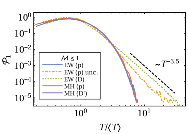
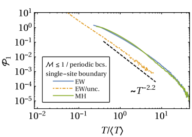
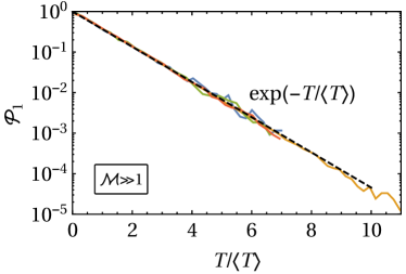
Figure 15: Probability distribution of the first-passage time $T$ (normalized by its mean value $\langle T\rangle$, see Eq. 25) in (a,b) the transient regime and (c) the equilibrium regime. In (a), the curve labeled by ‘unc.’ correspond to EW dynamics in the absence of condition (10), i.e., without the mass constraint [Eq. 9]. In (b), the absorbing boundary condition acts only on a single monomer (at location $x_{M}$) instead of the whole profile. The dash-dotted curve corresponds to EW dynamics without the mass constraint [i.e., Eq. 10 is not imposed]. In (c) the different curves, which all superimpose onto the function $\mathcal{P}_{1}\simeq\langle T\rangle\exp(-T/\langle T\rangle)$, correspond to EW and MH dynamics with periodic and Dirichlet (no-flux) boundary conditions.

The distribution $\mathcal{P}_{1}(T)$ of the first-passage time to the height $M$ obtained in the transient regime is illustrated in Fig. 15. Note that $T$ is normalized here by the mean first-passage time $\langle T\rangle$, which is discussed separately in Section III. We find that $\mathcal{P}_{1}$ generally exhibits a well-defined maximum for $T\simeq\langle T\rangle$. In the case of MH dynamics, which conserves mass [see Eq. 9], $\mathcal{P}_{1}$ decays exponentially. This is also found in the case of EW dynamics with periodic boundary conditions, in which case mass conservation is explicitly enforced via Eq. 10. In contrast, if Eq. 10 is not imposed [curve in Fig. 15 labeled by ‘unc.’], the first-passage distribution decays algebraically for large $T$, $\mathcal{P}_{1}\sim T^{-n}$, with $n\simeq 3.5$ . A similar algebraic decay is also observed in the case of EW dynamics with Dirichlet boundary conditions, where mass is conserved only as a time average.

The behavior of $\mathcal{P}_{1}$ is also sensitive to the spatially extended character of the absorbing boundary condition [see Eq. 11]. This is illustrated in Fig. 15, which shows $\mathcal{P}_{1}$ obtained in the transient regime for an absorbing boundary acting only on the monomer at $x_{M}$. Compared to Fig. 15, $\mathcal{P}_{1}$ decays here slower for large $T$, although still approximately exponentially. Lifting, in the case of EW dynamics, additionally the mass constraint results in an algebraic decay, $P_{1}\sim T^{-n}$ with $n\simeq 2.2$. This value of $n$ is smaller than the one obtained in the case of a spatially extended absorbing boundary [see Fig. 15(a)]. It is, however, close to the prediction $n\simeq 2.5$ given in Ref. Krug et al. (1997), where the transient persistence probability of an interface has been investigated.

In the equilibrium regime [see Fig. 15(b)], both for the EW and MH equation as well as for all considered boundary conditions, we empirically find that the first-passage distribution is a simple exponential function of $T/\langle T\rangle$:

$$\mathcal{P}_{1}(T)\simeq\langle T\rangle\exp(-T/\langle T\rangle).$$ (57)

The exponential behavior is in fact characteristic for a fractional Brownian walker in a parabolic potential Sliusarenko et al. (2010) and found to persist also if the absorbing boundary condition acts only on a single monomer (data not shown). Removing the mass constraint in the equilibrium regime results in a simple diffusive motion of the center-of-mass of the profile, which then dominates the first-passage distribution.

Appendix B Equilibrium distribution of height fluctuations

B.1 Periodic boundary conditions

The friction and noise parameters $\eta$ and $D$ in Eqs. 1 and 2 can be determined by requiring that the ensuing steady-state probability distribution of the profile $h(x)$ is characterized by a certain temperature $\Theta$. For periodic boundary conditions, Eqs. 1 and 2 yield in the steady-state a Gaussian joint-probability distribution of the form Majumdar and Comtet (2005); Majumdar and Dasgupta (2006)

$$P_{\text{eq}}^{\text{(p)}}[h]\sim\exp\left[-\frac{1}{4\Theta}\int_{0}^{L}\mathrm{d}x\left(\frac{\mathrm{d}h}{\mathrm{d}x}\right)^{2}\right]\,\delta[h(0)-h(L)]\,\delta\left[\int_{0}^{L}\mathrm{d}xh(x)\right],$$ (58)

with the temperature [see Eq. 19]

$$\Theta\equiv\frac{D}{2\eta}$$ (59)

in units of $k_{B}$. In Eq. 58, the $\delta$-functions enforce the periodic boundary conditions and the zero-mass constraint [Eq. 9]. The stationary single-site height distribution resulting from Eq. 58 is given by Majumdar and Comtet (2005); Majumdar and Dasgupta (2006); Foltin et al. (1994)

$$P_{\text{eq}}^{\text{(p)}}(h)=\sqrt{\frac{3}{\pi\Theta L}}\exp\left(-\frac{3}{\Theta L}h^{2}\right)\,,$$ (60)

implying the variance [see also Eq. 126]

$$\langle h^{2}\rangle=\frac{\Theta L}{6}.$$ (61)

According to Eq. 58, a profile $h(x)$ in equilibrium can be considered as a Brownian motion process for which $x$ plays the role of time. Since the motion is required to start and end here at the same point, $h(0)=h(L)$, the process is in fact a Brownian bridge, with the additional constraint of having zero area under it Majumdar and Orland (2015); Mazzolo (2017). Equation 59 is taken as a definition of the temperature throughout the present study, despite the fact that, for non-periodic boundary conditions, the resulting steady-state variance is different from Eq. 61.

B.2 Dirichlet boundary conditions

The steady-state distribution for Dirichlet boundary conditions is given by the same expression as in Eq. 58, except that $\delta[h(0)-h(L)]$ is replaced by $\delta[h(0)]\delta[h(L)]$ and that the mass constraint is present only for Dirichlet no-flux boundary conditions [see Eqs. 6 and 7]. Correlation functions can be readily determined with the aid of the closely-related propagator for a Brownian particle with fixed endpoints Chaichian and Demichev (2001); Majumdar (2005):

$$G(h,x|h_{0},x_{0})=\int_{h(0)=h_{0}}^{h(x)=h}\mathcal{D}h(\xi)\,\exp\left[-\frac{1}{4\Theta}\int_{x_{0}}^{x}\mathrm{d}\xi\left(\frac{\mathrm{d}h(\xi)}{\mathrm{d}\xi}\right)^{2}\right]=\frac{1}{\sqrt{4\pi\Theta(x-x_{0})}}\exp\left[-\frac{(h-h_{0})^{2}}{4\Theta(x-x_{0})}\right].$$ (62)

If, in addition to the endpoints also the area under the profile is constrained, corresponding to Dirichlet no-flux boundary conditions, the propagator is instead given by Majumdar and Comtet (2005); Burkhardt (1993)

$$G(h,x,A|h_{0},x_{0},A_{0})=\int_{h(0)=h_{0}}^{h(x)=h}\mathcal{D}h(\xi)\,\delta\left(\int_{x_{0}}^{x}\mathrm{d}\xi h(\xi)-A\right)\,\exp\left[-\frac{1}{4\Theta}\int_{x_{0}}^{x}\mathrm{d}\xi\left(\frac{\mathrm{d}h(\xi)}{\mathrm{d}\xi}\right)^{2}\right]\\ =\frac{\sqrt{3}}{2\pi\Theta(x-x_{0})^{2}}\exp\left[-\frac{1}{\Theta}\left(\frac{3}{(x-x_{0})^{3}}\left\{A-A_{0}-(x-x_{0})h\right\}\left\{A-A_{0}-(x-x_{0})h_{0}\right\}+\frac{1}{x-x_{0}}(h-h_{0})^{2}\right)\right].$$ (63)

$G(h,A,x|h_{0},x_{0},A_{0})$ represents the joint probability to observe a Brownian particle at location $(h,x)$, having covered the area $A=A_{0}+\int_{x_{0}}^{x}\mathrm{d}x\,h(x)$, given that the particle previously was at the location $(h_{0},x_{0})$ and had covered the area $A_{0}$. In the case of standard Dirichlet boundary conditions, the equilibrium variance of a fluctuating profile is given by

$$\begin{split}\langle h^{2}(x)\rangle=\frac{\int_{-\infty}^{\infty}\mathrm{d}h^{\prime}\,G(h^{\prime},x|0,0)\,h^{\prime 2}\,G(0,L|h^{\prime},x)}{G(0,L|0,0)}=2\Theta L\frac{x}{L}\left(1-\frac{x}{L}\right),\end{split}$$ (64)

while for the averaged path, $\langle h(x)\rangle=0$. Equation 64 also represents the variance of a Brownian bridge (see, e.g., Refs. Mazzolo (2017); Szavits-Nossan and Evans (2015)). For a Dirichlet profile whose area is constrained to vanish, the averaged path results instead as

$$\langle h(x)\rangle_{A}=\frac{\int_{-\infty}^{\infty}\mathrm{d}A^{\prime}\int_{-\infty}^{\infty}\mathrm{d}h^{\prime}\,G(h^{\prime},x,A^{\prime}|0,0,0)\,h^{\prime}\,G(0,L,0|h^{\prime},x,A^{\prime})}{G(0,L,0|0,0,0)}=6\frac{A}{L}\frac{x}{L}\left(1-\frac{x}{L}\right),$$ (65)

while its variance is given by (we consider here only $A=0$, such that $\langle h(x)\rangle_{A=0}=0$)

$$\begin{split}\langle h^{2}(x)\rangle_{A=0}=\frac{\int_{-\infty}^{\infty}\mathrm{d}A^{\prime}\int_{-\infty}^{\infty}\mathrm{d}h^{\prime}\,G(h^{\prime},x,A^{\prime}|0,0,0)\,h^{\prime 2}\,G(0,L,0|h^{\prime},x,A^{\prime})}{G(0,L,0|0,0,0)}=2\Theta L\frac{x}{L}\left(1-\frac{x}{L}\right)\left(1+3\frac{x}{L}\left(\frac{x}{L}-1\right)\right).\end{split}$$ (66)

The above results rely on the Markovian nature of the respective stochastic process. In particular, the normalization in Eqs. 65 and 66 follows from the Markovian nature of the joint stochastic process $(h,A)$, i.e., $G(h,x,A|h_{0},x_{0},A_{0})=\int_{-\infty}^{\infty}\mathrm{d}A^{\prime}\int_{-\infty}^{\infty}\mathrm{d}h^{\prime}\,G(h,x,A|h^{\prime},x^{\prime},A^{\prime})G(h^{\prime},x^{\prime},A^{\prime}|h_{0},x_{0},A_{0})$ for any $x_{0}<x^{\prime}<x$.

Appendix C Averaged path for a single Brownian walker

C.1 Averaged path with constrained endpoints

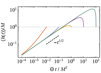
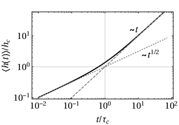
Figure 16: Averaged path $\langle h(t)\rangle_{M,T}$ [Eq. 69] of a Brownian walker starting at $(h,t)=(\epsilon,0)$ and ending at $(M>0,T>0)$ in the presence of an absorbing boundary at $h=0$. Time is made dimensionless by rescaling with $\Theta/M^{2}$. (a) Dependence of $\langle h(t)\rangle_{M,T}$ on the final time $T$ for a fixed final height $M$ (for the central endpoints from left to right: $\Theta T/M^{2}=10^{-2},10^{-1},1,10,100$). (b) Time dependence of $\langle h(t)\rangle_{M,T}$ in the regime $M^{2}\gg\Theta T$ [see Eq. 71 and the associated discussion]. The dotted and dashed lines represent the asymptotic behaviors in Eqs. 70 and 72. The characteristic length and time scales $\tau_{c}$ and $h_{c}$ are reported in Eqs. 73 and 74, respectively.

We place an absorbing boundary at height $h=0$ and consider a (Markovian) Brownian walker that departs from $(h,t)=(\epsilon,0)$ to some distant position $(M,T)$. The infinitesimal quantity $\epsilon$ is required as a regularization and the limit $\epsilon\to 0$ will be performed at the end of the calculation Redner (2001). Owing to the Markovian property of the process, the averaged trajectory of the walker can be expressed as (see also Refs. Baldassarri et al. (2003); Colaiori et al. (2004); Bhat and Redner (2015))

$$\langle h(t)\rangle_{(0,T)\to(M,T)}=\lim_{\epsilon\to 0}\frac{\int_{0}^{\infty}\mathrm{d}h\,G_{+}(M,T|h,t)\,h\,G_{+}(h,t|\epsilon,0)}{\int_{0}^{\infty}\mathrm{d}hG_{+}(M,T|h,t)G_{+}(h,t|\epsilon,0)}=\lim_{\epsilon\to 0}\frac{\int_{0}^{\infty}\mathrm{d}hG_{+}(M,T|h,t)\,h\,G_{+}(h,t|\epsilon,0)}{G_{+}(M,T|\epsilon,0)}.$$ (67)

The propagator $G_{+}(h,t|h_{0},t_{0})$ represents the conditional probability for the walker to move from $(h_{0},t_{0})$ to $(h,t)$ without $h$ becoming negative and is given by the well-known expression

$$G_{+}(h,t|h_{0},t_{0})=\frac{1}{\sqrt{4\pi\Theta(t-t_{0})}}\left[\exp\left({-\frac{(h-h_{0})^{2}}{4\Theta(t-t_{0})}}\right)-\exp\left({-\frac{(h+h_{0})^{2}}{4\Theta(t-t_{0})}}\right)\right],$$ (68)

which follows, e.g., by applying the image method to the propagator in Eq. 62 (replacing $x\to t$) Redner (2001). Equation (67) can be evaluated analytically, yielding

$$\begin{split}\langle h(t)\rangle_{M,T}&=\frac{2}{M\sqrt{\pi}}\sqrt{\Theta t\left(1-\frac{t}{T}\right)}\exp\left(\frac{M^{2}t}{4\Theta T(t-T)}\right)+\left(\frac{Mt}{T}+\frac{2d}{M}(T-t)\right)\mathrm{erf}\left[\frac{Mt}{2\sqrt{dtT(T-t)}}\right]\\ &=M\left\{\frac{2}{\sqrt{\pi}U^{2}}\sqrt{U^{2}-V^{2}}\exp\left(\frac{V^{4}}{4(V^{2}-U^{2})}\right)+\left(V^{2}+\frac{2}{V^{2}}-\frac{2}{U^{2}}\right)\mathrm{erf}\left(\frac{V^{2}}{2\sqrt{U^{2}-V^{2}}}\right)\right\},\end{split}$$ (69)

where, in the last equation, the dimensionless scaling variables $U\equiv M/\sqrt{\Theta t}$, $V\equiv M/\sqrt{\Theta T}$ have been introduced. The behavior of the averaged path is illustrated in Fig. 16(a) as a function of $\Theta t/M^{2}=1/U^{2}$. For small times $t$, one asymptotically has

$$\langle h(t\to 0)\rangle_{M,T}\simeq 4\sqrt{\frac{\Theta}{\pi}t}+\mathcal{O}(t^{3/2}).$$ (70)

At late times ($t\simeq T$), the behavior of the averaged path depends on the value of $T$ and $M$. The associated control parameter can be determined by noting that, for $U\sim\mathcal{O}(V)$ (with $U>V$), the first term in the curly brackets in Eq. 69 is small, while the error function in Eq. 69 is approximately equal to one. Accordingly, values $\langle h\rangle_{M,T}/M\gg 1$ are possible if $V^{2}\lesssim 1$, i.e., the averaged path develops a “bow” as seen in Fig. 16(a) if

$$\frac{M^{2}}{\Theta T}\lesssim 1.$$ (71)

If, on the other hand, $M^{2}/\Theta T\gtrsim 1$, the averaged path behaves linearly for $t\simeq T$:

$$\langle h(t\to T)\rangle_{M,T}\simeq M\frac{t}{T}.$$ (72)

As shown in Appendix D, this expression, being independent of the noise $\Theta$, is simply the most-likely path of the walker [see Eq. 101]. The cross-over time $\tau_{c}$ between the two regimes can be defined as the time where the two asymptotic laws in Eqs. 70 and 72 are equal, yielding

$$\tau_{c}\simeq\frac{16\Theta T^{2}}{M^{2}\pi}.$$ (73)

The two asymptotic laws can only be distinguished as long as $\tau_{c}<T$, which gives an estimate consistent with Eq. 71. Inserting Eq. 73 into Eq. 72 yields the length scale

$$h_{c}\simeq\frac{16\Theta T}{\pi M},$$ (74)

which characterizes the range of influence of the absorbing boundary. As a reflection of the scale-free nature of the Brownian process, this length depends on coordinates ($T$ and $M$) arbitrarily far away from the boundary. The averaged path given in Eq. 69 is illustrated in Fig. 16(b) in the limit $M^{2}/\Theta T\gg 1$.

In passing, we remark that the averaged trajectory $\langle h(t)\rangle$ of a free Brownian walker (i.e., in the absence of an absorbing boundary) between two points is a straight line,

$$\langle h(t)\rangle\propto t.$$ (75)

This result follows from Eq. 67 by replacing therein $G_{+}$ by the standard diffusion propagator $G$ given in Eq. 62. For free Brownian motion, the averaged path [Eq. 75] coincides with the “classical” (most-likely) path which follows from the minimization of the corresponding action [see Eq. 101 below].

C.2 First-passage path

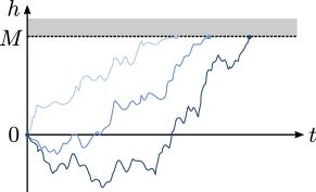
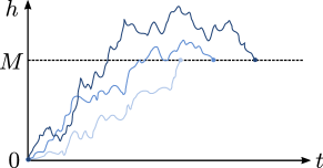
Figure 17: Transformation of the sample paths of random walkers as considered in Section C.2. (a) In the actual setup, a random walker $h(t)$ starts at the origin, $h(t=0)=0$, and moves until it hits a boundary at height $M>0$ (shaded bar) for the first time. (b) According to Eq. 76, the paths are transformed such that the first-passage event occurs at the space-time origin. In the Markovian case, the first-passage path can be directly obtained by placing an absorbing boundary at $h=0$ and considering paths that start at $h(t=0)=0$ and are conditioned to end at $h(T)=M$, with a random time $T$ governed by $F_{1}(M,T)$.

Consider a Brownian (but not necessarily Markovian) walker starting at $(h,t)=(0,0)$ in the presence of an absorbing boundary at $h=M>0$. Let $F_{1}(M,T)$ be the corresponding probability distribution of the first-passage time $T$ to the height $M$ (see below) and $\langle h(t)\rangle_{M,T}$ be the averaged path between the (fixed) points $(0,0)$ and $(M,T)$. We then define the averaged “first-passage path” of the walker, i.e., its averaged path near the first-passage event (see also Ref. Bhat and Redner (2015)), by

$$\langle h(t)\rangle=M-\frac{\int_{t}^{\infty}\mathrm{d}T\,F_{1}(M,T)\langle h(T-t)\rangle_{M,T}}{\int_{t}^{\infty}\mathrm{d}T\,F_{1}(M,T)}.$$ (76)

The associated transformation of the sample paths is illustrated in Fig. 17. Exact analytical expressions for $F_{1}$ and $\langle h(t)\rangle_{M,T}$ are available only for Markovian Brownian walkers [see Eqs. 69 and 78]. In the non-Markovian case, we shall therefore resort to numerical calculations.

C.2.1 Markovian case

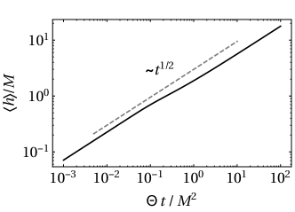
Figure 18: Markovian Brownian motion: (a) Scaling function $\mathfrak{f}_{1}$ [Eq. 79] of the first-passage distribution as a function of $\tau\equiv\Theta T/M^{2}$. The maximum occurs at $\tau=1/6$. (b) Averaged first-passage path $\langle h(t)\rangle$ [Eq. 82] of a Markovian Brownian walker in the presence of an absorbing boundary at $h=0$.

In the Markovian case, the mapping implied by Eq. 76 can be implemented by placing an absorbing boundary at $h=0$ and considering a walker which starts at $(\epsilon,0)$ (with infinitesimal $\epsilon>0$) and ends at $(M,T)$ at a random time $T$ governed by $F_{1}(M,T)$. Accordingly, using $\langle h(t)\rangle_{M,T}$ as defined in Eq. 67, the first-passage path in Eq. 76 reduces to

$$\langle h(t)\rangle=\frac{\int_{t}^{\infty}\mathrm{d}T\,F_{1}(M,T)\langle h(t)\rangle_{M,T}}{\int_{t}^{\infty}\mathrm{d}T\,F_{1}(M,T)}.$$ (77)

For a Markovian Brownian walker, the first-passage time $T$ from $h=0$ to a height $h=M$ is governed by the probability distribution Redner (2001)

$$F_{1}(M,T)=\frac{\Theta|M|}{\sqrt{4\pi\Theta T^{3}}}\exp\left(-\frac{M^{2}}{4\Theta T}\right)=\frac{M^{2}}{\Theta}\mathfrak{f}_{1}(\Theta T/M^{2}),$$ (78)

where in the last equation the scaling function

$$\mathfrak{f}_{1}(\tau)=\frac{\exp\left(-1/4\tau\right)}{\sqrt{4\pi\tau^{3}}}$$ (79)

has been introduced. For $G_{+}$ as defined in Eq. 68, one has $\int_{0}^{\infty}\mathrm{d}t\,G_{+}(\epsilon,t|M,0)=\epsilon/\Theta$, implying

$$F_{1}(M,T)=\lim_{\epsilon\to 0}\frac{\Theta}{\epsilon}G_{+}(\epsilon,T|M,0).$$ (80)

Furthermore, noting $\int_{0}^{\infty}\mathrm{d}T\,F_{1}(M,T)=1$, the quantity

$$\int_{t}^{\infty}\mathrm{d}T\,F_{1}(M,T)=1-\int_{0}^{t}\mathrm{d}T\,F_{1}(M,T)=\mathrm{erf}\left(\frac{M}{2\sqrt{\Theta t}}\right)$$ (81)

represents the survival probability. Using Eq. 81 as well as Eqs. 67 and 80, the first-passage path defined in Eq. 77 can be calculated analytically:

$$\begin{split}\langle h(t)\rangle&=\frac{1}{\int_{t}^{\infty}\mathrm{d}T\,F_{1}(M,T)}\lim_{\epsilon\to 0}\frac{\Theta}{\epsilon}\int_{0}^{\infty}\mathrm{d}h\int_{t}^{\infty}\mathrm{d}T\,G_{+}(h,t|\epsilon,0)\,h\,G_{+}(M,T|h,t)\\ &=M\left\{\frac{1+\frac{4}{\xi\sqrt{\pi}}\left[1-\exp\left(-\xi^{2}/4\right)\right]}{\mathrm{erf}\left(\xi/2\right)}-1\right\},\qquad\xi\equiv\frac{M}{\sqrt{\Theta t}},\end{split}$$ (82)

where the integral over $T$ has been performed before the one over $h$. Note that the term in the curly brackets is solely a function of the scaling variable $\xi$. For small $t$, i.e., near the absorbing boundary, Eq. 82 reduces to

$$\langle h(t\to 0)\rangle\simeq 4\sqrt{\frac{\Theta t}{\pi}}.$$ (83)

The essential reason for recovering in Eq. 83 the asymptotic behavior of the path with fixed endpoints $\langle h(t)\rangle_{M,T}$ [see Eq. 70] is that, very close to the absorbing boundary, $\langle h(t)\rangle_{M,T}$ is independent of the final time $T$ and thus can be moved out of the integral in Eq. 77 in this limit. For $\Theta t/M^{2}\gg 1$, i.e., far from the absorbing boundary, the first-passage path behaves as

$$\langle h(t)\rangle\simeq\sqrt{\pi\Theta t}.$$ (84)

The non-monotonic behavior of the path $\langle h(t)\rangle_{M,T}$ [Eq. 69] for $t$ near $T$ [see Fig. 16(a)] is reflected by a gentle “bump” of the first-passage path for $\Theta t/M^{2}\simeq 1$ [see Fig. 18(b)]. Overall, the asymptotic trajectory of a Brownian walker to its first passage point however remains at all times close to a power-law, $\langle h(t)\rangle\sim t^{1/2}$.

Note that, in the weak-noise limit ($\Theta\to 0$), the first-passage path [Eq. 82] vanishes. This is in contrast to the path with fixed endpoints [Eq. 69], for which the “classical” contribution, being independent of $\Theta$, prevails as $\Theta\to 0$ [see Eq. 72 as well as Eq. 101 below]. The time-dependence of the first-passage evolution is thus an intrinsic finite-noise property. According to Eq. 84, this applies even far from the absorbing boundary.

C.2.2 Non-Markovian case

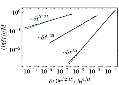
Figure 19: Numerical results (solid curves) for the averaged first-passage path $\langle h(\delta t)\rangle$ [Eq. 87] of a fractional Brownian walker approaching an absorbing boundary, for values of the Hurst index of $H=1/2$, $1/4$, and $1/8$. Note that the first-passage event occurs at $\delta t=0$ for the averaged path, i.e., $\langle h(0)\rangle=0$. The dashed curves represent the power law $C\delta t^{H}$, where the constant $C=4\sqrt{\Theta/\pi}$ follows from Eq. 83 in the case $H=1/2$, while it is obtained from a fit otherwise.

As a specific realization of a non-Markovian random walk relevant for interfacial roughening, we consider fractional Brownian motion (fBM). FBM is a Gaussian process $h(t)$ with correlation function Mandelbrot and Van Ness (1968); McCauley et al. (2007); Jeon and Metzler (2010)

$$\langle h(t)h(s)\rangle=\Theta\left(t^{2H}+s^{2H}-|t-s|^{2H}\right),$$ (85)

characterized by the Hurst index $H$. The correlation function of the relative height fluctuations $\delta h(x,t)=h(x,t)-h(x,0)$ of an equilibrated one-dimensional interface governed by Eq. 1 or (2) takes the same form as in Eq. 85 [see Eq. 18b and, e.g., Ref. Krug et al. (1997)]. Standard Markovian Brownian motion results for $H=1/2$, in which case the stochastic increments $h(t+\mathrm{d}t)-h(t)$ are uncorrelated. For $H<1/2$ ($H>1/2$), instead, the increments are anti-correlated (positively correlated). In the non-Markovian case, it is known that the distribution of the first-passage time $T$ to a single boundary asymptotically behaves as Ding and Yang (1995); Krug et al. (1997); Molchan (1999)

$$F_{1}(T\to\infty)\sim T^{-2+H}.$$ (86)

Recently, an expression for the propagator of fBM with absorption has been derived perturbatively Wiese et al. (2011); Delorme and Wiese (2016a, b). However, since closed analytical results are neither available for $F_{1}$ nor $\langle h(t)\rangle_{M,T}$, we resort in the following to numerical simulations in order to determine the first-passage path defined in Eq. 76.

We seek the averaged path of a fractional Brownian walker starting at $h(t=0)=0$ and being absorbed at a boundary at height $M>0$ [see Fig. 17(a)]. To this end, an ensemble of trajectories $\{h_{i=0,1,\ldots,N}^{(k)}\}$, each of around $N\simeq 10^{7}$ steps, are created and the step $T^{(k)}$, where $h^{(k)}_{T^{(k)}}\geq M$ for the first time, is determined for each trajectory $h^{(k)}$. Owing to the long-time tail of $F_{1}$ [see Eq. 86], the mean first passage time $\langle T\rangle$ to a single absorbing boundary is infinite. This is essentially a consequence of the fact the the walker can perform arbitrary large excursions in the negative half space ($h_{i}<0$) before hitting the boundary at $M$ Redner (2001). By checking different values of $N$ and $M$, we find that, in the present case, these excursions have negligible influence on the behavior of the averaged path near the boundary. The averaged first-passage path $\langle h_{i}\rangle$, $i=0,\ldots,N-1$ (with $i=0$ now corresponding to the first-passage event) is then obtained as

$$\langle h_{i}\rangle=N_{T\geq i}^{-1}\sideset{}{{}^{(T\geq i)}}{\sum}_{k}\left(M-h_{T^{(k)}-i}^{(k)}\right),$$ (87)

where the sum is defined to run over all $N_{T\geq i}$ paths that end at times $T\geq i$. Furthermore, the individual trajectories are shifted such that their respective first-passage times coincide (see Fig. 17).

The equivalence of Eq. 87 and Eq. 76 is readily proven: the averaged path of walkers between the fixed endpoints $(h=0,t=0)$ and $(M,T)$ is given by the restricted average $\langle h_{i}\rangle_{M,T}=\sum_{k}^{(T)}h_{i}^{(k)}/N_{T}$, where $N_{T}$ is the total number of such paths and the sum runs over precisely these paths. The discrete first-passage time distribution can be expressed as $F_{1}(M,T)=N_{T}/\sum_{T}N_{T}=N_{T}/N$, where $N$ is the total number of paths considered in the sample. Using $N_{T\geq i}=\sum_{T\geq i}N_{T}$, the discrete analogue of Eq. 76 for the averaged path can accordingly be written as

$$M-\langle h_{i}\rangle=\frac{1}{\sum_{T\geq i}F_{1}(M,T)}\sum_{T\geq i}\langle h_{T-i}\rangle_{M,T}F_{1}(M,T)=\frac{1}{\sum_{T\geq i}F_{1}(M,T)}\sum_{T\geq i}\sideset{}{{}^{(T)}}{\sum}_{k}\frac{h_{T-i}^{(k)}}{N}=\frac{1}{N_{T\geq i}}\sideset{}{{}^{(T\geq i)}}{\sum}_{k}h_{T-i}^{(k)},$$ (88)

which coincides with Eq. 87.

Simulation results obtained for the averaged first-passage path defined in Eq. 87 are shown in Fig. 19. For convenience, we revert to the notation of continuous time $\delta t$. FBM is simulated based on the “circulant method” Davies and Harte (1987); Wood and Chan (1994) (see Ref. Dieker for a practical implementation). From the plot one infers that the walker approaches the first-passage height algebraically,

$$\langle h(\delta t)\rangle\sim\delta t^{H}\,,$$ (89)

with an exponent essentially coinciding with the Hurst index $H$ of the underlying fBM process. This behavior is consistent with Eq. 83 in the Markovian case ($H=1/2$). Since $M^{2}/\Theta\sim\mathcal{O}(10^{6})$, the slight change of the logarithmic slope of the path for $H=1/2$ observed in Fig. 18(b) is only partly visible in Fig. 19. This applies also to the data for $H\neq 1/2$, if one assumes [as suggested by dimensional analysis of Eq. 85] that the crossover time generalizes to $M^{1/H}/\Theta^{1/(2H)}$ for general fBM. Note that $\langle h(\delta t)\rangle$ can be larger than $M$ for large $\delta t$ because the walker can make excursions to the lower half-space [cf. Fig. 17(a)]. Slight deviations from a pure algebraic behavior are noticeable in Fig. 19 for small times, which are found to be independent of the variance of the noise increments used in the numerical simulation as well as of the overshoot correction.

It is illuminating to consider here also the most-likely path of a fBM between two locations $h=0$ and $M$. The most-likely path minimizes the dynamic action of the associated probability functional and thus represents the weak-noise approximation of the averaged path. As shown in Appendix D, within WNT, one finds

$$h_{\text{MLP}}(\delta t)\sim\delta t^{2H}$$ (90)

near the endpoint. The different exponents in Eqs. 89 and 90 can be attributed to the repulsive effect exerted by the absorbing boundary on the fluctuations around the most-likely path (see Section VI for further discussion).

Appendix D Most-likely path of a Gaussian random process

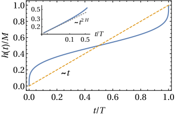
Figure 20: Most-likely path $h(t)$ of a fractional Brownian walker between the points $(h,t)=(0,0)$ and $(M,T)$ [Eq. 100]. For illustrative purposes, we have chosen a Hurst exponent of $H=1/8$. The dashed line in the main plot represents a linear path for comparison. The inset demonstrates that the asymptotic departure from the initial point follows a power-law $h(t)\propto t^{2H}$ (dashed line). A similar behavior is obtained near the final point.

We determine here the most-likely path of a Gaussian random process $h(t)$, $0\leq t\leq T$, subject to the constraints

$$h(0)=M_{0}\qquad\text{and}\qquad h(T)=M_{T},$$ (91)

where $M_{0}$ and $M_{T}$ are constants. The following discussion is in fact a straightforward application of the constrained minimization of a quadratic functional (see, e.g., Fletcher (2000)). The Gaussian process is taken to have zero mean $\langle h(t)\rangle=0$ and correlation function

$$G(t,t^{\prime})\equiv\langle h(t)h(t^{\prime})\rangle.$$ (92)

Accordingly, the joint probability distribution is given by

$$P[h]\sim\exp(-\mathcal{S}[h]),$$ (93)

with the “action”

$$\mathcal{S}[h]\equiv\frac{1}{2}\int_{0}^{T}\mathrm{d}t\int_{0}^{T}\mathrm{d}t^{\prime}\,h(t)G^{-1}(t,t^{\prime})h(t^{\prime}).$$ (94)

The inverse $G^{-1}$ of the correlation function is defined (in an operator sense) by

$$\int_{0}^{T}\mathrm{d}t\,G(s,t)G^{-1}(t,s^{\prime})=\delta(s-s^{\prime}).$$ (95)

For a Markovian process (i.e., standard Brownian motion), one has $G^{-1}(t,t^{\prime})=-\frac{1}{2}\partial_{t}^{2}\delta(t-t^{\prime})$, while the correlation function $G(t,t^{\prime})=2\text{min}(t,t^{\prime})$ Kleinert (2009). For fractional Brownian motion, the explicit form of $\mathcal{S}$ is known only perturbatively Wiese et al. (2011). In passing, we remark that the continuous time description used here should formally be understood as the limit of a multivariate Gaussian process of random variables $\{h_{i}\}$ defined at discrete times $i=0,\Delta t,\ldots,(T/\Delta t)-1$, analogously to the definition of a path integral Kleinert (2009). Imposing the constraints in Eq. 91 gives rise to the augmented action

$$\tilde{\mathcal{S}}([h],\lambda_{1},\lambda_{2})\equiv S[h]-\lambda_{1}[h(0)-M_{0}]-\lambda_{2}[h(T)-M_{T}]$$ (96)

with the Lagrange multipliers $\lambda_{1,2}$. Minimization of $\tilde{\mathcal{S}}$ with respect to $h(\tau)$ yields

$$0=\frac{\delta\tilde{\mathcal{S}}}{\delta h(\tau)}=2\int_{0}^{T}\mathrm{d}t\,h(t)G^{-1}(t,\tau)-\lambda_{1}\delta(\tau)-\lambda_{2}\delta(T-\tau),$$ (97)

where we used the symmetry property $G(t,t^{\prime})=G(t^{\prime},t)$. Multiplying Eq. 97 with the inverse correlation function $G(s,\tau)$ and integrating over $\tau$, using Eq. 95, one obtains $h(s)=\frac{1}{2}\left[G(s,0)\lambda_{1}+G(s,T)\lambda_{2}\right]$. Satisfaction of the constraints in Eq. 91 provides the values of $\lambda_{1,2}$ and eventually yields the expression of the constrained minimum-action path of a general Gaussian process (see also Ref. Norros (1999)):

$$h(s)=G(s,0)\sum_{k}(\mathbf{Q}^{-1})_{1k}M_{k}+G(s,T)\sum_{k}(\mathbf{Q}^{-1})_{2k}M_{k},$$ (98)

where

$$\mathbf{Q}\equiv\begin{pmatrix}G(0,0)&G(0,T)\\ G(T,0)&G(T,T)\end{pmatrix}$$ (99)

is the “covariance matrix of the constraints” and $\mathbf{M}\equiv(M_{0},M_{T})$. These results naturally generalize to more than two constraints. Notably, the time dependence of the minimum action path in Eq. 98 is essentially determined by the correlation function.

We now specialize the above results to fBM, i.e., a Gaussian process described by the correlation function in Eq. 85. Since this correlation function is trivially zero if one of its arguments vanishes [rendering a singular covariance matrix in Eq. 99], the evaluation of Eq. 98 is performed with a value $\epsilon>0$ instead of 0 for the initial time. After sending eventually $\epsilon\to 0$ and setting $M_{0}=0$, $M_{T}=M$ [see Eq. 91], Eq. 98 reduces to (see also Ref. Delorme and Wiese (2016a))

$$h(t)=\frac{1}{2}MT^{-2H}\left(t^{2H}-(t-T)^{2H}+T^{2H}\right),$$ (100)

where $0<t<T$. For $t\to 0$ or $t\to T$, one has $h(t)\sim t^{2H}$ and $M-h(t)\sim(T-t)^{2H}$, respectively, showing that a fractional Brownian walker approaches the endpoints of a constrained path via a power-law with exponent $2H$. This is illustrated in Fig. 20. In the Markovian case, Eq. 100 reduces to a straight line,

$$h(t)=M\frac{t}{T},\qquad(H=1/2).$$ (101)

Appendix E Review on eigenfunctions

	periodic [Eq. 103a]	Dirichlet zero $\mu$ [Eq. 103b]	Dirichlet no-flux [Eq. 103c] ($b=1$)†
$\partial_{x}^{z}$ self-adjoint	yes	yes	no
$\sigma_{k}$	$\displaystyle\frac{1}{\sqrt{L}}\exp\left(\frac{2\pi\mathrm{i}k}{L}x\right)$	$\displaystyle\sqrt{\frac{2}{L}}\sin\left(\frac{k\pi}{L}x\right)$	$\sigma_{k}^{(\mathrm{D}^{\prime})}$
$\varphi_{k}$	$\sigma_{k}$	$\sigma_{k}$	$\varphi_{k}^{(\mathrm{D}^{\prime})}$
$k$	$0,\pm 1,\pm 2,\ldots^{\ddagger}$	$1,2,3,\ldots$	$1,2,3,\ldots$
$\gamma_{k}$ [Eqs. (102), (104)]	$\displaystyle(-1)^{b+1}\left(\frac{2\pi k}{L}\right)^{z}$	$\displaystyle(-1)^{b+1}\left(\frac{k\pi}{L}\right)^{z}$	$(\omega_{k}/L)^{4}$
$\kappa_{k}$ [Eq. 107]	1	1	$\displaystyle\frac{L}{3}\left(1-\frac{(-1)^{k}}{\cosh(L\gamma_{k}^{1/4})}\right)$
$\epsilon_{k}$ [Eq. 108]	$\displaystyle\left[-|\gamma_{k}|^{1/2}\right]^{b}\kappa_{k}$, $\epsilon_{0}=0$	$\displaystyle\left[-|\gamma_{k}|^{1/2}\right]^{b}\kappa_{k}$	$-\gamma_{k}^{1/2}\kappa_{k}$

Table 1: Eigenfunctions and related properties of $\partial_{x}^{z}$ on the interval $[0,L]$ for various boundary conditions. The eigenfunctions $\sigma_{k}$ coincide with the corresponding adjoint eigenfunctions $\varphi_{k}$ if $\partial_{x}^{z}$ is self-adjoint. Furthermore, $b=0$ for EW dynamics, $b=1$ for MH dynamics, and the dynamic index $z=2b+2$. ^†Dirichlet no-flux boundary conditions are considered only for MH dynamics ($b=1$). Since $\sigma_{k}^{(\mathrm{D}^{\prime})}$ and $\varphi_{k}^{(\mathrm{D}^{\prime})}$ are not normalized here, the system size $L$ appears in the corresponding expression for $\kappa_{k}$. ^‡Due to the mass constraint [Eq. 9], the zero mode ($k=0$) is absent from the actual solution for periodic boundary conditions.

Here, a number of relevant properties of the eigenfunctions of the (bi-)harmonic operator $\partial_{x}^{z}$ on the interval $[0,L]$ are collected (see Ref. Gross (2017) for more details). We introduce a complete set of (“proper”) eigenfunctions $\sigma_{k}$, $k\in\mathbb{Z}$, fulfilling

$$\partial_{x}^{z}\sigma_{k}(x)=\gamma_{k}\sigma_{k}(x),\qquad z\in\{2,4\}$$ (102)

with eigenvalues $\gamma_{k}$. The eigenfunctions are subject to one of the following boundary conditions:

periodic: $$\sigma_{k}^{\text{(p)}}(x,t)=\sigma_{k}^{\text{(p)}}(x+L,t),$$ (103a)

Dirichlet zero-$$\mu \sigma_{k}^{(\mathrm{D})}(0,t)=0=\sigma_{k}^{(\mathrm{D})}(L,t),\qquad\partial_{x}^{2}\sigma_{k}^{(\mathrm{D})}(0,t)=0=\partial_{x}^{2}\sigma_{k}^{(\mathrm{D})}(L,t),$$: (103b)

Dirichlet no-flux: $$\sigma_{k}^{(\mathrm{D}^{\prime})}(0,t)=0=\sigma_{k}^{(\mathrm{D}^{\prime})}(L,t),\qquad\partial_{x}^{3}\sigma_{k}^{(\mathrm{D}^{\prime})}(0,t)=0=\partial_{x}^{3}\sigma_{k}^{(\mathrm{D}^{\prime})}(L,t).$$ (103c)

The symbol $\mu$ refers to the chemical potential, which vanishes at the boundary for standard Dirichlet boundary conditions (see Ref. Gross (2017)). For this reason, the latter are also called Dirichlet zero-$\mu$ boundary conditions here. Associated with $\sigma_{k}$ are a set of adjoint eigenfunctions $\varphi_{k}$, which fulfill

$$\partial_{x}^{z}\varphi_{k}(x)=\gamma_{k}\varphi_{k}(x)$$ (104)

as well as one of the following adjoint boundary conditions:

periodic: $$\varphi_{k}^{\text{(p)}}(x,t)=\varphi_{k}^{\text{(p)}}(x+L,t),$$ (105a)

Dirichlet zero-$$\mu \varphi_{k}^{(\mathrm{D})}(0,t)=0=\varphi_{k}^{(\mathrm{D})}(L,t),\qquad\partial_{x}^{2}\varphi_{k}^{(\mathrm{D})}(0,t)=0=\partial_{x}^{2}\varphi_{k}^{(\mathrm{D})}(L,t),$$: (105b)

Neumann zero-$$\mu \partial_{x}\varphi_{k}^{(\mathrm{D}^{\prime})}(0,t)=0=\partial_{x}\varphi_{k}^{(\mathrm{D}^{\prime})}(L,t),\qquad\partial_{x}^{2}\varphi_{k}^{(\mathrm{D}^{\prime})}(0,t)=0=\partial_{x}^{2}\varphi_{k}^{(\mathrm{D}^{\prime})}(L,t).$$: (105c)

Note that proper and adjoint eigenfunctions in general have an identical set of eigenvalues $\gamma_{k}$. For periodic and Dirichlet zero-$\mu$ boundary conditions, the operator $\partial_{x}^{z}$ is self-adjoint on $[0,L]$, implying that

$$\varphi_{k}^{\text{(p,D)}}=\sigma_{k}^{\text{(p,D)}}.$$ (106)

In contrast, for Dirichlet no-flux boundary conditions on $\sigma_{k}$ [Eq. 103c], the operator $\partial_{x}^{z}$ is not self-adjoint and the associated adjoint eigenfunctions $\varphi_{k}^{(\mathrm{D}^{\prime})}$ are required to satisfy the distinct boundary conditions in Eq. 105c. The eigenfunctions $\sigma_{m}$ and $\varphi_{n}$ are mutually orthogonal:

$$\int_{0}^{L}\mathrm{d}x\,\sigma_{m}^{*}(x)\varphi_{n}(x)=\kappa_{n}\delta_{mn}$$ (107)

with a real number $\kappa_{n}$. The star denotes complex conjugation, which is necessary in order to deal with complex-valued eigenfunctions, such as those for periodic boundary conditions. One furthermore has

$$\int_{0}^{L}\mathrm{d}x\,\varphi_{m}^{*}(x)\varphi_{n}^{\prime\prime}(x)=\epsilon_{n}\delta_{mn}$$ (108)

with a real number $\epsilon_{n}$. The eigenvalues of $\partial_{x}^{4}$ [see Eq. 102] for Dirichlet no-flux boundary conditions are given by

$$\gamma_{k}^{(\mathrm{D}^{\prime})}=\left(\frac{\omega_{k}^{(\mathrm{D}^{\prime})}}{L}\right)^{4},$$ (109)

where $\omega_{k}^{(\mathrm{D}^{\prime})}$ denotes a solution to the transcendental equation

$$\cos(\omega_{k}^{(\mathrm{D}^{\prime})})\cosh(\omega_{k}^{(\mathrm{D}^{\prime})})=1.$$ (110)

Numerically one obtains

$$\omega_{k}^{(\mathrm{D}^{\prime})}=4.7300,\,7.8532,\,10.9956,\ldots\qquad(k=1,2,3,\ldots)$$ (111)

Since $\sigma_{k=0}^{(\mathrm{D}^{\prime})}(x)=0$, $\sigma_{k}^{(\mathrm{D}^{\prime})}(x)=\sigma_{-k}^{(\mathrm{D}^{\prime})}(x)$, and $\omega_{k}^{(\mathrm{D}^{\prime})}=\omega_{-k}^{(\mathrm{D}^{\prime})}$, we restrict the eigenspectrum to $k\geq 1$. For $k\gtrsim 4$, an accurate approximation is provided by

$$\omega_{k}^{(\mathrm{D}^{\prime})}\simeq\pi\left(k+\frac{1}{2}\right),$$ (112)

which becomes asymptotically exact. Explicit expressions and relevant properties of $\sigma_{k}$, $\varphi_{k}$ are summarized in Table 1. (Expressions for the eigenfunctions $\sigma^{(\mathrm{D}^{\prime})}_{k}$ and $\varphi^{(\mathrm{D}^{\prime})}_{k}$ are reported Ref. Gross (2017).)

Appendix F Roughening

In the absence of an impenetrable wall, the EW and the MH equation can be solved analytically. In the context of roughening, so far mainly bulk systems or systems with periodic boundary conditions have been considered Majaniemi et al. (1996); Abraham and Upton (1989); Racz et al. (1991); Antal and Racz (1996); Barabasi and Stanley (1995); Majaniemi et al. (1996); Flekkoy and Rothman (1995, 1996); Krug (1997); Darvish and Masoudi (2009); Taloni et al. (2010b, 2012); Gross and Varnik (2013); Halpin-Healy and Zhang (1995); de Villeneuve et al. (2008). Here, we provide a general series solution in terms of the corresponding eigenfunctions, which can be readily specialized to various boundary conditions. We begin by casting Eqs. 1 and 2 into the common form

$$\partial_{t}h=(-1)^{b}\eta\partial_{x}^{z}h+\hat{\zeta}$$ (113)

with $b=0,1$ for the EW and MH equation, respectively, and $z=2b+2$. The noise $\hat{\zeta}\equiv\partial_{x}^{b}\zeta$ is correlated as [cf. Eq. 3]

$$\langle\hat{\zeta}(x,t)\hat{\zeta}(x^{\prime},t^{\prime})=(-1)^{b}2D\partial_{x}^{2b}\delta(x-x^{\prime})\delta(t-t^{\prime}).$$ (114)

To proceed, the field $h$ and the noise $\hat{\zeta}$ are expanded in terms of the eigenfunctions $\sigma_{k}(x)$ defined in Eq. 102:

$$h(x,t) =\sum_{k}h_{k}(t)\sigma_{k}(x),$$ (115a)

$$\hat{\zeta}(x,t) =\sum_{k}\hat{\zeta}_{k}(t)\sigma_{k}(x).$$ (115b)

The expansion coefficients follow from the orthogonality relation in Eq. 107 as

$$h_{k}(t) =\int_{0}^{L}\mathrm{d}x\,h(x,t)\varphi_{k}^{*}(x)/\kappa_{k},$$ (116a)

$$\hat{\zeta}_{k}(t) =\int_{0}^{L}\mathrm{d}x\,\hat{\zeta}(x,t)\varphi_{k}^{*}(x)/\kappa_{k},$$ (116b)

where $\varphi_{k}(x)$ are the adjoint eigenfunctions [Eq. 104] and $\kappa_{k}$ is reported in Table 1. Accordingly, upon using Eqs. 107 and 108, the correlation of the noise modes follows as

$$\begin{split}\langle\hat{\zeta}_{m}(t)\hat{\zeta}_{n}^{*}(t^{\prime})\rangle&=\left\langle\int_{0}^{L}\mathrm{d}x\int_{0}^{L}\mathrm{d}x^{\prime}\,\varphi_{m}^{*}(x)\varphi_{n}(x^{\prime})\partial_{x}^{b}\zeta(x,t)\partial_{x^{\prime}}^{b}\zeta(x^{\prime},t^{\prime})\frac{1}{\kappa_{m}\kappa_{n}}\right\rangle\\ &=(-1)^{b}2D\delta(t-t^{\prime})\frac{\tilde{\epsilon}_{m}}{\kappa_{m}^{2}}\delta_{mn},\end{split}$$ (117)

where $\tilde{\epsilon}_{k}\equiv\kappa_{k}$ for $b=0$ and $\tilde{\epsilon}_{k}\equiv\epsilon_{k}$ for $b=1$. The partial integrations required in the case $b=1$ have generated the factor $(-1)^{b}$ in the last line of Eq. 117; the same result is obtained upon using Eq. 114. All boundary terms vanish for the boundary conditions considered here. The mass-conserving property of the noise for MH dynamics ($b=1$) is reflected in Eq. 117 by the fact that $\tilde{\epsilon}_{0}/\kappa_{0}^{2}=0$ in this case (see Table 1) . For EW dynamics, instead, $\tilde{\epsilon}_{0}/\kappa_{0}^{2}=1$, such that the noise in principle contributes to the zero mode. Upon inserting the expansions given in Eq. 115 into Eq. 113 and using Eq. 102, one obtains

$$\partial_{t}h_{m}(t)=-\Lambda_{m}h_{m}(t)+\hat{\zeta}_{m}(t),\qquad\Lambda_{m}\equiv-(-1)^{b}\eta\gamma_{m},$$ (118)

with $\Lambda_{m}\geq 0$ and the eigenvalues $\gamma_{m}$ (see Table 1). For an arbitrary initial profile $h_{m}(0)$, the solution of Eq. 118 is given by

$$h_{m}(t)=e^{-\Lambda_{m}t}\left(h_{m}(0)+\int_{0}^{t}\mathrm{d}t^{\prime}e^{\Lambda_{m}t^{\prime}}\hat{\zeta}_{m}(t^{\prime})\right).$$ (119)

For the EW equation with periodic boundary conditions, the zero mode $h_{m=0}$ (for which $\Lambda_{0}=0$) is absent from the spectrum due to the mass constraint [Eq. 9] enforced by Eq. 10. The dynamics of $h_{0}$ obtained in the case of an unconstrained profile is discussed separately below [see Eq. 141]. In the long-time, equilibrium limit, the equal-time correlation function follows as

$$\langle h_{m}(t)h_{n}^{*}(t)\rangle\Big{|}_{t\to\infty}=\frac{D(-1)^{b}\tilde{\epsilon}_{m}}{\Lambda_{m}\kappa_{m}^{2}}\delta_{mn}\equiv V_{m}\delta_{mn}.$$ (120)

Note that $V_{m}=D|\tilde{\epsilon}_{m}|/|\Lambda_{m}|\kappa_{m}^{2}\geq 0$, as is readily shown using Table 1. Equation 120 does not apply to a zero mode, in which case Eq. 119 directly yields $\langle h_{0}(t)h_{n}^{*}(t)\rangle=0$ for all $n$ [see also Eq. 117].

Assuming uncorrelated initial conditions, $\langle h_{m}(0)h_{n}^{*}(0)\rangle\propto\delta_{mn}$, the two-time correlation function of a relative height fluctuation $\delta h_{m}(t)\equiv h_{m}(t)-h_{m}(0)$ follows from Eq. 119 as

$$\begin{split}\langle\delta h_{m}(t)\delta h_{n}^{*}(s)\rangle&=\Big{\{}\langle|h_{m}(0)|^{2}\rangle\left[1-e^{-\Lambda_{m}t}+1-e^{-\Lambda_{m}s}-\left(1-e^{-\Lambda_{m}(t+s)}\right)\right]\\ &\qquad+V_{m}\left[1-e^{-\Lambda_{m}(t+s)}-\left(1-e^{-\Lambda_{m}|t-s|}\right)\right]\Big{\}}\delta_{mn}.\end{split}$$ (121)

If the profile is initially flat, $h_{m}(0)=0$, only the second term in Eq. 121 remains:

$$\langle\delta h_{m}(t)\delta h_{n}^{*}(s)\rangle_{\text{flat}}=V_{m}\left[1-e^{-\Lambda_{m}(t+s)}-\left(1-e^{-\Lambda_{m}|t-s|}\right)\right]\delta_{mn}.$$ (122)

For thermal initial conditions, where according to Eq. 120 $\langle|h_{m}(0)|^{2}\rangle=V_{m}$, Eq. 121 instead becomes

$$\langle\delta h_{m}(t)\delta h_{n}^{*}(s)\rangle_{\text{th}}=V_{m}\left[1-e^{-\Lambda_{m}t}+1-e^{-\Lambda_{m}s}-\left(1-e^{-\Lambda_{m}|t-s|}\right)\right]\delta_{mn}.$$ (123)

The real-space correlation function follows as

$$\langle\delta h(x,t)\delta h(y,s)\rangle=\sum_{m}\langle\delta h_{m}(t)\delta h_{m}^{*}(s)\rangle\sigma_{m}(x)\sigma_{m}^{*}(y),$$ (124)

where we used the fact that $h_{-k}=h_{k}^{*}$ for periodic boundary conditions, which is a consequence of $h(x,t)$ being real.

For $t=s$ and $x=y$, the real-space correlation function reduces, both for flat and thermal initial conditions, in the long-time limit to

$$\langle|\delta h(x)|^{2}\rangle_{\text{eq}}\equiv\langle|\delta h(x,t)|^{2}\rangle_{t\to\infty}=\sum_{m}V_{m}|\sigma_{m}(x)|^{2}.$$ (125)

For periodic boundary conditions (see Table 1), one has $|\sigma_{m}(x)|^{2}=1/L$, and Eq. 125 becomes [see also Eq. 61]

$$\langle|\delta h^{\text{(p)}}|^{2}\rangle_{\text{eq}}=\frac{DL}{(2\pi)^{2}\eta}\sum_{m,m\neq 0}\frac{1}{m^{2}}=\frac{DL}{12\eta}=\frac{\Theta L}{6},$$ (126)

where we used Gradshteyn and Ryzhik (2014) $\sum_{m=1}^{\infty}m^{-2}=\pi^{2}/6$ and introduced the temperature $\Theta=D/(2\eta)$ according to Eq. 19. For Dirichlet zero-$\mu$ boundary conditions, instead, Eq. 125 becomes [see also Eq. 64]

$$\langle|\delta h^{(\mathrm{D})}(x)|^{2}\rangle_{\text{eq}}=\frac{2DL}{\pi^{2}\eta}\sum_{k=1}^{\infty}\frac{1}{k^{2}}\sin^{2}\left(\frac{k\pi x}{L}\right)=2\Theta L\frac{x}{L}\left(1-\frac{x}{L}\right),$$ (127)

where we used $\sin^{2}(y)=[1-\cos(2y)]/2$ and well-known Fourier series representations of trigonometric functions Gradshteyn and Ryzhik (2014). In the case of Dirichlet no-flux boundary conditions, instead of directly calculating the infinite sum in Eq. 125, we invoke a mapping to Brownian motion, which according to Eq. 66 yields

$$\langle|\delta h^{(\mathrm{D}^{\prime})}(x)|^{2}\rangle_{\text{eq}}=2\Theta L\frac{x}{L}\left(1-\frac{x}{L}\right)\left(1+3\frac{x}{L}\left(\frac{x}{L}-1\right)\right).$$ (128)

This expression is found to numerically coincide with Eq. 125.

For $x=y$, but arbitrary times, Eq. 124 becomes

$$\langle\delta h(x,t)\delta h(x,s)^{*}\rangle_{\text{flat}} =\mathcal{C}(t+s,x)-\mathcal{C}(|t-s|,x),$$ (129a)

$$\langle\delta h(x,t)\delta h(x,s)^{*}\rangle_{\text{th}} =\mathcal{C}(t,x)+\mathcal{C}(s,x)-\mathcal{C}(|t-s|,x),$$ (129b)

with

$$\mathcal{C}(t,x)\equiv\sum_{k}V_{k}\left(1-e^{-\Lambda_{k}t}\right)|\sigma_{k}(x)|^{2}.$$ (130)

The roughness of an interface is defined as one of the following equal time correlation functions:

$$\langle|\delta h(x,t)|^{2}\rangle_{\text{flat}} =\mathcal{C}(2t,x),$$ (131a)

$$\langle|\delta h(x,t)|^{2}\rangle_{\text{th}} =2\mathcal{C}(t,x).$$ (131b)

The finiteness and the discreteness of the system imply the existence of a smallest and a largest mode index, $k_{\text{min}}$ and $k_{\text{max}}$. In order to obtain a closed expression for the correlation function $\mathcal{C}(t,x)$, we replace the sum in Eq. 130 by an integral. The error arising from this approximation is small if the summands in Eq. 130 vary significantly only over a few $k$. This, in turn, applies if the system size is large and $t\ll 1/\Lambda_{k_{\text{min}}}$, since then the variation occurs for large $k$, where $\Lambda_{k}\sim k^{z}$. For periodic boundary conditions one has $k_{\text{min}}^{\text{(p)}}=1$ and $k_{\text{max}}^{\text{(p)}}=\lceil(L/\Delta x-1)/2\rceil$ (see Table 1 as well as Section G.1), such that Eq. 130 becomes

$$\mathcal{C}^{\text{(p)}}(t)\simeq\frac{D}{\eta\pi}\int_{p^{\text{(p)}}_{\text{min}}}^{p^{\text{(p)}}_{\text{max}}}\mathrm{d}p\frac{1-\exp(-\eta p^{z}t)}{k^{2}}\equiv\mathcal{C}(t;p^{\text{(p)}}_{\text{min,max}}),$$ (132)

where we introduced the wave number $p^{\text{(p)}}\equiv 2\pi k^{\text{(p)}}/L$ associated with $k$. Note that Eq. 132 is independent of $x$ owing to translational invariance. For standard Dirichlet boundary conditions, instead, one has $k_{\text{min}}^{\text{(D)}}=1$ and $k_{\text{max}}^{\text{(D)}}=L/\Delta x-1$ (see Section G.1]). In order to evaluate Eq. 130, we focus on the point $x=L/2$ and note that $\sqrt{L/2}\,\sigma_{k}(L/2)=1,0,-1,0,1,\ldots$ for $k=1,2,3,\ldots$, such that one obtains

$$\begin{split}\mathcal{C}^{(\mathrm{D})}(t,L/2)&=\frac{2D}{\eta L}\sum_{n=0}^{n_{\text{max}}}\frac{1-\exp(-\eta[(2n+1)\pi/L]^{z}t)}{[(2n+1)\pi/L]^{2}}\simeq\frac{D}{\eta\pi}\int_{p_{\text{min}}^{(\mathrm{D})}}^{p_{\text{max}}^{(\mathrm{D})}}\mathrm{d}p\frac{1-\exp(-\eta p^{z}t)}{p^{2}}\\ &=\mathcal{C}(t;p_{\text{min,max}}^{(\mathrm{D})}),\end{split}$$ (133)

where $n\equiv 2k+1$, $n_{\text{max}}\equiv\lceil(L/\Delta x-1)/2\rceil$, and $p^{(\mathrm{D})}\equiv\pi k^{(\mathrm{D})}/L$. For Dirichlet no-flux boundary conditions and a sufficiently large integer $k^{\prime}$, one may approximate, for $k\geq k^{\prime}$, $|\Lambda_{k}|/\eta\simeq((k+1/2)\pi/L)^{4}$, $[\sigma^{(\mathrm{D}^{\prime})}_{k}(L/2)]^{2}\simeq 2/3$ for even $k$, while $\sigma^{(\mathrm{D}^{\prime})}_{k}(L/2)=0$ for odd $k$ (see Table 1 and Ref. Gross (2017)). Leaving at this point the largest mode $k_{\text{max}}^{(\mathrm{D}^{\prime})}$ unspecified , we accordingly obtain ($n\equiv k/2$)

$$\mathcal{C}^{(\mathrm{D}^{\prime})}(t,L/2)\simeq\frac{2D}{\eta L}\sum_{n=\lfloor k^{\prime}/2\rfloor}^{\lceil k_{\text{max}}^{(\mathrm{D}^{\prime})}/2\rceil}\frac{1-\exp(-\eta[2\pi n/L+\pi/2L]^{4}t)}{(2\pi n/L+\pi/2L)^{2}}\simeq\mathcal{C}(t;p_{\text{min,max}}^{(\mathrm{D}^{\prime})})$$ (134)

with $p_{\text{max}}^{(\mathrm{D}^{\prime})}=(k_{\text{max}}^{(\mathrm{D}^{\prime})}+1/2)\pi/L$. The freedom in the choice for the lower bound $k^{\prime}$ leads to a negligible error in $\mathcal{C}^{(\mathrm{D}^{\prime})}$ at large times. We thus re-instate for the smallest wave number the exact value $p_{\text{min}}^{(\mathrm{D}^{\prime})}=\omega_{1}^{(\mathrm{D}^{\prime})}/L$, with $\omega_{1}^{(\mathrm{D}^{\prime})}$ defined in Eq. 111. In conclusion, the expression for $\mathcal{C}(t;p_{\text{min,max}})$ in Eq. 132, which approximates the one-point correlation function in Eq. 130 at $x=L/2$, depends on the boundary conditions only via the integration boundaries $p_{\text{min,max}}$. The integral in Eq. 132 can be calculated in closed form, leading to

$$\mathcal{C}(t)=\frac{D}{\eta\pi}(\eta t)^{\frac{1}{z}}z^{-1}\int_{\eta tp_{\text{min}}^{z}}^{\eta tp_{\text{max}}^{z}}\mathrm{d}x\,x^{-\frac{1}{z}-1}\left(1-e^{-x}\right)=\frac{D}{\eta\pi}(\eta t)^{1/z}z^{-1}\left[\Gamma\left(-z^{-1},x\right)-zx^{-1/z}\right]_{x=\eta tp_{\text{min}}^{z}}^{x=\eta tp_{\text{max}}^{z}},$$ (135)

with $\Gamma(n,x)$ being the upper incomplete Gamma-function. To proceed, we introduce the crossover time $\tau_{\times}=1/(\eta p_{\text{max}}^{z})$, as well as the roughening time

$$\tau_{R}=\begin{cases}\displaystyle\left(\frac{L}{2\pi}\right)^{z}\frac{1}{\eta},\qquad&\text{periodic},\\ \displaystyle\left(\frac{L}{\pi}\right)^{z}\frac{1}{\eta},\qquad&\text{standard Dirichlet},\\ \displaystyle\left(\frac{L}{\omega_{1}^{(\mathrm{D}^{\prime})}}\right)^{z}\frac{1}{\eta},\qquad&\text{Dirichlet no-flux boundary conditions},\end{cases}$$ (136)

for which one has $\tau_{R}\simeq 1/(\eta p_{\text{min}}^{z})$ [see also Eqs. 14 and 15]. From Eq. 118 one infers that $\tau_{R}$ and $\tau_{\times}$ are the relaxation times of the mode with largest and smallest wavelength that can be accommodated by the system. The correlation function $\mathcal{C}(t)$ exhibits three distinct asymptotic regimes:

$$\mathcal{C}(t)\simeq\frac{2\Theta}{\pi}\begin{cases}\displaystyle\frac{p_{\text{max}}^{z-1}-p_{\text{min}}^{z-1}}{z-1}t,\quad&t\lesssim\tau_{\times},\\ \Gamma\left(1-z^{-1}\right)(\eta t)^{1/z},&\tau_{\times}\lesssim t\lesssim\tau_{R},\\ \frac{1}{p_{\text{min}}}-\frac{1}{p_{\text{max}}},&t\gtrsim\tau_{R},\end{cases}$$ (137)

i.e., an initial diffusive growth followed by a subdiffusive law characterized by the dynamic index $z$. For times of the order of $\tau_{R}$, the height variance saturates to its equilibrium value . In the subdiffusive regime, the two-time correlation functions in Eq. 129, evaluated for $x=L/2$, take the form Krug et al. (1997); Taloni et al. (2012)

$$\langle\delta h(x,t)\delta h(x,s)^{*}\rangle_{\text{flat}} \simeq(2\Theta/\pi)\eta^{1/z}\Gamma(1-z^{-1})\left[(t+s)^{1/z}-|t-s|^{1/z}\right],$$ (138a)

$$\langle\delta h(x,t)\delta h(x,s)^{*}\rangle_{\text{th}} \simeq(2\Theta/\pi)\eta^{1/z}\Gamma(1-z^{-1})\left[t^{1/z}+s^{1/z}-|t-s|^{1/z}\right].$$ (138b)

Note that the prefactors in the above expression will be different if $x\neq L/2$. Recalling that the height fluctuations are Gaussian, Eq. 138b shows that, in the equilibrium regime, a tagged monomer of a one-dimensional profile performs a fractional Brownian motion [cf. Eq. 85] with Hurst index Krug et al. (1997)

$$H=\frac{1}{2z}.$$ (139)

In contrast, in the transient roughening regime, the correlation function in Eq. 138a describes a non-Markovian Gaussian process with non-stationary increments. In the subdiffusive regime, a tagged monomer $h(x,t)$ traverses a distance $\Delta$ within a characteristic diffusion time $\tau_{D}$ determined by $\Delta\simeq\langle\delta h(x,\tau_{D})^{2}\rangle^{1/2}$. Equation 138, which applies to $x\simeq L/2$ , yields accordingly

$$\tau_{D}\simeq\frac{\Delta^{2z}}{[(2/\pi)\Theta\Gamma(1-z^{-1})]^{z}c\eta},$$ (140)

with $c=2$ for flat initial conditions and $c=2^{z}$ for thermal ones. Within a time $\tau_{R}$, a tagged monomer has covered a region of a typical extent set by the equilibrium variance, $\langle h^{2}\rangle^{1/2}$ [see Eqs. 126 to 128].

For EW dynamics with periodic boundary conditions, the zero-mode ($k=0$) is absent from Eq. 119 as a consequence of enforcing the mass constraint [see Eqs. 9 and 10]. Without this constraint, the two-time correlation function of $h_{0}$ [cf. Eq. 120] results as

$$\langle h_{0}(t)h_{0}^{*}(s)\rangle=2D\,\text{min}(t,s),$$ (141)

representing standard Brownian diffusion of the center-of-mass of the profile.

Appendix G Numerical implementation of the Langevin simulations

G.1 Discretization

Figure 21: On a one-dimensional lattice of $N$ nodes, Dirichlet boundary conditions are imposed at the nodes 0 and $N-1$ (highlighted gray), i.e., $h(x_{0})=0=h(x_{N-1})$.

As reported in Eq. 23, we use in our simulations a standard Euler discretization in time for Eqs. 1 and 2:

$$h(x_{i},t+\Delta t)=h(x_{i},t)-\eta\,\Delta t\,(-\nabla^{2})^{z/2}h(x_{i},t)+\sqrt{2D\Delta t}\nabla^{z/2-1}\zeta(x_{i},t),$$ (142)

where $i=0,1,2,\ldots,N-1$, $N=L/\Delta x$ denotes the number of lattice nodes and $\Delta x$ is the lattice spacing. For notational simplicity, here we have dropped the tilde on $\zeta$. The required spatial derivatives are discretized based on a standard central difference scheme Zwillinger (1997):

$$\nabla\zeta_{i}(x_{i}) \equiv\frac{1}{2}\left[\zeta(x_{i+1})-\zeta(x_{i-1})\right],$$ (143a)

$$\nabla^{2}h(x_{i}) \equiv h(x_{i-1})-2h(x_{i})+h(x_{i+1}),$$ (143b)

$$\nabla^{4}h(x_{i}) \equiv h(x_{i-2})-4h(x_{i-1})+6h(x_{i})-4h(x_{i+1})+h(x_{i+2}).$$ (143c)

Here and in the following, the time argument is suppressed and length is expressed in units of $\Delta x$. We remark that the discretizations for the bi-Laplacian in Eq. 143c and the Laplacian in Eq. 143b are related via $\nabla^{4}=\nabla^{2}(\nabla^{2})$. We consider periodic boundary conditions,

$$h(x_{N+i})=h(x_{i}),$$ (144)

and Dirichlet boundary conditions

$$h(x_{0})=0=h(x_{N-1}).$$ (145)

For Dirichlet boundary conditions, Eq. 142 is evaluated only at the nodes $1\leq i\leq N-2$ (see Fig. 21). Since the discretized Laplacian in Eq. 143b requires only the values of $h$ at the nearest neighbors, the boundary conditions defined in Eqs. 144 and 145 fully determine the discretized EW dynamics. In contrast, in the case of the MH equation, the discretized bi-Laplacian in Eq. 143c involves also next-nearest neighbors and is thus a priori undefined at the boundary nodes $i\in\{1,N-2\}$. For Dirichlet no-flux boundary conditions, an expression of the discretized bi-Laplacian at the boundary can be determined by requiring conservation of the total mass $\mathcal{A}=\sum_{i=1}^{N-2}h(x_{i})$ at each time step. Within the domain $2\leq i\leq N-3$, the deterministic contribution to the change of the mass, i.e., the contribution stemming from the second term on the r.h.s. of Eq. 142, is obtained as

$$\sum_{i=2}^{N-3}\nabla^{4}h(x_{i})=-3h(x_{1})+3h(x_{2})-h(x_{3})-h(x_{N-4})+3h(x_{N-3})-3h(x_{N-2}),$$ (146)

where Eqs. 143c and 145 have been used and any prefactors are omitted. Accordingly, the simplest choice for $\nabla^{4}$ at the nodes $i\in\{1,N-2\}$ ensuring vanishing of the total deterministic mass change is given by:

$$\nabla^{4}h(x_{1}) =3h(x_{1})-3h(x_{2})+h(x_{3}),$$ (147a)

$$\nabla^{4}h(x_{N-2}) =h(x_{N-4})-3h(x_{N-3})+3h(x_{N-2}).$$ (147b)

Concerning the stochastic contribution to the mass change, the last term on the r.h.s. of Eq. 142 yields

$$\sum_{i=1}^{N-2}\nabla\zeta(x_{i})=\frac{1}{2}\left[-\zeta(x_{0})-\zeta(x_{1})+\zeta(x_{N-2})+\zeta(x_{N-1})\right].$$ (148)

In order for this expression to vanish, a choice for $\zeta(x_{i})$ at the boundary nodes $i=0,N-1$ must be made. Given Eq. 145, it appears natural to set

$$\zeta(x_{0})= 0=\zeta(x_{N-1}),$$ (149a)

which, by Eq. 148, implies

$$\zeta(x_{1})= 0=\zeta(x_{N-2}).$$ (149b)

The above choice is not unique, but minimizes artificial correlations. Alternatively, one may set $\zeta(x_{0})=-\zeta(x_{1})$ and $\zeta(x_{N-1})=-\zeta(x_{N-2})$. This choice been checked in a number of cases to yield similar results to the prescription in Eq. 149. For periodic boundary conditions, finally, it is straightforward to prove that mass is exactly conserved by Eq. 142.

It can be readily shown that Eq. 147 in fact implies a vanishing (discretized) flux at the boundaries, i.e., $\nabla\mu(x_{i})=0$ for $i=1,N-2$, where

$$\mu(x_{i})\equiv-\nabla^{2}h(x_{i})=-[h(x_{i-1})-2h(x_{i})+h(x_{i+1})]$$ (150)

is the chemical potential. To this end, we introduce the forward difference

$$\nabla^{F}h(x_{i})\equiv h(x_{i+1})-h(x_{i}),$$ (151)

in terms of which the Laplacian of $\mu$ can be written as

$$\begin{split}\nabla^{2}\mu(x_{i})=-\nabla^{4}h(x_{i})&=[\mu(x_{i-1})-\mu(x_{i})]+[\mu(x_{i+1})-\mu(x_{i})]\\ &=-\nabla^{F}\mu(x_{i-1})+\nabla^{F}\mu(x_{i}),\qquad i=1,\ldots,N-1.\end{split}$$ (152)

Upon imposing no-flux boundary conditions in the discretized form

$$\nabla^{F}\mu(x_{0})=0=\nabla^{F}\mu(x_{N-2}),$$ (153)

one recovers the expressions in Eq. 147:

$$\nabla^{4}h(x_{1}) =\mu(x_{1})-\mu(x_{2}),$$ (154a)

$$\nabla^{4}h(x_{N-2}) =\mu(x_{N-2})-\mu(x_{N-3}).$$ (154b)

We finally recall some useful properties related to the eigenmode decomposition of the profile for various boundary conditions. In the case of periodic boundary conditions, $h(x)$ can be expressed in terms of its Fourier modes as

$$h^{\text{(p)}}(x)=\sum_{q=0}^{N-1}\exp\left(\frac{2\pi\mathrm{i}q}{L}x\right)h_{q}^{\text{(p)}}.$$ (155)

Correspondingly, taking into account the discrete nature of $h(x)$, the Fourier coefficients $h_{q}$ are given by

$$h_{q}^{\text{(p)}}=\frac{1}{N}\sum_{k=0}^{N-1}\exp\left(-\frac{2\pi\mathrm{i}}{L}qk\Delta x\right)h^{\text{(p)}}(k\Delta x),$$ (156)

where we reinstated the lattice spacing $\Delta x$. Note that

$$\sum_{k=0}^{N-1}\exp\left(\frac{2\pi\mathrm{i}}{N}qk\right)=N\delta_{q,N\mathbb{Z}},$$ (157)

where $\delta_{q,N\mathbb{Z}}\equiv 1$ if $q$ is an integer multiple of $N$, and zero otherwise. Since Eq. 156 implies $h_{N-q}=h_{q}^{*}$, a real-valued $h(x)$ is completely determined by its (complex) Fourier coefficients $h_{q}$ within the first Brillouin zone, $q=0,1,\ldots,\lceil(N-1)/2\rceil$, where $\lceil x\rceil$ denotes the largest integer smaller than or equal to $x$.

In the case of standard Dirichlet boundary conditions, $h(x)$ can be analogously decomposed as

$$h^{\text{(D)}}(x)=\sum_{q=0}^{N-1}\sin\left(\frac{\pi q}{L}x\right)h_{q}^{\text{(D)}},$$ (158)

with the inverse relation

$$h_{q}^{\text{(D)}}=\frac{2}{N}\sum_{k=0}^{N-1}\sin\left(\frac{\pi q}{L}k\Delta x\right)h^{\text{(D)}}(k\Delta x).$$ (159)

The orthogonality property is given by

$$\sum_{k=0}^{N-1}\sin\left(\frac{\pi p}{N}k\right)\sin\left(\frac{\pi q}{N}k\right)=\begin{cases}\frac{N}{2}\delta_{p,q},\qquad&q,p\neq 0,\\ 0,\qquad&p=q=0,\end{cases}$$ (160)

assuming $0\leq q,p\leq N-1$. Indeed, since $\sin(\pi(2N-q)k/N)=-\sin(\pi qk/N)$, the specification of the expansion coefficients $h_{q}$ for $0\leq q\leq N-1$ completely determines $h^{\text{(D)}}(x)$ on a lattice of $N=L/\Delta x$ points and, accordingly, one has $h^{\text{(D)}}_{2N-q}=-h^{\text{(D)}}_{q}$

G.2 Benchmarks

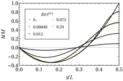
Figure 22: Deterministic relaxation of a profile with Dirichlet no-flux boundary conditions for the noiseless MH equation [see Eq. 142]. The profile is initialized with the static first-passage profile obtained within WNT in the equilibrium regime, given by Eq. I-(C63) for $\delta t=0$ and $x_{M}=L/2$. Symbols represent simulation results, while solid curves represent the time-dependent first-passage profile $h(x,\delta t)$ predicted by WNT [Eq. I-(C63)] for the same value of $x_{M}$. Time is expressed in terms of the relaxation time $\tau^{(\mathrm{D}^{\prime})}$ [Eq. 14].

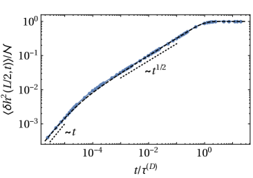
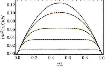
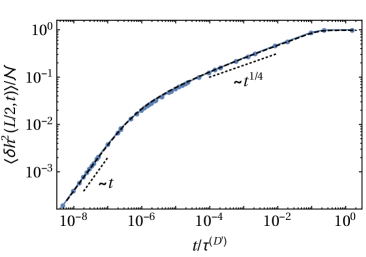
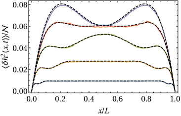
Figure 23: Non-equilibrium roughening of a profile for (a,b) EW dynamics with (standard) Dirichlet boundary conditions [Eq. 6], and (c,d) MH dynamics with Dirichlet no-flux boundary conditions [Eqs. 6 and 7]. The profile is initialized at time $t=0$ in a flat configuration [Eq. 4]. Panels (a,c) show the time evolution of the roughness $\langle|\delta h(L/2,t)|^{2}\rangle$ [Eq. 131] at the mid-point, while panels (b,d) show the roughness as a function of $x$ for various times. Simulation data are represented in (a,c) by the connected symbols and in (b,d) by the solid lines. The dotted lines in (a,c) represent power-laws expected asymptotically at early and intermediate times [see Eq. 137]. For sufficiently large system size $L$, the exponent characterizing the intermediate time regime is predicted to be $1/z$ independently from the boundary conditions. The dashed curves in (b,d) represent the analytical predictions in Eq. 131a, normalized (via the factor $\mathcal{N}$) to the corresponding long-time limits [see Eqs. 127 and 128].

We now assess the accuracy of the discretizations in Eq. 142 with a few benchmarks. Figure 22 illustrates the deterministic relaxation of a profile governed by the noiseless MH equation with Dirichlet no-flux boundary conditions. As initial configuration (at time $\delta t=0$) we take here the first-passage profile obtained from the solution of WNT in Eq. I-(3.19) for $T\to\infty$ and $x_{M}=L/2$. Since this profile pertains to the equilibrium regime, the relaxation solution shown in Fig. 22 is expected to be the identical to the time-inversed activation solution obtained within WNT for the same value of $x_{M}$. A convenient form of the activation solution, expressed in terms of the time variable $\delta t=T-t$, is provided in Eq. I-(C63). We find close agreement between the simulation results (symbols) and WNT (solid curves).

Figure 23 illustrates interfacial roughening for the EW and MH equations with Dirichlet (no-flux) boundary conditions and a flat initial configuration [Eq. 4]. Simulation results (symbols and solid lines) obtained for the time-dependent variance $\langle\delta h^{2}(x,t)\rangle$ [normalized to its long-time limit $\langle\delta h^{2}(x,t\to\infty)\rangle$] are shown in panels (a,c) as a function of time for $x=L/2$ and in panels (b,d) as a function of $x$ for various times. The dashed curves in Fig. 23 represent the analytical predictions reported in Eq. 131a [normalized to the equilibrium variance $\mathcal{N}$ given in Eqs. 127 and 128]. (We remark that, for periodic boundary conditions, the variance evolves in essentially the same fashion as in Fig. 23(a,c).) In agreement with Eq. 137, the variance grows linearly in time for $t\lesssim\tau_{\times}$, followed by an algebraic growth with exponent $1/z$ for $\tau_{\times}\lesssim t\lesssim\tau$, where $\tau_{\times}$ and $\tau$ are the crossover and the relaxation time, respectively [see Eqs. 15 and 14]. In the case of MH dynamics, the slight deviation of the simulation results from the expected value $1/4$ of the power-law exponent at intermediate times is found to gradually diminish upon increasing the system size $L$.

In order to determine the crossover time $\tau_{\times}$, recall that for standard Dirichlet boundary conditions, one has $L/\Delta x-1\simeq L/\Delta x$ distinct wavemodes ($k=1,\ldots,L/\Delta x-1$) on a lattice of size $L$ [see Eq. 160 and the related discussion]. As observed in Fig. 23(a), the resulting crossover time $\tau_{\times}$ is correctly captured by the solution in Eq. 137 (dashed curve). For Dirichlet no-flux boundary conditions, there is no symmetry between the eigenmodes $\sigma_{k}^{(\mathrm{D}^{\prime})}(x)$ [see Table 1] for small and large $k$, hence the largest possible eigenmode is not easily obtained. In order to gain further insight into this issue, we determine the stability of an eigenmode via numerical simulation. To this end, the noiseless relaxation of a profile $h(x,t)$, initialized as $h(x,0)=\sigma_{k}^{(\mathrm{D}^{\prime})}(x)$, is simulated under MH dynamics. For a system size of, e.g., $L=100\Delta x$, we find that eigenmodes with $k\lesssim L/(2\Delta x)$ typically keep their shape during the time evolution, i.e., $h(x,t)/h(x_{\text{ref}},t)\simeq\sigma_{k}^{(\mathrm{D}^{\prime})}(x)$, where $x_{\text{ref}}$ is a suitable reference position. For $k\gtrsim L/(2\Delta x)$, instead, the profile is strongly disturbed during the evolution, indicating that the corresponding eigenmode is unstable under the discretization used here. The instability is amplified upon increasing $k$. We find that, using for the evaluation of Eq. 131a a value of $k\simeq 0.6L/\Delta x$ for the largest mode number, accurately captures the crossover-time observed in Fig. 23(c).

References

- Gross (2017) M. Gross, “First-passage dynamics of linear stochastic interface models: weak-noise theory and influence of boundary conditions,” (2017).
- Edwards and Wilkinson (1982) S. F. Edwards and D. R. Wilkinson, “The Surface Statistics of a Granular Aggregate,” Proc. Roy. Soc. Lond. A. Math. Phys. 381, 17 (1982).
- Mullins (1957) W. W. Mullins, “Theory of Thermal Grooving,” J. Appl. Phys. 28, 333 (1957).
- Herring (1950) C. Herring, “Effect of Change of Scale on Sintering Phenomena,” J. Appl. Phys. 21, 301 (1950).
- Krug (1997) J. Krug, “Origins of scale invariance in growth processes,” Adv. Phys. 46, 139 (1997).
- Gross and Varnik (2013) M. Gross and F. Varnik, “Interfacial roughening in nonideal fluids: Dynamic scaling in the weak- and strong-damping regime,” Phys. Rev. E 87, 022407 (2013).
- Gardiner (2009) C. Gardiner, Stochastic Methods: A Handbook for the Natural and Social Sciences, 4th ed. (Springer, Berlin, 2009).
- Redner (2001) S. Redner, A Guide to First-Passage Processes (Cambridge University Press, 2001).
- Delfino and Squarcini (2013) G. Delfino and A. Squarcini, “Interfaces and wetting transition on the half plane. Exact results from field theory,” J. Stat. Mech. 2013, P05010 (2013).
- Belardinelli et al. (2016) D. Belardinelli, M. Sbragaglia, M. Gross, and B. Andreotti, “Thermal fluctuations of an interface near a contact line,” Phys. Rev. E 94, 052803 (2016).
- Krug et al. (1997) J. Krug, H. Kallabis, S. N. Majumdar, S. J. Cornell, A. J. Bray, and C. Sire, “Persistence exponents for fluctuating interfaces,” Phys. Rev. E 56, 2702 (1997).
- Likthman and Marques (2006) A. E. Likthman and C. M. Marques, “First-passage problem for the Rouse polymer chain: An exact solution,” EPL 75, 971 (2006).
- Guerin et al. (2012) T. Guerin, O. Benichou, and R. Voituriez, “Non-Markovian polymer reaction kinetics,” Nat. Chem. 4, 568 (2012); T. Guerin, O. Benichou, and R. Voituriez, “Reactive conformations and non-Markovian reaction kinetics of a Rouse polymer searching for a target in confinement,” Phys. Rev. E 87, 032601 (2013) .
- Bray et al. (2013) A. J. Bray, S. N. Majumdar, and G. Schehr, “Persistence and first-passage properties in nonequilibrium systems,” Adv. Phys. 62, 225 (2013).
- Cao et al. (2015) J. Cao, J. Zhu, Z. Wang, and A. E. Likhtman, “Large deviations of Rouse polymer chain: First passage problem,” J. Chem. Phys. 143, 204105 (2015).
- Meerson and Vilenkin (2016) B. Meerson and A. Vilenkin, “Macroscopic fluctuation theory and first-passage properties of surface diffusion,” Phys. Rev. E 93, 020102 (2016).
- Halpin-Healy and Zhang (1995) T. Halpin-Healy and Y.-C. Zhang, “Kinetic roughening phenomena, stochastic growth, directed polymers and all that. Aspects of multidisciplinary statistical mechanics,” Phys. Rep. 254, 215 (1995).
- Freidlin and Wentzell (1998) M. I. Freidlin and A. D. Wentzell, Random perturbations of dynamical systems, 2nd ed., Grundlehren der Mathematischen Wissenschaften [Fundamental Principles of Mathematical Sciences], Vol. 260 (Springer-Verlag, New York, 1998).
- Bertini et al. (2015) L. Bertini, A. De Sole, D. Gabrielli, G. Jona-Lasinio, and C. Landim, “Macroscopic fluctuation theory,” Rev. Mod. Phys. 87, 593 (2015).
- Bausch and Blossey (1994) R. Bausch and R. Blossey, “Lifetime of undercooled wetting layers,” Phys. Rev. E 50, R1759 (1994).
- Bausch et al. (1994) R. Bausch, R. Blossey, and M. A. Burschka, “Critical nuclei for wetting and dewetting,” J. Phys. A: Math. Gen. 27, 1405 (1994).
- Blossey (1995) R. Blossey, “Nucleation at first-order wetting transitions,” Int. J. Mod. Phys. B 09, 3489 (1995).
- Foltin et al. (1997) G. Foltin, R. Bausch, and R. Blossey, “Critical holes in undercooled wetting layers,” J. Phys. A: Math. Gen. 30, 2937 (1997).
- Seemann et al. (2001) R. Seemann, S. Herminghaus, and K. Jacobs, “Dewetting Patterns and Molecular Forces: A Reconciliation,” Phys. Rev. Lett. 86, 5534 (2001).
- Thiele et al. (2001) U. Thiele, M. G. Velarde, and K. Neuffer, “Dewetting: Film Rupture by Nucleation in the Spinodal Regime,” Phys. Rev. Lett. 87, 016104 (2001).
- Thiele et al. (2002) U. Thiele, K. Neuffer, Y. Pomeau, and M. G. Velarde, “On the importance of nucleation solutions for the rupture of thin liquid films,” Coll. Surf. A 206, 135 (2002).
- Tsui et al. (2003) O. K. C. Tsui, Y. J. Wang, H. Zhao, and B. Du, “Some views about the controversial dewetting morphology of polystyrene films,” Eur. Phys. J. E 12, 417 (2003).
- Becker et al. (2003) J. Becker, G. Grün, R. Seemann, H. Mantz, K. Jacobs, K. R. Mecke, and R. Blossey, “Complex dewetting scenarios captured by thin-film models,” Nat. Mater. 2, 59 (2003).
- Gruen et al. (2006) G. Gruen, K. Mecke, and M. Rauscher, “Thin-Film Flow Influenced by Thermal Noise,” J. Stat. Phys. 122, 1261 (2006).
- Fetzer et al. (2007) R. Fetzer, M. Rauscher, R. Seemann, K. Jacobs, and K. Mecke, “Thermal Noise Influences Fluid Flow in Thin Films during Spinodal Dewetting,” Phys. Rev. Lett. 99, 114503 (2007).
- Croll and Dalnoki-Veress (2010) A. B. Croll and K. Dalnoki-Veress, “Hole nucleation in free-standing polymer membranes: the effects of varying molecular architecture,” Soft Matter 6, 5547 (2010).
- Blossey (2012) R. Blossey, Thin Liquid Films, Theoretical and Mathematical Physics (Springer Netherlands, Dordrecht, 2012).
- Nguyen et al. (2014) T. D. Nguyen, M. Fuentes-Cabrera, J. D. Fowlkes, and P. D. Rack, “Coexistence of spinodal instability and thermal nucleation in thin-film rupture: Insights from molecular levels,” Phys. Rev. E 89, 032403 (2014).
- Duran-Olivencia et al. (2017) M. A. Duran-Olivencia, R. S. Gvalani, S. Kalliadasis, and G. A. Pavliotis, “Instability, rupture and fluctuations in thin liquid films: Theory and computations,” arXiv:1707.08811 (2017).
- Lekkerkerker et al. (2008) H. N. W. Lekkerkerker, V. W. A. d. Villeneuve, J. W. J. d. Folter, M. Schmidt, Y. Hennequin, D. Bonn, J. O. Indekeu, and D. G. A. L. Aarts, “Life at ultralow interfacial tension: wetting, waves and droplets in demixed colloid-polymer mixtures,” Eur. Phys. J. B 64, 341 (2008).
- Aarts and Lekkerkerker (2008) D. G. A. L. Aarts and H. N. W. Lekkerkerker, “Droplet coalescence: drainage, film rupture and neck growth in ultralow interfacial tension systems,” J. Fluid Mech. 606, 275 (2008).
- Eggers (2002) J. Eggers, “Dynamics of Liquid Nanojets,” Phys. Rev. Lett. 89, 084502 (2002).
- Petit et al. (2012) J. Petit, D. Rivière, H. Kellay, and J.-P. Delville, “Break-up dynamics of fluctuating liquid threads,” Proc. Natl. Acad. Sci. 109, 18327 (2012).
- Hennequin et al. (2006) Y. Hennequin, D. G. A. L. Aarts, J. H. van der Wiel, G. Wegdam, J. Eggers, H. N. W. Lekkerkerker, and D. Bonn, “Drop Formation by Thermal Fluctuations at an Ultralow Surface Tension,” Phys. Rev. Lett. 97, 244502 (2006).
- Mo et al. (2015) C.-j. Mo, L.-j. Yang, F. Zhao, and K.-d. Cui, “Mesoscopic simulation of a thinning liquid bridge using the dissipative particle dynamics method,” Phys. Rev. E 92, 023008 (2015).
- Honerkamp-Smith et al. (2008) A. R. Honerkamp-Smith, P. Cicuta, M. D. Collins, S. L. Veatch, M. d. Nijs, M. Schick, and S. L. Keller, “Line Tensions, Correlation Lengths, and Critical Exponents in Lipid Membranes Near Critical Points,” Biophys. J. 95, 236 (2008).
- Thiam et al. (2013) A. R. Thiam, R. V. Farese, and T. C. Walther, “The biophysics and cell biology of lipid droplets,” Nat. Rev. Mol. Cell Biol. 14, 775 (2013).
- Majaniemi et al. (1996) S. Majaniemi, T. Ala-Nissila, and J. Krug, “Kinetic roughening of surfaces: Derivation, solution, and application of linear growth equations,” Phys. Rev. B 53, 8071 (1996).
- Abraham and Upton (1989) D. B. Abraham and P. J. Upton, “Dynamics of Gaussian interface models,” Phys. Rev. B 39, 736 (1989).
- Racz et al. (1991) Z. Racz, M. Siegert, D. Liu, and M. Plischke, “Scaling properties of driven interfaces: Symmetries, conservation laws, and the role of constraints,” Phys. Rev. A 43, 5275 (1991).
- Antal and Racz (1996) T. Antal and Z. Racz, “Dynamic scaling of the width distribution in Edwards-Wilkinson type models of interface dynamics,” Phys. Rev. E 54, 2256 (1996).
- Barabasi and Stanley (1995) A.-L. Barabasi and H. E. Stanley, Fractal Concepts in Surface Growth (Cambridge University Press, Cambridge, 1995).
- Flekkoy and Rothman (1995) E. G. Flekkoy and D. H. Rothman, “Fluctuating Fluid Interfaces,” Phys. Rev. Lett. 75, 260 (1995).
- Flekkoy and Rothman (1996) E. G. Flekkoy and D. H. Rothman, “Fluctuating hydrodynamic interfaces: Theory and Simulation,” Phys. Rev. E 53, 1622 (1996).
- Taloni et al. (2010a) A. Taloni, A. Chechkin, and J. Klafter, “Generalized Elastic Model Yields a Fractional Langevin Equation Description,” Phys. Rev. Lett. 104, 160602 (2010a).
- Taloni et al. (2012) A. Taloni, A. Chechkin, and J. Klafter, “Generalized elastic model: Thermal vs. non-thermal initial conditions —Universal scaling, roughening, ageing and ergodicity,” EPL 97, 30001 (2012).
- Taloni et al. (2010b) A. Taloni, A. Chechkin, and J. Klafter, “Correlations in a generalized elastic model: Fractional Langevin equation approach,” Phys. Rev. E 82, 061104 (2010b).
- Panja (2011) D. Panja, “Probabilistic phase space trajectory description for anomalous polymer dynamics,” J. Phys.: Condens. Matter 23, 105103 (2011).
- Family and Vicsek (1991) F. Family and T. Vicsek, Dynamics of fractal surfaces (World Scientific, 1991).
- Meakin (1993) P. Meakin, “The growth of rough surfaces and interfaces,” Phys. Rep. 235, 189 (1993).
- Kolmogoroff (1940) A. N. Kolmogoroff, “Wienersche Spiralen und einige andere interessante Kurven im Hilbertschen Raum,” C. R. (Doklady) Acad. Sci. URSS (N.S.) 26, 115 (1940).
- Mandelbrot and Van Ness (1968) B. Mandelbrot and J. Van Ness, “Fractional Brownian Motions, Fractional Noises and Applications,” SIAM Review 10, 422 (1968).
- McCauley et al. (2007) J. L. McCauley, G. H. Gunaratne, and K. E. Bassler, “Hurst exponents, Markov processes, and fractional Brownian motion,” Physica A 379, 1 (2007).
- Jeon and Metzler (2010) J.-H. Jeon and R. Metzler, “Fractional Brownian motion and motion governed by the fractional Langevin equation in confined geometries,” Phys. Rev. E 81, 021103 (2010).
- Note (1) Note that, occasionally, different definitions of fractional Brownian motion are used in the literature, see, e.g., Refs. Lim (2001); Lim and Muniandy (2002).
- Note (2) In fact, the mean first-passage time is a complicated function of the system parameters and is not exactly known for the models considered here.
- Karma and Rappel (1999) A. Karma and W.-J. Rappel, “Phase-field model of dendritic sidebranching with thermal noise,” Phys. Rev. E 60, 3614 (1999).
- Note (3) As will be justified in the corresponding sections, we set generally in the transient regime and for periodic boundary conditions also in the equilibrium regime. For Dirichlet boundary conditions, we set in the equilibrium regime.
- Clifford and Green (1986) P. Clifford and N. J. B. Green, “On the simulation of the Smoluchowski boundary condition and the interpolation of brownian paths,” Mol. Phys. 57, 123 (1986).
- Peters and Barenbrug (2002) E. A. J. F. Peters and T. M. A. O. M. Barenbrug, “Efficient Brownian dynamics simulation of particles near walls. I. Reflecting and absorbing walls,” Phys. Rev. E 66, 056701 (2002).
- Kantor and Kardar (2007) Y. Kantor and M. Kardar, “Anomalous diffusion with absorbing boundary,” Phys. Rev. E 76, 061121 (2007).
- Chatelain et al. (2008) C. Chatelain, Y. Kantor, and M. Kardar, “Probability distributions for polymer translocation,” Phys. Rev. E 78, 021129 (2008).
- Amitai et al. (2010) A. Amitai, Y. Kantor, and M. Kardar, “First-passage distributions in a collective model of anomalous diffusion with tunable exponent,” Phys. Rev. E 81, 011107 (2010).
- Note (4) We remark that, formally, using a value of requires a factor with dimension to be present on the r.h.s. of Eq. 26.
- Malakhov and Pankratov (1996) A. N. Malakhov and A. L. Pankratov, “Exact solution of Kramers’ problem for piecewise parabolic potential profiles,” Physica A 229, 109 (1996).
- Note (5) The prefactor of the exponential in Eq. 27 can be motivated based on dimensional considerations: noting that and , a dimensionally consistent ansatz for the prefactor is given by , with . It turns out that a satisfactory scaling collapse of the data is possible with the simplest choice, , which implies Eq. 27.
- Sliusarenko et al. (2010) O. Y. Sliusarenko, V. Y. Gonchar, A. V. Chechkin, I. M. Sokolov, and R. Metzler, “Kramers-like escape driven by fractional Gaussian noise,” Phys. Rev. E 81, 041119 (2010).
- Note (6) Simulations in the equilibrium regime are found to be computationally feasible only for reduced maximum heights of , since the probability [Eq. 58] to observe significantly larger height fluctuations becomes exponentially small, see Appendix B.
- Note (7) The data underlying the time-evolution of the peak shown here and in the other figures occasionally stem from two separate simulations, which have been performed with identical parameters but different time resolutions.
- Note (8) While within WNT, the exponent is identified with [see, e.g., Eq. 34], beyond WNT, it turns out that has to be identified with a value close to . This fact is also used in the definition of . See Section VI for further discussion.
- Olver et al. (2010) F. W. J. Olver, D. W. Lozier, R. F. Boisvert, and C. W. Clark, NIST Handbook of Mathematical Functions, 1st ed. (Cambridge University Press, 2010).
- Fisher (1984) M. E. Fisher, “Walks, walls, wetting, and melting,” J. Stat. Phys. 34, 667 (1984).
- Note (9) Note that, in contrast to the Markovian case, for fBM the influence of the entropic repulsion effect and the random character of the first-passage time could not be separated here. This requires a new simulation method and is left for future work.
- Note (10) Note that the considered profiles do not yet exhibit center-of-mass diffusion [see Eq. 141], in which case a behavior is expected Redner (2001); Kantor and Kardar (2007); Amitai et al. (2010).
- Majumdar and Comtet (2005) S. N. Majumdar and A. Comtet, “Airy Distribution Function: From the Area Under a Brownian Excursion to the Maximal Height of Fluctuating Interfaces,” J. Stat. Phys. 119, 777 (2005).
- Majumdar and Dasgupta (2006) S. N. Majumdar and C. Dasgupta, “Spatial survival probability for one-dimensional fluctuating interfaces in the steady state,” Phys. Rev. E 73, 011602 (2006).
- Foltin et al. (1994) G. Foltin, K. Oerding, Z. Racz, R. L. Workman, and R. K. P. Zia, “Width distribution for random-walk interfaces,” Phys. Rev. E 50, R639 (1994).
- Majumdar and Orland (2015) S. N. Majumdar and H. Orland, “Effective Langevin equations for constrained stochastic processes,” J. Stat. Mech. 2015, P06039 (2015).
- Mazzolo (2017) A. Mazzolo, “Constrained Brownian processes and constrained Brownian bridges,” J. Stat. Mech. 2017, 023203 (2017).
- Chaichian and Demichev (2001) M. Chaichian and A. Demichev, Path Integrals in Physics: Volume I Stochastic Processes and Quantum Mechanics (Institute of Physics Publishing, 2001).
- Majumdar (2005) S. N. Majumdar, “Brownian Functionals in Physics and Computer Science,” Curr. Sci. 89, 2076 (2005).
- Burkhardt (1993) T. W. Burkhardt, “Semiflexible polymer in the half plane and statistics of the integral of a Brownian curve,” J. Phys. A: Math. Gen. 26, L1157 (1993).
- Szavits-Nossan and Evans (2015) J. Szavits-Nossan and M. R. Evans, “Inequivalence of nonequilibrium path ensembles: the example of stochastic bridges,” J. Stat. Mech. 2015, P12008 (2015).
- Baldassarri et al. (2003) A. Baldassarri, F. Colaiori, and C. Castellano, “Average Shape of a Fluctuation: Universality in Excursions of Stochastic Processes,” Phys. Rev. Lett. 90, 060601 (2003).
- Colaiori et al. (2004) F. Colaiori, A. Baldassarri, and C. Castellano, “Average trajectory of returning walks,” Phys. Rev. E 69, 041105 (2004).
- Bhat and Redner (2015) U. Bhat and S. Redner, “Intermediate-level crossings of a first-passage path,” J. Stat. Mech. 2015, P06035 (2015).
- Ding and Yang (1995) M. Ding and W. Yang, “Distribution of the first return time in fractional Brownian motion and its application to the study of on-off intermittency,” Phys. Rev. E 52, 207 (1995).
- Molchan (1999) G. M. Molchan, “Maximum of a Fractional Brownian Motion: Probabilities of Small Values,” Comm. Math. Phys. 205, 97 (1999).
- Wiese et al. (2011) K. J. Wiese, S. N. Majumdar, and A. Rosso, “Perturbation theory for fractional Brownian motion in presence of absorbing boundaries,” Phys. Rev. E 83, 061141 (2011).
- Delorme and Wiese (2016a) M. Delorme and K. J. Wiese, “Extreme-value statistics of fractional Brownian motion bridges,” Phys. Rev. E 94, 052105 (2016a).
- Delorme and Wiese (2016b) M. Delorme and K. J. Wiese, “Perturbative expansion for the maximum of fractional Brownian motion,” Phys. Rev. E 94, 012134 (2016b).
- Note (11) Usually, some “overshoot”, , is observed, in which case the whole trajectory is shifted, i.e., , in order to ensure that is exactly fulfilled. The averaged path turns out to be insensitive to the overshoot correction.
- Davies and Harte (1987) R. B. Davies and D. S. Harte, “Tests for Hurst effect,” Biometrika 74, 95 (1987).
- Wood and Chan (1994) A. T. A. Wood and G. Chan, “Simulation of Stationary Gaussian Processes in [0, 1]d,” J. Comp. Graph. Stat. 3, 409 (1994).
- (100) T. Dieker, “Homepage, http://www.columbia.edu/~ad3217/fbm.html,” .
- Fletcher (2000) R. Fletcher, Practical Methods of Optimization, 2nd ed. (John Wiley & Sons, Chichester, 2000).
- Kleinert (2009) H. Kleinert, Path Integrals in Quantum Mechanics, Statistics, Polymer Physics, and Financial Markets, 5th ed. (World Scientific, Singapore, 2009).
- Norros (1999) I. Norros, “Busy periods of fractional Brownian storage: a large deviations approach,” Advances in Performance Analysis 2, 1 (1999).
- Darvish and Masoudi (2009) E. Darvish and A. A. Masoudi, “Kinetic surface roughening for the Mullins–Herring equation,” J. Math. Phys. 50, 013304 (2009).
- de Villeneuve et al. (2008) V. W. A. de Villeneuve, J. M. J. van Leeuwen, W. van Saarloos, and H. N. W. Lekkerkerker, “Statistics of fluctuating colloidal fluid-fluid interfaces,” J. Chem. Phys. 129, 164710 (2008).
- Note (12) For Dirichlet no-flux boundary conditions, this is readily proven by considering the limit .
- Gradshteyn and Ryzhik (2014) I. S. Gradshteyn and I. M. Ryzhik, Table of Integrals, Series, and Products (Academic, London, 2014).
- Note (13) The numerical analysis in Section G.2 suggests .
- Note (14) Due to the involved approximations, the equilibrium value in Eq. 137 differs from the exact results in Eqs. 126 to 128.
- Note (15) The equilibrium variance results from (138\@@italiccorr) as and differs from the discrete result in Eq. 20 due to the continuum assumption.
- Zwillinger (1997) D. Zwillinger, Handbook of Differential Equations, 3rd ed. (Academic Press, San Diego, 1997).
- Note (16) The symmetry of Eq. 153 is more clearly revealed by writing the second relation as , where is the backward difference.
- Note (17) The mode is usually not considered as part of the spectrum for Dirichlet boundary conditions.
- Lim (2001) S. C. Lim, “Fractional Brownian motion and multifractional Brownian motion of Riemann-Liouville type,” J. Phys. A: Math. Gen. 34, 1301 (2001).
- Lim and Muniandy (2002) S. C. Lim and S. V. Muniandy, “Self-similar Gaussian processes for modeling anomalous diffusion,” Phys. Rev. E 66, 021114 (2002).