First-passage dynamics of linear stochastic interface models:
weak-noise theory and influence of boundary conditions

Abstract

We consider a one-dimensional fluctuating interfacial profile governed by the Edwards-Wilkinson or the stochastic Mullins-Herring equation for periodic, standard Dirichlet and Dirichlet no-flux boundary conditions. The minimum action path of an interfacial fluctuation conditioned to reach a given maximum height $M$ at a finite (first-passage) time $T$ is calculated within the weak-noise approximation. Dynamic and static scaling functions for the profile shape are obtained in the transient and the equilibrium regime, i.e., for first-passage times $T$ smaller or lager than the characteristic relaxation time, respectively. In both regimes, the profile approaches the maximum height $M$ with a universal algebraic time dependence characterized solely by the dynamic exponent of the model. It is shown that, in the equilibrium regime, the spatial shape of the profile depends sensitively on boundary conditions and conservation laws, but it is essentially independent of them in the transient regime.

I Introduction

Let $h(x,t)$ be a one-dimensional interfacial height profile $h(x,t)$ subject to either the Edwards-Wilkinson (EW) equation Edwards and Wilkinson (1982)

$$\partial_{t}h=\eta\partial_{x}^{2}h+\zeta,$$ (1)

or the stochastic Mullins-Herring (MH) equation Mullins (1957); Herring (1950); Krug (1997)

$$\partial_{t}h=-\eta\partial_{x}^{4}h+\partial_{x}\zeta.$$ (2)

The white noise $\zeta$ is a Gaussian random variable with zero mean and correlations

$$\langle\zeta(x,t)\zeta(x^{\prime},t^{\prime})\rangle=2D\delta(x-x^{\prime})\delta(t-t^{\prime})\,.$$ (3)

The friction coefficient $\eta$ and the noise strength $D$ are a priori free parameters whose ratio can be fixed by requiring that the Gaussian steady-state distribution resulting from Eqs. 1 and 2 is characterized by a certain temperature (see, e.g., Refs. Majumdar and Dasgupta (2006); Majumdar and Comtet (2005)). While $h$ is locally conserved for Eq. 2, the noise term in Eq. 1 violates this property.

The EW equation describes surface growth caused by random deposition and relaxation. The Kardar-Parisi-Zhang equation Kardar et al. (1986) is a nonlinear extension of the EW equation accounting for the effect of lateral growth. The noiseless MH equation describes interfacial relaxation under the influence of surface diffusion Mullins (1957). If $h$ represents a liquid interface, Eq. 2 can be understood as a linearized stochastic lubrication equation in the absence of disjoining pressure Davidovitch et al. (2005); Gruen et al. (2006). Furthermore, the stochastic Cahn-Hilliard equation, which is used in the modeling of phase-separation, reduces deep in the super-critical phase to Eq. 2 Elliott (1989) .

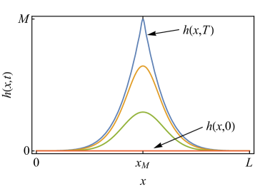
Figure 1: Situation considered in the present study: an initially flat profile $h(x,0)$ on a domain $0\leq x\leq L$ reaches a given maximum height $M$ for the first time at time $T$. $x_{M}$ denotes the location of this first-passage event. While the actual first-passage dynamics of the interface is stochastic [see Eqs. 1 and 2], we focus here on the weak-noise approximation as governed by the (non-stochastic) partial differential equations in Eqs. 14 and 44.

Interfacial fluctuations typically exhibit long-ranged correlations and non-Markovian dynamics. Roughening of interfaces and the associated dynamic scaling behavior emerging from Eqs. 1 and 2 has been extensively studied (see, e.g., Refs. Abraham and Upton (1989); Racz et al. (1991); Antal and Racz (1996); Barabasi and Stanley (1995); Majaniemi et al. (1996); Flekkoy and Rothman (1995, 1996); Krug (1997); Taloni et al. (2012); Gross and Varnik (2013); Halpin-Healy and Zhang (1995); Pruessner (2004); Cheang and Pruessner (2011)). More recently, extreme events and first-passage properties of interfaces have been investigated Krug et al. (1997); Majumdar and Bray (2001); Majumdar and Comtet (2004, 2005); Majumdar and Dasgupta (2006); Schehr and Majumdar (2006); Rambeau and Schehr (2010); Bray et al. (2013); Meerson and Vilenkin (2016); Meerson et al. (2016). The present study focuses on the time-evolution of a profile $h(x,t)$ governed by Eq. 1 or (2), under the condition that $h$ reaches a given height $M$ for the first time at time $T$,

$$h(x_{M},T)=M,$$ (4)

given that, initially,

$$h(x,t=0)=0.$$ (5)

The location $x_{M}$ where the height $M$ is reached first depends on the specific model as well as on the boundary conditions. If $T$ is larger than the relaxation time of the interface, the interfacial roughness (i.e., the one-point one-time variance of the height fluctuations) has saturated at the first-passage event Rowlinson and Widom (1982); Barabasi and Stanley (1995); Krug (1997) and the interface is accordingly governed by equilibrium dynamics (the precise meaning of this will be clarified further below). We consider profiles on a finite domain $[0,L]$ subject to either periodic boundary conditions (p),

$$h^{\text{(p)}}(x,t)=h^{\text{(p)}}(x+L,t),$$ (6)

or Dirichlet boundary conditions (D),

$$h^{\text{(D)}}(0,t)=0=h^{\text{(D)}}(L,t).$$ (7)

For the MH equation with Dirichlet boundary conditions, two further conditions are needed to completely determine the solution. We impose in this case a no-flux boundary condition (see also Appendix B):

$$\partial_{x}^{3}h^{(\mathrm{D}^{\prime})}(0,t)=0=\partial_{x}^{3}h^{(\mathrm{D}^{\prime})}(L,t),$$ (8)

and henceforth indicate Eqs. 7 and 8 by a superscript $\mathrm{(D^{\prime})}$ . We denote by the “mass” $\mathcal{A}$ the total area under the profile:

$$\mathcal{A}([h],t)\equiv\int_{0}^{L}\mathrm{d}x\,h(x,t).$$ (9)

For the EW equation with periodic boundary conditions, $\mathcal{A}([h^{\text{(p)}}],t)$ is not constant in time, but instead behaves diffusively at large times Krug (1997). In this case, we consider instead of $h^{\text{(p)}}$ the relative height fluctuation

$$\tilde{h}^{\text{(p)}}(x,t)\equiv h^{\text{(p)}}(x,t)-\mathcal{A}([h^{\text{(p)}}],t)/L\,,$$ (10)

which fulfills $\mathcal{A}([\tilde{h}^{\text{(p)}}],t)=0$. We henceforth drop the tilde on $\tilde{h}^{\text{(p)}}$ in order to simplify notation. Global conservation of the mass with

$$\mathcal{A}([h],t)=0$$ (11)

holds also for the MH equation with either periodic or Dirichlet no-flux boundary conditions [given Eq. 5]. For the EW equation with standard Dirichlet boundary conditions , the mass vanishes only after averaging over time. Equation 10, which is rather artificial from a physical point of view, is imposed here mainly in order to compare the different models under the common mass constraint, Eq. 11. The basic situation and the relevant quantities considered in the present study are illustrated in Fig. 1. In passing, we introduce the dynamic index $z$, which describes the dependence of the relaxation time $\tau$ of a typical fluctuation governed by Eq. (1) or (2) on the system size $L$ via $\tau\propto L^{z}$, with

$$z=2\qquad\text{(EW equation)},\qquad\qquad z=4\qquad\text{(MH equation)}.$$ (12)

Large deviations of stochastic processes are formally described by Freidlin-Wentzel theory Freidlin and Wentzell (1998); E et al. (2004); Luchinsky et al. (1998), which is equivalent to a Martin-Siggia-Rose/Janssen/de Dominicis path-integral formulation Martin et al. (1973); Janssen (1976); de Dominicis (1976); Täuber (2014) in the limit of weak noise Fogedby and Ren (2009); Ge and Qian (2012); Grafke et al. (2015). This approach provides an action functional, the minimization of which yields the most probable (“optimal”) path connecting two states [e.g., Eqs. (5) and (4)]. For an explicit derivation of the corresponding weak-noise theory (WNT) for the EW and MH equation see, e.g., Refs. Meerson and Vilenkin (2016); Smith et al. (2017). A related large deviation formalism in the context of lattice gases is reviewed in Ref. Bertini et al. (2015).

An important predecessor to the present work is Ref. Meerson and Vilenkin (2016), where the WNT of Eq. 2 with periodic boundary conditions has been solved. Here, we extend that study by discussing further aspects of the first-passage dynamics, focusing, in particular, on the effect of boundary conditions. Within the WNT of Eqs. 1 and 2, we obtain minimum-action paths describing extremal fluctuations of the profile fulfilling Eqs. 5 and 4, without conditioning on the first-passage. We remark that the solution of WNT for Dirichlet no-flux boundary conditions [Eqs. 7 and 8] is technically involved since it requires the consideration of an adjoint eigenproblem [see Sec. B.1.1]. Predictions of WNT will be compared to Langevin simulations in an accompanying paper Gross (2017).

The first-passage problem for the MH equation discussed here and in Ref. Gross (2017) is relevant, inter alia, for the rupture of liquid wetting films. In contrast to previous studies Bausch and Blossey (1994); Bausch et al. (1994); Blossey (1995); Foltin et al. (1997); Seemann et al. (2001); Thiele et al. (2001, 2002); Tsui et al. (2003); Becker et al. (2003); Gruen et al. (2006); Fetzer et al. (2007); Croll and Dalnoki-Veress (2010); Blossey (2012); Nguyen et al. (2014); Duran-Olivencia et al. (2017), we focus here on the case where disjoining pressure is negligible and film rupture is solely driven by noise. A related WNT describing the noise-induced breakup of a liquid thread has been analyzed in Ref. Eggers (2002). Rare-event trajectories of the kind considered here are furthermore relevant for the understanding of chemical reaction pathways E and Vanden-Eijnden (2010); Kim and Netz (2015); Delarue et al. (2017), phase transitions E et al. (2004); Li et al. (2012) as well as for certain aspects in interfacial wetting (see Ref. Belardinelli et al. (2016) and references therein).

The main results of the present study are contained in Secs. II and III, in which the necessary formalism of WNT for the EW and MH equation, respectively, is introduced and the exact analytical solution for the first-passage profile is discussed. The determination of the analytical solution as well as further mathematical details are deferred to Appendices A to C. In the main part (Secs. II.2 and III.2), we focus on the time-evolution of the first-passage profile in the case of periodic and Dirichlet (no-flux) boundary conditions. For first-passage times $T\ll\tau$ (transient regime) we find that the profile shape essentially depends only on the type of bulk dynamics, while the influence of boundary conditions and mass conservation is negligible. In contrast, at late times $T\gg\tau$ (equilibrium regime), the profile evolves over the whole domain and strongly depends on the specific boundary conditions. In both temporal regimes, simple analytical expressions for the asymptotic dynamic and static scaling profiles are derived. These scaling forms indicate that, within WNT, the peak height $h(x_{M},t)$ of the profile approaches the first-passage height $M$ in time with a universal exponent $1/z$. Moreover, it is shown that, in the presence of a microscopic cutoff, the dynamic scaling exponent eventually crosses over to a value of 1 close to the first-passage event.

II Edwards-Wilkinson equation

II.1 Macroscopic fluctuation theory

The Martin-Siggia-Rose field-theoretical action pertaining to Eq. 1 is given by Täuber (2014); Smith et al. (2017)

$$\mathcal{S}[h,p]=\int_{0}^{T}\mathrm{d}t\int_{0}^{L}\mathrm{d}x\,\left[p(\partial_{t}h-\eta\partial_{x}^{2}h)-Dp^{2}\right],$$ (13)

where $p$ is an auxiliary (“conjugate”) field. The most-probable (optimal) path emerging from the stochastic dynamics is the one that minimizes $\mathcal{S}$:

$$0 =\frac{\delta\mathcal{S}}{\delta p}=\partial_{t}h-\eta\partial_{x}^{2}h-2Dp,$$ (14a)

$$0 =\frac{\delta\mathcal{S}}{\delta h}=-\partial_{t}p-\eta\partial_{x}^{2}p\,.$$ (14b)

The field $p$, which can be interpreted as the typical noise magnitude, is governed by an anti-diffusion equation [Eq. 14b]. This indicates that the creation of a rare event requires the local accumulation of noise intensity. We consider either periodic boundary conditions [Eq. 6],

$$h^{\text{(p)}}(x,t)=h^{\text{(p)}}(x+L,t),\qquad p^{\text{(p)}}(x,t)=p^{\text{(p)}}(x+L,t),$$ (15)

or Dirichlet boundary conditions [Eq. 7],

$$h^{\text{(D)}}(0,t)=0=h^{\text{(D)}}(L,t),\qquad p^{\text{(D)}}(0,t)=0=p^{\text{(D)}}(L,t).$$ (16)

Note that, since $\partial_{x}^{2}$ is self-adjoint on $[0,L]$ for the considered boundary conditions, $p$ fulfills the same boundary conditions as $h$ (see also Appendices B and C). Inserting the mean-field equations (14) into the action in Eq. 13 yields the optimal action

$$\mathcal{S}_{\text{opt}}=D\int_{0}^{T}\mathrm{d}t\int_{0}^{L}\mathrm{d}x\,p^{2}.$$ (17)

Equation 14 admits a special solution which can be identified with thermal equilibrium. In equilibrium, the most-likely noise-activated trajectory $h(x,t)$ is the time-reversed of the corresponding relaxation trajectory $h_{r}(x,t)$ — a property known as Onsager-Machlup symmetry Onsager and Machlup (1953). In order to exhibit this symmetry for the dynamics described by Eq. 14, consider the solution $h_{r}(x,t)$ of the noise-free analog of Eq. 14a, i.e., the diffusion equation

$$\partial_{t}h_{r}=\eta\partial_{x}^{2}h_{r},$$ (18)

with initial condition $h_{r}(x,t=0)=h_{0}(x)$, where $h_{0}(x)$ is a given profile [e.g. the equilibrium first-passage profile $h(x,T\to\infty)$, which can be determined independently, see Eq. 35 below]. Then, the solution $h(x,t)$, $p(x,t)$ of Eq. 14, fulfilling $h(x,T)=h_{0}(x)$ at some final time $T$, is given by

$$h(x,t)=h_{r}(T-t),\quad p(x,t)=-\frac{\eta}{D}\partial_{x}^{2}h(x,t).$$ (19)

Indeed, it is readily checked that Eq. 19 solves Eq. 14, as

$$\partial_{t}h=-\partial_{t}h_{r}=-\eta\partial_{x}^{2}h=\eta\partial_{x}^{2}h+2Dp,$$ (20)

which is precisely Eq. 14a; furthermore $\partial_{t}p=-(\eta/D)\partial_{x}^{2}\partial_{t}h=(\eta^{2}/D)\partial_{x}^{4}h=-\eta\partial_{x}^{2}p$, which is Eq. 14b. According to Eq. 20, $h$ effectively obeys an anti-diffusion equation in the equilibrium regime. Note that the ansatz in Eq. 19 implies that the time evolution starts at time $t=0$ from the initial configuration $h(x,0)=h_{r}(T)$, which is flat only for $T\to\infty$. Accordingly, under requirement of Eq. 5, the equilibrium regime corresponds to large first-passage times $T$—as anticipated in Sec. I. The general solution of Eq. 14 fulfilling Eqs. 5 and 4 for arbitrary $T$ is presented below.

In the equilibrium regime, upon using Eqs. 19 and 20, the optimal action in Eq. 17 reduces to

$$\begin{split}\mathcal{S}_{\text{opt,eq}}&=\frac{\eta^{2}}{D}\int_{0}^{T}\mathrm{d}t\int_{0}^{L}\mathrm{d}x\,(\partial_{x}^{2}h)^{2}=-\frac{\eta^{2}}{D}\int_{0}^{T}\mathrm{d}t\int_{0}^{L}\mathrm{d}x\,(\partial_{x}h)(\partial_{x}^{3}h)\\ &=\frac{\eta}{D}\int_{0}^{T}\mathrm{d}t\int_{0}^{L}\mathrm{d}x\,(\partial_{x}h)(\partial^{2}_{xt}h)=\frac{\eta}{D}\int_{0}^{L}\mathrm{d}x\,(\partial_{x}h)^{2}\Big{|}_{0}^{T}-\frac{\eta}{D}\int_{0}^{T}\mathrm{d}t\int_{0}^{L}\mathrm{d}x\,(\partial^{2}_{xt}h)(\partial_{x}h)\\ &=\frac{\eta}{2D}\int_{0}^{L}\mathrm{d}x\,(\partial_{x}h)^{2}\Big{|}_{0}^{T}.\end{split}$$ (21)

In the partial integrations above we made use of the fact that the spatial boundary terms generally vanish for periodic and Dirichlet boundary conditions . Equation 21 provides a fluctuation-dissipation relation, from which the temperature $\Theta$ (in units of $k_{B}$) can be identified via $\eta/(2D)=1/(4\Theta)$.

We henceforth consider time to be rescaled by the friction coefficient $\eta$, i.e., $\tilde{t}=\eta t$, and define new fields $\tilde{h}$, $\tilde{p}$ via

$$h(x,t)\equiv\tilde{h}(x,\eta t),\qquad p(x,t)=(\eta/D)\tilde{p}(x,\eta t).$$ (22)

The Euler-Lagrange equations in Eq. 14 can then be cast into the form

$$\partial_{\tilde{t}}\tilde{h} =\partial_{x}^{2}\tilde{h}+2\tilde{p},$$ (23a)

$$\partial_{\tilde{t}}\tilde{p} =-\partial_{x}^{2}\tilde{p}\,.$$ (23b)

Analogously, $\mathcal{S}_{\text{opt}}$ in Eq. 17 can be expressed in terms of the rescaled action

$$\tilde{\mathcal{S}}_{\text{opt}}\equiv\int_{0}^{\tilde{T}}\mathrm{d}\tilde{t}\int_{0}^{L}\mathrm{d}x\,\tilde{p}(x,\tilde{t})^{2}$$ (24)

as

$$\mathcal{S}_{\text{opt}}=\frac{\eta}{D}\tilde{\mathcal{S}}_{\text{opt}},$$ (25)

with $\tilde{T}\equiv\eta T$. It is useful to remark that the dimension of $\eta/D$ is the same as of $L/M^{2}$. Equation 25 makes it obvious that the saddle-point solution of the action dominates the dynamics in the weak-noise limit $D\to 0$. We proceed with the analysis of Eqs. 23 and 24 and henceforth drop the tilde in order to simplify the notation.

II.2 Exact solution

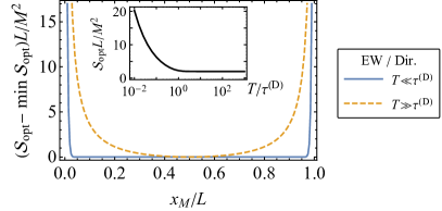
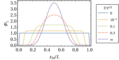
Figure 2: (a) Optimal action $\mathcal{S}_{\text{opt}}^{\text{(D)}}$ [Eq. 27] for the EW equation with Dirichlet boundary conditions. The curves for $\mathcal{S}_{\text{opt}}^{\text{(D)}}$ are shifted such that their respective minima are zero. For sufficiently large or small $T$, $\mathcal{S}_{\text{opt}}^{\text{(D)}}-\mathrm{min}\mathcal{S}_{\text{opt}}^{\text{(D)}}$ becomes independent of $T$. Asymptotically for $T\to 0$ in the transient regime, $\mathcal{S}_{\text{opt}}^{\text{(D)}}$ is spatially constant (and nonzero) for $0<x_{M}<L$. Due to Dirichlet boundary conditions, $\mathcal{S}_{\text{opt}}^{\text{(D)}}$ diverges for $x_{M}=0,L$. The inset shows $\mathcal{S}_{\text{opt}}^{\text{(D)}}$ evaluated for $x_{M}=L/2$, which approaches a nonzero constant for $T\gg\tau^{\text{(D)}}$ and diverges $\propto T^{-1/z}$ as $T\to 0$ [see Eq. 183]. (b) Probability distribution $\mathcal{P}_{1}^{\text{(D)}}$ [Eq. 28] of the first-passage location $x_{M}$ for Dirichlet boundary conditions, $M^{2}/L=2$ (in units of $\eta/D$) and various values of $T/\tau^{\text{(D)}}$. The curves labeled by $T/\tau^{\text{(D)}}=0$ and $\infty$ pertain to the asymptotic transient and the equilibrium regime, respectively, where $\mathcal{P}_{1}^{\text{(D)}}$ is independent of $T$. Upon increasing $M^{2}/L$, the width of the curves (except the one corresponding to $T/\tau^{\text{(D)}}\to 0$) decrease and their peak height increases.

The solution of Eq. 23 subject to the initial and final conditions in Eqs. 4 and 5 as well as to the boundary conditions in Eq. 15 or Eq. 16 can be determined exactly [see Appendix C] and is summarized below. It turns out that initial and final conditions for $p$ do not have to be specified additionally, but instead implicitly follow from the ones imposed on $h$. Two characteristic regimes can be distinguished: a transient regime, corresponding to first-passage times $T\ll\tau$, and an equilibrium regime, corresponding to $T\gg\tau$. The relaxation time $\tau$ is given by ($z=2$)

$$\tau^{\text{(p)}} =\left(\frac{L}{2\pi}\right)^{z}$$ (26a)

for periodic and by

$$\tau^{\text{(D)}} =\left(\frac{L}{\pi}\right)^{z}$$ (26b)

for Dirichlet boundary conditions. Within WNT, $\tau$ is in fact the characteristic time scale for the creation of a first-passage event. Asymptotically for $T\to\infty$, the profile in the equilibrium regime fulfills Eq. 19.

The optimal action [Eq. 24] has the following formal scaling property [see Appendix C]:

$$\mathcal{S}_{\text{opt}}(x_{M},M,T,L)=\frac{M^{2}}{L}\mathcal{S}_{\text{opt}}\left(\frac{x_{M}}{L},1,\frac{T}{L^{z}},1\right).$$ (27)

Recalling Eq. 25, Eq. 27 accordingly demonstrates that, within WNT, the weak-noise limit $D\to 0$ is equivalent to the limit of large heights $M^{2}/L\to\infty$. Furthermore, $\mathcal{S}_{\text{opt}}$ determines the probability distribution of the first-passage coordinate $x_{M}$,

$$\mathcal{P}_{1}(x_{M})\sim\exp[-\mathcal{S}_{\text{opt}}(x_{M},M,T,L)],$$ (28)

which is assumed to be normalized such that $\int_{0}^{L}\mathrm{d}x_{M}\,\mathcal{P}_{1}(x_{M})=1$. For the purpose of numerical evaluation it is convenient to use the relation $\mathcal{S}_{\text{opt}}(x_{M},M,T,L)=M^{2}/[2Q(x_{M},T,L)]$, where the function $Q$ is reported in Eq. 155. Figure 2 displays $\mathcal{S}_{\text{opt}}^{\text{(D)}}$ as a function of $x_{M}$ for Dirichlet boundary conditions in the asymptotic transient ($T\ll\tau^{\text{(D)}}$) and equilibrium regimes ($T\gg\tau^{\text{(D)}}$). In equilibrium, $\mathcal{S}_{\text{opt}}$ generally simplifies to $\mathcal{S}_{\text{opt,eq}}$ in Eq. 21. Minimization of $\mathcal{S}_{\text{opt,eq}}^{\text{(D)}}$ yields [see Appendix A]

$$x_{M}^{(\mathrm{D})}=L/2.$$ (29)

Asymptotically for $T\to 0$ one has $\mathcal{S}_{\text{opt}}\propto T^{-1/z}$ [see Eq. 183]. Specifically, for $T\to 0$ and Dirichlet boundary conditions, $\mathcal{S}_{\text{opt}}^{\text{(D)}}$ becomes independent of $x_{M}$ for $0<x_{M}<L$ and diverges for $x_{M}\in\{0,L\}$. For definiteness, we shall henceforth take for $x_{M}$ in the transient regime the same value as in Eq. 29. In fact, since the short-time profile is strongly localized for $T\to 0$ [see, e.g., Fig. 5(a)], its shape is independent of the precise value of $x_{M}$. In Fig. 2, the first-passage distribution in Eq. 28 is illustrated for Dirichlet boundary conditions and an (arbitrarily chosen) reduced height $M^{2}/L=2$ [in units of $\eta/D$, see Eq. 25]. One observes a smooth transition between the shapes pertaining to the asymptotic transient and equilibrium regimes, in both of which $\mathcal{P}_{1}^{\text{(D)}}$ is independent of $T$. Upon increasing the value of $M^{2}/L$ for nonzero $T/\tau^{\text{(D)}}$, the maximum height of the distribution increases and, correspondingly, its width decreases. In the limit $M^{2}/L\to\infty$, $\mathcal{P}_{1}$ approaches a Dirac delta-function.

The profile $h(x,t)$ solving Eq. 23 can be brought into the following scaling form:

$$h(x,t,T,M,L)=M\mathpzc{h}\left(\frac{x}{L},\frac{t}{\tau},\frac{T}{\tau}\right),$$ (30)

where, for periodic boundary conditions, the scaling function $\mathpzc{h}$ is given by [see Eqs. 160 and 161]

$$\mathpzc{h}^{\text{(p)}}(\mathrm{x},\mathrm{t},\mathrm{T})=\frac{1}{\mathpzc{Q}^{\text{(p)}}(\mathrm{T})}\sum_{k=1}^{\infty}\frac{1-\exp\left(-2k^{2}\mathrm{T}\right)}{k^{2}}\frac{\sinh\left(k^{2}\mathrm{t}\right)}{\sinh\left(k^{2}\mathrm{T}\right)}\cos\left(2\pi k(\mathrm{x}-1/2)\right)$$ (31)

with

$$\mathpzc{Q}^{\text{(p)}}(\mathrm{T})\equiv\sum_{k=1}^{\infty}\frac{1-\exp\left(-2k^{2}\mathrm{T}\right)}{k^{2}}.$$ (32)

Although $\mathcal{S}_{\text{opt}}^{\text{(p)}}$ [Eq. 24] is manifestly independent of $x_{M}$ owing to translational invariance, for definiteness we choose $x_{M}^{\text{(p)}}=L/2$, which also simplifies the expressions for $h$ somewhat. As a consequence of explicitly enforcing the mass constraint [Eq. 11] in this case, the zero-mode ($k=0$) is absent from Eqs. 31 and 32 [see Eq. 158]. Indeed, since $\int_{0}^{L}\mathrm{d}x\,\cos(2\pi k(x/L-1/2))=0$ for $k\geq 1$, the mass vanishes identically for $h^{\text{(p)}}$. For Dirichlet boundary conditions, using Eq. 29, one has [see Eqs. 162, 163, 164 and 165]

$$\mathpzc{h}^{\text{(D)}}(\mathrm{x},\mathrm{t},\mathrm{T})=\frac{1}{\mathpzc{Q}^{\text{(D)}}(\mathrm{T})}\sum_{k=1,3,5,\ldots}^{\infty}\frac{1-\exp\left(-2k^{2}\mathrm{T}\right)}{k^{2}}\frac{\sinh\left(k^{2}\mathrm{t}\right)}{\sinh\left(k^{2}\mathrm{T}\right)}\cos\left(\pi k(\mathrm{x}-1/2)\right)$$ (33)

with

$$\mathpzc{Q}^{\text{(D)}}(\mathrm{T})\equiv\sum_{k=1,3,5,\ldots}^{\infty}\frac{1-\exp\left(-2k^{2}\mathrm{T}\right)}{\lambda_{k}^{2}}.$$ (34)

Since $x_{M}^{\text{(D)}}=L/2$, the above sums run only over the odd eigenmodes $k=1,3,5,\ldots$, which have nonzero mass, $\int_{0}^{L}\mathrm{d}x\,\sin(k\pi x/L)=L/(k\pi)$ (eigenfunctions for even $k$ have vanishing mass). The general expression for the conjugate field $p(x,t)$ is provided in Eq. 156.

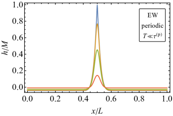
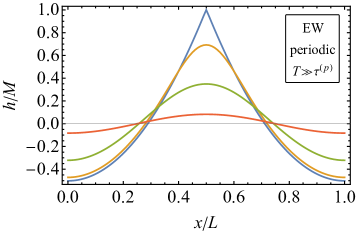
Figure 3: Time evolution of the optimal profile [Eqs. 30 and 31] for the EW equation with periodic boundary conditions in (a) the transient and (b) the equilibrium regime. The curves correspond, from center top to bottom, to (a) $1-t/T=0,0.1,0.4,0.8$ with $T=10^{-2}\tau^{\text{(p)}}$, and (b) $1-t/T=0,0.001,0.006,0.02$ with $T=100\tau^{\text{(p)}}$. Decreasing $T$ in (a) leads essentially to a reduction of the width of the curves [see also Eq. 40]. The fundamental time scale $\tau^{\text{(p)}}$ is reported in Eq. 26a.

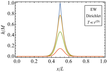
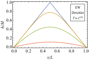
Figure 4: Time evolution of the optimal profile [Eqs. 30 and 33] for the EW equation with Dirichlet boundary conditions in (a) the transient and (b) the equilibrium regime. The curves correspond, from center top to bottom, to (a) $1-t/T=0,0.1,0.4,0.8$ with $T=10^{-2}\tau^{\text{(D)}}$, and (b) $1-t/T=0,0.001,0.006,0.02$ with $T=100\tau^{\text{(D)}}$. Decreasing $T$ in (a) leads essentially to a reduction of the width of the curves [see also Eq. 40]. The fundamental time scale $\tau^{\text{(D)}}$ is reported in Eq. 26b.

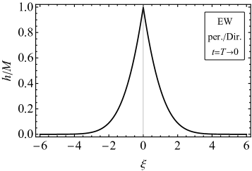
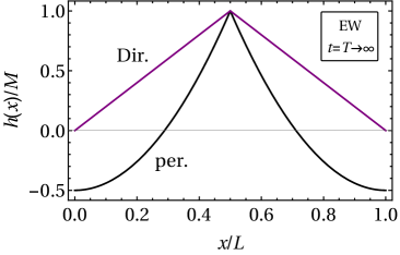
Figure 5: Asymptotic first-passage profiles $h(x,t=T)$ (normalized by $M$) obtained within WNT of the EW equation [Eq. 1] in (a) the transient regime, $T\to 0$ [Eq. 38], and (b) the equilibrium regime, $T\to\infty$ [Eq. 35]. In the transient regime, the profiles depend on the scaling variable $\xi\equiv(x-L/2)/(2T)^{1/2}$ and are identical for periodic and Dirichlet boundary conditions. In the equilibrium regime, the (normalized) profile is a function of $x/L$ and is specific to each boundary condition.

The typical spatio-temporal evolution of $h(x,t)$ is illustrated in Figs. 3 and 4 for periodic and Dirichlet boundary conditions, respectively. In the equilibrium regime ($T\gg\tau$), the profile at time $t=T\to\infty$ can be readily calculated from Eqs. 31 and 33 [see Eq. 194 in Sec. C.2.2]:

$$h^{\text{(p)}}(x,T)\big{|}_{T\to\infty}/M =1-6\Bigg{|}\frac{x}{L}-\frac{1}{2}\Bigg{|}+6\left(\frac{x}{L}-\frac{1}{2}\right)^{2},$$ (35a)

$$h^{\text{(D)}}(x,T)\big{|}_{T\to\infty}/M =1-\left|1-\frac{2x}{L}\right|.$$ (35b)

The same results are obtained via minimization of the equilibrium action in Eq. 21, using the fact that $h(x,0)=0$ [see Appendix A]. For times $t=T-\delta t<T$ with $\delta t\ll T$ and $T\gg\tau$, Eq. 30 adopts a reduced dynamic scaling form [see Eq. 200]:

$$h(x,T-\delta t)\big{|}_{T\gg\tau}\simeq M-M(\delta t)^{1/z}\Gamma(1-1/z)\tilde{\mathcal{H}}\left(\frac{x-L/2}{\delta t^{1/z}}\right),\qquad z=2,$$ (36)

with the scaling function

$$\tilde{\mathcal{H}}(\xi)=\exp\left(-\frac{\xi^{2}}{4}\right)+\frac{1}{2}\sqrt{\pi}\,\xi\,\mathrm{erf}\left(\frac{\xi}{2}\right),$$ (37)

both for periodic and Dirichlet boundary conditions. It is convenient to carry along the dynamic index $z$ [Eq. 12] in these and the following expressions. Note that $\eta$ has the same dimension as $L^{z}/T$, such that, upon re-instating the unscaled quantities [see Eq. 22], the argument of $\tilde{\mathcal{H}}$ in Eq. 36 is seen to be dimensionless.

In the transient regime ($T\ll\tau$), the scaling profile at time $t=T$ is given by [see Eq. 180]:

$$h(x,T)\big{|}_{T\ll\tau}=M\mathcal{H}\left(\frac{x-L/2}{(2T)^{1/z}}\right),\qquad z=2,$$ (38)

with the scaling function

$$\mathcal{H}(\xi)=\exp\left(-\frac{\xi^{2}}{4}\right)+\frac{1}{2}\sqrt{\pi}|\xi|\left[\mathrm{erf}\left(\frac{|\xi|}{2}\right)-1\right].$$ (39)

Since there is no risk of confusion, we use the same symbol $\xi$ for the scaling variables in Eqs. 37 and 39. For times $t=T-\delta t<T$ in the limit $\delta t/T\to 0$ (with $T\ll\tau$), a dynamic scaling profile follows as [see Eq. 187]

$$h(x,T-\delta t)\Big{|}_{\begin{subarray}{c}T\ll\tau\\ \delta t\ll T\end{subarray}}=M-M\left(\frac{\delta t}{2T}\right)^{1/z}\tilde{\mathcal{H}}\left(\frac{x-L/2}{\delta t^{1/z}}\right),\qquad z=2,$$ (40)

with the same scaling function as in Eq. 37. The above scaling profiles are independent of the specific boundary condition and apply for values of the scaling variable $|\xi|\lesssim\mathcal{O}(1)$, i.e. in an “inner” region near the first-passage location $x_{M}$. The accuracy of the approximations involved in Eq. 40 is further illustrated in Fig. 14 in Appendix C. [A short-time scaling profile for finite nonzero $\delta t\ll T$, which entails a scaling function different from $\tilde{\mathcal{H}}$, is provided in Eq. 185.] Note that the final profile in the transient regime [Eq. 38] still depends on $T$ via the scaling variable $\xi$, whereas the final profile in the equilibrium regime [Eq. 35] is independent of $T$ for $T\gg\tau$. We remark that, in contrast to the exact expression in Eq. 31, $h^{\text{(p)}}$ as given in Eq. 38 has nonzero mass. This, however, constitutes a negligible error in the asymptotic limit $T\to 0$, as the profile becomes sharply peaked. The final profiles in the transient and the equilibrium regime are illustrated in Fig. 5.

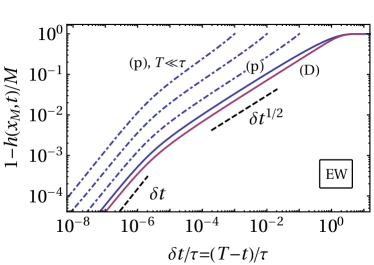
Figure 6: Time evolution of the peak of the profile, $h(x_{M},t)$, which reaches the height $M$ at the first-passage time $T$, for the EW equation as a function of $T-t$. The solid curves correspond to $h^{\text{(p,D)}}(x_{M},t)$ in the equilibrium regime, while the dash-dotted curves illustrate the time evolution of $h^{\text{(p)}}(x_{M},t)$ in the transient regime for $T/\tau=10^{-1},10^{-2},10^{-3}$ (from bottom to top). The corresponding behavior of $h^{(\mathrm{D})}(x_{M},t)$ for $t\ll T$ is similar and not shown. Both in the transient and the equilibrium regime, a power law $M-h(x_{M},T-\delta t)\propto\delta t^{1/2}$ is predicted [see Eq. 41]. In the presence of an upper bound to the number of (eigen-)modes in the system, a linear behavior in $\delta t$ emerges for times $\delta t\lesssim\tau_{\times}=\tau/k_{\times}^{z}$ [see Eq. 42], where $k_{\times}$ is the largest mode index ($k_{\times}=\infty$ in the continuum limit). For illustrative purposes, we have chosen here $k_{\times}=1000$, corresponding to $\tau_{\times}/\tau\simeq 10^{-6}$. The fundamental time scale $\tau$ is defined in Eq. 26 for the respective boundary conditions.

According to Eqs. 36 and 40 the maximum $h(x_{M},t)$ of the profile approaches the height $M$ at the first-passage time $T$ via a power law,

$$1-h(x_{M},T-\delta t)/M\propto\delta t^{1/z},\qquad z=2.$$ (41)

This behavior applies both in the transient and the equilibrium regime and is independent of the boundary conditions. If the system considered can accommodate only a finite number of modes—which, for instance, is the case when Eqs. 1 and 2 are discretized on a lattice—the sums in Eqs. 31 to 34 are bounded by a largest mode $k_{\times}$. In this case, Eq. 41 is eventually superseded by a linear behavior,

$$1-h(x_{M},T-\delta t)/M\propto\delta t\qquad\text{for}\qquad\delta t\lesssim\tau_{\times}\equiv\tau/k_{\times}^{z},$$ (42)

where $\tau_{\times}$ denotes the corresponding cross-over time [see Eq. 202]. The time evolution of the peak $h(x_{M},t)$ is illustrated in Fig. 6, where the time is rescaled by the characteristic relaxation time $\tau$ in Eq. 26. Note that, in the equilibrium regime, the evolution of the profile towards the first-passage event happens on a time scale of $\tau$, independently from the value of $T$. For times $t\ll T-\tau$ the equilibrium profile thus remains near its initial configuration [Eq. 5; see also panels (b) in Figs. 3 and 4]. In the transient regime [dash-dotted lines in Fig. 6 and panels (a) in Figs. 3 and 4], the evolution proceeds over the whole time interval between 0 and $T$ (where, however, $T\ll\tau$).

According to Eq. 41, the distance $M$ is traversed within a time $\delta t^{1/z}$. Consequently, the requirement $\delta t\ll\tau$ for the transient regime implies $M/L\ll 1/(c\pi)$, with $c^{\text{(p)}}=2$ and $c^{(\mathrm{D})}=1$ [see Eq. 26]. Hence, in the transient regime, the weak-noise limit of Eq. 27 is obtained if $L\gg\frac{D}{\eta}\left(\frac{L}{M}\right)^{2}\gg\frac{D}{\eta}(c\pi)^{2}$, where we re-instated all dimensional factors. Conversely, the equilibrium regime is realized if $M/L\gg 1/(c\pi)$, such that in this case the weak-noise limit requires $L\gg\frac{D}{\eta}\left(\frac{L}{M}\right)^{2}$ and $\left(\frac{L}{M}\right)^{2}\ll(c\pi)^{2}$.

III Mullins-Herring dynamics

We now turn to the optimal first-passage dynamics emerging from the MH equation. The analysis in this section proceeds in essentially the same fashion as for the EW equation in Sec. II. However, at the expense of some redundancy, the subsequent discussion is kept largely self-contained.

III.1 Macroscopic fluctuation theory

The Martin-Siggia-Rose action pertaining to the stochastic MH equation [Eq. 2] is given by Täuber (2014)

$$\mathcal{S}[h,p]=\int_{0}^{T}\mathrm{d}t\int_{0}^{L}\mathrm{d}x\,p\left[\partial_{t}h+\eta\partial_{x}^{4}h+D\partial_{x}^{2}p\right].$$ (43)

The Euler-Lagrange equations describing the most-likely path of the profile $h$ and of the conjugate field $p$ follow as (see also Ref. Smith et al. (2017))

$$0 =\frac{\delta\mathcal{S}}{\delta p}=\partial_{t}h+\eta\partial_{x}^{4}h+2D\partial_{x}^{2}p,$$ (44a)

$$0 =\frac{\delta\mathcal{S}}{\delta h}=-\partial_{t}p+\eta\partial_{x}^{4}p.$$ (44b)

We consider either periodic boundary conditions [Eq. 6],

$$h^{\text{(p)}}(x,t)=h^{\text{(p)}}(x+L,t),\qquad p^{\text{(p)}}(x,t)=p^{\text{(p)}}(x+L,t),$$ (45)

or Dirichlet boundary conditions with a no-flux condition [Eqs. 7 and 8],

$$h^{(\mathrm{D}^{\prime})}(0,t)=0=h^{(\mathrm{D}^{\prime})}(L,t),\qquad\partial_{x}^{3}h^{(\mathrm{D}^{\prime})}(0,t)=0=\partial_{x}^{3}h^{(\mathrm{D}^{\prime})}(L,t).$$ (46)

In the latter case, the bi-harmonic operator $\partial_{x}^{4}$ is not self-adjoint on $[0,L]$, which renders the solution of Eq. 44 technically more involved than in the self-adjoint case (see Appendix C). If Dirichlet no-flux boundary conditions are imposed on $h$, the conjugate field $p$ must fulfill the associated adjoint boundary conditions (see Appendix B)

$$\partial_{x}p^{(\mathrm{D}^{\prime})}(0,t)=0=\partial_{x}p^{(\mathrm{D}^{\prime})}(L,t),\qquad\partial_{x}^{2}p^{(\mathrm{D}^{\prime})}(0,t)=0=\partial_{x}^{2}p^{(\mathrm{D}^{\prime})}(L,t).$$ (47)

The mass-conserving property of the noise in Eq. 2 is reflected by the presence of a derivative of $p$ in Eq. 44a. Indeed, it is readily proven that the considered boundary conditions ensure conservation of the mass [Eq. 11]. Initial and final conditions on the profile $h$ are given in Eqs. 5 and 4 and suffice to determine also the conjugate field $p$. Inserting Eq. 44 into Eq. 43 renders the optimal action

$$\mathcal{S}_{\text{opt}}=-D\int_{0}^{T}\mathrm{d}t\int_{0}^{L}\mathrm{d}x\,p\partial_{x}^{2}p,$$ (48)

which describes the most-likely activation dynamics Meerson and Vilenkin (2016); Smith et al. (2017).

As was the case for the EW equation (see Sec. II.1), Eq. 44 admits, as a manifestation of the Onsager-Machlup time-reversal symmetry Onsager and Machlup (1953), a specific solution corresponding to thermal equilibrium. In fact, consider a profile $h_{r}(x,t)$ obeying the (deterministic) fourth-order diffusion equation

$$\partial_{t}h_{r}=-\eta\partial_{x}^{4}h_{r},$$ (49)

with the initial condition $h_{r}(x,t=0)=h_{0}(x)$, where $h_{0}(x)$ is a given profile [e.g., $h_{0}(x)=h(x,T\to\infty)$, where $h(x,T\to\infty)$ is a known first-passage profile]. Then the fields $h$, $p$ defined by

$$h(x,t) =h_{r}(x,T-t)\qquad\text{and}$$ (50a)

$$p(x,t) =-\frac{\eta}{D}\partial_{x}^{2}h$$ (50b)

fulfill the relations

$$\partial_{t}h=-\partial_{t}h_{r}=\eta\partial_{x}^{4}h=-\eta\partial_{x}^{4}h-2D\partial_{x}^{2}h$$ (51)

as well as $\partial_{t}p=-(\eta/D)\partial_{t}\partial_{x}^{2}h=-(\eta^{2}/D)\partial_{x}^{6}h_{r}=\eta\partial_{x}^{4}p$, which coincide with Eqs. 44a and 44b, respectively. Accordingly, the fields defined in Eq. 50 solve Eq. 44 subject to the final condition $h(x,T)=h_{0}(x)$. Equation 50a implies that $h(x,t=0)=h_{r}(x,T)$, which is generally nonzero for non-vanishing $h_{0}(x)$ and finite $T$. Hence, only for $T\to\infty$, equilibrium dynamics is strictly compatible with the initial condition in Eq. 5. Using Eqs. 50 and 51 in Eq. 48 renders the equilibrium action:

$$\begin{split}\mathcal{S}_{\text{opt,eq}}&=-\frac{\eta^{2}}{D}\int_{0}^{T}\mathrm{d}t\int_{0}^{L}\mathrm{d}x(\partial_{x}^{2}h)(\partial_{x}^{4}h)=\int_{0}^{T}\mathrm{d}t\left[-\frac{\eta}{D}(\partial_{x}h)(\partial_{t}h)\Big{|}_{0}^{L}+\frac{\eta^{2}}{D}\int_{0}^{L}\mathrm{d}x(\partial_{x}h)(\partial_{x}^{5}h)\right]\\ &=-\frac{\eta}{D}\left[h(\partial_{x}h)\Big{|}_{0}^{L}\right]_{t=0}^{T}+\frac{\eta}{D}\int_{0}^{T}\mathrm{d}t\,h(\partial_{tx}^{2}h)\Big{|}_{0}^{L}+\frac{\eta}{D}\int_{0}^{T}\mathrm{d}t\int_{0}^{L}\mathrm{d}x(\partial_{x}h)(\partial_{tx}^{2}h)\\ &=\frac{\eta}{D}\left[\int_{0}^{L}\mathrm{d}x(\partial_{x}h)^{2}\Bigg{|}_{t=0}^{T}-\int_{0}^{T}\mathrm{d}t\int_{0}^{L}\mathrm{d}x(\partial_{tx}^{2}h)(\partial_{x}h)\right]\\ &=\frac{\eta}{2D}\int_{0}^{L}\mathrm{d}x(\partial_{x}h)^{2}\Bigg{|}_{t=0}^{T},\end{split}$$ (52)

where we made use of the fact that the boundary terms vanish for the boundary conditions in Eqs. 45 and 46. In Eq. 52 the temperature $\Theta$ can be identified via $\eta/(2D)=1/(4\Theta)$. As expected, the final expression in Eq. 52 coincides with the one in Eq. 21 and shows that, in thermal equilibrium, the action essentially reduces to a free energy difference.

Upon rescaling time by $\eta$ and redefining the fields $h$ and $p$ as in Eq. 22, Eq. 44 becomes

$$\partial_{t}h =-\partial_{x}^{4}h-2\partial_{x}^{2}p,$$ (53a)

$$\partial_{t}p =\partial_{x}^{4}p.$$ (53b)

We henceforth consider also $\mathcal{S}_{\text{opt}}$ to be rescaled as in Eq. 25 and proceed by analyzing Eq. 53.

III.2 Exact solution

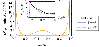
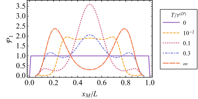
Figure 7: (a) Optimal action $\mathcal{S}_{\text{opt}}^{(\mathrm{D}^{\prime})}$ [Eq. 55, in units of $\eta/D$] for the MH equation with Dirichlet no-flux boundary conditions. The curves representing $\mathcal{S}_{\text{opt}}^{(\mathrm{D}^{\prime})}$ are shifted such that their respective minima are zero. For sufficiently large or small $T$, $\mathcal{S}_{\text{opt}}^{(\mathrm{D}^{\prime})}-\mathrm{min}\mathcal{S}_{\text{opt}}^{(\mathrm{D}^{\prime})}$ becomes independent of $T$. Asymptotically for $T\to 0$, $\mathcal{S}_{\text{opt}}^{(\mathrm{D}^{\prime})}$ is spatially constant for $0<x_{M}<L$ and diverges at the boundaries. The inset shows $\mathcal{S}_{\text{opt}}^{(\mathrm{D}^{\prime})}(x_{M}=x_{M}^{(\mathrm{D}^{\prime})})$ (solid curve) and $\mathcal{S}_{\text{opt}}^{(\mathrm{D}^{\prime})}(x_{M}=L/2)$ (dash-dotted curve) as functions of $T$. These quantities diverge $\propto T^{-1/z}$ as $T\to 0$ [see Eq. 183] and attain a nonzero constant for $T\gg\tau^{(\mathrm{D}^{\prime})}$. (b) Probability distribution $\mathcal{P}_{1}^{(\mathrm{D}^{\prime})}$ [Eq. 56] of the first-passage location $x_{M}$ for Dirichlet no-flux boundary conditions with $M^{2}/L=1$ (in units of $\eta/D$) and various values of $T$. The curves labeled by $T/\tau^{(\mathrm{D}^{\prime})}=0$ and $\infty$ represent the asymptotic shapes in the transient and the equilibrium regime, respectively, where $\mathcal{P}_{1}$ is independent of $T$.

The exact analytic solution of Eq. 53 subject to the the initial and final conditions in Eqs. 5 and 4 as well as to the boundary conditions in Eq. 45 or Eq. 46 is determined in detail in Appendix C and summarized below. The characteristic time scale for the creation of a rare event is given by ($z=4$)

$$\tau^{\text{(p)}} =\left(\frac{L}{2\pi}\right)^{z}$$ (54a)

for periodic and by

$$\tau^{(\mathrm{D}^{\prime})} =\left(\frac{L}{\omega_{1}}\right)^{z}$$ (54b)

for Dirichlet no-flux boundary conditions, respectively, where $\omega_{1}\simeq 4.73$ is the smallest positive solution of the eigenvalue equation $\cos(\omega)\cosh(\omega)=1$ [see Eq. 104]. As was the case for the EW equation, the dynamics emerging from Eq. 53 is distinct in the transient ($T\ll\tau$) and the equilibrium ($T\gg\tau$) regime. In the latter case, Eq. 50 applies.

Analogously to Eq. 27, the optimal action [see Eqs. 48 and 157; expressed in units of $\eta/D$] fulfills the formal scaling property

$$\mathcal{S}_{\text{opt}}(x_{M},M,T,L)=\frac{M^{2}}{L}\mathcal{S}_{\text{opt}}\left(\frac{x_{M}}{L},1,\frac{T}{L^{z}},1\right).$$ (55)

The value of the first-passage location $x_{M}$ [see Eq. 4] follows from minimizing $\mathcal{S}_{\text{opt}}$ evaluated on the general solution in Eq. 53. For periodic boundary conditions, one may simply set $x_{M}^{\text{(p)}}=L/2$ owing to translational invariance. For Dirichlet no-flux boundary conditions, the optimal action $\mathcal{S}_{\text{opt}}^{(\mathrm{D}^{\prime})}$ is shown as a function of $x_{M}$ in Fig. 7(a). Figure 7(b) displays the corresponding (normalized) probability distribution of the first-passage location $x_{M}$,

$$\mathcal{P}_{1}(x_{M})\sim\exp\left[-\mathcal{S}_{\text{opt}}(x_{M},M,T,L)\right].$$ (56)

For illustrative purposes, we have chosen $M^{2}/L=1$ (in units of $\eta/D$) in the plot, and remark that, upon increasing $M^{2}/L$, the peak height of the distribution grows and, correspondingly, its characteristic width decreases—except in the limit $T\to 0$, where the form of $\mathcal{P}_{1}$ is invariant. In the equilibrium regime ($T\gg\tau$), $\mathcal{S}_{\text{opt}}$ and hence also $\mathcal{P}_{1}(x_{M})$ are generally independent of $T$ [see inset to Fig. 7(a)]. For $T\to\infty$, $\mathcal{S}_{\text{opt}}$ reduces to the expression in Eq. 52, which can be evaluated analytically [see Appendix A]. In the case of Dirichlet no-flux boundary conditions, $\mathcal{S}_{\text{opt,eq}}$ is minimal for the two values [see Eq. 84]

$$x_{M}^{(\mathrm{D}^{\prime})}\big{|}_{T\gg\tau^{(\mathrm{D}^{\prime})}}=\frac{L}{2}\left(1\pm\frac{1}{\sqrt{3}}\right).$$ (57)

Accordingly, $\mathcal{P}_{1}^{(\mathrm{D}^{\prime})}$ shows two peaks, the sharpness of which increases with growing $M$ according to Eq. 55. Asymptotically for $T\to 0$, $\mathcal{S}_{\text{opt}}$ scales $\propto T^{-1/z}$, independently of the boundary conditions [see Eq. 183]. Furthermore, $\mathcal{S}_{\text{opt}}^{(\mathrm{D}^{\prime})}$ becomes independent of $x_{M}$ for $0<x_{M}<L$. The corresponding distribution $\mathcal{P}_{1}^{(\mathrm{D}^{\prime})}$ is thus flat and independent of $M$ and $T$ in this limit. One may therefore set $x_{M}^{(\mathrm{D}^{\prime})}\big{|}_{T\ll\tau^{(\mathrm{D}^{\prime})}}=L/2$ in order to evaluate the first-passage profile in this case. As illustrated in Fig. 7(b), $\mathcal{P}_{1}^{(\mathrm{D}^{\prime})}$ assumes rather intricate shapes between its asymptotic transient and equilibrium limits. In particular, as $T/\tau^{(\mathrm{D}^{\prime})}$ grows from small values, $\mathcal{P}_{1}^{(\mathrm{D}^{\prime})}$ develops a pronounced peak in the central region. For $T/\tau^{(\mathrm{D}^{\prime})}\gtrsim 0.1$, this peak diminishes while two maxima grow near the locations given in Eq. 57.

The profile solving Eq. 53 can be written in scaling form,

$$h(x,t,T,M,L)=M\mathpzc{h}\left(\frac{x}{L},\frac{t}{\tau},\frac{T}{\tau}\right),$$ (58)

where, for periodic boundary conditions (setting $x_{M}=L/2$) the dimensionless scaling function $\mathpzc{h}$ is given by [see Eqs. 160 and 161]

$$\mathpzc{h}^{\text{(p)}}(\mathrm{x},\mathrm{t},\mathrm{T})=\frac{1}{\mathpzc{Q}^{\text{(p)}}(\mathrm{T})}\sum_{k=1}^{\infty}\frac{1-\exp\left(-2k^{4}\mathrm{T}\right)}{k^{2}}\frac{\sinh\left(k^{4}\mathrm{t}\right)}{\sinh\left(k^{4}\mathrm{T}\right)}\cos\left(2\pi k(\mathrm{x}-1/2)\right)$$ (59)

with

$$\mathpzc{Q}^{\text{(p)}}(\mathrm{T})\equiv\sum_{k=1}^{\infty}\frac{1-\exp\left(-2k^{4}\mathrm{T}\right)}{k^{2}}.$$ (60)

These expressions have been previously obtained in Ref. Meerson and Vilenkin (2016). For Dirichlet no-flux boundary conditions, keeping $\mathrm{x}_{M}\equiv x_{M}/L$ general here, one has [see Eqs. 162 and 163]

$$\mathpzc{h}^{(\mathrm{D}^{\prime})}(\mathrm{x},\mathrm{t},\mathrm{T})=\frac{1}{\mathpzc{Q}^{(\mathrm{D}^{\prime})}(\mathrm{T})}\sum_{k=1}^{\infty}\frac{1-\exp\left(-2(\omega_{k}/\omega_{1})^{4}\mathrm{T}\right)}{\omega_{k}^{2}\kappa_{k}}\frac{\sinh\left((\omega_{k}/\omega_{1})^{4}\mathrm{t}\right)}{\sinh\left((\omega_{k}/\omega_{1})^{4}\mathrm{T}\right)}\hat{\sigma}_{k}^{(\mathrm{D}^{\prime})}(\mathrm{x}_{M})\hat{\sigma}_{k}^{(\mathrm{D}^{\prime})}(\mathrm{x})$$ (61)

with

$$\mathpzc{Q}^{(\mathrm{D}^{\prime})}(\mathrm{T})\equiv\sum_{k=1}^{\infty}[\hat{\sigma}_{k}^{(\mathrm{D}^{\prime})}(\mathrm{x}_{M})]^{2}\frac{1-\exp\left(-2(\omega_{k}/\omega_{1})^{4}\mathrm{T}\right)}{\omega_{k}^{2}\kappa_{k}}.$$ (62)

Here, $\hat{\sigma}_{k}^{(\mathrm{D}^{\prime})}(\mathrm{x})\equiv\sigma_{k}^{(\mathrm{D}^{\prime})}(\mathrm{x}L)$ and the eigenfunctions $\sigma_{k}^{(\mathrm{D}^{\prime})}$ are reported in Eq. 110 [see also Eqs. 162 and 1]; furthermore $\kappa_{k}=[1-(-1)^{k}/\cosh(\omega_{k})]/3$ and $\omega_{k}$ denotes the $k$th positive solution of the equation $\cos(\omega)\cosh(\omega)=1$ [see Eq. 105]. Since $\int_{0}^{L}dx\,\cos(2\pi k(x/L-1/2))=0$ for $k\geq 1$, the profile for periodic boundary conditions in Eq. 59 exactly fulfills mass conservation [Eq. 11]. Note that, in contrast to the EW case, this property is not enforced explicitly [cf. Eq. 10] but follows readily from the fact that Eq. 2 conserves $h$ locally. Global mass conservation applies, by construction, also to the profile for Dirichlet no-flux boundary conditions in Eq. 61 [see Eq. 113]. The general expression for the conjugate field $p$ is reported in Eq. 156.

The spatio-temporal evolution of the optimal profile for periodic and Dirichlet no-flux boundary conditions is illustrated in Figs. 8 and 9, respectively. (For completeness, in Fig. 13 in Appendix C also the profile obtained for the MH equation with standard Dirichlet boundary conditions is discussed.) In contrast to the EW equation, the transient first-passage profiles emerging from the MH equation show an oscillatory decay in space [see panels (a) of Figs. 8 and 9]. In the equilibrium regime, the first-passage profile generally develops on a time scale of $\mathcal{O}(\tau)$. In the case of periodic boundary conditions, the time-dependent equilibrium profiles are qualitatively similar for EW and MH dynamics [compare panels (b) of Figs. 3 and 8].

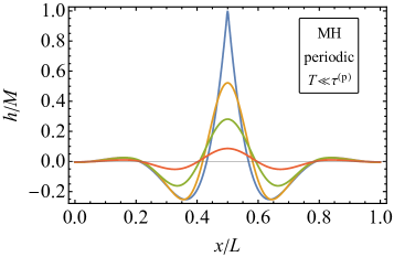
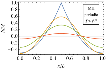
Figure 8: Time evolution of the optimal profile [Eqs. 58 and 59] for the MH equation with periodic boundary conditions in (a) the transient and (b) the equilibrium regime. The curves correspond, from center top to bottom, to (a) $1-t/T=0,0.1,0.4,0.8$ with $T=10^{-2}\tau^{\text{(p)}}$, and (b) $1-t/T=0,0.001,0.006,0.02$ with $T=100\tau^{\text{(p)}}$. Decreasing $T$ in (a) leads essentially to a reduction of the width of the curves [see also Eq. 68]. The fundamental time scale $\tau^{\text{(p)}}$ is reported in Eq. 54a.

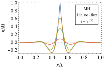
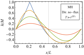
Figure 9: Time evolution of the optimal profile [Eq. 162] for the MH equation with Dirichlet no-flux boundary conditions in (a) the transient and (b) the equilibrium regime. The curves correspond, from center top to bottom, to (a) $1-t/T=0,0.05,0.3,0.8$ with $T=10^{-3}\tau^{(\mathrm{D}^{\prime})}$ and (b) $1-t/T=0,10^{-4},0.0025,0.01$ with $T=100\tau^{(\mathrm{D}^{\prime})}$. Decreasing $T$ in (a) leads essentially to a reduction of the width of the curves [see also Eq. 68]. The fundamental time scale $\tau^{(\mathrm{D}^{\prime})}$ is reported in Eq. 54b.

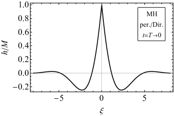
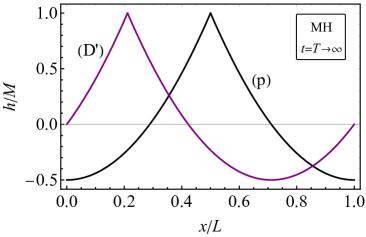
Figure 10: Asymptotic first-passage profiles $h(x,t=T)$ obtained within WNT of the MH equation for (a) the transient regime, $T\to 0$ [Eq. 66], and (b) the equilibrium regime, $T\to\infty$ [Eqs. 35a and 63]. In the transient regime, the profiles depend on the scaling variable $\xi\equiv(x-L/2)/(2T)^{1/4}$ and coincide for periodic and Dirichlet no-flux boundary conditions. The profiles for $T\to\infty$ follow from constrained minimization of the equilibrium action in Eq. 52. The equilibrium profiles at time $t=T$ for periodic and Dirichlet no-flux boundary conditions are related via a shift along $x$ [see Eq. 63].

For $T\gg\tau$, the profile at time $t=T$ minimizes the equilibrium action $\mathcal{S}_{\text{opt,eq}}$ [Eq. 52]. Since the latter quantity is independent of the specific dynamics, the expression for the profile $h^{\text{(p)}}(x,T)|_{T\to\infty}$ subject to periodic boundary conditions coincides with the one in Eq. 35a. Alternatively, it can be directly derived from the expression in Eq. 59 [see Eq. 194a]. In contrast to standard Dirichlet boundary conditions [see Eq. 35b as well as Fig. 13 in Appendix C], for Dirichlet no-flux boundary conditions one has to additionally take into account the constraint of zero mass [Eq. 11] in the minimization of $\mathcal{S}_{\text{opt,eq}}$. Accordingly, using the fact that $h(x,0)=0$, one obtains [see Eqs. 86 and 85]

$$h^{(\mathrm{D}^{\prime})}(x,T\to\infty)/M=h^{\text{(p)}}(x+L/2-x_{M},T\to\infty)/M=\begin{cases}\displaystyle 6\frac{x}{L}\left(\frac{x}{L}+\frac{1}{\sqrt{3}}\right),\qquad&x\leq x_{M}^{(\mathrm{D}^{\prime})},\\ \displaystyle 6\left(\frac{x}{L}-1\right)\left(\frac{x}{L}-1+\frac{1}{\sqrt{3}}\right),&x>x_{M}^{(\mathrm{D}^{\prime})},\end{cases}$$ (63)

with $x_{M}^{(\mathrm{D}^{\prime})}$ given in Eq. 57 and the last expression in Eq. 63 applying to the smaller of the two possible values of $x_{M}^{(\mathrm{D}^{\prime})}$. Note that, while, at the time $t=T$, $h^{(\mathrm{D}^{\prime})}$ can be expressed in terms of $h^{\text{(p)}}$, this is not possible at arbitrary times $t<T$, as, e.g., a close inspection of Fig. 8(b) and Fig. 9(b) near $h\approx 0$ reveals. In the equilibrium regime for nonzero but small time differences $\delta t\equiv T-t\ll T$, Eq. 58 can be cast into a dynamic scaling form [see Eq. 200]:

$$h(x,T-\delta t)\big{|}_{T\gg\tau}\simeq M-M(\delta t)^{1/z}\Gamma(1-1/z)\tilde{\mathcal{H}}\left(\frac{x-x_{M}}{\delta t^{1/z}}\right),\qquad z=4,$$ (64)

with the scaling function

$$\tilde{\mathcal{H}}(\xi)={}_{1}F_{3}\left(-\frac{1}{4};\frac{1}{4},\frac{1}{2},\frac{3}{4};\frac{\xi^{4}}{256}\right)+\xi^{2}\frac{\Gamma\left(\frac{1}{4}\right)}{8\Gamma\left(\frac{3}{4}\right)}{}_{1}F_{3}\left(\frac{1}{4};\frac{3}{4},\frac{5}{4},\frac{3}{2};\frac{\xi^{4}}{256}\right).$$ (65)

We recall that, in terms of the unscaled time variable, the argument of $\tilde{\mathcal{H}}$ in Eq. 64 is given by $(x-x_{M})/(\eta\,\delta t)^{1/z}$, which is dimensionless since $\eta$ and $L^{z}/T$ have the same dimensions. Asymptotically for $T\to 0$ in the transient regime, the profile at time $t=T$ is given by [see Eq. 180]:

$$h(x,T)\big{|}_{T\ll\tau}=M\mathcal{H}\left(\frac{x-L/2}{(2T)^{1/z}}\right),\qquad z=4,$$ (66)

with the scaling function

$$\mathcal{H}(\xi)={}_{1}F_{3}\left(-\frac{1}{4};\frac{1}{4},\frac{1}{2},\frac{3}{4};\frac{\xi^{4}}{256}\right)+\xi^{2}\frac{\Gamma\left(\frac{1}{4}\right)}{8\Gamma\left(\frac{3}{4}\right)}{}_{1}F_{3}\left(\frac{1}{4};\frac{3}{4},\frac{5}{4},\frac{3}{2};\frac{\xi^{4}}{256}\right)-\frac{\pi}{2\Gamma\left(\frac{3}{4}\right)}|\xi|.$$ (67)

For nonzero time differences $\delta t=T-t$ in the transient regime, a dynamic scaling profile follows at leading order in $\delta t/T\ll 1$ as [see Eq. 187]

$$h(x,T-\delta t)\big{|}_{\begin{subarray}{c}T\ll\tau\\ \delta t\ll T\end{subarray}}=M-M\left(\frac{\delta t}{2T}\right)^{1/z}\tilde{\mathcal{H}}\left(\frac{x-L/2}{\delta t^{1/z}}\right),\qquad z=4,$$ (68)

where the scaling function takes the same form as in Eq. 65. The scaling forms in Eqs. 64, 66 and 68 apply to both periodic and Dirichlet boundary conditions and are valid for values of the scaling variable $|\xi|\lesssim\mathcal{O}(1)$. [A comparison of the approximative profile in Eq. 68 with the exact one is provided in Fig. 14 in Appendix C, while a scaling form improving Eq. 68 beyond leading order in $\delta t/T$ is reported in Eq. 185.] In the case of periodic boundary conditions, the expressions in Eqs. 67 and 35a have been previously obtained in Ref. Meerson and Vilenkin (2016). Note that the static profile in the transient regime [Eq. 66] still depends on $T$ via the scaling variable $\xi$, whereas the static profile in the equilibrium regime [Eqs. 35a and 63] is independent of $T$ for sufficiently large $T$. The scaling profiles in Eqs. 66 and 68 have [in contrast to the exact solution in Eq. 59] nonzero mass [Eq. 9], which, however, constitutes a negligible error in the asymptotic limit $T\to 0$, where the profiles become sharply peaked. The profiles at time $t=T$ in the transient and the equilibrium regime are illustrated in Fig. 10.

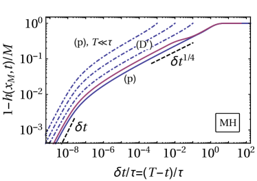
Figure 11: Time evolution of the peak of the profile $h(x_{M},t)$, which reaches the height $M$ at the first-passage time $T$, for the MH equation as a function of $T-t$. The solid curves correspond to $h^{\text{(p,D')}}(x_{M},t)$ in the equilibrium regime ($T\gg\tau$), while the dash-dotted curves illustrate the time evolution of $h^{\text{(p)}}(x_{M},t)$ in the transient regime for $T/\tau=10^{-1},10^{-2},10^{-3}$ (from bottom to top). Both in the transient and the equilibrium regime, a power law $M-h(x_{M},t)\propto\delta t^{1/4}$ is obtained as an intermediate asymptotic [see Eq. 69; dashed line]. If the number of modes in the system is finite, a linear behavior in $\delta t$ emerges for times $\delta t\lesssim\tau_{\times}$ [see Eq. 70], where $\tau_{\times}$ is the crossover time ($\tau_{\times}=0$ in the continuum limit). For illustrative purposes we have chosen here $\tau_{\times}/\tau\simeq 10^{-8}$. The fundamental time scale $\tau$ is defined in Eq. 54 for the respective boundary conditions.

According to Eqs. 64 and 68, noting that $\tilde{\mathcal{H}}(0)=1$, the peak $h(x_{M},t)$ of the profile approaches the maximum height $M$ via a power law

$$1-h(x_{M},T-\delta t)/M\propto\delta t^{1/z},\qquad z=4.$$ (69)

This behavior applies to a continuum system both in the transient and the equilibrium regime and is independent of the specific boundary conditions. If, due to a microscopic cutoff, the mode spectrum of the system is bounded from above, Eq. 69 crosses over to a linear law,

$$1-h(x_{M},T-\delta t)/M\propto\delta t\qquad\text{for}\qquad\delta t\lesssim\tau_{\times},$$ (70)

where $\tau_{\times}$ is the crossover time. For periodic boundary conditions, $\tau_{\times}=\tau^{\text{(p)}}/k_{\times}^{z}$, while for Dirichlet no-flux boundary conditions, $\tau_{\times}^{(\mathrm{D}^{\prime})}=\tau^{(\mathrm{D}^{\prime})}(\omega_{1}/\omega_{k_{\times}})^{z}$, where $k_{\times}$ is the maximum mode index and $\omega_{k}$ denotes the eigenvalues in Eq. 105. The time evolution of $h(x_{M},t)$ is illustrated in Fig. 11, where the time is rescaled by the characteristic relaxation time $\tau$ defined in Eq. 54. As noted previously, in the equilibrium regime, the actual evolution of the profile towards the maximum occurs within a time interval $\tau$ before $T$. In the case of Dirichlet no-flux boundary conditions, the intermediate asymptotic regime described by Eq. 69 is seen to be of somewhat smaller size than for periodic boundary conditions. In the transient regime, a condition determining the weak-noise limit of Eq. 55 follows from Eq. 69 as $L\gg\frac{D}{\eta}\left(\frac{L}{M}\right)^{2}\gg\frac{D}{\eta}\omega_{1}^{2}$, with $\omega_{1}^{\text{(p)}}=2\pi$ and $\omega_{1}^{(\mathrm{D}^{\prime})}=4.73$ [see Eq. 54b]. In contrast, in the equilibrium regime, the weak-noise limit is realized for $L\gg\frac{D}{\eta}\left(\frac{L}{M}\right)^{2}$ and $\left(\frac{L}{M}\right)^{2}\ll\omega_{1}^{2}$.

IV Summary

In the present study, first-passage events of a one-dimensional interfacial profile $h(x,t)$, subject to the Edwards-Wilkinson (EW) or the (stochastic) Mullins-Herring (MH) equation, have been investigated analytically. The approach here is based on the weak-noise approximation of a Martin-Siggia-Rose/Janssen/de Dominicis path integral formulation of the corresponding Langevin equations [Eqs. 1 and 2] Bertini et al. (2015); Fogedby and Ren (2009); Ge and Qian (2012); Grafke et al. (2015); Meerson and Vilenkin (2016); Täuber (2014). A comparison to numerical solutions of the EW and MH equation beyond the weak-noise approximation will be provided in a separate paper. Minimization of the associated action yields the most-probable (“optimal”) profile which, starting from a flat initial configuration [Eq. 5], realizes the first-passage event $h(x_{M},T)=M$ at a specified time $T$ and a location $x_{M}$. Note that here the rare event dynamics is purely fluctuation-induced, i.e., there is no deterministic driving force involved — in contrast to, e.g., the classical problem Zwanzig (2001) of determining noise-activated transitions between energy minima.

The first-passage problem of the MH equation for periodic boundary conditions has been studied previously in Ref. Meerson and Vilenkin (2016). Extending that work, here we have investigated the influence of various boundary conditions on the spatio-temporal evolution of the optimal profile and discussed in detail its dynamic scaling behavior. Since the optimal profile is provided here in terms of a generic eigenfunction expansion [see Appendix C], the corresponding expressions can be readily specialized to other boundary conditions. We point out that, in order to ensure mass conservation [Eq. 9] for the MH equation with Dirichlet boundary conditions, a no-flux condition must be imposed [see Eqs. 7 and 8]. This renders the solution of the corresponding WNT technically involved, as the bi-harmonic operator is not self-adjoint anymore. Standard Dirichlet boundary conditions, instead, do not conserve mass and are studied here mainly in conjunction with the EW equation.

The ensuing rare event dynamics is phenomenologically distinct for first-passage times $T\ll\tau$ and $T\gg\tau$, corresponding to the transient (non-equilibrium) and the equilibrium regime, respectively. $\tau$ denotes the fundamental relaxation time of the model, which coincides with the characteristic time scale for the evolution of the first-passage event. In the equilibrium regime, the optimal profile at time $t=T$ minimizes the equilibrium action and depends sensitively on the boundary conditions as well as on possible conservation laws. In contrast, in the transient regime, boundary conditions and mass conservation have a negligible influence and the optimal profile is strongly localized. In fact, in the transient regime, the profile shape close to the first-passage event (i.e., for $t\to T$) depends only on the type of bulk dynamics. The peak of the profile is predicted to approach the first-passage height $M$ algebraically in time, $M-h(x_{M},t)\propto(T-t)^{\alpha}$, with an exponent $\alpha=1/z$, where $z=2$ for the EW and $z=4$ for the MH equation. Notably, this behavior applies both in the transient and the equilibrium regimes and is independent of the specific boundary conditions or conservation laws.

Appendix A Equilibrium profiles

Here, we determine static profiles $h(x)$ ($0\leq x\leq L$) which minimize the equilibrium action [see Eqs. 21 and 52]

$$\mathcal{S}_{\text{eq}}[h]=\frac{\eta}{2D}\int_{0}^{L}\mathrm{d}x\,[\partial_{x}h(x)]^{2},$$ (71)

under the constraint of attaining a maximum height $M$ at a certain location $x_{M}$,

$$M=h(x_{M}).$$ (72)

In certain cases, we additionally impose a mass constraint:

$$\mathcal{A}=\int_{0}^{L}\mathrm{d}x\,h(x).$$ (73)

The profile $h$ is furthermore required to fulfill either periodic boundary conditions,

$$h(x)=h(x+L),$$ (74a)

or Dirichlet boundary conditions,

$$h(0)=0=h(L).$$ (74b)

Introducing Lagrange multipliers $\lambda$ and $\beta$, we obtain the augmented action

$$\tilde{\mathcal{S}}_{\text{eq}}([h],\lambda,\beta)\equiv\mathcal{S}_{\text{eq}}[h]-\lambda\left[\int_{0}^{L}\mathrm{d}x\,h(x)-\mathcal{A}\right]-\beta\left[\int_{0}^{L}\mathrm{d}x\,h(x)\,\delta\left(x-x_{M}\right)-M\right],$$ (75)

the minimization of which results in the Euler-Lagrange equation

$$0=\frac{\delta\tilde{\mathcal{S}}_{\text{eq}}}{\delta h}=\frac{\eta}{D}\partial_{x}^{2}h+\lambda+\beta\delta\left(x-x_{M}\right).$$ (76)

We remark that integration of Eq. 76 over an infinitesimal interval centered at $x_{M}$ yields the relation $h^{\prime}(x_{M}^{+})-h^{\prime}(x_{M}^{-})=\beta$, which, however, is not needed to determine the constrained profile. Instead, Eq. 76 is solved separately in the domains $x\lessgtr x_{M}$, subject to the boundary conditions in Eq. 74 and the requirement of continuity at $x_{M}$ [see Eq. 72], i.e.,

$$h(x_{M}^{+})=h(x_{M}^{-})=M.$$ (77)

Subsequently, the mass constraint in Eq. 73 is imposed. The expressions for the constrained profiles turn out to be independent of the factor $\eta/2D$ present in Eq. 71.

For $\mathcal{A}=0$ and periodic boundary conditions, setting $x_{M}=L/2$, one obtains the constrained profile Meerson and Vilenkin (2016)

$$h^{\text{(p)}}(x)/M=1-6\Bigg{|}\frac{x}{L}-\frac{1}{2}\Bigg{|}+6\left(\frac{x}{L}-\frac{1}{2}\right)^{2}.$$ (78)

For Dirichlet zero-$\mu$ boundary conditions [cf. Sec. B.1.3], we do not enforce the mass constraint [Eq. 73]. Accordingly, the Lagrange multiplier $\lambda$ is absent and one simply solves $0=\partial_{x}^{2}h$, subject to Eqs. 74b and 72, in each domain. The resulting solution still depends on $x_{M}$; the associated action, which is displayed in Fig. 2 in the main text, follows as

$$\frac{2D}{\eta}\frac{L}{M^{2}}\mathcal{S}_{\text{eq}}^{(\mathrm{D})}(x_{M})=\frac{1}{\zeta_{M}}+\frac{1}{1-\zeta_{M}},\qquad\text{with}\quad\zeta_{M}\equiv x_{M}/L.$$ (79)

$\mathcal{S}_{\text{eq}}^{(\mathrm{D})}$ is minimal for a value of

$$x_{M}^{(\mathrm{D})}=\frac{L}{2},$$ (80)

which finally leads to the constrained profile

$$h^{(\mathrm{D})}(x)/M=1-\left|1-\frac{2x}{L}\right|.$$ (81)

For Dirichlet no-flux boundary conditions, instead, the mass constraint is respected and, for $\mathcal{A}=0$, one obtains

$$h^{(\mathrm{D}^{\prime})}(x;x_{M})/M=\begin{cases}\displaystyle\frac{\zeta\left[1+3\,\zeta_{M}(\zeta-1)\right]}{\zeta_{M}\left[1+3\zeta_{M}(\zeta_{M}-1)\right]},\qquad&x\leq x_{M},\\ h^{(\mathrm{D}^{\prime})}(L-x,L-x_{M}),&x>x_{M},\end{cases}$$ (82)

with $\zeta\equiv x/L$ and $\zeta_{M}\equiv x_{M}/L$. Inserting Eq. 82 into Eq. 71 results in

$$\frac{2D}{\eta}\frac{L}{M^{2}}S_{\text{eq}}^{(\mathrm{D}^{\prime})}(x_{M})=\frac{1}{\zeta_{M}}+\frac{1}{1-\zeta_{M}}+\frac{3}{1+3\zeta_{M}(\zeta_{M}-1)},$$ (83)

which is illustrated in Fig. 7. This free energy has two symmetric minima, located at

$$x_{M}^{(\mathrm{D}^{\prime})}=\frac{L}{2}\left(1\pm\frac{1}{\sqrt{3}}\right).$$ (84)

The resulting optimal profile for Dirichlet no-flux boundary conditions and $\mathcal{A}=0$ is related to be $h^{\text{(p)}}$ [Eq. 78] via

$$h^{(\mathrm{D}^{\prime})}(x)=h^{\text{(p)}}(x+L/2-x_{M}^{(\mathrm{D}^{\prime})}).$$ (85)

Specifically, upon choosing the smaller value for $x_{M}^{(\mathrm{D}^{\prime})}$, one obtains

$$h^{(\mathrm{D}^{\prime})}(x)/M=\begin{cases}\displaystyle 6\zeta\left(\zeta+\frac{1}{\sqrt{3}}\right),\qquad&x\leq x_{M}^{(\mathrm{D}^{\prime})},\\ 6(\zeta-1)\left(\zeta-1+\frac{1}{\sqrt{3}}\right),&x>x_{M}^{(\mathrm{D}^{\prime})}.\end{cases}$$ (86)

Note that, since the above constrained profiles are polynomials of at most second order, one has $\partial_{x}^{(n)}h(x)=0$ for $n\geq 3$ in each domain $x\lessgtr x_{M}$, such that no-flux boundary conditions [see Eq. 8] are indeed fulfilled by $h^{(\mathrm{D}^{\prime})}$. In passing, we mention that, in the context of dewetting of thin films, related free-energy minimizing profiles have been considered in Refs. Bausch and Blossey (1994); Bausch et al. (1994); Blossey (1995); Foltin et al. (1997).

Appendix B Eigenvalue problem for the Mullins-Herring equation

Consider the noiseless MH equation,

$$\partial_{t}h(x,t)=-\partial_{x}^{4}h(x,t),$$ (87)

on the interval $[0,L]$ with

periodic: $$h(x,t)=h(x+L,t),$$ (88a)

Dirichlet: $$h(0,t)=0=h(L,t),$$ (88b)

or Neumann: $$\partial_{x}h(0,t)=0=\partial_{x}h(L,t),$$ (88c)

boundary conditions. The separation ansatz

$$h(x,t)=\sigma(x)\psi(t)$$ (89)

leads to

$$\partial_{t}\psi(t)=-\gamma\psi(t),$$ (90a)

$$\partial_{x}^{4}\sigma(x)=\gamma\sigma(x),$$ (90b)

with a constant $\gamma\geq 0$. While Eq. 90a is solved by

$$\psi(t)\sim e^{-\gamma t},$$ (91)

the general solution of the eigenvalue equation (90b) is given by

$$\sigma(x)=c_{1}e^{x\gamma^{1/4}}+c_{2}e^{-x\gamma^{1/4}}+c_{3}\sin(x\gamma^{1/4})+c_{4}\cos(x\gamma^{1/4})$$ (92)

with constants $c_{i}$, which are determined below for the specific boundary conditions.

To proceed, it is useful to introduce the free energy functional $\mathcal{F}[h]\equiv\int_{0}^{L}dx\,(\partial_{x}h)^{2}$ and the associated chemical potential $\mu\equiv\delta\mathcal{F}/\delta h=-\partial_{x}^{2}h$, which allows one to rewrite Eq. 87 as a “gradient-flow” equation Safran (1994):

$$\partial_{t}h=\partial_{x}^{2}\frac{\delta\mathcal{F}}{\delta h}=\partial_{x}^{2}\mu=-\partial_{x}\left[-\partial_{x}\mu\right].$$ (93)

In the last step we have identified $-\partial_{x}\mu$ as the flux, such that Eq. 93 takes the form of a continuity equation. Being a fourth order differential equation, Eq. 87 requires two additional conditions on $h$ beside those specified in Eq. 88. Here, one typically chooses either a vanishing chemical potential at the boundaries:

$$\mu(0,t)=0=\mu(L,t)\qquad\Leftrightarrow\qquad\sigma^{\prime\prime}(0)=0=\sigma^{\prime\prime}(L),$$ (94)

or a vanishing flux:

$$\partial_{x}\mu(0,t)=0=\partial_{x}\mu(L,t)\qquad\Leftrightarrow\qquad\sigma^{\prime\prime\prime}(0)=0=\sigma^{\prime\prime\prime}(L).$$ (95)

In contrast to the zero-chemical potential boundary conditions in Eq. 94, no-flux boundary conditions ensure mass conservation for the MH equation in a finite domain.

The type of boundary condition determines whether the operator $\partial_{x}^{4}$ is self-adjoint on the interval $[0,L]$ (see, e.g., Refs. Esposito and Kamenshchik (1999); Birkhoff (1908); Smith (2011)). Since, for two arbitrary functions $\sigma(x)$ and $\varphi(x)$, one has

$$\int_{0}^{L}\mathrm{d}x\,\sigma^{(4)}(x)\varphi(x)=[\sigma\varphi^{\prime\prime\prime}]_{0}^{L}-[\sigma^{\prime}\varphi^{\prime\prime}]_{0}^{L}+[\sigma^{\prime\prime}\varphi^{\prime}]_{0}^{L}-[\sigma^{\prime\prime\prime}\varphi]_{0}^{L}+\int_{0}^{L}\mathrm{d}x\,\sigma(x)\varphi^{(4)}(x),$$ (96)

the operator $\partial_{x}^{4}$ is self-adjoint only if both $\sigma$ and $\varphi$ fulfill either (i) periodic boundary conditions [Eq. 88a], (ii) Dirichlet zero-chemical potential boundary conditions [Eqs. 88b and 94], or (iii) Neumann no-flux boundary conditions [Eqs. 88c and 95]. In these cases, the eigenfunctions $\sigma_{m}$ defined by Eq. 90b, with $m\in\mathbb{Z}$ enumerating the spectrum, are orthogonal:

$$\int_{0}^{L}\mathrm{d}x\,\sigma_{m}^{*}(x)\sigma_{n}(x)=0,\qquad m\neq n.$$ (97)

In contrast, for Dirichlet no-flux boundary conditions [Eqs. 88b and 95], the boundary terms in Eq. 96 do not vanish. Consequently, $\partial_{x}^{4}$ is not self-adjoint on $[0,L]$ and the ensuing eigenfunctions $\sigma_{m}$ are not guaranteed to be orthogonal. This issue can be dealt with by introducing a set of eigenfunctions $\varphi_{m}(x)$ which solve the associated adjoint eigenproblem Birkhoff (1908). In the case of Dirichlet no-flux boundary conditions, this is defined by the eigenvalue equation

$$\partial_{x}^{4}\varphi(x)=\tilde{\gamma}\varphi(x)$$ (98)

and the boundary conditions

$$\varphi^{\prime}(0)= \,0=\varphi^{\prime}(L),$$ (99a)

$$\varphi^{\prime\prime}(0)= \,0=\varphi^{\prime\prime}(L).$$ (99b)

Note that these boundary conditions are indeed such that, upon using Eq. 95, all boundary terms in Eq. 96 vanish. In general, the (suitably ordered) proper and adjoint eigenvalues, $\gamma_{m}$ and $\tilde{\gamma}_{m}$, coincide Birkhoff (1908),

$$\gamma_{m}=\tilde{\gamma}_{m}.$$ (100)

This result is proven explicitly in Sec. B.1.1. Upon using this fact, Eq. 96 readily yields the mutual orthogonality of the proper and adjoint eigenfunctions $\sigma_{m}$, $\varphi_{n}$:

$$\int_{0}^{L}\mathrm{d}x\,\sigma_{m}^{*}(x)\varphi_{n}(x)=0,\qquad m\neq n.$$ (101)

This equation replaces Eq. 97 in the non-self-adjoint case and is crucial in constructing the eigenfunction solution of Eq. 87 or (53) for Dirichlet no-flux boundary conditions. We now proceed by discussing the eigenproblem of the MH equation for various boundary conditions.

B.1 Dirichlet boundary conditions

B.1.1 Vanishing flux

We consider here the proper eigenproblem defined by Eq. 90b and turn to the adjoint problem in the next subsection. Defining

$$\omega\equiv L\gamma^{1/4},$$ (102)

the four conditions in Eqs. 88b and 95 result in the requirement

$$\begin{pmatrix}1&1&0&1\\ e^{\omega}&e^{-\omega}&\sin(\omega)&\cos(\omega)\\ 1&-1&-1&0\\ e^{\omega}&-e^{-\omega}&-\cos(\omega)&\sin(\omega)\end{pmatrix}\begin{pmatrix}c_{1}\\ c_{2}\\ c_{3}\\ c_{4}\end{pmatrix}=\begin{pmatrix}0\\ 0\\ 0\\ 0\end{pmatrix}$$ (103)

for the coefficients $c_{i}$ defined in Eq. 92. For a nontrivial solution of Eq. 103 to exist, the determinant of the coefficient matrix must vanish, which implies

$$\cos(\omega)\cosh(\omega)=1.$$ (104)

In general, the solutions of Eq. 104 cannot be represented in a simple form. Numerically, one obtains

$$\omega_{k}=0,\,\pm 4.7300,\,\pm 7.8532,\,\pm 10.9956,\ldots\qquad(k=0,\pm 1,\pm 2,\ldots).$$ (105)

For $k\gtrsim 4$ the eigenvalues are well approximated by

$$|\omega_{k}|\simeq\pi\left(k+\frac{1}{2}\right),$$ (106)

which becomes exact in the limit $\omega\to\pm\infty$. Using Eq. 104, it can be shown that the eigenvalues $\omega_{k}$ fulfill the relation

$$\sin(\omega_{k})=\mathrm{sgn}\left(\omega_{k}\right)(-1)^{k}\sqrt{1-\frac{1}{\cosh^{2}(\omega_{k})}}.$$ (107)

Accordingly, Eq. 103 reduces to

$$\begin{pmatrix}1&1&0&1\\ e^{\omega_{k}}&e^{-\omega_{k}}&(-1)^{k}\tanh(\omega_{k})&1/\cosh(\omega_{k})\\ 1&-1&-1&0\\ e^{\omega_{k}}&-e^{-\omega_{k}}&-1/\cosh(\omega_{k})&(-1)^{k}\tanh(\omega_{k})\end{pmatrix}\begin{pmatrix}c_{1}\\ c_{2}\\ c_{3}\\ c_{4}\end{pmatrix}=\begin{pmatrix}0\\ 0\\ 0\\ 0\end{pmatrix},$$ (108)

which yields for the $c_{i}$ the nontrivial solutions

$$\begin{pmatrix}c_{1},c_{2},c_{3},c_{4}\end{pmatrix}_{k}=(\mathrm{sgn}\omega_{k})^{k}\begin{pmatrix}\displaystyle-\frac{(-1)^{k}}{\sqrt{3+3e^{2\omega_{k}}}},&\displaystyle-\frac{\sqrt{1+\tanh(\omega_{k})}}{\sqrt{6}},&\displaystyle\frac{-(-1)^{k}+e^{\omega_{k}}}{\sqrt{3+3e^{2\omega_{k}}}},&\displaystyle\frac{(-1)^{k}+e^{\omega_{k}}}{\sqrt{3+3e^{2\omega_{k}}}}\end{pmatrix}.$$ (109)

The eigenfunctions $\sigma_{k}(x)$ [Eq. 92] of the operator $\partial_{x}^{4}$ for Dirichlet no-flux boundary conditions thus result as

$$\sigma_{k}^{(\mathrm{D}^{\prime})}(x)=c_{1,k}e^{x\gamma_{k}^{1/4}}+c_{2,k}e^{-x\gamma_{k}^{1/4}}+c_{3,k}\sin(x\gamma_{k}^{1/4})+c_{4,k}\cos(x\gamma^{1/4}_{k}),$$ (110)

with the $c_{i,k}$ given in Eq. 109. It is straightforward to show that $\sigma_{k=0}^{(\mathrm{D}^{\prime})}(x)=0$ as well as $\sigma_{k}^{(\mathrm{D}^{\prime})}(x)=\sigma_{-k}^{(\mathrm{D}^{\prime})}(x)$ [cf. Eq. 105]. Hence, we can restrict $k$ to strictly positive values, such that the general solution of Eq. 87 reads

$$h^{(\mathrm{D}^{\prime})}(x,t)=\sum_{k=1}^{\infty}a_{k}e^{-\gamma_{k}t}\sigma_{k}^{(\mathrm{D}^{\prime})}(x),$$ (111)

with constants $a_{k}$. It is furthermore useful to note that $\sigma_{k}^{(\mathrm{D}^{\prime})}(L/2)=0$ for odd $k$. The eigenfunctions $\sigma_{k}^{(\mathrm{D}^{\prime})}$ are not normalized here, but instead one has

$$\int_{0}^{L}\mathrm{d}x\left[\sigma_{k}^{(\mathrm{D}^{\prime})}(x)\right]^{2}=\frac{L}{3}\left(1+\frac{(-1)^{k}}{\cosh\omega_{k}}-\frac{2}{\omega}\tanh(\omega_{k})\right).$$ (112)

Upon using Eqs. 104 and 107 it can be shown that the mass identically vanishes:

$$\int_{0}^{L}\mathrm{d}x\,\sigma_{k}^{(\mathrm{D}^{\prime})}(x)=0.$$ (113)

Consequently, the solution in Eq. 111 is only compatible with initial conditions having zero mass. [A nonzero mass can be trivially introduced by adding a constant to the r.h.s. of Eq. 111.] Moreover, it can be readily checked that, as a consequence of the non-self-adjoint character of $\partial_{x}^{4}$ for Dirichlet no-flux boundary conditions, the eigenfunctions $\sigma_{k}^{(\mathrm{D}^{\prime})}(x)$ are in general not orthogonal. This is the reason for considering an additional adjoint set of eigenfunctions (see below). In Fig. 12(a), the first few eigenfunctions defined by Eq. 110 are illustrated.

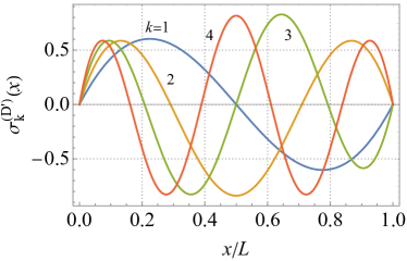
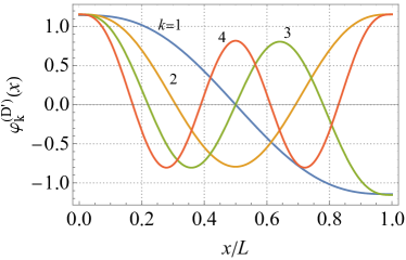
Figure 12: (a) Eigenfunctions $\sigma^{(\mathrm{D}^{\prime})}_{k}$ [Eq. 110] for Dirichlet no flux boundary conditions [Eqs. 88b and 95] for the four lowest modes $k=1,\ldots,4$. (b) Associated adjoint eigenfunctions $\varphi^{(\mathrm{D}^{\prime})}_{k}$ given by Eqs. 114 and 119. For $k=0$ one has $\sigma^{(\mathrm{D}^{\prime})}_{k=0}(x)=0$ and $\varphi^{(\mathrm{D}^{\prime})}_{k=0}(x)=2\sqrt{2/3}$.

B.1.2 Vanishing flux: adjoint eigenproblem

We now turn to the adjoint eigenvalue problem associated with Dirichlet no-flux boundary conditions, which is defined by Eqs. 98 and 99. The ansatz for the solution of the adjoint eigenvalue equation (98) is of the same form as in Eq. 92, i.e.,

$$\varphi(x)=\tilde{c}_{1}e^{x\tilde{\gamma}^{1/4}}+\tilde{c}_{2}e^{-x\tilde{\gamma}^{1/4}}+\tilde{c}_{3}\sin(x\tilde{\gamma}^{1/4})+\tilde{c}_{4}\cos(x\tilde{\gamma}^{1/4}).$$ (114)

The four conditions in Eq. 99 imply

$$\begin{pmatrix}1&-1&1&0\\ e^{\tilde{\omega}}&-e^{-\tilde{\omega}}&\cos(\tilde{\omega})&-\sin(\tilde{\omega})\\ 1&1&0&-1\\ e^{\tilde{\omega}}&e^{-\tilde{\omega}}&-\sin(\tilde{\omega})&-\cos(\tilde{\omega})\end{pmatrix}\begin{pmatrix}\tilde{c}_{1}\\ \tilde{c}_{2}\\ \tilde{c}_{3}\\ \tilde{c}_{4}\end{pmatrix}=\begin{pmatrix}0\\ 0\\ 0\\ 0\end{pmatrix}$$ (115)

for the coefficients $\tilde{c}_{i}$, where

$$\tilde{\omega}\equiv L\tilde{\gamma}^{1/4}.$$ (116)

Existence of a nontrivial solution of Eq. 103 implies the following determinant condition:

$$\cos(\tilde{\omega})\cosh(\tilde{\omega})=1.$$ (117)

As anticipated, this relation coincides with Eq. 104 and, consequently, also the adjoint and the proper eigenvalues [see Eq. 105] coincide:

$$\tilde{\omega}_{k}=\omega_{k}.$$ (118)

Proceeding as in Sec. B.1.1, one obtains the nontrivial solutions of Eq. 115 as

$$\begin{pmatrix}\tilde{c}_{1},\tilde{c}_{2},\tilde{c}_{3},\tilde{c}_{4}\end{pmatrix}_{k}=\begin{pmatrix}\displaystyle\frac{(-1)^{k}}{\sqrt{3+3e^{2\omega_{k}}}},&\displaystyle\frac{1}{\sqrt{6}}\sqrt{1+\tanh(\omega_{k})},&\displaystyle\frac{-(-1)^{k}+e^{\omega_{k}}}{\sqrt{3+3e^{2\omega_{k}}}},&\displaystyle\frac{(-1)^{k}+e^{\omega_{k}}}{\sqrt{3+3e^{2\omega_{k}}}}\end{pmatrix}.$$ (119)

Since the eigenfunctions $\varphi_{k}(x)$ resulting from Eqs. 114 and 119 are identical for $\pm\omega_{k}$, we consider henceforth only $\omega_{k}\geq 0$, i.e., $k\geq 0$. As a consequence of Eq. 118, the orthogonality property in Eq. 101 follows. Specifically, one has (note that $\sigma$ and $\varphi$ are real-valued)

$$\int_{0}^{L}\mathrm{d}x\,\sigma_{m}(x)\varphi_{n}(x)=\frac{L}{3}\left(1-\frac{(-1)^{n}}{\cosh(\omega_{n})}\right)\delta_{mn}.$$ (120)

Furthermore, one readily proves the useful property

$$\int_{0}^{L}\mathrm{d}x\,\varphi_{m}(x)\varphi_{n}^{\prime\prime}(x)=-\frac{L}{3}\omega_{n}^{2}\left(1-\frac{(-1)^{n}}{\cosh(\omega_{n})}\right)\delta_{mn}.$$ (121)

In Fig. 12(b), the first few adjoint eigenfunctions $\varphi_{k}$ are illustrated.

B.1.3 Vanishing chemical potential

For completeness, we summarize here the solution of the eigenproblem for Dirichlet boundary conditions with a vanishing chemical potential at the boundaries (also called Dirichlet zero-$\mu$ boundary conditions). Following the same steps as in Sec. B.1.1 renders the well-known normalized eigenfunctions

$$\sigma_{k}(x)=\sqrt{\frac{2}{L}}\sin(x\gamma_{k}^{1/4}),\qquad\gamma_{k}=\left(\frac{\pi k}{L}\right)^{4},\qquad k=0,1,2,\ldots.$$ (122)

Note that, since $\sigma_{k=0}(x)=0$, $k=0$ is not considered to be part of the actual eigenspectrum. In summary, the solution of Eq. 87 for Dirichlet zero-$\mu$ boundary conditions takes the well-known form

$$h^{(\mathrm{D})}(x,t)=\sum_{k=1}^{\infty}a_{k}e^{-\left(\frac{\pi k}{L}\right)^{4}t}\sqrt{\frac{2}{L}}\sin\left(\frac{\pi k}{L}x\right),$$ (123)

where the constants $a_{k}$ are determined by the initial conditions on $h^{(\mathrm{D})}$.

Requiring a constant chemical potential at the boundaries generally leads to a mass loss during the time evolution:

$$\int_{0}^{L}\mathrm{d}x\,h^{(\mathrm{D})}(x,t)=\sum_{k=1}^{\infty}a_{k}e^{-\left(\frac{\pi k}{L}\right)^{4}t}\times\begin{cases}\frac{2L}{\pi k},&\text{odd $k$},\\ 0,&\text{even $k$}.\end{cases}$$ (124)

One may wonder whether the coefficients $a_{k}$ can be chosen such that $h^{(\mathrm{D})}$ [Eq. 123] satisfies no-flux boundary conditions [Eq. 95]: requiring a vanishing third derivative of $h^{(\mathrm{D})}$ at the boundaries results in a relation involving the sum over all modes, e.g., for $x=0$ one has $0=\sum_{k=1}^{\infty}a_{k}\exp(-(\pi k/L)^{4}t)(\pi k/L)^{3}$. As is readily seen, it is not possible to choose the coefficients $a_{k}$ such that no-flux boundary conditions are ensured during the whole time evolution of $h^{(\mathrm{D})}$. This requires, instead, a specific set of basis functions.

B.2 Periodic boundary conditions

In the case of periodic boundary conditions [Eq. 88a], one has $c_{1}=c_{2}=0$ in Eq. 92 and $L\gamma_{n}^{1/4}=2\pi n$ with $n=0,1,2,\ldots$. This yields the well-known series expansion

$$h^{\text{(p)}}(x,t)=\sum_{k=-\infty}^{\infty}a_{k}e^{-\left(\frac{2\pi k}{L}\right)^{4}t}\sqrt{\frac{1}{L}}e^{\frac{2\pi\mathrm{i}k}{L}x}.$$ (125)

The parameters $a_{k}$ must fulfill $a_{-k}=a^{*}_{k}$ in order to ensure that $h^{\text{(p)}}$ is real-valued. Since $\int_{0}^{L}dx\,h^{\text{(p)}}(x,t)=a_{0}$, the mass [Eq. 9] is conserved in time.

B.3 Neumann boundary conditions

Imposing Neumann boundary conditions [Eq. 88c] in conjunction with a no-flux condition [Eq. 95] renders a solution of Eq. 87 in terms of standard Neumann eigenfunctions:

$$h^{\text{(N)}}(x,t)=\sum_{k=0}^{\infty}a_{k}e^{-\left(\frac{\pi k}{L}\right)^{4}t}\sqrt{\frac{2-\delta_{k,0}}{L}}\cos\left(\frac{\pi k}{L}x\right).$$ (126)

We shall, however, not discuss Neumann boundary conditions further.

Appendix C Solution of weak-noise theory for the optimal profile

Here, the general solution of Eqs. 23 and 53 is determined, following the approach outlined in Ref. Meerson and Vilenkin (2016) for periodic boundary conditions. Recall that a flat profile is assumed at the initial time [Eq. 5],

$$h(x,t=0)=0,$$ (127)

while the first-passage event at time $T$ is defined by the condition that $h$ attains its maximum height $M>0$ at the location $x_{M}$ [Eq. 4],

$$h(x_{M},T)=M.$$ (128)

However, for actually determining the solution of WNT, we neither explicitly enforce that $h$ does not reach the height $M$ before $T$, nor that the profile stays below $M$ for all $x\neq x_{M}$. Consequently, one has to check at the end of the calculation that the obtained solution fulfills these conditions. For sufficiently large $M$, this turns out to be the case.

We begin by casting Eqs. 23 and 53 into the common form

$$\partial_{t}h =(-\partial_{x}^{2})^{b}\,[\partial_{x}^{2}h+2p],$$ (129a)

$$\partial_{t}p =-(-\partial_{x}^{2})^{b}\partial_{x}^{2}p,$$ (129b)

where $b=0$ for EW dynamics and $b=1$ for MH dynamics. The profile $h(x,t)$ is assumed to fulfill either periodic or Dirichlet boundary conditions [see Eqs. 6 and 7]. For MH dynamics with Dirichlet boundary conditions, we additionally assume either a vanishing chemical potential [Eq. 94] or a vanishing flux [Eq. 95] at the boundaries. (In the main text, we focus only on the latter.) The profile is expanded into a set of eigenfunctions $\sigma_{k}$,

$$h(x,t)=\sum_{k}h_{k}(t)\sigma_{k}(x),$$ (130)

which are determined by the associated eigenvalue problem [see Appendix B],

$$\partial_{x}^{z}\sigma_{k}(x)=\gamma_{k}\sigma_{k}(x),$$ (131)

where the dynamic index $z=2b+2$. The conjugate field $p$ satisfies the boundary conditions of the associated adjoint eigenproblem [see Appendix B] and is accordingly expanded in terms of the adjoint eigenfunctions $\varphi_{k}$ as

$$p(x,t)=\sum_{k}p_{k}(t)\varphi_{k}(x).$$ (132)

The adjoint eigenfunctions $\varphi_{k}$ fulfill

$$\partial_{x}^{z}\varphi_{k}(x)=\gamma_{k}\varphi_{k}(x).$$ (133)

If the operator $\partial_{x}^{z}$ is self-adjoint on $[0,L]$, one has $\varphi_{k}=\sigma_{k}$. This is in particular the case for periodic or Dirichlet zero-$\mu$ boundary conditions, such that

$$\varphi_{k}^{\text{(p,D)}}=\sigma_{k}^{\text{(p,D)}}.$$ (134)

In contrast, for Dirichlet no-flux boundary conditions on $h$, the operator $\partial_{x}^{4}$ is not self-adjoint. In this case, the required adjoint eigenfunctions $\varphi_{k}^{(\mathrm{D}^{\prime})}$, which fulfill Neumann zero-$\mu$ boundary conditions [see Eq. 99], are provided in Sec. B.1.2 .

By construction, $\sigma_{m}$ and $\varphi_{n}$ are mutually orthogonal [see Eq. 101]

$$\int_{0}^{L}\mathrm{d}x\,\sigma_{m}^{*}(x)\varphi_{n}(x)=\kappa_{n}\delta_{mn},$$ (135)

where the star denotes complex conjugation and $\kappa_{n}$ is a real number. Complex conjugation is necessary here in order to also take into account complex-valued eigenfunctions, which occur in the case of periodic boundary conditions [see Eq. 125]. We furthermore have

$$\int_{0}^{L}\mathrm{d}x\,\varphi_{m}^{*}(x)\varphi_{n}^{\prime\prime}(x)=\epsilon_{n}\delta_{mn},$$ (136)

with a real number $\epsilon_{n}$. The relevant properties of $\sigma_{k}$, $\varphi_{k}$ are summarized in Table 1.

	periodic [Eq. 88a]	Dirichlet zero-$\mu$ [Eqs. (88b), (94)]	Dirichlet no-flux [Eqs. (88b), (95)] ($b=1$)†
$\partial_{x}^{z}$ self-adjoint	yes	yes	no
$\sigma_{k}$	$\displaystyle\frac{1}{\sqrt{L}}\exp\left(\frac{2\pi\mathrm{i}k}{L}x\right)$	$\displaystyle\sqrt{\frac{2}{L}}\sin\left(\frac{k\pi}{L}x\right)$	$\sigma_{k}^{(\mathrm{D}^{\prime})}$ [Eq. 110]
$\varphi_{k}$	$\sigma_{k}$	$\sigma_{k}$	$\varphi_{k}^{(\mathrm{D}^{\prime})}$ [Eq. 114]
$k$	$0,\pm 1,\pm 2,\ldots^{\ddagger}$	$1,2,3,\ldots$	$1,2,3,\ldots$
$\gamma_{k}$ [Eqs. (131), (133)]	$\displaystyle(-1)^{b+1}\left(\frac{2\pi k}{L}\right)^{z}$	$\displaystyle(-1)^{b+1}\left(\frac{k\pi}{L}\right)^{z}$	$(\omega_{k}/L)^{4}$ [Eq. 105]
$\kappa_{k}$ [Eq. 135]	1	1	$\displaystyle\frac{L}{3}\left(1-\frac{(-1)^{k}}{\cosh(L\gamma_{k}^{1/4})}\right)$ [Eq. 120]
$\epsilon_{k}$ [Eq. 136]	$\displaystyle\left[-|\gamma_{k}|^{1/2}\right]^{b}\kappa_{k}$, $\epsilon_{0}=0$	$\displaystyle\left[-|\gamma_{k}|^{1/2}\right]^{b}\kappa_{k}$	$-\gamma_{k}^{1/2}\kappa_{k}$ [Eq. 121]

Table 1: Eigenfunctions and related properties of the operator $\partial_{x}^{z}$ on the interval $[0,L]$ for various boundary conditions. The proper and adjoint eigenfunctions are denoted by $\sigma_{k}$ and $\varphi_{k}$, respectively, and they coincide if $\partial_{x}^{z}$ is self-adjoint. The dynamic index $z$ is related to the parameter $b$ via $z=2b+2$, with $b=0$ for EW dynamics and $b=1$ for MH dynamics [see Eq. 129]. ^†Dirichlet no-flux boundary conditions are considered only for $b=1$. Note that $\sigma_{k}^{(\mathrm{D}^{\prime})}$ and $\varphi_{k}^{(\mathrm{D}^{\prime})}$ are not normalized here, such that the system size $L$ appears in the corresponding expression for $\kappa_{k}$. ^‡Due to the mass constraint [Eq. 11], the zero mode ($k=0$) is absent from the actual solution for periodic boundary conditions [see Eq. 158 below].

To proceed, we insert the expansions given in Eqs. 130 and 132 into Eq. 129, multiply Eq. 129a by $\varphi_{k}^{*}$, Eq. 129b by $\sigma_{k}^{*}$, and make use of the orthogonality properties in Eqs. 135 and 136. This yields ordinary differential equations for the coefficients $h_{k}$ and $p_{k}$:

$$\dot{h}_{k} =(-1)^{b}\left(\gamma_{k}h_{k}+2p_{k}\hat{\epsilon}_{k}\right),$$ (137a)

$$\dot{p}_{k} =(-1)^{b+1}\gamma_{k}p_{k},$$ (137b)

with

$$\hat{\epsilon}_{k}\equiv\begin{cases}1,&b=0\\ \epsilon_{k}/\kappa_{k},&b=1.\end{cases}$$ (138)

Equation (137b) is solved by

$$p_{k}(t)=B_{k}\exp\left[(-1)^{b+1}\gamma_{k}t\right],$$ (139)

with integration constants $B_{k}$ determined below. The solution of Eq. 137a follows as

$$h_{k}(t)=\begin{cases}\displaystyle A_{k}\exp\left[(-1)^{b}\gamma_{k}t\right]-p_{k}(t)\frac{\hat{\epsilon}_{k}}{\gamma_{k}},\qquad&\gamma_{k}\neq 0\\ A_{k}+(-1)^{b}2\hat{\epsilon}_{k}B_{k}t,&\gamma_{k}=0.\end{cases}$$ (140)

As can be inferred from Table 1, the case $\gamma_{k}=0$ is only relevant for $k=0$ and periodic boundary conditions, where one obtains a linear dependence of $h_{0}$ on time for $b=0$ (EW dynamics), whereas $\hat{\epsilon}_{0}=0$ for $b=1$. Imposing the initial condition in Eq. 127 and using Eqs. 140 and 139 yields

$$B_{k}=\frac{\gamma_{k}}{\hat{\epsilon}_{k}}A_{k},\qquad(\gamma_{k}\neq 0),$$ (141)

while for $\gamma_{k}=0$ ($k=0$), one obtains $A_{0}=0$ and $B_{0}$ is left undetermined. Accordingly,

$$h_{k}(t)=\begin{cases}2A_{k}\sinh\left((-1)^{b}\gamma_{k}t\right),\qquad&\gamma_{k}\neq 0,\\ (-1)^{b}2\hat{\epsilon}_{0}B_{0}t,&\gamma_{k}=0,\end{cases}$$ (142)

from which readily follows that $h_{0}(t)=0$ for periodic boundary conditions and MH dynamics. Expanding the profile at the final time $T$ as

$$h(x,T)=\sum_{k}H_{k}\sigma_{k}(x),$$ (143)

provides the relations

$$A_{k}=\frac{H_{k}}{2\sinh\left((-1)^{b}\gamma_{k}T\right)},\qquad(\gamma_{k}\neq 0)$$ (144)

as well as $B_{0}=(-1)^{b}H_{0}/(2\hat{\epsilon}_{0}T)$ (for $\gamma_{0}=0$ and if $\hat{\epsilon}_{0}\neq 0$). Summarizing, in terms of the (yet undetermined) coefficients $H_{k}$, the solution of Eq. 137 is given, for $\gamma_{k}\neq 0$, by

$$h_{k}(t) =H_{k}\frac{\sinh\left((-1)^{b}\gamma_{k}t\right)}{\sinh\left((-1)^{b}\gamma_{k}T\right)},$$ (145a)

$$p_{k}(t) =H_{k}\frac{\gamma_{k}\exp\left(-(-1)^{b}\gamma_{k}t\right)}{2\hat{\epsilon}_{k}\sinh\left((-1)^{b}\gamma_{k}T\right)}.$$ (145b)

In the special case $\gamma_{0}=0$, $\hat{\epsilon}_{0}\neq 0$ ($k=0$), corresponding to EW dynamics with periodic boundary conditions, one has

$$h_{0}(t) =H_{0}\frac{t}{T},$$ (146a)

$$p_{0}(t) =(-1)^{b}\frac{H_{0}}{2\hat{\epsilon}_{0}T},$$ (146b)

whereas for $\gamma_{0}=0$, $\hat{\epsilon}_{0}=0$, corresponding to MH dynamics with periodic boundary conditions, one has

$$h_{0}(t) =0,$$ (147a)

$$p_{0}(t) =\mathrm{const}.$$ (147b)

In fact, performing the limit $\gamma_{k}\to 0$ in Eq. 145 leads to the expressions in Eq. 146. Furthermore, the fact that $h_{0}(t)=0$ for periodic boundary conditions and MH dynamics [see Eq. 142] implies $H_{0}=0$ in this case. This allows us to generally proceed by using Eq. 145, keeping in mind that $p_{0}(t)=0$ for periodic boundary conditions and MH dynamics [as this result does not readily follow from a limit of Eq. 145b].

The coefficients $H_{k}$ are determined by minimizing the (rescaled) action in Eqs. 24 and 48,

$$\mathcal{S}_{\text{opt}}[p]=(-1)^{b}\int_{0}^{T}\mathrm{d}t\int_{0}^{L}\mathrm{d}x\,p(\partial_{x}^{2b}p),$$ (148)

subject to the constraint in Eq. 128. Inserting the expansion defined in Eqs. 132 and 145b into $\mathcal{S}_{\text{opt}}$ and making use of the orthogonality property in Eq. 136 leads to

$$\mathcal{S}_{\text{opt}}=\sum_{k}\frac{\gamma_{k}\tilde{\epsilon}_{k}}{2\hat{\epsilon}_{k}^{2}\left[\exp\left(2(-1)^{b}\gamma_{k}T\right)-1\right]}|H_{k}|^{2}\equiv\sum_{k}N_{k}(T)|H_{k}|^{2},$$ (149)

where

$$\tilde{\epsilon}_{k}\equiv\begin{cases}\kappa_{k},\qquad&b=0,\\ \epsilon_{k},&b=1,\end{cases}$$ (150)

and the quantity $N_{k}(T)$ is introduced as a shorthand notation. Taking into account Eq. 143, the augmented action reads

$$\tilde{\mathcal{S}}_{\text{opt}}=\mathcal{S}_{\text{opt}}-\lambda\left[h(x_{M},T)-M\right]=\sum_{k}N_{k}(T)|H_{k}|^{2}-\lambda\left[\sum_{k}H_{k}\sigma_{k}(x_{M})-M\right],$$ (151)

where $\lambda$ is a Lagrange multiplier. Minimization of $\tilde{\mathcal{S}}_{\text{opt}}$ with respect to $H_{k}$, i.e., requiring $0=\delta\tilde{\mathcal{S}}_{\text{opt}}/\delta H_{k}$, results in

$$H_{k}^{*}=\frac{\lambda\sigma_{k}(x_{M})}{2N_{k}(T)}.$$ (152)

The complex conjugation in Eq. 152 is relevant only for periodic boundary conditions, where one has $H_{k}^{*}=H_{-k}$, $N_{-k}=N_{k}$, and $\varphi_{-k}=\varphi_{k}^{*}$ [which has also been used in Eq. 149]; for the other boundary conditions, $H_{k}^{*}=H_{k}$. Upon using Eqs. 128 and 143, one obtains the constraint-induced value of the Lagrange multiplier,

$$\lambda(T)=\frac{M}{\displaystyle\sum_{k}\frac{|\sigma_{k}(x_{M})|^{2}}{2N_{k}(T)}}.$$ (153)

The solution of Eq. 129 under the conditions in Eqs. 127 and 128 is thus given by

$$h(x,t)=\frac{M}{Q(x_{M},T,L)}\sum_{k}\frac{\hat{\epsilon}_{k}^{2}\left[\exp\left(2(-1)^{b}\gamma_{k}T\right)-1\right]}{\gamma_{k}\tilde{\epsilon}_{k}}\frac{\sinh\left((-1)^{b}\gamma_{k}t\right)}{\sinh\left((-1)^{b}\gamma_{k}T\right)}\sigma_{k}^{*}(x_{M})\sigma_{k}(x)$$ (154)

with

$$Q(x_{M},T,L)\equiv\sum_{k}\frac{|\sigma_{k}(x_{M})|^{2}}{2N_{k}(T)}=\sum_{k}|\sigma_{k}(x_{M})|^{2}\frac{\hat{\epsilon}_{k}^{2}\left[\exp\left(2(-1)^{b}\gamma_{k}T\right)-1\right]}{\gamma_{k}\tilde{\epsilon}_{k}}.$$ (155)

It is useful to note that $\displaystyle H_{k}=\frac{M\sigma_{k}^{*}(x_{M})}{2Q(x_{M},T,L)N_{k}(T)}$. For the boundary conditions considered here and $k\neq 0$, one has $\hat{\epsilon}_{k}^{2}/\tilde{\epsilon}_{k}=\epsilon_{k}^{b}/\kappa_{k}^{2}$, $\epsilon_{k}^{b}=\epsilon_{k}$ as well as $\epsilon_{k}/\gamma_{k}<0$ (see Table 1). We emphasize that in general $Q(T/\tau)$ is only proportional to the function $\mathpzc{Q}(T/\tau)$ defined in Eqs. 32, 34, 60 and 62 in the main text, because the latter results from Eq. 154 after performing some simplifications. According to Eqs. 132 and 145b, the conjugate field $p$ is given by

$$p(x,t)=\frac{M}{Q(x_{M},T,L)}\sum_{k}\frac{\exp\left((-1)^{b}\gamma_{k}T\right)}{\kappa_{k}\exp\left((-1)^{b}\gamma_{k}t\right)}\sigma_{k}^{*}(x_{M})\varphi_{k}(x).$$ (156)

Notably, this result implies that the initial and final configurations of $p(x,t)$ are fully determined by the corresponding ones for $h$ specified in Eqs. 127 and 128. The optimal action in Eq. 149 reduces to

$$\mathcal{S}_{\text{opt}}(x_{M},M,T,L)=\frac{M^{2}}{2Q(x_{M},T,L)},$$ (157)

which is most easily proven by using Eq. 145b and the expression for $H_{k}$ stated after Eq. 155. Recall that the above results pertain to rescaled fields and time [see Eq. 22]. In particular, $\mathcal{S}_{\text{opt}}$ in Eq. 157 gets multiplied by $\eta/D$ upon returning to dimensional variables [see Eq. 25].

C.1 Specialization to different boundary conditions

C.1.1 Periodic boundary conditions

In the case of EW dynamics with periodic boundary conditions, the mass constraint in Eq. 11 is explicitly imposed. Since $\int_{0}^{L}\mathrm{d}x\,\exp(\mathrm{i}kx)=L\delta_{k,0}$ for $k=2\pi n/L$ with $n\in\mathbb{Z}$, this constraint implies

$$h_{k=0}(t)=0=H_{k=0}$$ (158)

for the expansion coefficients defined in Eqs. 130 and 143. Since the profile $h(x,t)$ is real-valued, Eq. 130 yields $h^{*}=\sum_{k=-\infty}^{\infty}h^{*}_{k}\exp(-2\pi\mathrm{i}kx/L)=\sum_{k=-\infty}^{\infty}h_{-k}\exp(2\pi\mathrm{i}(-k)x/L)=h$ and thus

$$h_{k}^{*}=h_{-k}.$$ (159)

Furthermore, we have the symmetry property $N_{k}(T)=N_{-k}(T)$, as well as $\sigma_{k}(L/2)=(-1)^{k}/\sqrt{L}$ and $\sigma_{-k}(L/2)\sigma_{-k}(x)+\sigma_{k}(L/2)\sigma_{k}(x)=2(-1)^{k}\cos(2\pi kx/L)/L=2\cos(2\pi k(x/L-1/2))/L$. Accordingly, Eqs. 155 and 154 can be written as

$$h^{\text{(p)}}(x,t)=\frac{2M}{LQ^{\text{(p)}}(T,L)}\sum_{k=1}^{\infty}\frac{1-\exp\left(-2|\gamma_{k}|T\right)}{|\gamma_{k}|^{1-b/2}}\frac{\sinh\left(|\gamma_{k}|t\right)}{\sinh\left(|\gamma_{k}|T\right)}\cos\left(2\pi k(x/L-1/2)\right)$$ (160)

with

$$Q^{\text{(p)}}(T,L)=\frac{2}{L}\sum_{k=1}^{\infty}\frac{1-\exp\left(-2|\gamma_{k}|T\right)}{|\gamma_{k}|^{1-b/2}}.$$ (161)

The factor 2 arises since the sum originally includes also negative $k$. We have furthermore taken into account that, in the case of MH dynamics ($b=1$), the summand in Eqs. 160 and 161 vanishes for $k=0$ (which can be proven by carefully considering the limit $\gamma_{k}\to 0$), such that the zero mode is absent from the solution. In fact, Eq. 160 agrees with the expression obtained for MH dynamics in Ref. Meerson and Vilenkin (2016). In the case of EW dynamics without the mass constraint, the profile defined in Eq. 160 would superimpose onto a linear center-of-mass motion according to Eq. 146.

C.1.2 Dirichlet boundary conditions

Both for standard and no-flux Dirichlet boundary conditions, Eq. 154 assumes the generic expression

$$h^{\text{(D)}}(x,t)=\frac{M}{Q^{\text{(D)}}(x_{M},T,L)}\sum_{k=1}^{\infty}\frac{1-\exp\left(-2|\gamma_{k}|T\right)}{|\gamma_{k}|^{1-b/2}\kappa_{k}}\frac{\sinh\left(|\gamma_{k}|t\right)}{\sinh\left(|\gamma_{k}|T\right)}\sigma_{k}\left(x_{M}\right)\sigma_{k}(x)$$ (162)

with

$$Q^{\text{(D)}}(x_{M},T,L)=\sum_{k=1}^{\infty}\sigma_{k}^{2}\left(x_{M}\right)\frac{1-\exp\left(-2|\gamma_{k}|T\right)}{|\gamma_{k}|^{1-b/2}\kappa_{k}}.$$ (163)

If a vanishing chemical potential is imposed at the boundaries, the eigenfunctions are given by the standard Dirichlet ones, $\sigma_{k}^{(\mathrm{D})}(x)=\sqrt{2/L}\sin\left(\pi kx/L\right)$ with $\gamma_{k}=(\pi k/L)^{4}$. Taking $x_{M}=L/2$ [which is a convenient choice in the transient regime and minimizes the action in the equilibrium regime, see Eq. 80], one has

$$\sqrt{L/2}\,\sigma_{k}^{(\mathrm{D})}\left(L/2\right)=1,0,-1,0,1,\ldots$$ (164)

for $k=1,2,3,\ldots$, implying that only the odd modes contribute to the evolution of the profile. Furthermore, we note the useful relation

$$\sigma_{k}^{(\mathrm{D})}(L/2)\sigma_{k}^{(\mathrm{D})}(x)=\frac{2}{L}\cos\left(\frac{\pi k}{L}\left(x-\frac{L}{2}\right)\right),\qquad k=1,3,5,\ldots.$$ (165)

In the case of Dirichlet no-flux boundary conditions, the corresponding eigenfunctions $\sigma_{k}^{(\mathrm{D}^{\prime})}$ are reported in Eq. 110. Here, one has $\sigma_{k}^{(\mathrm{D}^{\prime})}(L/2)=0$ for odd $k$. In the equilibrium regime, $x_{M}$ as given in Eq. 84 has to be used instead of $L/2$.

The optimal profile $h^{(\mathrm{D}^{\prime})}(x,t)$ for MH dynamics with Dirichlet no-flux boundary conditions is discussed in the main text [see Eq. 61]. As a byproduct of the present analysis, we readily obtain the optimal profile $h^{(\mathrm{D})}(x,t)$ for MH dynamics with Dirichlet zero-$\mu$ boundary conditions, which is illustrated in Fig. 13. Mass is in general not conserved in this case. Introducing the time scale

$$\tau^{(\mathrm{D})}=\left(\frac{L}{\pi}\right)^{4},$$ (166)

the scaling form in Eq. 58 applies with

$$\mathpzc{h}^{(\mathrm{D})}(\mathrm{x},\mathrm{t},\mathrm{T})=\frac{1}{\mathpzc{Q}^{(\mathrm{D})}(\mathrm{T})}\sum_{k=1,3,5,\ldots}^{\infty}\frac{1-\exp\left(-2k^{4}\mathrm{T}\right)}{k^{2}}\frac{\sinh\left(k^{4}\mathrm{t}\right)}{\sinh\left(k^{4}\mathrm{T}\right)}\cos\left(\pi k\left(\mathrm{x}-1/2\right)\right)$$ (167)

and

$$\mathpzc{Q}^{(\mathrm{D})}(\mathrm{T})=\sum_{k=1,3,5,\ldots}^{\infty}\frac{1-\exp\left(-2k^{4}\mathrm{T}\right)}{k^{2}}.$$ (168)

The above expressions for $\mathpzc{h}$ and $\mathpzc{Q}$ in fact coincide with the corresponding ones in the EW case [Eqs. 31 and 33], except for the presence of $k^{2}$ instead of $k^{4}$.

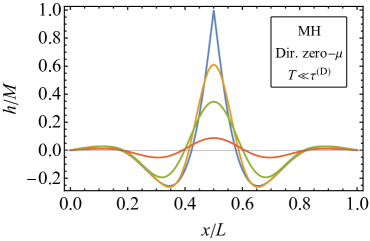
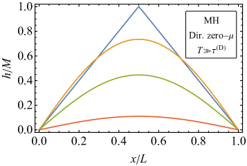
Figure 13: (a,b) Time evolution of the optimal profile for the MH equation with Dirichlet boundary conditions and a vanishing chemical potential at the boundaries [Eq. 162] in (a) the transient regime ($T=10^{-3}\tau^{(\mathrm{D})}$) and (b) the equilibrium regime ($T=100\tau^{(\mathrm{D})}$). The curves correspond from center top to bottom to (a) $1-t/T=0,0.05,0.3,0.8$ and (b) $1-t/T=0,10^{-5},10^{-4},5\times 10^{-4}$. The fundamental time scale is given by $\tau^{(\mathrm{D})}=(L/\pi)^{4}$.

C.2 Limiting cases

Introducing $\delta t\equiv T-t$, $\Gamma_{k}\equiv\epsilon_{k}/\gamma_{k}\kappa_{k}^{2}$ and using Table 1, Eq. 154 can be simplified to

$$h(x,\delta t)=\frac{M}{Q(T)}\sum_{k}\Gamma_{k}\left[\exp\left(-|\gamma_{k}|(2T-\delta t)\right)-\exp\left(-|\gamma_{k}|\delta t\right)\right]\sigma_{k}^{*}(x_{M})\sigma_{k}(x),$$ (169)

where we suppressed further arguments of $Q$ and note that $\Gamma_{k}<0$ as well as $(-1)^{b}\gamma_{k}=-|\gamma_{k}|$. Here and in the following, $h$ is considered to be a function of $\delta t$ instead of $t$. Specifically for $\delta t=0$, Eq. 169 reduces to

$$h(x,\delta t=0)=\frac{M}{Q(T)}\sum_{k}\Gamma_{k}\left[\exp(-2|\gamma_{k}|T)-1\right]\sigma_{k}^{*}(x_{M})\sigma_{k}(x).$$ (170)

Convenient analytical expressions for $h$ can be derived by replacing the sum in Eq. 169 by an integral using the Euler-Maclaurin formula. The error caused by this approximation is small if the summands in Eq. 169 vary significantly only over a few values of $k$. This is the case if $\delta t\ll\tau\simeq 1/|\gamma_{1}|$ (or, equivalently, $T\ll\tau$), since then the variation occurs for large $k$, where $|\gamma_{k}|\sim k^{z}$. [For $T\to\infty$, on the other hand, the first term in Eq. 169 can be neglected, see Sec. C.2.2.]

C.2.1 Transient regime ($T\ll\tau$)

Case $\delta t=0$. We first consider the case $\delta t=0$. For periodic boundary conditions, Eq. 170 becomes

$$\begin{split}h^{\text{(p)}}(x,\delta t=0)\big{|}_{T\ll\tau}&=\frac{2M}{LQ^{\text{(p)}}(T)}\left(\frac{L}{2\pi}\right)^{2}\sum_{k=1}^{\infty}\frac{1-\exp\left[-(2\pi k\,(2T)^{1/z}/L)^{z}\right]}{k^{2}}\cos\left(\frac{2\pi k}{L}(x-L/2)\right)\\ &\simeq\frac{(2T)^{1/z}M}{\pi\,Q^{\text{(p)}}(T)}\int_{0}^{\infty}\mathrm{d}y\frac{1-e^{-y^{z}}}{y^{2}}\cos(y\xi),\end{split}$$ (171)

with the fundamental integral

$$\int_{0}^{\infty}\mathrm{d}y\frac{1-e^{-y^{z}}}{y^{2}}\cos(y\xi)=\begin{cases}\displaystyle\sqrt{\pi}\exp\left(-\frac{\xi^{2}}{4}\right)+\frac{1}{2}\pi|\xi|\left[\mathrm{erf}\left(\frac{|\xi|}{2}\right)-1\right],\qquad z=2,\\ \displaystyle\Gamma\left(\frac{3}{4}\right){}_{1}F_{3}\left(-\frac{1}{4};\frac{1}{4},\frac{1}{2},\frac{3}{4};\frac{\xi^{4}}{256}\right)+\frac{1}{8}\Gamma\left(\frac{1}{4}\right)\xi^{2}{}_{1}F_{3}\left(\frac{1}{4};\frac{3}{4},\frac{5}{4},\frac{3}{2};\frac{\xi^{4}}{256}\right)-\frac{\pi}{2}|\xi|,\qquad z=4,\end{cases}$$ (172)

and $\xi\equiv(x-L/2)/(2T)^{1/z}$. Analogously, Eq. 161 evaluates to

$$\begin{split}Q^{\text{(p)}}(T\ll\tau)&=\frac{2}{L}\left(\frac{L}{2\pi}\right)^{2}\sum_{k=1}^{\infty}\frac{1-\exp\left(-[2\pi k\,(2T)^{1/z}/L]^{z}\right)}{k^{2}}\\ &\simeq\frac{(2T)^{1/z}}{\pi}\int_{0}^{\infty}\mathrm{d}y\frac{1-\exp(-y^{z})}{y^{2}}=\frac{(2T)^{1/z}}{\pi}\Gamma\left(1-1/z\right),\end{split}$$ (173)

where, in the intermediate steps, the integration variable $k$ has been substituted by $y=2\pi k(2T)^{1/z}/L$. The lower integration boundary has been sent to zero since we consider $T\to 0$, noting that the associated error is negligible because the integrand vanishes for $y\to 0$. Analogously, for Dirichlet zero-$\mu$ boundary conditions, using Eq. 165, we obtain from Eqs. 162, 163 and 170:

$$\begin{split}h^{(\mathrm{D})}(x,\delta t=0)\big{|}_{T\ll\tau}&=\frac{2M}{LQ^{\text{(D)}}(T)}\left(\frac{L}{\pi}\right)^{2}\sum_{j=0}^{\infty}\frac{1-\exp\left(-\left[\pi(2j+1)(2T)^{1/z}/L\right]^{z}\right)}{(2j+1)^{2}}\cos\left(\frac{(2j+1)\pi}{L}(x-L/2)\right)\\ &=\frac{(2T)^{1/z}M}{\pi Q^{\text{(D)}}(T)}\int_{0}^{\infty}\mathrm{d}y\frac{1-\exp(-{y^{z}})}{y^{2}}\cos(y\xi),\end{split}$$ (174)

with

$$\begin{split}Q^{(\mathrm{D})}(T\ll\tau)&=\frac{2}{L}\left(\frac{L}{\pi}\right)^{2}\sum_{j=0}^{\infty}\frac{1-\exp\left(-\left[\pi(2j+1)(2T)^{1/z}/L\right]^{z}\right)}{(2j+1)^{2}}\\ &=\frac{(2T)^{1/z}}{\pi}\int_{0}^{\infty}\mathrm{d}y\frac{1-\exp(-{y^{z}})}{y^{2}}=\frac{(2T)^{1/z}}{\pi}\Gamma\left(1-1/z\right).\end{split}$$ (175)

In order to evaluate the sum in Eq. 170 for Dirichlet no-flux boundary conditions, we assume a $k^{\prime}$ such that, for $k\geq k^{\prime}$, the eigenvalue $\gamma_{k}$ and the parameter $\kappa_{k}$ can be approximated by their respective asymptotic forms [see Eqs. 106 and 1]

$$\gamma^{(\mathrm{D}^{\prime})}_{k}\simeq\left(\frac{(k+1/2)\pi}{L}\right)^{4},\qquad\kappa_{k}\simeq\frac{L}{3}.$$ (176)

In the transient regime, we set $x_{M}=L/2$ [see Eq. 183 for justification] and thus have $\sigma_{k}^{(\mathrm{D}^{\prime})}(L/2)=0$ for odd $k$. For $T\ll(L/\omega_{k})^{4}\ll\tau^{(\mathrm{D}^{\prime})}$, terms with $k<k^{\prime}$ in the sum in Eq. 170 are exponentially small and can be neglected. For even $k$ with $k\geq k^{\prime}$, we approximate $\sigma_{k}^{(\mathrm{D}^{\prime})}$ by

$$\sigma^{(\mathrm{D}^{\prime})}_{k}(x)\simeq(-1)^{k/2}\frac{2}{3}\cos\left[\pi\left(k+\frac{1}{2}\right)\left(x-\frac{L}{2}\right)\right].$$ (177)

While this approximation does not respect Dirichlet no-flux boundary conditions, it captures the oscillatory behavior of the actual $\sigma^{(\mathrm{D}^{\prime})}_{k}$ well. A numerical comparison of the resulting scaling profile with the exact one justifies the above approximations a posteriori. Within the large $k$ approximation, we have $[\sigma_{k}^{(\mathrm{D}^{\prime})}(L/2)]^{2}\simeq 2/3$ for even $k$. Accordingly, one obtains

$$\begin{split}h^{(\mathrm{D}^{\prime})}(x,\delta t=0)\big{|}_{T\ll\tau}&\simeq\frac{2M}{LQ^{(\mathrm{D}^{\prime})}(T)}\left(\frac{L}{\pi}\right)^{2}\sum_{k\geq k^{\prime}}^{\infty}\frac{1-\exp\left(-\left[\pi(2j+1)(2T)^{1/4}/L\right]^{4}\right)}{(2j+1)^{2}}\cos\left(\frac{(2j+1)\pi}{L}(x-L/2)\right)\\ &\simeq\frac{(2T)^{1/4}M}{\pi Q^{(\mathrm{D}^{\prime})}(T)}\int_{0}^{\infty}\mathrm{d}y\frac{1-\exp(-y^{4})}{y^{2}}\cos(y\xi)\end{split}$$ (178)

and analogously

$$Q^{(\mathrm{D}^{\prime})}(T\ll\tau)=\frac{(2T)^{1/4}}{\pi}\Gamma\left(3/4\right).$$ (179)

As before, sending the lower integration boundary to zero is justified in the limit $T\to 0$. In summary, in the transient regime, the asymptotic expressions of the static profiles $h(x,\delta t=0)$ for periodic and Dirichlet boundary conditions are identical and reduce to

$$h(x,\delta t=0)\big{|}_{T\ll\tau}=M\mathcal{H}\left(\frac{x-L/2}{(2T)^{1/z}}\right),$$ (180)

with the scaling function

$$\mathcal{H}(\xi)=\begin{cases}\displaystyle\exp\left(-\frac{\xi^{2}}{4}\right)+\frac{1}{2}\sqrt{\pi}|\xi|\left[\mathrm{erf}\left(\frac{|\xi|}{2}\right)-1\right],\qquad z=2,\\ \displaystyle{}_{1}F_{3}\left(-\frac{1}{4};\frac{1}{4},\frac{1}{2},\frac{3}{4};\frac{\xi^{4}}{256}\right)+\xi^{2}\frac{\Gamma\left(\frac{1}{4}\right)}{8\Gamma\left(\frac{3}{4}\right)}{}_{1}F_{3}\left(\frac{1}{4};\frac{3}{4},\frac{5}{4},\frac{3}{2};\frac{\xi^{4}}{256}\right)-\frac{\pi}{2\Gamma\left(\frac{3}{4}\right)}|\xi|,\qquad z=4,\end{cases}$$ (181)

which has the limits $\mathcal{H}(0)=1$ and $\mathcal{H}(\xi\to\infty)=0$. The expression of $\mathcal{H}$ for $z=4$ coincides with the result for periodic boundary conditions reported in Ref. Meerson and Vilenkin (2016). The profile given by Eq. 180 does not respect mass conservation [Eq. 11] for finite $T$. This can be readily shown by computing the mass using the last expression in Eq. 174 before performing the integral over $y$. However, as $T\to 0$, the resulting error becomes negligible since the width of the profile rapidly shrinks.

The quantity $Q$ has been evaluated above for the particular choice $x_{M}=L/2$. Analogous calculations can in fact be performed for arbitrary $x_{M}$ with $0<x_{M}<L$, yielding

$$Q(x_{M},T\ll\tau)=(2T)^{1/z}\mathpzc{q}(x_{M}/(2T)^{1/z}),$$ (182)

with a scaling function $\mathpzc{q}$ that has the property $\mathpzc{q}(\zeta\to\infty)=\mathrm{const}$. Accordingly, the action in Eq. 157 behaves as (see also Ref. Meerson and Vilenkin (2016))

$$\mathcal{S}_{\text{opt}}(x_{M})\big{|}_{T\to 0}\propto T^{-1/z},$$ (183)

and becomes independent of $x_{M}$ for $0<x_{M}<L$ in the limit $T\to 0$. For $x_{M}\in\{0,L\}$, instead, Dirichlet boundary conditions imply $\sigma_{k}^{\text{(D,D')}}(x_{M})=0$ for all $k$, such that $Q^{\text{(D,D')}}(x_{M})$ [Eq. 163] vanishes identically at the boundaries, resulting in a divergence of $\mathcal{S}_{\text{opt}}^{\text{(D,D')}}(x_{M})$ for $x_{M}\in\{0,L\}$. The fact that $\mathcal{S}_{\text{opt}}$ is independent of $x_{M}$ asymptotically in the transient regime justifies the choice $x_{M}=L/2$ made above.

Case $\delta t>0$. In order to obtain dynamic scaling profiles for nonzero $\delta t$ with $\delta t\ll\tau$ and $T\ll\tau$, we rewrite Eq. 169 as

$$h(x,\delta t)=\frac{M}{Q(T)}\sum_{k}\Gamma_{k}\left\{\left[\exp\left(-|\gamma_{k}|(2T-\delta t)\right)-1\right]+\left[1-\exp\left(-|\gamma_{k}|\delta t\right)\right]\right\}\sigma_{k}^{*}(x_{M})\sigma_{k}(x).$$ (184)

Performing calculations analogous to those leading from Eq. 170 to Eq. 180, the corresponding dynamic scaling profile in the transient regime follows as

$$h(x,\delta t\ll\tau)\big{|}_{T\ll\tau}=M\left(1-\frac{\delta t}{2T}\right)^{1/z}\mathcal{H}\left(\frac{x-L/2}{(2T-\delta t)^{1/z}}\right)-M\left(\frac{\delta t}{2T}\right)^{1/z}\mathcal{H}\left(\frac{x-L/2}{(\delta t)^{1/z}}\right).$$ (185)

For $x=L/2$ and $\delta t\ll T$, Eq. 185 simplifies to $h(L/2,\delta t)\simeq M-[\delta t/(2T)]^{1/z}$. In order to obtain an analogous scaling form for $x\neq L/2$, we consider the expression

$$\left(\frac{2T}{\delta t}\right)^{1/z}\left[M-h(x,\delta t)\right]\simeq\left(\frac{2T}{\delta t}\right)^{1/z}M\left[1-\mathcal{H}\left(\xi\left(\frac{\delta t}{2T}\right)^{1/2}\right)+\left(\frac{\delta t}{2T}\right)^{1/z}\mathcal{H}(\xi)\right],\qquad\delta t\ll T,$$ (186)

where we introduced $\xi\equiv(x-L/2)/\delta t^{1/z}$. Expanding the r.h.s. in Eq. 186 to leading (i.e., zeroth) order in $\delta t/T$, keeping $\xi$ fixed, yields the desired scaling form:

$$h(x,\delta t\ll T)\big{|}_{T\ll\tau}\simeq M-M\left(\frac{\delta t}{2T}\right)^{1/z}\tilde{\mathcal{H}}\left(\frac{x-L/2}{(\delta t)^{1/z}}\right),$$ (187)

with

$$\tilde{\mathcal{H}}(\xi)=\begin{cases}\displaystyle\exp\left(-\frac{\xi^{2}}{4}\right)+\frac{1}{2}\sqrt{\pi}\,\xi\,\mathrm{erf}\left(\frac{\xi}{2}\right),\qquad z=2,\\ \displaystyle{}_{1}F_{3}\left(-\frac{1}{4};\frac{1}{4},\frac{1}{2},\frac{3}{4};\frac{\xi^{4}}{256}\right)+\xi^{2}\frac{\Gamma\left(\frac{1}{4}\right)}{8\Gamma\left(\frac{3}{4}\right)}{}_{1}F_{3}\left(\frac{1}{4};\frac{3}{4},\frac{5}{4},\frac{3}{2};\frac{\xi^{4}}{256}\right),\qquad z=4.\end{cases}$$ (188)

As shown in Fig. 14, the scaling form in Eq. 187 provides an accurate approximation to the full profiles [Eqs. 160 and 162] in a region around $x_{M}$. The size of this region increases as $\delta t/T\to 0$.

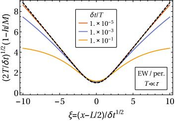
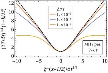
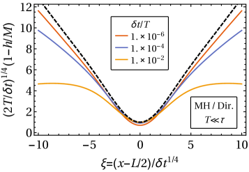
Figure 14: Scaling behavior in the transient regime for a profile subject to (a) EW and (b) MH dynamics with periodic boundary conditions, and (c) MH dynamics with Dirichlet no-flux boundary conditions. The dashed black curve represents the scaling function Eq. 188, while the solid curves represent the full expression of the profile in Eqs. 160 and 162, rescaled according to Eq. 187.

C.2.2 Equilibrium regime ($T\gg\tau$)

In the long-time limit, $T\to\infty$, the first term in the square brackets in Eq. 169 can be neglected, as can the exponential function in Eq. 170. Accordingly, $h$ becomes independent of $T$ and Eq. 169 reduces to

$$h_{\text{eq}}(x,\delta t)\equiv h(x,\delta t)\big{|}_{T\to\infty}=-\frac{M}{Q_{\text{eq}}}\sum_{k}\frac{\epsilon_{k}}{\gamma_{k}\kappa_{k}^{2}}\exp\left(-|\gamma_{k}|\delta t\right)\sigma_{k}(x_{M})\sigma_{k}(x),$$ (189)

with [see Eq. 155]

$$Q_{\text{eq}}=-\sum_{k}|\sigma_{k}(x_{M})|^{2}\frac{\epsilon_{k}}{\gamma_{k}\kappa_{k}^{2}}.$$ (190)

Case $\delta t=0$. For $\delta t=0$, the expressions in Eqs. 189 and 190 can be evaluated exactly in the case of periodic and Dirichlet zero-$\mu$ boundary conditions: according to Table 1, we have

$$Q_{\text{eq}}=\sum_{k}|\sigma_{k}(x_{M})|^{2}|\gamma_{k}|^{b/2-1}$$ (191)

as well as

$$h_{\text{eq}}(x,\delta t=0)=\frac{M}{Q_{\text{eq}}}\sum_{k}|\gamma_{k}|^{b/2-1}\sigma_{k}(x_{M})\sigma_{k}(x),$$ (192)

with $|\gamma_{k}^{\text{(p)}}|^{b/2-1}=(2\pi k/L)^{2}$ for periodic and $|\gamma_{k}^{(\mathrm{D})}|^{b/2-1}=(\pi k/L)^{2}$ for Dirichlet zero-$\mu$ boundary conditions, independently of the value of $b\in\{0,1\}$. Specifically, one obtains, invoking known Fourier series representations (see, e.g., Ref. Gradshteyn and Ryzhik (2014))

$$Q_{\text{eq}}^{\text{(p)}} =2L\sum_{k=1}^{\infty}\frac{1}{(2\pi k)^{2}}=\frac{L}{12},$$ (193a)

$$Q_{\text{eq}}^{(\mathrm{D})} =2L\sum_{k=1,3,5,\ldots}^{\infty}\frac{1}{(\pi k)^{2}}=\frac{L}{4},$$ (193b)

and analogously,

$$h_{\text{eq}}^{\text{(p)}}(x,\delta t=0)=\frac{2LM}{(2\pi)^{2}Q_{\text{eq}}^{\text{(p)}}}\sum_{k=1}^{\infty}\frac{\cos(2\pi k(x/L-1/2))}{k^{2}} =M\left[1-6\Bigg{|}\frac{x}{L}-\frac{1}{2}\Bigg{|}+6\left(\frac{x}{L}-\frac{1}{2}\right)^{2}\right],$$ (194a)

$$h_{\text{eq}}^{(\mathrm{D})}(x,\delta t=0)=\frac{2LM}{\pi^{2}Q_{\text{eq}}^{(\mathrm{D})}}\sum_{n=0}^{\infty}(-1)^{n}\frac{\sin((2n+1)\pi x/L)}{(2n+1)^{2}} =M-M\left|1-\frac{2x}{L}\right|,$$ (194b)

where we used Eq. 164. These expressions coincide with the ones in Eqs. 78 and 81 for the respective boundary conditions. A direct proof of the equivalence between $h_{\text{eq}}^{(\mathrm{D}^{\prime})}(x,\delta t=0)$ and the expression in Eq. 86 is not available owing to the non-algebraic dependence of $\omega$ on $k$ [see Eq. 104].

Case $\delta t>0$. For $T\to\infty$ and nonzero $\delta t\ll\tau$, asymptotic scaling profiles can be derived from Eq. 189 analogously to the calculation leading from Eq. 170 to Eq. 180. In the conversion of the sum to an integral, however, possible divergences have to be taken care of. In the case of periodic boundary conditions one obtains, taking $x_{M}=L/2$,

$$\begin{split}h^{\text{(p)}}(x,\delta t)\big{|}_{T\to\infty}&=\frac{2M}{LQ^{\text{(p)}}_{\text{eq}}}\left(\frac{L}{2\pi}\right)^{2}\sum_{k=1}^{\infty}\frac{\exp\left[-(2\pi k\,\delta t^{1/z}/L)^{z}\right]}{k^{2}}\cos\left(\frac{2\pi k}{L}(x-L/2)\right)\\ &\simeq\frac{(\delta t)^{1/z}M}{\pi\,Q^{\text{(p)}}_{\text{eq}}}\int_{Y_{1}}^{\infty}\mathrm{d}y\frac{e^{-y^{z}}}{y^{2}}\cos(y\xi),\end{split}$$ (195)

where $Y_{1}\equiv 2\pi(\delta t)^{1/z}/L$ and $\xi\equiv(x-L/2)/(\delta t)^{1/z}$ is a scaling variable. In order to take into account the singularity of the integral for $Y_{1}\to 0$, we write

$$\int_{Y_{1}}^{\infty}\mathrm{d}y\frac{e^{-y^{z}}}{y^{2}}\cos(y\xi)=\int_{Y_{1}}^{\infty}\mathrm{d}z\frac{e^{-y^{z}}-1}{y^{2}}\cos(y\xi)+\int_{Y_{1}}^{\infty}\mathrm{d}y\frac{\cos(y\xi)}{y^{2}}.$$ (196)

In the first term on the r.h.s. the limit $Y_{1}\to 0$ can be performed, yielding Eq. 172 up to a sign. For the second term, we obtain

$$\int_{Y_{1}}^{\infty}\mathrm{d}y\frac{\cos(y\xi)}{y^{2}}=\frac{\cos(\xi Y_{1})}{Y_{1}}-\frac{1}{2}\pi|\xi|+\xi\,\mathrm{Si}(\xi Y_{1}),$$ (197)

where $\mathrm{Si}$ is the sine integral Olver et al. (2010). Since $\xi Y_{1}=2\pi(x/L-1/2)$, expanding to first order in $(x/L-1/2)$, using $\mathrm{Si}(\zeta)\simeq\zeta+\mathcal{O}(\zeta^{2})$, we obtain

$$\int_{0}^{\infty}\mathrm{d}y\frac{e^{-y^{z}}}{y^{2}}\cos(y\xi)\simeq\begin{cases}\displaystyle\frac{1}{Y_{1}}-\sqrt{\pi}\exp\left(-\frac{\xi^{2}}{4}\right)-\frac{1}{2}\pi\,\xi\,\mathrm{erf}\left(\frac{\xi}{2}\right),\qquad z=2,\\ \displaystyle\frac{1}{Y_{1}}-\Gamma\left(\frac{3}{4}\right){}_{1}F_{3}\left(-\frac{1}{4};\frac{1}{4},\frac{1}{2},\frac{3}{4};\frac{\xi^{4}}{256}\right)-\frac{1}{8}\Gamma\left(\frac{1}{4}\right)\xi^{2}{}_{1}F_{3}\left(\frac{1}{4};\frac{3}{4},\frac{5}{4},\frac{3}{2};\frac{\xi^{4}}{256}\right),\qquad z=4.\end{cases}$$ (198)

For consistency in the approximation, we calculate $Q_{\text{eq}}$ in Eq. 193 in an analogous fashion, obtaining

$$Q_{\text{eq}}^{\text{(p)}}\simeq\frac{L}{2\pi^{2}}\int_{1}^{\infty}\mathrm{d}k\,k^{-2}=\frac{L}{2\pi^{2}}.$$ (199)

Inserting Eqs. 198 and 199 in Eq. 195 yields

$$h(x,\delta t)\big{|}_{T\to\infty}\simeq M-M(\delta t)^{1/z}\Gamma(1-1/z)\tilde{\mathcal{H}}\left(\frac{x-L/2}{\delta t^{1/z}}\right),$$ (200)

with the scaling function $\tilde{\mathcal{H}}$ given in Eq. 188. Hence, asymptotically, the scaling functions in the transient and the equilibrium regime are identical. The calculation proceeds analogously for Dirichlet boundary conditions, yielding for $h_{\text{eq}}^{(\mathrm{D})}$ the same result as in Eq. 200. Moreover, Eq. 200 applies also to Dirichlet no-flux boundary conditions, since in the asymptotic regime, i.e., for $\xi\lesssim\mathcal{O}(1)$ with $\delta t\ll\tau$, the precise value of $x_{M}$ is irrelevant, despite Eq. 57.

C.2.3 Effect of an upper mode cutoff

Above results pertain to a continuum system, which can sustain an infinite number of eigenmodes. Conversely, the presence of a minimal length scale in the system (e.g., a lattice constant) gives rise to an upper bound on the mode spectrum. Accordingly, the sums in Eqs. 154 and 155 are bounded by a maximum mode index $k_{\times}$. Associated with this mode is a relaxation rate $\gamma_{k_{\times}}$, which defines a cross-over time

$$\tau_{\times}\equiv\frac{1}{\gamma_{k_{\times}}}.$$ (201)

In a system with a mode cutoff, for times $\delta t\ll\tau_{\times}$ and $\delta t\ll T$, Eq. 169 can be approximated as

$$\begin{split}h(x,\delta t\lesssim\tau_{\times})&\simeq\frac{M}{Q(T)}\sum_{k}^{k_{\times}}\Gamma_{k}\big{[}\exp\left(-2|\gamma_{k}|T\right)-1+|\gamma_{k}|\delta t\big{]}\sigma_{k}^{*}(x_{M})\sigma_{k}(x)\\ &=h(x,0)+\delta t\frac{M}{Q(T)}\sum_{k}^{k_{\times}}\Gamma_{k}|\gamma_{k}|\sigma_{k}^{*}(x_{M})\sigma_{k}(x)\,,\end{split}$$ (202)

where $h(x,0)$ is the static profile defined in Eq. 170. Note that the second term in the last line of Eq. 202 is negative owing to the sign of $\Gamma_{k}$. Hence, for a bounded mode spectrum, the algebraic time evolution (with exponent $1/z$) of the profile described by Eqs. 187 and 200 crosses over to a linear one in $\delta t$ for small times, $\delta t\lesssim\tau_{\times}$. This behavior applies both in the transient and the equilibrium regime, independently from the boundary conditions.

References

- Edwards and Wilkinson (1982) S. F. Edwards and D. R. Wilkinson, “The Surface Statistics of a Granular Aggregate,” Proc. Roy. Soc. Lond. A. Math. Phys. 381, 17 (1982).
- Mullins (1957) W. W. Mullins, “Theory of Thermal Grooving,” J. Appl. Phys. 28, 333 (1957).
- Herring (1950) C. Herring, “Effect of Change of Scale on Sintering Phenomena,” J. Appl. Phys. 21, 301 (1950).
- Krug (1997) J. Krug, “Origins of scale invariance in growth processes,” Adv. Phys. 46, 139 (1997).
- Majumdar and Dasgupta (2006) S. N. Majumdar and C. Dasgupta, “Spatial survival probability for one-dimensional fluctuating interfaces in the steady state,” Phys. Rev. E 73, 011602 (2006).
- Majumdar and Comtet (2005) S. N. Majumdar and A. Comtet, “Airy Distribution Function: From the Area Under a Brownian Excursion to the Maximal Height of Fluctuating Interfaces,” J. Stat. Phys. 119, 777 (2005).
- Kardar et al. (1986) M. Kardar, G. Parisi, and Y.-C. Zhang, “Dynamic Scaling of Growing Interfaces,” Phys. Rev. Lett. 56, 889 (1986).
- Davidovitch et al. (2005) B. Davidovitch, E. Moro, and H. A. Stone, “Spreading of Viscous Fluid Drops on a Solid Substrate Assisted by Thermal Fluctuations,” Phys. Rev. Lett. 95, 244505 (2005).
- Gruen et al. (2006) G. Gruen, K. Mecke, and M. Rauscher, “Thin-Film Flow Influenced by Thermal Noise,” J. Stat. Phys. 122, 1261 (2006).
- Elliott (1989) C. M. Elliott, “The Cahn-Hilliard Model for the Kinetics of Phase Separation,” in Mathematical Models for Phase Change Problems, International Series of Numerical Mathematics No. 88, edited by J. F. Rodrigues (Birkhäuser Basel, 1989) pp. 35–73.
- Note (1) We remark that, without a microscopic cutoff, the stochastic EW and MH equations yield a diverging variance of the one-point height distribution for spatial dimensions Smith et al. (2017); Krug (1997). In the one-dimensional case considered here, the two models are well defined even without a regularization at small-scales.
- Abraham and Upton (1989) D. B. Abraham and P. J. Upton, “Dynamics of Gaussian interface models,” Phys. Rev. B 39, 736 (1989).
- Racz et al. (1991) Z. Racz, M. Siegert, D. Liu, and M. Plischke, “Scaling properties of driven interfaces: Symmetries, conservation laws, and the role of constraints,” Phys. Rev. A 43, 5275 (1991).
- Antal and Racz (1996) T. Antal and Z. Racz, “Dynamic scaling of the width distribution in Edwards-Wilkinson type models of interface dynamics,” Phys. Rev. E 54, 2256 (1996).
- Barabasi and Stanley (1995) A.-L. Barabasi and H. E. Stanley, Fractal Concepts in Surface Growth (Cambridge University Press, Cambridge, 1995).
- Majaniemi et al. (1996) S. Majaniemi, T. Ala-Nissila, and J. Krug, “Kinetic roughening of surfaces: Derivation, solution, and application of linear growth equations,” Phys. Rev. B 53, 8071 (1996).
- Flekkoy and Rothman (1995) E. G. Flekkoy and D. H. Rothman, “Fluctuating Fluid Interfaces,” Phys. Rev. Lett. 75, 260 (1995).
- Flekkoy and Rothman (1996) E. G. Flekkoy and D. H. Rothman, “Fluctuating hydrodynamic interfaces: Theory and Simulation,” Phys. Rev. E 53, 1622 (1996).
- Taloni et al. (2012) A. Taloni, A. Chechkin, and J. Klafter, “Generalized elastic model: Thermal vs. non-thermal initial conditions —Universal scaling, roughening, ageing and ergodicity,” EPL 97, 30001 (2012).
- Gross and Varnik (2013) M. Gross and F. Varnik, “Interfacial roughening in nonideal fluids: Dynamic scaling in the weak- and strong-damping regime,” Phys. Rev. E 87, 022407 (2013).
- Halpin-Healy and Zhang (1995) T. Halpin-Healy and Y.-C. Zhang, “Kinetic roughening phenomena, stochastic growth, directed polymers and all that. Aspects of multidisciplinary statistical mechanics,” Phys. Rep. 254, 215 (1995).
- Pruessner (2004) G. Pruessner, “Drift Causes Anomalous Exponents in Growth Processes,” Phys. Rev. Lett. 92, 246101 (2004).
- Cheang and Pruessner (2011) S. Cheang and G. Pruessner, “The Edwards–Wilkinson equation with drift and Neumann boundary conditions,” J. Phys. A.: Math. Theor. 44, 065003 (2011).
- Krug et al. (1997) J. Krug, H. Kallabis, S. N. Majumdar, S. J. Cornell, A. J. Bray, and C. Sire, “Persistence exponents for fluctuating interfaces,” Phys. Rev. E 56, 2702 (1997).
- Majumdar and Bray (2001) S. N. Majumdar and A. J. Bray, “Spatial Persistence of Fluctuating Interfaces,” Phys. Rev. Lett. 86, 3700 (2001).
- Majumdar and Comtet (2004) S. N. Majumdar and A. Comtet, “Exact Maximal Height Distribution of Fluctuating Interfaces,” Phys. Rev. Lett. 92, 225501 (2004).
- Schehr and Majumdar (2006) G. Schehr and S. N. Majumdar, “Universal asymptotic statistics of maximal relative height in one-dimensional solid-on-solid models,” Phys. Rev. E 73, 056103 (2006).
- Rambeau and Schehr (2010) J. Rambeau and G. Schehr, “Extremal statistics of curved growing interfaces in 1+1 dimensions,” EPL 91, 60006 (2010).
- Bray et al. (2013) A. J. Bray, S. N. Majumdar, and G. Schehr, “Persistence and first-passage properties in nonequilibrium systems,” Adv. Phys. 62, 225 (2013).
- Meerson and Vilenkin (2016) B. Meerson and A. Vilenkin, “Macroscopic fluctuation theory and first-passage properties of surface diffusion,” Phys. Rev. E 93, 020102 (2016).
- Meerson et al. (2016) B. Meerson, E. Katzav, and A. Vilenkin, “Large Deviations of Surface Height in the Kardar-Parisi-Zhang Equation,” Phys. Rev. Lett. 116, 070601 (2016).
- Rowlinson and Widom (1982) J. S. Rowlinson and B. Widom, Molecular Theory of Capillarity (Dover Publications, 1982).
- Note (2) Results for the MH equation with standard Dirichlet boundary conditions are briefly summarized in Sec. C.1.2.
- Note (3) For standard Dirichlet boundary conditions, the chemical potential , instead of the flux , vanishes at the boundaries [see Sec. B.1.3].
- Freidlin and Wentzell (1998) M. I. Freidlin and A. D. Wentzell, Random perturbations of dynamical systems, 2nd ed., Grundlehren der Mathematischen Wissenschaften [Fundamental Principles of Mathematical Sciences], Vol. 260 (Springer-Verlag, New York, 1998).
- E et al. (2004) W. E, W. Ren, and E. Vanden-Eijnden, “Minimum action method for the study of rare events,” Comm. Pure Appl. Math. 57, 637 (2004).
- Luchinsky et al. (1998) D. G. Luchinsky, P. V. E. McClintock, and M. I. Dykman, “Analogue studies of nonlinear systems,” Rep. Prog. Phys. 61, 889 (1998).
- Martin et al. (1973) P. C. Martin, E. G. Siggia, and H. A. Rose, “Statistical dynamics of classical systems,” Phys. Rev. A 8, 423 (1973).
- Janssen (1976) H.-K. Janssen, “On a Lagrangean for classical field dynamics and renormalization group calculations of dynamical critical properties,” Z. Phys. B 23, 377 (1976).
- de Dominicis (1976) C. de Dominicis, “Techniques de renormalisation de la theorie des champs et dynamique des phenomènes critiques,” J. Phys. Colloq. 37, C1 (1976).
- Täuber (2014) U. C. Täuber, Critical Dynamics: A Field Theory Approach to Equilibrium and Non-Equilibrium Scaling Behavior (Cambridge University Press, 2014).
- Fogedby and Ren (2009) H. C. Fogedby and W. Ren, “Minimum action method for the Kardar-Parisi-Zhang equation,” Phys. Rev. E 80, 041116 (2009).
- Ge and Qian (2012) H. Ge and H. Qian, “Analytical mechanics in stochastic dynamics: most probable path, large-deviation rate function and hamilton–jacobi equation,” Int. J. Mod. Phys. B 26, 1230012 (2012).
- Grafke et al. (2015) T. Grafke, R. Grauer, and T. Schäfer, “The instanton method and its numerical implementation in fluid mechanics,” J. Phys. A.: Math. Theor. 48, 333001 (2015).
- Smith et al. (2017) N. R. Smith, B. Meerson, and P. V. Sasorov, “Local average height distribution of fluctuating interfaces,” Phys. Rev. E 95, 012134 (2017).
- Bertini et al. (2015) L. Bertini, A. De Sole, D. Gabrielli, G. Jona-Lasinio, and C. Landim, “Macroscopic fluctuation theory,” Rev. Mod. Phys. 87, 593 (2015).
- Gross (2017) M. Gross, “First-passage dynamics of linear stochastic interface models: numerical simulations and entropic repulsion effect,” (2017).
- Bausch and Blossey (1994) R. Bausch and R. Blossey, “Lifetime of undercooled wetting layers,” Phys. Rev. E 50, R1759 (1994).
- Bausch et al. (1994) R. Bausch, R. Blossey, and M. A. Burschka, “Critical nuclei for wetting and dewetting,” J. Phys. A: Math. Gen. 27, 1405 (1994).
- Blossey (1995) R. Blossey, “Nucleation at first-order wetting transitions,” Int. J. Mod. Phys. B 09, 3489 (1995).
- Foltin et al. (1997) G. Foltin, R. Bausch, and R. Blossey, “Critical holes in undercooled wetting layers,” J. Phys. A: Math. Gen. 30, 2937 (1997).
- Seemann et al. (2001) R. Seemann, S. Herminghaus, and K. Jacobs, “Dewetting Patterns and Molecular Forces: A Reconciliation,” Phys. Rev. Lett. 86, 5534 (2001).
- Thiele et al. (2001) U. Thiele, M. G. Velarde, and K. Neuffer, “Dewetting: Film Rupture by Nucleation in the Spinodal Regime,” Phys. Rev. Lett. 87, 016104 (2001).
- Thiele et al. (2002) U. Thiele, K. Neuffer, Y. Pomeau, and M. G. Velarde, “On the importance of nucleation solutions for the rupture of thin liquid films,” Coll. Surf. A 206, 135 (2002).
- Tsui et al. (2003) O. K. C. Tsui, Y. J. Wang, H. Zhao, and B. Du, “Some views about the controversial dewetting morphology of polystyrene films,” Eur. Phys. J. E 12, 417 (2003).
- Becker et al. (2003) J. Becker, G. Grün, R. Seemann, H. Mantz, K. Jacobs, K. R. Mecke, and R. Blossey, “Complex dewetting scenarios captured by thin-film models,” Nat. Mater. 2, 59 (2003).
- Fetzer et al. (2007) R. Fetzer, M. Rauscher, R. Seemann, K. Jacobs, and K. Mecke, “Thermal Noise Influences Fluid Flow in Thin Films during Spinodal Dewetting,” Phys. Rev. Lett. 99, 114503 (2007).
- Croll and Dalnoki-Veress (2010) A. B. Croll and K. Dalnoki-Veress, “Hole nucleation in free-standing polymer membranes: the effects of varying molecular architecture,” Soft Matter 6, 5547 (2010).
- Blossey (2012) R. Blossey, Thin Liquid Films, Theoretical and Mathematical Physics (Springer Netherlands, Dordrecht, 2012).
- Nguyen et al. (2014) T. D. Nguyen, M. Fuentes-Cabrera, J. D. Fowlkes, and P. D. Rack, “Coexistence of spinodal instability and thermal nucleation in thin-film rupture: Insights from molecular levels,” Phys. Rev. E 89, 032403 (2014).
- Duran-Olivencia et al. (2017) M. A. Duran-Olivencia, R. S. Gvalani, S. Kalliadasis, and G. A. Pavliotis, “Instability, rupture and fluctuations in thin liquid films: Theory and computations,” arXiv:1707.08811 (2017).
- Eggers (2002) J. Eggers, “Dynamics of Liquid Nanojets,” Phys. Rev. Lett. 89, 084502 (2002).
- E and Vanden-Eijnden (2010) W. E and E. Vanden-Eijnden, “Transition-Path Theory and Path-Finding Algorithms for the Study of Rare Events,” Ann. Rev. Phys. Chem. 61, 391 (2010).
- Kim and Netz (2015) W. K. Kim and R. R. Netz, “The mean shape of transition and first-passage paths,” J. Chem. Phys. 143, 224108 (2015).
- Delarue et al. (2017) M. Delarue, P. Koehl, and H. Orland, “Ab initio sampling of transition paths by conditioned Langevin dynamics,” J. Chem. Phys. 147, 152703 (2017).
- Li et al. (2012) T. Li, P. Zhang, and W. Zhang, “Numerical study for the nucleation of one-dimensional stochastic Cahn-Hilliard dynamics,” Comm. Math. Sci. 10, 1105 (2012).
- Belardinelli et al. (2016) D. Belardinelli, M. Sbragaglia, M. Gross, and B. Andreotti, “Thermal fluctuations of an interface near a contact line,” Phys. Rev. E 94, 052803 (2016).
- Onsager and Machlup (1953) L. Onsager and S. Machlup, “Fluctuations and irreversible processes,” Phys. Rev. 36, 1505 (1953).
- Note (4) Note that standard Dirichlet boundary conditions imply for , as can be inferred from the series representation in Eq. 123.
- Zwanzig (2001) R. Zwanzig, Non-equilibrium Statistical Mechanics (Oxford University Press, 2001).
- Safran (1994) S. A. Safran, Statistical Thermodynamics of Surfaces, Interfaces and Membranes, 1st ed. (Addison-Wesley Publishing, 1994).
- Esposito and Kamenshchik (1999) G. Esposito and A. Y. Kamenshchik, “Fourth-order operators on manifolds with a boundary,” Class. Quant. Grav. 16, 1097 (1999).
- Birkhoff (1908) G. D. Birkhoff, “Boundary value and expansion problems of ordinary linear differential equations,” Trans. Amer. Math. Soc. 9, 373 (1908).
- Smith (2011) D. A. Smith, Spectral theory of ordinary and partial linear differential operators on finite intervals, Ph.D. thesis, Reading (2011).
- Note (5) It turns out that the adjoint eigenmode does not contribute to the dynamics for Dirichlet no-flux boundary conditions and will therefore be neglected henceforth in the corresponding expansion in Eq. 132.
- Gradshteyn and Ryzhik (2014) I. S. Gradshteyn and I. M. Ryzhik, Table of Integrals, Series, and Products (Academic, London, 2014).
- Olver et al. (2010) F. W. J. Olver, D. W. Lozier, R. F. Boisvert, and C. W. Clark, NIST Handbook of Mathematical Functions, 1st ed. (Cambridge University Press, 2010).