A generating function and formulae defining the first-associated Meixner-Pollaczek polynomials

Abstract.

While considering nonlinear coherent states with anti-holomorphic coefficients $\bar{z}^{n}/\sqrt{x_{n}!}$, we identify as first-associated Meixner-Pollaczek polynomials the orthogonal polynomials arising from shift operators which are defined by the sequence $x_{n}=(n+1)^{2}$. We give a formula defining these polynomials by writing down their generating function. This also leads to construct a Bargmann-type integral transform whose kernel is given in terms of a $\Psi_{1}$ Humbert’s function.

Dedicated to the memory of Professor Ahmed Intissar (1952-2017)

^∗ Department of Mathematics, Faculty of Sciences, Ibn Zohr University,
P.O. Box. 8106, Agadir, Morocco.
^♭ Department of Mathematics, Faculty of Sciences and Technics (M’Ghila),
P.O. Box. 523, Béni Mellal, Morocco.

1. Introduction

Coherent states (CSs) were first discovered by Schrödinger [1] as wavepackets having dynamics similar to that of a classical particle submitted to a quadratic potential. They have arised from the study of the quantum harmonic oscillator to become very useful in different areas of physics. CSs are also present in the investigation of news nonclassical states of light and their properties. In a such studies, generalizations of the notion of CSs plays a central role where new concepts such as interferences in phase space and nonlinear coherent states (NLCSs) have emerged [2]. Furthermore, NLCSs which can be classified as an algebraic generalization of the canonical coherent states of the harmonic oscillator have become an important tool in quantum optics.

In this paper, we replace the factorial $n!$ in canonical CSs by a generalized factorial $x_{n}!=x_{1}\cdots x_{n}$ with $x_{0}=0\,\,$and$\,\,x_{n}=(n+1)^{2},\ n=1,2,...$ and we discuss the corresponding resolution of the identity. We proceed by a general method [3] to attach to these NLCSs a set of orthogonal polynomials that arise from the shift operators which are defined via the sequence $x_{n}.$ We identify these polynomials as the first-associated Meixner-Pollaczek polynomials which were first introduced in 1950 by Pollaczek [10] via a tree-terms recurrence relation. A part from this relation no other property seems to be known in the literature. Thus, we establish a formula for their generating function from which we derive their expressions in terms of Gauss hypergeometric functions ${}_{2}F_{1}$ and classical Meixner-Pollaczek polynomials. Finally, by exploiting the obtained material we construct a new Bargmann-type integral transform whose kernel is given in terms of a $\Psi_{1}$ Humbert’s confluent hypergeometric function.

The paper is organized as follows. In section 2, we summarize the construction of NLCSs as well as a procedure to associate to them a set of orthogonal polynomials. In section 3, we particularize the formalism of NLCSs for the sequence $(n+1)^{2}$ and we discuss the corresponding resolution of the identity as well as the attached orthogonal polynomials arising from shift operators. For these polynomials a generating function is obtained in section 4. Section 5 is devoted to define a new Bargmann-type transform.

2. NLCS and polynomials attached to shift operators

Let $\{x_{n}\}_{n=0}^{\infty},\,\,x_{0}=0$, be an infinite sequence of positive real numbers. Let $\lim_{n\rightarrow+\infty}x_{n}=R^{2}$, where $R>0$ could be finite or infinite, but not zero. We shall use the notation $x_{n}!=x_{1}x_{2}\cdots x_{n}$ and $x_{0}!=1$. For each $z\in\mathcal{D}$ some complex domain, a generalized version of canonical CS can be defined as ([6], p.146) :

(2.1) $$|z\rangle=\left(\mathcal{N}(z\bar{z})\right)^{-1/2}\sum\limits_{n=0}^{+\infty}\frac{\bar{z}^{n}}{\sqrt{x_{n}!}}|\phi_{n}\rangle,\quad z\in\mathcal{D}$$

where the kets $|\phi_{n}\rangle,\,\,n=0,1,2,...,\infty$, are an orthonormal basis in an arbitrary (complex, separable, infinite dimensional) Hilbert space $\mathcal{H}$ and

(2.2) $$\mathcal{N}(z\bar{z})=\sum\limits_{n=0}^{+\infty}\frac{(z\bar{z})^{n}}{x_{n}!},$$

is a normalization factor chosen so that the vectors $|z\rangle$ are normalized to one. These vectors $|z\rangle$ are well defined for all $z$ for which the sum $(\ref{2.3})$ converges, i.e. $\mathcal{D}=\{z\in\mathbb{C},|z|<R\}$. We assume that there exists a measure $d\nu$ on $\mathcal{D}$ ensuring the resolution of the identity

(2.3) $$\int_{\mathcal{D}}|z\rangle\langle z|d\nu(z,\bar{z})=1_{\mathcal{H}}.$$

Setting $d\nu(z,\bar{z})=\mathcal{N}(z\bar{z})d\eta(z,\bar{z})$, it is easily seen that in order for $(\ref{2.4})$ to be satisfied, the measure $d\eta$ should be of the form $d\eta(z,\bar{z})=\frac{1}{2\pi}d\theta d\lambda(\rho),\ z=\rho e^{i\theta}$. The measure $d\lambda$ solves the moment problem

(2.4) $$\int_{0}^{R}\rho^{2n}d\lambda(\rho)=x_{n}!,\quad n=0,1,2,...\ .$$

In most of practical situations, the support of the measure $d\eta$ is the whole domain $\mathcal{D}$, i.e., $d\lambda$ is supported on the entire interval $[0,R)$.

Following [2], to the above family of coherent states $(\ref{2.2})$ is naturally associated a set of polynomials $p_{n}(x)$, orthogonal with respect to some measure on the real line. Moreover, these polynomials may then be used to replace the kets $\left|\phi_{n}\right\rangle$ in $(\ref{2.2})$. To see this, define the generalized annihilation operator $A$ by its action ”à la Glauber” on the vector $\left|z\right\rangle$ as $A\left|z\right\rangle=z\left|z\right\rangle$ and its adjoint $A^{\ast}$. Their actions on the basis vectors $\left|\phi_{n}\right\rangle,\ n=0,1,2,...,$ are easily seen to be

(2.5) $$A\left|\phi_{0}\right\rangle = 0,$$

(2.6) $$A\left|\phi_{n}\right\rangle = \sqrt{x_{n}}\left|\phi_{n-1}\right\rangle,$$

(2.7) $$A^{\ast}\left|\phi_{n}\right\rangle = \sqrt{x_{n+1}}\left|\phi_{n+1}\right\rangle.$$

Note that $x_{n}$ are the eigenvalues of the self-adjoint operator $H:=A^{\ast}A$, with eigenvectors $\left|\phi_{n}\right\rangle$. We now define the operators,

(2.8) $$Q=\frac{1}{\sqrt{2}}(A+A^{\ast}),\ \ \ P=\frac{1}{i\sqrt{2}}(A-A^{\ast}),$$

which are analogues of standard position and momentum operators. The operator $Q$ acts on $\left|\phi_{n}\right\rangle$ as

(2.9) $$Q\left|\phi_{n}\right\rangle=\sqrt{\frac{x_{n}}{2}}\left|\phi_{n-1}\right\rangle+\sqrt{\frac{x_{n+1}}{2}}\left|\phi_{n+1}\right\rangle.$$

If now the sum $\sum_{n=0}^{\infty}x_{n}^{-1/2}$ diverges, the operator $Q$ is essentially self-adjoint and hence admits a unique self-adjoint extension, which we again denote by $Q$ (see [6], p.147 and references therein). Let $E_{x},\ x\in\mathbb{R}$, be the spectral family of $Q$, so that,

(2.10) $$Q=\int_{\mathbb{R}}xdE_{x}.$$

Thus there is a measure $d\omega(x)=d\left\langle\phi_{0}|E_{x}\phi_{0}\right\rangle$ on $\mathbb{R}$ such that the vectors $\left|\phi_{n}\right\rangle$ can be realized as elements $p_{n}(x)$ in $L^{2}(\mathbb{R},dw)$. Furthermore, on this Hilbert space, $Q$ is just the operator of multiplication by $x$ and consequently, the relation $(\ref{2.8})$ takes the form

(2.11) $$xp_{n}(x)=c_{n}p_{n-1}(x)+c_{n+1}p_{n+1}(x),\ \ \ c_{n}=\sqrt{\frac{x_{n}}{2}.}$$

This is a recursion relation, familiar from the theory of orthogonal polynomials and thus the functions $p_{n}(x)$ are polynomials satisfying

(2.12) $$\int_{\mathbb{R}}p_{n}(x)p_{m}(x)d\omega(x)=\left\langle\phi_{n}|\phi_{m}\right\rangle=\delta_{n,m}.$$

3. NLCS associated with the sequence $x_{n}=(n+1)^{2}$

According to $(\ref{2.2})$ we associate to the sequence of positive numbers $x_{0}=0\,\,\text{and}\,\,x_{n}=(n+1)^{2},\ n=1,2,...$ a set of NLCS by the following superposition

(3.1) $$\left|z\right\rangle:=\left(\mathcal{N}(z\bar{z})\right)^{-\frac{1}{2}}\sum_{n=0}^{+\infty}\frac{\bar{z}^{n}}{(n+1)!}\left|\phi_{n}\right\rangle,$$

of the orthonormal basis vectors $\left|\phi_{n}\right\rangle$ in a Hilbert space $\mathcal{H}$. From the condition

(3.2) $$1=\left\langle z|z\right\rangle=\left(\mathcal{N}(z\bar{z})\right)^{-1}\sum_{n=0}^{+\infty}\frac{(1)_{n}}{(2)_{n}(2)_{n}}\frac{(z\bar{z})^{n}}{n!},$$

we see that the normalization factor is given by

(3.3) $$\mathcal{N}(z\bar{z})=\frac{1}{(z\bar{z})^{2}}\left(I_{0}(2z\bar{z})-1\right),$$

$I_{0}$ being the modified Bessel function of the first kind ([11], p.44). The measure with respect to which these NLCS ensure the resolution of the identity of the Hilbert space $\mathcal{H}$ as

(3.4) $$\int_{\mathbb{C}}\left|z\right\rangle\left\langle z\right|d\nu(z)=\mathbf{1}_{\mathcal{H}},$$

has the form ([4], p.4):

(3.5) $$d\nu(z)=4K_{0}(2|z|)\left(I_{0}(2z\bar{z})-1\right)d\mu(z),$$

in terms of the MacDonald function $K_{0}$ ([7], p.183) and the Lebesgue measure $d\mu$ on $\mathbb{C}$.
Remark 3.1. Note that in view of $(\ref{A*})$ the ket $|\phi_{n}\rangle$ can be written as $|\phi_{n}\rangle=(A^{\ast})^{n}|\phi_{0}\rangle,$ so that the NLCS $(\ref{cs})$ may also be obtained by displacing the state $|\phi_{0}\rangle$ as

(3.6) $$|z\rangle=\frac{z(A^{\ast})^{-1}}{\sqrt{I_{0}(2z\bar{z})-1}}\left(I_{0}(2\bar{z}A^{\ast})-\mathbf{1}\right)|\phi_{0}\rangle,$$

where $\mathbf{1}$ is the identity operator and $(A^{\ast})^{-1}$ is a left inverse of $A^{\ast}$ given by $(A^{\ast})^{-1}=H^{-1}A$, where $H=A^{*}A$. Furthermore, to the sequence $x_{n}=(n+1)^{2}$ is attached a function such that $x_{n+1}=f(x_{n})$, with $f(u)=\left(1+\sqrt{u}\right)^{2}$. This function encodes a generalized Heisenberg algebra (GHA) whose generators $A$ and $A^{\ast}$ satisfy the commutation relation: $\left[A,A^{\ast}\right]=f(H)-H=2\sqrt{H}+1$ (see, [14]).

Now, we proceed to attach to the sequence $x_{n}=(n+1)^{2}$ a set of orthogonal polynomials via the three-terms recurrence relation

(3.7) $$xp_{n}(x)=\frac{n+2}{\sqrt{2}}p_{n+1}(x)+\frac{n+1}{\sqrt{2}}p_{n-1}(x).$$

Proposition 3.1. The polynomials satisfying $(\ref{gamma1})$ are the first-associated Meixner-Pollaczek polynomials denoted as

(3.8) $$p_{n}(x):=P_{n}^{(1/2)}\left(\frac{x}{\sqrt{2}},\frac{\pi}{2},1\right),$$

and obey the orthonormality relations

(3.9) $$\int_{\mathbb{R}}p_{m}(x)p_{n}(x)\omega(x)dx=\delta_{mn},\quad m,n=0,1,2,...,$$

where the weight function

(3.10) $$\omega(x)=\frac{2}{\pi}\left|\Gamma\left(\frac{3}{2}+i\frac{x}{\sqrt{2}}\right)\right|^{2}\left|\ {}_{2}F_{1}\left(1,1;\frac{3}{2}+i\frac{x}{\sqrt{2}};\frac{1}{2}\right)\right|^{-2}$$

is given in terms of the Gauss hypergeometric sum ${}_{2}F_{1}.$

This can be proved by comparing $(\ref{gamma1})$ with the recurrence relation given in the paper of Pollaczek ([10], p.2256) where one can see that polynomials $P_{n}^{(1/2)}\left(x/\sqrt{2},\pi/2,1\right)$ belong to a larger class of orthogonal polynomials, denoted $P_{n}^{(\lambda)}(y;\phi,c)$ and called the $c$-associated Meixner-Pollaczek polynomials. The latter ones satisfy

$$(n+c+1)P_{n+1}^{\lambda}(y;\phi,c)-2\left[(n+\lambda+c)\cos\phi+y\sin\phi\right]P_{n}^{\lambda}(y;\phi,c)+(n+2\lambda+c-1)P_{n-1}^{\lambda}(x;\phi,c)=0,$$

with conditions $0<\varphi<\pi,\ 2\lambda+c>0$ and $c\geq 0$ or $0<\phi<\pi,\ 2\lambda+c\geq 1$ and $c>-1$. For $c=0$, $P_{n}^{(\lambda)}(y;\phi,0)\equiv P_{n}^{(\lambda)}(y;\phi)$ are the well known Meixner-Pollaczek polynomials.

Up to our knowledge, a part from the three-terms recurrence relation and orthonormality as written in Pollaczek’s paper [10] no other property seems to be known. Here, we first note that the polynomial $P^{(1/2)}_{n}\left(\frac{x}{\sqrt{2}},\frac{\pi}{2},1\right)$ also admits a representation in terms of the operator $Q$ as follows. From $(\ref{2.8})$, the operator $Q$ can be represented in the $\left|\phi_{n}\right\rangle$ basis as the infinite tridiagonal matrix

(3.11) $$Q=\left(\begin{array}[]{cccccc}0&\frac{2}{\sqrt{2}}&0&0&0&\cdots\\ \frac{2}{\sqrt{2}}&0&\frac{3}{\sqrt{2}}&0&0&\cdots\\ 0&\frac{3}{\sqrt{2}}&0&\frac{4}{\sqrt{2}}&0&\cdots\\ 0&0&\frac{4}{\sqrt{2}}&0&\frac{5}{\sqrt{2}}&\cdots\\ 0&0&0&\frac{5}{\sqrt{2}}&0&\cdots\\ \vdots&\vdots&\vdots&\vdots&\vdots&\ddots\end{array}\right).$$

Let $Q_{n}$ be the truncated matrix consisting of the first $n$ rows and columns of $Q$. Then it follows that the first-associated Meixner-Pollaczek polynomial is just the characteristic polynomial (up to a scale factor) of $Q_{n}$. That is,

(3.12) $$P^{(1/2)}_{n}\left(\frac{x}{\sqrt{2}},\frac{\pi}{2},1\right)=\frac{2^{\frac{n}{2}}}{(n+1)!}det\left[xI_{n}-Q_{n}\right],$$

where $I_{n}$ is the $n\times n$ identity matrix. Explicitly,

(3.13) $$P^{(1/2)}_{n}\left(\frac{x}{\sqrt{2}},\frac{\pi}{2},1\right)=\frac{2^{\frac{n}{2}}}{(n+1)!}\left|\begin{array}[]{cccccccc}x&-\frac{2}{\sqrt{2}}&0&0&0&\cdots&0&0\\ -\frac{2}{\sqrt{2}}&x&-\frac{3}{\sqrt{2}}&0&0&\cdots&0&0\\ 0&-\frac{3}{\sqrt{2}}&x&-\frac{4}{\sqrt{2}}&0&\cdots&0&0\\ 0&0&-\frac{4}{\sqrt{2}}&x&-\frac{5}{\sqrt{2}}&\cdots&0&0\\ 0&0&0&-\frac{5}{\sqrt{2}}&x&\cdots&\vdots&\vdots\\ \vdots&\vdots&\vdots&\vdots&\vdots&\ddots&-\frac{n-1}{\sqrt{2}}&0\\ 0&0&0&0&\cdots&-\frac{n-1}{\sqrt{2}}&x&-\frac{n}{\sqrt{2}}\\ 0&0&0&0&\cdots&0&-\frac{n}{\sqrt{2}}&x\end{array}\right|.$$

The first polynomials of this family are given by

$$P^{(1/2)}_{0}\left(\frac{x}{\sqrt{2}},\frac{\pi}{2},1\right) = 1,$$

$$P^{(1/2)}_{1}\left(\frac{x}{\sqrt{2}},\frac{\pi}{2},1\right) = \frac{1}{\sqrt{2}}x,$$

$$P^{(1/2)}_{2}\left(\frac{x}{\sqrt{2}},\frac{\pi}{2},1\right) = \frac{1}{3}x^{2}-\frac{2}{3},$$

$$P^{(1/2)}_{3}\left(\frac{x}{\sqrt{2}},\frac{\pi}{2},1\right) = \frac{\sqrt{2}}{12}x^{3}-\frac{13}{12\sqrt{2}}x,$$

$$P^{(1/2)}_{4}\left(\frac{x}{\sqrt{2}},\frac{\pi}{2},1\right) = \frac{1}{30}x^{4}-\frac{29}{60}x^{2}+\frac{8}{15}.$$

Their graphs are given in Figure 1.

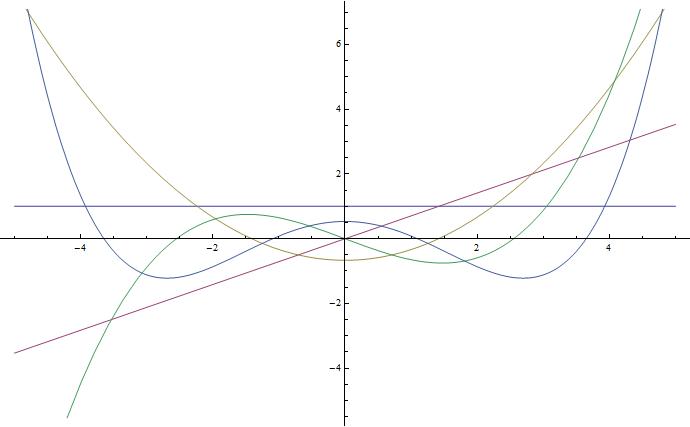
Figure 1. The polynomials $p_{0},p_{1},p_{2},p_{3}$ and $p_{4}$.

4. A generating function

In this section, we establish a formula for the generating function for the first-associated Meixner-Pollaczek polynomials, from which we derive an expression of these polynomials in terms of Meixner-Pollaczek polynomials and Gauss hypergeometric series ${}_{2}F_{1}$.

Theorem 4.1. A generating function for the first associated Meixner-Pollaczek polynomials is given by

$$\qquad\quad\sum\limits_{n\geq 0}P^{(1/2)}_{n}\left(\frac{x}{\sqrt{2}},\frac{\pi}{2},1\right)t^{n}=\frac{{}_{2}F_{1}\left(1,1;\frac{3+i\sqrt{2}x}{2};\frac{1+it}{2}\right)}{t(i-\sqrt{2}x)}+\frac{{}_{2}F_{1}\left(1,1;\frac{3+i\sqrt{2}x}{2};\frac{1}{2}\right)}{\sqrt{2}x-i}\frac{e^{\sqrt{2}x\arctan(t)}}{t\sqrt{t^{2}+1}},$$

for $|t|<1$ and $x\in\mathbb{R}$.

Proof. Let $p_{n}(x):=P_{n}^{(1/2)}\left(x/\sqrt{2},\pi/2,1\right)$ and denote by $G_{x}(t)$ the generating function $G_{x}(t):=\sum\limits_{n\geq 0}p_{n}(x)t^{n}$. Then, one can check that the function $t\mapsto G_{x}(t)$ satisfies the first order differential equation

(4.1) $$(t^{3}+t)G_{x}^{\prime}(t)+(2t^{2}-\sqrt{2}xt+1)G_{x}(t)-1=0$$

with the initial condition $G_{x}(0)=1$. Note that polynomials $p_{n}$ are not monic. However, the renormalized polynomials $q_{n}(x):=c_{n}!p_{n}(x)$ satisfy the recursion relation $q_{n+1}(x)=xq_{n}(x)-c_{n}^{2}q_{n-1}(x)$ from which it is clear that polynomials $q_{n}$ are indeed monic. We first establish a formula for the generating function of exponential type $\tilde{G}_{x}(t):=\sum_{n\geq 0}q_{n}(x)t^{n}/n!$, for polynomials $q_{n}$ satisfying the recurrence relation

(4.2) $$xq_{n}(x)=q_{n+1}(x)+\frac{(n+1)^{2}}{2}q_{n-1}(x).$$

By multiplying both sides of Eq.$(\ref{q_n})$ by $t^{n}/n!$ and summing over $n$, we see that the function $t\mapsto\tilde{G}_{x}(t)$ has to solve the second order differential equation

(4.3) $$(t^{2}+2)\tilde{G}^{{}^{\prime\prime}}_{x}(t)+(5t-2x)\tilde{G}^{{}^{\prime}}_{x}(t)+4\tilde{G}_{x}(t)=0.$$

We introduce the following change of variables $t=i\sqrt{2}(1-2\xi)$ and functions $\varphi(\xi):=\tilde{G}(x,i\sqrt{2}(1-2\xi))$. Then, Eq.$(\ref{equ.gener})$ reduces to the hypergeomertic differential equation

(4.4) $$\xi(1-\xi)\varphi^{\prime\prime}(\xi)+\left(\frac{5+i\sqrt{2}x}{2}-5\xi\right)\varphi^{\prime}(\xi)-4\varphi(\xi)=0,$$

whose solution is of the form ([5], p.256):

(4.5) $$\varphi(\xi)=\alpha\ {}_{2}F_{1}\left(\begin{array}[]{c}2,2\\ \frac{5+i\sqrt{2}x}{2}\end{array}\big{|}\xi\right)+\ \beta\xi^{\frac{-3-i\sqrt{2}x}{2}}\ {}_{2}F_{1}\left(\begin{array}[]{c}\frac{1-i\sqrt{2}x}{2},\frac{1-i\sqrt{2}x}{2}\\ \frac{-1-i\sqrt{2}x}{2}\end{array}\big{|}\xi\right)$$

where $\alpha,\beta$ are parameters depending on $x$ and ${}_{2}F_{1}$ denotes the Gauss hypergeometric function. In terms of the function $t\mapsto\tilde{G}_{x}(t)$, Eq.$(\ref{4.5})$ transforms to

$$\tilde{G}_{x}(t)=\alpha(x)\ \ {}_{2}F_{1}\left(\begin{array}[]{c}2,2\\ \frac{5+i\sqrt{2}x}{2}\end{array}\big{|}\frac{2+i\sqrt{2}t}{4}\right)+\beta(x)\left(\frac{2+i\sqrt{2}t}{4}\right)^{\frac{-3-i\sqrt{2}x}{2}}$$

$$\times\ {}_{2}F_{1}\left(\begin{array}[]{c}\frac{1-i\sqrt{2}x}{2},\frac{1-i\sqrt{2}x}{2}\\ \frac{-1-i\sqrt{2}x}{2}\end{array}\big{|}\frac{2+i\sqrt{2}t}{4}\right).$$

To determine $\alpha(x)$ and $\beta(x)$, we first make use of the Euler transformation ([8], p.313 ):

(4.6) $${}_{2}F_{1}\left(\begin{array}[]{c}a,b\\ c\end{array}\big{|}x\right)=(1-x)^{c-a-b}\ {}_{2}F_{1}\left(\begin{array}[]{c}c-a,c-b\\ c\end{array}\big{|}x\right)$$

for $a=\frac{1-i\sqrt{2}x}{2},\ \ b=\frac{1-i\sqrt{2}x}{2}$ and $c=\frac{-1-i\sqrt{2}x}{2}$, together with the identity

(4.7) $$\left(\frac{1-it}{1+it}\right)^{\frac{1}{2}iz}=\exp\left(z\arctan t\right),$$

for $z=\sqrt{2}x$. This gives

$$\tilde{G}_{x}(t)=\alpha(x)\ {}_{2}F_{1}\left(\begin{array}[]{c}2,2\\ \frac{5+i\sqrt{2}x}{2}\end{array}\big{|}\frac{2+i\sqrt{2}t}{4}\right)+\beta(x)(2x-t)(2+t^{2})^{-\frac{3}{2}}e^{\sqrt{2}x\arctan(\frac{t}{\sqrt{2}})}.$$

Next, the conditions $\tilde{G}_{x}(0)=1$ and $\tilde{G}_{x}^{\prime}(0)=x$ lead to the following system of equations

(4.8) $$\left\{\begin{array}[]{l}\alpha(x)\ {}_{2}F_{1}\left(\begin{array}[]{c}2,2\\ \frac{5+i\sqrt{2}x}{2}\end{array}\big{|}\frac{1}{2}\right)+\beta(x)(\sqrt{2})^{-1}x=1\\ \alpha(x)\frac{i2\sqrt{2}}{5+i\sqrt{2}x}\ {}_{2}F_{1}\left(\begin{array}[]{c}3,3\\ \frac{7+i\sqrt{2}x}{2}\end{array}\big{|}\frac{1}{2}\right)+\beta(x)(2\sqrt{2})^{-1}(2x^{2}-1)=x.\end{array}\right.$$

The solutions of $(\ref{4.9})$ are then obtained as

$$\alpha(x)=-\left[(2x^{2}-1){}_{2}F_{1}\left(\begin{array}[]{c}2,2\\ \frac{5+i\sqrt{2}x}{2}\end{array}\big{|}\frac{1}{2}\right)-\frac{4\sqrt{2}ix}{5+\sqrt{2}ix}{}_{2}F_{1}\left(\begin{array}[]{c}3,3\\ \frac{7+i\sqrt{2}x}{2}\end{array}\big{|}\frac{1}{2}\right)\right]^{-1},$$

and

$$\beta(x)=\frac{2^{\frac{3}{2}}x{}_{2}F_{1}\left(\begin{array}[]{c}2,2\\ \frac{5+i\sqrt{2}x}{2}\end{array}\big{|}\frac{1}{2}\right)-\frac{8i}{5+i\sqrt{2}x}{}_{2}F_{1}\left(\begin{array}[]{c}3,3\\ \frac{7+i\sqrt{2}x}{2}\end{array}\big{|}\frac{1}{2}\right)}{(2x^{2}-1){}_{2}F_{1}\left(\begin{array}[]{c}2,2\\ \frac{5+i\sqrt{2}x}{2}\end{array}\big{|}\frac{1}{2}\right)-\frac{4\sqrt{2}ix}{5+\sqrt{2}ix}{}_{2}F_{1}\left(\begin{array}[]{c}3,3\\ \frac{7+i\sqrt{2}x}{2}\end{array}\big{|}\frac{1}{2}\right)}.$$

To simplify the above expressions, we use the identity ([9], p.388):

(4.9) $$z(1-z)(a+1)(b+1)\ {}_{2}F_{1}\left(\begin{array}[]{c}a+2,b+2\\ c+2\end{array}\big{|}z\right)$$

$$+\newline (c-(a+b+1)z)(c+1)\ {}_{2}F_{1}\left(\begin{array}[]{c}a+1,b+1\\ c+1\end{array}\big{|}z\right)-c(c+1)\ {}_{2}F_{1}\left(\begin{array}[]{c}a,b\\ c\end{array}\big{|}z\right)=0$$

for $a=b=1,\ c=\frac{3+i\sqrt{2}x}{2},\ z=\frac{1}{2}$ and $a=b=0,\ c=\frac{1+i\sqrt{2}x}{2},z=\frac{1}{2}$. Therefore,

(4.10) $$\alpha(x)=\frac{1}{(1+i\sqrt{2}x)(3+i\sqrt{2}x)}\quad,\quad\beta(x)=\frac{2i}{1+i\sqrt{2}x}{}_{2}F_{1}(1,1;\frac{3+i\sqrt{2}x}{2};\frac{1}{2}).$$

Summarizing the above calculations, we obtain that

(4.11) $$\tilde{G}_{x}(t)=\left((1+i\sqrt{2}x)(3+i\sqrt{2}x)\right)^{-1}{}_{2}F_{1}\left(\begin{array}[]{c}2,2\\ \frac{5+i\sqrt{2}x}{2}\end{array}\big{|}\frac{1}{2}+i\frac{t}{2\sqrt{2}}\right)$$

$$+{}_{2}F_{1}\left(\begin{array}[]{c}1,1\\ \frac{3+i\sqrt{2}x}{2}\end{array}\big{|}\frac{1}{2}\right)\frac{(4x-2t)e^{\sqrt{2}x\arctan(\frac{t}{\sqrt{2}})}}{(\sqrt{2}x-i)(t^{2}+2)^{\frac{3}{2}}}$$

for every $x\in\mathbb{R}$. Using $(\ref{eq4.11})$ and the relation

(4.12) $$G_{x}(t)=\frac{t^{2}+1}{\sqrt{2}xt-t^{2}}\tilde{G}_{x}(\sqrt{2}t)+\frac{1}{t^{2}-\sqrt{2}xt}$$

connecting the two generating functions, we get

(4.13) $$\sum\limits_{n\geq 0}p_{n}(x)t^{n}=-\frac{1}{t(\sqrt{2}x-t)}+\frac{(t^{2}+1){}_{2}F_{1}\left(2,2;\frac{5+i\sqrt{2}x}{2};\frac{1+it}{2}\right)}{t(\sqrt{2}x-t)(1+i\sqrt{2}x)(3+i\sqrt{2}x)}$$

$$+\frac{{}_{2}F_{1}\left(1,1;\frac{3+i\sqrt{2}x}{2};\frac{1}{2}\right)}{\sqrt{2}x-i}\frac{e^{\sqrt{2}x\arctan(t)}}{t\sqrt{t^{2}+1}}.$$

Finally, we arrive at the expression $(\ref{GF new})$ by using the following equality

$$\frac{(t^{2}+1){}_{2}F_{1}\left(2,2;\frac{5+i\sqrt{2}x}{2};\frac{1+it}{2}\right)}{t(\sqrt{2}x-t)(1+i\sqrt{2}x)(3+i\sqrt{2}x)}=\frac{1}{t(\sqrt{2}x-t)}+\frac{{}_{2}F_{1}\left(1,1;\frac{3+i\sqrt{2}x}{2};\frac{1+it}{2}\right)}{t(i-\sqrt{2}x)}$$

which can be derived from $(\ref{F})$ by an appropriate choice of parameters.$\qquad\qquad\square$
Corollary 4.1. The following identity

(4.14) $${}_{2}F_{1}\left(\begin{array}[]{c}2,2\\ \frac{5}{2}\end{array}\big{|}\frac{1+it}{2}\right)=\frac{3}{t^{2}+1}\left[\frac{t}{\sqrt{t^{2}+1}}\left(\frac{i\pi}{2}-Log\left(t+\sqrt{t^{2}+1}\right)\right)+1\right]$$

holds true for $|t|<1$.
Proof. Evaluating at $x=0$ the closed form of the generating function as given in the right hand side of $(\ref{generatingfunction})$, leads to

(4.15) $$\sum_{n\geq 0}P_{n}^{(1/2)}\left(0,\frac{\pi}{2},1\right)t^{n}=\frac{2\sqrt{t^{2}+1}-it\pi}{2t^{2}\sqrt{t^{2}+1}}-\frac{t^{2}+1}{3t^{2}}{}_{2}F_{1}\left(\begin{array}[]{c}2,2\\ \frac{5}{2}\end{array}\big{|}\frac{1+it}{2}\right).$$

By another side, we use the recurrence relation $(\ref{gamma1})$ to get the following evaluations of polynomials $P_{n}^{(1/2)}\left(x,\frac{\pi}{2},1\right)$ at $x=0$ as

(4.16) $$\left\{\begin{array}[]{lll}P^{(1/2)}_{2n}\left(0,\frac{\pi}{2},1\right)=(-1)^{n}\frac{2^{2n}(n!)^{2}}{(2n+1)!},\\ P^{(1/2)}_{2n+1}\left(0,\frac{\pi}{2},1\right)=0.\end{array}\right.$$

This allows us to express the left hand side of $(\ref{generatingfunction})$ with $x=0$ as

(4.17) $$G_{0}(t)=\frac{1}{2t}\sum\limits_{n\geq 0}(-1)^{n}\frac{(n!)^{2}}{(2n+1)!}(2t)^{2n+1}.$$

To the later one, we apply the formula ([13], p.714):

(4.18) $$\sum\limits_{n\geq 0}(-1)^{n}\frac{(n!)^{2}}{(2n+1)!}u^{2n+1}=4(4+u^{2})^{-\frac{1}{2}}Log\left(\frac{u}{2}+\sqrt{\frac{u^{2}}{4}+1}\right),\ \ \ |u|<2,$$

for $u=2t$, to obtain an expression for $G_{0}(t)$ as

(4.19) $$G_{0}(t)=\frac{Log\left(t+\sqrt{t^{2}+1}\right)}{t\sqrt{t^{2}+1}},\qquad|t|<1.$$

By equating $(\ref{4.18})$ with $(\ref{g02})$, we arrive at the identity $(\ref{Hyp})$. $\square$

Remark 4.1. Using the fact that $i\arcsin(z)=Log(iz+\sqrt{1-z^{2}})$ in $(\ref{Hyp})$ and taking $t=-i(2\xi-1)$, we recover the identity ([12], p.481):

(4.20) $${}_{2}F_{1}\left(\begin{array}[]{c}2,2\\ \frac{5}{2}\end{array}\big{|}\xi\right)=\frac{3}{4\xi}\left(1-\xi\right)^{-1}\left[1-\frac{1-2\xi}{\sqrt{\xi(1-\xi)}}\arcsin\left(\sqrt{\xi}\right)\right].\vspace*{5mm}$$

Theorem 4.2. The first-associated Meixner-Pollaczek polynomials can be written as

$$P^{(1/2)}_{n}\left(x,\frac{\pi}{2},1\right)=\frac{i^{n}(2)_{n}\,{}_{2}F_{1}\left(n+2,n+2;n+\frac{5}{2}+ix;\frac{1}{2}\right)}{2^{n+2}\left(\frac{1}{2}+ix\right)_{n+2}}+\frac{{}_{2}F_{1}\left(1,1;\frac{3}{2}+ix;\frac{1}{2}\right)}{(2x-i)}P_{n+1}^{(1/2)}\left(x,\frac{\pi}{2}\right).$$

in terms of ${}_{2}F_{1}$-sums and Meixner-Pollaczek polynomials.
Proof. By multiplying by the variable $t$ the generating function $G_{x}(t)$ in $(\ref{GF new})$ as

$$tG_{x}(t)=\frac{{}_{2}F_{1}\left(1,1;\frac{3+i\sqrt{2}x}{2};\frac{1+it}{2}\right)}{(i-\sqrt{2}x)}+\frac{{}_{2}F_{1}\left(1,1;\frac{3+i\sqrt{2}x}{2};\frac{1}{2}\right)}{\sqrt{2}x-i}\frac{e^{\sqrt{2}x\arctan(t)}}{\sqrt{t^{2}+1}}$$

and denoting

(4.21) $$g_{x}(t):=\frac{e^{\sqrt{2}x\arctan(t)}}{\sqrt{t^{2}+1}}=\sum_{n=0}^{+\infty}P_{n}^{(1/2)}\left(\frac{x}{\sqrt{2}},\frac{\pi}{2}\right)t^{n},$$

the $(n+1)$ derivative of the function $t\longmapsto tG_{x}(t)$ reads

(4.22) $$\frac{\partial^{n+1}}{\partial t^{n+1}}\left(tG_{x}(t)\right)=\frac{i^{n}(2)_{n}(2)_{n}\,{}_{2}F_{1}\left(n+2,n+2;n+\frac{5+i\sqrt{2}x}{2};\frac{1+it}{2}\right)}{2^{n+1}\left(\frac{3+i\sqrt{2}x}{2}\right)_{n+1}(1+i\sqrt{2}x)}$$

$$+\frac{{}_{2}F_{1}\left(1,1;\frac{3+i\sqrt{2}x}{2};\frac{1}{2}\right)}{\sqrt{2}x-i}\frac{\partial^{n+1}}{\partial t^{n+1}}g_{x}(t).$$

By another hand, one has

(4.23) $$\frac{\partial^{n+1}}{\partial t^{n+1}}(tG_{x}(t))=(n+1)\frac{\partial^{n}}{\partial t^{n}}G_{x}(t)+t\frac{\partial^{n+1}}{\partial t^{n+1}}G_{x}(t).$$

From $(\ref{DG1})$-$(\ref{DG2})$, it then follows that

(4.24) $$(n+1)\frac{\partial^{n}}{\partial t^{n}}G_{x}(t)+t\frac{\partial^{n+1}}{\partial t^{n+1}}G_{x}(t)=$$

$$\frac{i^{n}(2)_{n}(2)_{n}\,{}_{2}F_{1}\left(n+2,n+2;n+\frac{5+i\sqrt{2}x}{2};\frac{1+it}{2}\right)}{2^{n+1}\left(\frac{3+i\sqrt{2}x}{2}\right)_{n+1}(1+i\sqrt{2}x)}+\frac{{}_{2}F_{1}\left(1,1;\frac{3+i\sqrt{2}x}{2};\frac{1}{2}\right)}{\sqrt{2}x-i}\frac{\partial^{n+1}}{\partial t^{n+1}}g_{x}(t).$$

Next, by evaluating the last equation at $t=0$ and using the fact that

(4.25) $$P^{(1/2)}_{n}\left(\frac{x}{\sqrt{2}},\frac{\pi}{2},1\right)=\frac{1}{n!}\frac{\partial^{n}}{\partial t^{n}}G_{x}(t)\mid_{t=0},$$

we arrive at

$$P^{(1/2)}_{n}\left(\frac{x}{\sqrt{2}},\frac{\pi}{2},1\right)=\frac{i^{n}(2)_{n}\,{}_{2}F_{1}\left(n+2,n+2;n+\frac{5+i\sqrt{2}x}{2};\frac{1}{2}\right)}{2^{n+2}\left(\frac{1+i\sqrt{2}x}{2}\right)_{n+2}}+\frac{{}_{2}F_{1}\left(1,1;\frac{3+i\sqrt{2}x}{2};\frac{1}{2}\right)}{(\sqrt{2}x-i)}P_{n+1}^{(1/2)}\left(\frac{x}{\sqrt{2}},\frac{\pi}{2}\right).$$

Finally, changing $x$ by $\sqrt{2}x$ completes the proof. $\square$

5. A Bargmann-type integral transform

Following ([2], p.4) the orthogonal polynomials $p_{n}(x)$ arising from the shift operators that are defined by the sequence $x_{n}$ may then be used to replace the abstract ket vectors $\left|\phi_{n}\right\rangle$ in $(\ref{2.2})$. In our case, this means that the obtained first-associated Meixner-Pollaczek polynomials $\left(\ref{Poly}\right)$ may define eigenstates of some explicit Hamiltonian operator. Such an operator could be determined by applying the method in [15] for example. In a such way, the wave functions of the resulting NLCSs as vectors in $L^{2}(\mathbb{R},\omega(x)dx)$, the Hilbert space spanned by the first-associated Meixner-Pollaczek polynomials, are of the form

(5.1) $$\langle\xi|z\rangle:=\left(\mathcal{N}(z\bar{z})\right)^{-1/2}\sum\limits_{n\geq 0}\frac{\overline{z}^{n}}{\sqrt{x_{n}!}}P_{n}^{(1/2)}\left(\frac{\xi}{\sqrt{2}},\frac{\pi}{2},1\right),\;\xi\in\mathbb{R}.$$

Proposition 5.1. The coordinate space representation of the NLCSs (5.1) is given by

(5.2) $$\langle\xi|z\rangle=\frac{ze^{-i\bar{z}}}{\sqrt{I_{0}(2z\bar{z})-1}(\sqrt{2}\xi-i)}\big{[}{}_{2}F_{1}\left(1,1;\frac{3+i\sqrt{2}\xi}{2};\frac{1}{2}\right){}_{1}F_{1}\left(\frac{1}{2}-\frac{i\xi}{\sqrt{2}},1;2i\bar{z}\right)$$

$$-\Psi_{1}\left(1,1;\frac{3+i\sqrt{2}\xi}{2},1;\frac{1}{2},i\bar{z}\right)\big{]}$$

for every $\xi\in\mathbb{R}$, in terms of the Humbert’s $\Psi_{1}$-series.
Proof. By using Theorem $4.2$, we replace polynomials in (5.1) by their explicit expressions. This gives

$$\mathcal{S}: = \sum_{n\geq 0}P_{n}^{(1/2)}\left(\frac{\xi}{\sqrt{2}},\frac{\pi}{2},1\right)\frac{\bar{z}^{n}}{(n+1)!}$$

$$= \frac{1}{2(1+i\sqrt{2}\xi)}\sum_{n\geq 0}\frac{{}_{2}F_{1}\left(n+2,n+2;n+\frac{5+i\sqrt{2}\xi}{2};\frac{1}{2}\right)}{2^{n}\left(\frac{3+i\sqrt{2}\xi}{2}\right)_{n+1}}(i\bar{z})^{n}$$

$$+ \frac{{}_{2}F_{1}\left(1,1;\frac{3+i\sqrt{2}\xi}{2};\frac{1}{2}\right)}{(\sqrt{2}\xi-i)}\sum_{n\geq 0}P_{n+1}^{(1/2)}\left(\frac{\xi}{\sqrt{2}},\frac{\pi}{2}\right)\frac{\bar{z}^{n}}{(n+1)!}$$

where the last sum in the R.H.S of the last equation involves a generating function for the classical Meixner-Pollaczek polynomials as follows

(5.4) $$\sum_{n\geq 0}P_{n+1}^{(1/2)}\left(\frac{\xi}{\sqrt{2}},\frac{\pi}{2}\right)\frac{\bar{z}^{n}}{(n+1)!}=\frac{1}{\bar{z}}e^{-i\bar{z}}{}_{1}F_{1}\left(\frac{1}{2}-\frac{i\xi}{\sqrt{2}},1;2i\bar{z}\right)-\frac{1}{\bar{z}}.$$

Therefore, the sum $\mathcal{S}$ in $(\ref{5.3})$ takes the form

$$\mathcal{S}=\frac{1}{\bar{z}(\sqrt{2}\xi-i)}\big{[}{}_{2}F_{1}\left(1,1;\frac{3+i\sqrt{2}\xi}{2};\frac{1}{2}\right)e^{-i\bar{z}}{}_{1}F_{1}\left(\frac{1}{2}-\frac{i\xi}{\sqrt{2}},1;2i\bar{z}\right)$$

(5.5) $$-\sum_{n\geq 0}\frac{1}{\left(\frac{3+i\sqrt{2}\xi}{2}\right)_{n}}\left(\frac{i\bar{z}}{2}\right)^{n}{}_{2}F_{1}\left(n+1,n+1;n+\frac{3+i\sqrt{2}\xi}{2};\frac{1}{2}\right)\big{]}.$$

For the remaining series in $(\ref{5.4})$, we prove that (see Appendix A):

$$\sum_{n\geq 0}\frac{1}{\left(\frac{3+i\sqrt{2}\xi}{2}\right)_{n}}\left(\frac{i\bar{z}}{2}\right)^{n}{}_{2}F_{1}\left(n+1,n+1;n+\frac{3+i\sqrt{2}\xi}{2};\frac{1}{2}\right)=e^{-i\bar{z}}\Psi_{1}\left(1,1;\frac{3+i\sqrt{2}\xi}{2},1;\frac{1}{2},i\bar{z}\right),$$

where $\Psi_{1}$ is a Humbert’s confluent hypergeometric function of two variables defined by ([16], p.126):

(5.6) $$\Psi_{1}(\alpha,\beta;\gamma,\gamma^{\prime};x,y)=\sum_{m,n\geq 0}\frac{(\alpha)_{m+n}(\beta)_{m}}{(\gamma)_{m}(\gamma^{\prime})_{n}}\frac{x^{m}}{m!}\frac{y^{n}}{n!},\qquad|x|<1.$$

Finally, recalling the expression of the prefactor $\mathcal{N}(z)$ in $(\ref{2.3})$ and summarizing the above calculations, we arrive at the announced result $(\ref{5.2})$. $\qquad\qquad\qquad\qquad\qquad\qquad\square$
Corollary 5.1. In addition, the function

(5.7) $$\Lambda(\xi,z):=\frac{\sqrt{I_{0}(2z\bar{z})-1}}{z\bar{z}}\langle\xi|\bar{z}\rangle=\displaystyle\sum_{n\geq 0}\frac{z^{n}}{\sqrt{x_{n}!}}P_{n}^{(1/2)}\left(\frac{\xi}{\sqrt{2}},\frac{\pi}{2},1\right),$$

is also a generating function for the first-associated Meixner-Pollaczek polynomials in the sense that

(5.8) $$P_{n}^{(1/2)}\left(\frac{\xi}{\sqrt{2}},\frac{\pi}{2},1\right)=(n+1)\frac{\partial^{n}}{\partial z^{n}}\Lambda(\xi,z)|_{z=0}.$$

Once we have obtained a closed form for the NLCSs (5.1) we can define the associated coherent states transform. The latter one should map the Hilbert space $L^{2}(\mathbb{R},\;\omega(x)dx)$ with

(5.9) $$\omega(x)=\frac{2}{\pi}\left|\Gamma\left(\frac{3}{2}+i\frac{x}{\sqrt{2}}\right)\right|^{2}\left|\ {}_{2}F_{1}\left(1,1;\frac{3}{2}+i\frac{x}{\sqrt{2}};\frac{1}{2}\right)\right|^{-2},$$

onto the Hilbert space $\mathcal{A}(\mathbb{C})$ of complex-valued analytic functions on $\mathbb{C}$, which are square integrable with respect to the measure $d\nu(z)=4(z\bar{z})^{2}K_{0}(2|z|)d\mu(z)$. The following Theorem makes this statement more precise.

Theorem 5.1. The NLCSs (5.1) give rise to a Bargmann-type transform through the unitary embedding $\mathcal{B}:L^{2}(\mathbb{R},\omega(\xi)d\xi)\rightarrow\mathcal{A}(\mathbb{C})\subset L^{2}(\mathbb{C},d\nu)$ defined by

(5.10) $$\mathcal{B}[\varphi](z)=\int_{\mathbb{R}}\mathcal{B}(z,\xi)\varphi(\xi)\omega(\xi)d\xi,$$

where

$$\mathcal{B}(z,x)=\frac{e^{-iz}}{z(\sqrt{2}\xi-i)}\big{[}{}_{2}F_{1}\left(1,1;\frac{3+i\sqrt{2}\xi}{2};\frac{1}{2}\right){}_{1}F_{1}\left(\frac{1}{2}-\frac{i\xi}{\sqrt{2}},1;2iz\right)\\ -\Psi_{1}\left(1,1;\frac{3+i\sqrt{2}\xi}{2},1;\frac{1}{2},iz\right)\big{]}.\vskip 6.0pt plus 2.0pt minus 2.0pt$$

With the help of this transform, we see that any arbitrary state $|\varphi\rangle$ in $L^{2}(\mathbb{R},\omega(\xi)d\xi)$ has a representation in terms of the NLCSs (5.1) as follows

(5.11) $$|\varphi\rangle=4\int_{\mathbb{C}}d\mu(z)z\bar{z}\sqrt{I_{0}(2z\bar{z})-1}K_{0}(2|z|)\bar{\mathcal{B}[\varphi](z)}|z\rangle,$$

in terms of the Lebesgue measure $d\mu(z)$ on $\mathbb{C}$. Therefore, the norm square also reads

(5.12) $$\langle\varphi|\varphi\rangle=4\int_{\mathbb{C}}d\mu(z)(z\bar{z})^{2}K_{0}(2|z|)\left|\mathcal{B}[\varphi](z)\right|^{2}$$

for every $|\varphi\rangle$ in $L^{2}(\mathbb{R},\omega(\xi)d\xi)$.

Appendix A

To obtain a closed form for the series

(A.1) $$\delta(t,c;x):=\sum_{n\geq 0}\frac{t^{n}}{\left(c\right)_{n}}{}_{2}F_{1}\left(n+1,n+1;n+c;x\right),$$

we make use the integral representation of the ${}_{2}F_{1}$-sum ([12], p.431):

(A.2) $${}_{2}F_{1}(\alpha,\beta;\gamma;z)=\frac{\Gamma(\gamma)}{\Gamma(\alpha)\Gamma(\gamma-\alpha)}\int_{0}^{1}t^{\alpha-1}(1-zt)^{-\beta}(1-t)^{\gamma-\alpha-1}dt,$$

$Re\gamma>Re\alpha>0$ and $|\arg(1-z)|<\pi$, for $\alpha=\beta=n+1$, $\gamma=n+c$ and $z=x$. Thus,

(A.3) $$\delta(t,c;x)=(c-1)\int_{0}^{1}(1-s)^{c-2}(1-xs)^{-1}exp(\frac{st}{1-xs})ds.$$

Next, by using the generating function for Laguerre polynomials ([18], p.242):

$$(1-u)^{-\alpha-1}exp(\frac{yu}{u-1})=\sum_{j\geq 0}u^{j}L_{j}^{\alpha}(y),$$

for $u=xs$, $y=-\frac{t}{x}$ and $\alpha=0$, the R.H.S of $(\ref{A.3})$ can be written as

(A.4) $$\delta(t,c;x)=(c-1)\sum_{j\geq 0}L_{j}\left(-\frac{t}{x}\right)x^{j}\int_{0}^{1}(1-s)^{c-2}s^{j}ds.$$

writing

$$\frac{(1)_{j}}{(c)_{j}}=(c-1)\int_{0}^{1}(1-s)^{c-2}s^{j}ds$$

then $(\ref{A.4})$ reduces to

(A.5) $$\delta(t,c;x)=\sum_{j\geq 0}\frac{(1)_{j}}{(c)_{j}}L_{j}\left(-\frac{t}{x}\right)x^{j}.$$

We are now in position to exploit the formula ([17], p.152):

(A.6) $$\sum_{j\geq 0}\frac{(\lambda)_{j}}{(\mu)_{j}}L_{j}^{(\alpha)}\left(y\right)\zeta^{j}=e^{y}\Psi_{1}(\alpha+1,\lambda;\mu,\alpha+1;\zeta,-y)$$

for parameters $\lambda=1,\;\mu=c,\;\alpha=0,\;y=\frac{-t}{x}$ and $\zeta=x$ where $\Psi_{1}$ is a Humbert’s confluent hypergeometric function of two variables defined by ([16], p.126) :

(A.7) $$\Psi_{1}(\alpha,\beta;\gamma,\gamma^{\prime};x,y)=\sum_{m,n\geq 0}\frac{(\alpha)_{m+n}(\beta)_{m}}{(\gamma)_{m}(\gamma^{\prime})_{n}}\frac{x^{m}}{m!}\frac{y^{n}}{n!}.$$

One get

(A.8) $$\sum_{n\geq 0}\frac{t^{n}}{\left(c\right)_{n}}{}_{2}F_{1}\left(n+1,n+1;n+c;x\right)=e^{-\frac{t}{x}}\Psi_{1}\left(1,1;c,1;x,\frac{t}{x}\right).$$

Finally, by replacing $t$ by $\frac{i\bar{z}}{2}$ , $c$ by $(3+i\sqrt{2}\xi)/2$ and $x$ by $1/2$, the proof of (5.5) is completed. $\square$

References

• [1] E. Schrödinger, Die Naturwissenschaften 14, 664 (1926).
• [2] Ali ST, Ismail MEH. Some orthogonal polynomials arising from coherent states. J.Phys A: Math. Theor. 2012; 45: 125203.
• [3] S. Sivakumar, Studies on nonlinear coherent states, J. Opt. B: Quantum Semiclass. Opt. 2 (2000), R61R75.
• [4] K. Ahbli, P. Kayupe Kikiodio and Z. Mouayn, Orthogonal polynomials attached to coherent states for the symmetric Pöschl-Teller oscillator, Integ. Trans. Spec. Func., (2016).
• [5] A. D. Polyanin, V.F. Zaitsev, Handbook of exact solution for ordinary differential equations 2nd ed. CHAPMAN and HALL/CRC, Boca Raton London New York Washington, D.C. (2003).
• [6] Ali ST, Antoine JP, Gazeau JP. Coherent States, Wavelets, and their Generalizations. New york: Springer Science + Busness Media ; 1999, 2014.
• [7] Watson GN, Sc. D, F. R. S. A treatise on the theory of Bessel Functions. Cambridge: Cambridge university press; 1944.
• [8] Flagolet P, Ismail MEH, Lutwak E. Classical and quantum orthogonal polynomials in one variable. Cambridge: Cambridge University press; 2005.
• [9] Frank W. Olver, Daniel W. Lozier, Ronald F. Boisvert, Charles W. Clark, NIST Handbook of Mathematical Functions, Cambridge University Press, New York, NY, 2010.
• [10] Pollaczek F. Sur une famille de polynômes orthogonaux à quatre paramètres. C. R. Acad. Sci. Paris. 1950; 230: 2254-2256.
• [11] Srivastava H, Manocha L. A Treatise on Generating Functions. London: Ellis Horwood Limited; 1984.
• [12] Prudnikov AP, Brychkov Yu A, Marichev OI. More special Functions. vol. 3, Integrals and Series. Amsterdam: Gordon and Breach Science Publishers; 1990.
• [13] Prudnikov AP, Brychkov Yu A, Marichev OI. Elementary Functions. vol. 1, Integrals and Series. Amsterdam: Gordon and Breach Science Publishers; 1986.
• [14] Robles-Pérez, Hassouni, Y. S. and Gonzàlez-Díaz, P.F. (2010) Coherent States in the Quantum Multiverse. Physics Letters B, 683, 1-6.
• [15] Borzov V. V., 2001, Orthogonal polynomials and generalized oscillator algebras, Integral Transf. and Special Functions, Vol. 12(2), pp. 115-138.
• [16] Appell P. et Kampé de Fériet, J., Fonctions hypergéométriques et hypersphériques. Polynômes d’Hermite, Gauthier-Villars, Paris, 1926.
• [17] Srivastava H. M., Note on certain generating functions for Jacobi and Laguerre polynomials, Publ. Inst. Math. (Beograd) (N.S.), 17(31) (1974), 149-154.
• [18] R. Koekoek R. F. Swarttouw, The Askey-scheme of hypergeometric orthogonal polynomials and its q-analogue.