The HARPS search for southern extra-solar planets

Exoplanet surveys have shown that systems with multiple low-mass planets on compact orbits are common. Except for a few cases, however, the masses of these planets are generally unknown. At the very end of the main sequence, host stars have the lowest mass and hence offer the largest reflect motion for a given planet. In this context, we monitored the low-mass (0.13M_⊙) M dwarf YZ Cet (GJ 54.1, HIP 5643) intensively and obtained radial velocities and stellar-activity indicators derived from spectroscopy and photometry, respectively. We find strong evidence that it is orbited by at least three planets in compact orbits (P_Orb=1.97, 3.06, 4.66 days), with the inner two near a 2:3 mean-motion resonance. The minimum masses are comparable to the mass of Earth (M $\sin$i=0.75$\pm$0.13, 0.98$\pm$0.14, and 1.14$\pm$0.17 M_⊕), and they are also the lowest masses measured by radial velocity so far. We note the possibility for a fourth planet with an even lower mass of M $\sin$i=0.472$\pm$0.096 M_⊕ at P_Orb=1.04 days. An n-body dynamical model is used to place further constraints on the system parameters. At 3.6 parsecs, YZ Cet is the nearest multi-planet system detected to date.

1 Introduction

In the last 20 years, we have learned much about the vast diversity in the architecture of planetary systems (e.g., Mayor et al., 2014; Fabrycky et al., 2014). For stars of different spectral types we have discovered planets with a a large variety in mass and size, constraining our understanding of planetary formation processes.

M dwarfs make up about 70% of the stellar population of the Galaxy and constitute the lower tail of the main sequence in the Hertzsprung–Russell diagram. The detection of planets orbiting these stars is therefore important to constrain the population of planets and the formation processes in the less-massive protoplanetary disks (Gaidos, 2017). Additionally, low-mass and small-sized M dwarfs have advantages when searching for the lowest-mass and smallest-sized planets: the radial velocity (RV) amplitude and transit depth scales with M${}_{\star}^{-2/3}$ and R${}_{\star}^{-2}$, respectively.

It is known that M dwarfs have a high occurrence of super-Earths, as shown from high-precision radial velocity (f$\sim$0.88 for P¡100 days and M$\sin i$=1-10M_⊕, Bonfils et al., 2013) and transit surveys (Dressing & Charbonneau, 2015, f$\sim$2.5 for P¡200 days and R=1-4R_⊕,). Thanks to the most precise velocimeters combined with the high amount of collected data, we are now starting to census planets with minimum masses closer to the Earth mass such as GJ 273 c (Astudillo-Defru et al., 2017b), Prox Cen b (Anglada-Escudé et al., 2016), or GJ 628 b (Wright et al., 2016).

The detection of multi-planetary systems sheds light on the theories of model formation and evolution. Statistical studies have shown that planet pairs near or in mean resonances are slightly favored (e.g., Fabrycky et al., 2014). In the understanding of this scenario, a low uncertainty in the measured mass is important, but the majority of the systems has been detected through transits, where uncertainties are generally too large for a reliable physical characterization of the planets (e.g., Kepler-42 and Trappist-1, Muirhead et al., 2012; Gillon et al., 2017, respectively).

In this paper we present the new nearby system (3.6 pc) of a very-low-mass star that is orbited by at least three Earth-mass planets on compact orbits, with the possibility of a fourth sub-Earth-mass companion.

2 Stellar properties and observations

2.1 Stellar properties

The properties of the mid-M dwarf YZ Cet are given in Table 1. The table lists the visual and near -infrared apparent magnitudes, the parallax and proper motions, basic physical parameters, the activity level, and the age. These values come from the literature as detailed in the table caption.

Table 1: Stellar properties.

R.A.1	[J2000]	$01^{h}12^{m}30.5^{s}$
Decl.1	[J2000]	$-16\degree 59^{\prime}56^{\prime\prime}$
Spectral type1		M4.5
V1		12.074
J2		7.258$\pm$0.020
K2		6.420$\pm$0.017
$\pi$3	[mas]	271.01$\pm$8.36
$\mu_{\alpha}$3	[mas/yr]	1208.53$\pm$5.57
$\mu_{\delta}$3	[mas/yr]	640.73$\pm$3.71
$dv_{r}/dt$	[m/s/yr]	0.159$\pm$0.006
M1	[M⊙]	0.130$\pm$0.013
R1	[R⊙]	0.168$\pm$0.009
T${}_{\rm eff}^{\mathrm{1}}$	[K]	3056$\pm$60
$[\mathrm{Fe/H}]^{\mathrm{1}}$		-0.26$\pm$0.08
${log(R^{\prime}_{HK})}^{\mathrm{4}}$		-4.71$\pm$0.21
Age5	[Gyr]	5.0$\pm$1.0

• Mann et al. (2015, 2016); ² Cutri et al. (2003); ³ van Leeuwen (2007); ⁴ Astudillo-Defru et al. (2017a); ⁵ Engle & Guinan (2011, assuming P_Rot = 83$\pm$15 d)

2.2 HARPS radial velocities

We observed YZ Cet from December 2003 to October 2016 with the HARPS spectrograph installed at the ESO 3.6m telescope in Chile (Mayor et al., 2003). A total of 211 spectra were acquired with an exposure time of 900 s and fast read-out mode, corresponding to a typical signal-to-noise ratio per spectra of 19 at 550 nm. Data were recorded without simultaneous wavelength reference to keep stellar low-flux zones free of lamp contamination. The HARPS vacuum vessel was opened in May 2015 to upgrade the fiber link (Lo Curto et al., 2015, a superscript plus indicates throughout data acquired after the upgrade). This modifies the line-spread function and may affect the spectral analysis. Consequently, for some of our analyses, we independently analyze the pre- and post-fiber upgrade data sets.

2.3 ASAS photometry

This work uses data from the All Sky Automated Survey (ASAS) (Pojmanski, 1997). The ASAS project constantly monitors a large area of the sky ($9\degree\times 9\degree$) to search for photometric variability in V and I band. The ASAS photometric accuracy is 0.01–0.02 mag for a 13^th magnitude star, which is enough to detect spots crossing the stellar disk due to rotation.

The ASAS data of YZ Cet consist of 459 photometric measurements acquired from November 2000 to November 2009. Unfortunately, ASAS and HARPS data do not overlap in time, which is desired to understand RV variability that is not produced by planets. We used the two-pixel wide aperture (MAG_0), as suggested by ASAS for a 12.07 Vmag star.

3 Analysis

3.1 Periodogram+Keplerian

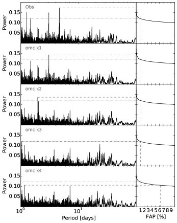
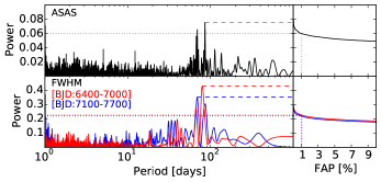
Figure 1: Periodogram analysis of the RV (top panel) and the ASAS photometry and FWHM_CCF (bottom panel). Dashed lines highlight the strongest peaks, dotted lines represent the 1% FAP threshold. Three RV signals have an FAP lower than 1%, while a fourth is just above this level of confidence. The final RV residual (omc k4) does not show any significant periodicity. The photometry and FWHM_CCF show a $\sim$83-day periodicity linked to the stellar rotation. Pre- (red) and post- (blue) fiber upgrade data are analyzed separately.

We computed the generalized Lomb-Scargle periodogram (Zechmeister & Kürster, 2009) of the RVs and residues by progressively subtracting a Keplerian fit accounting for the strongest peak in the periodogram (Fig. 1). We adjusted up to four Keplerian curves plus a velocity offset between the data obtained before and after the HARPS fibre upgrade (BJD=2457172, Lo Curto et al., 2015). The top panel in Figure 1 shows three clear periodic RV signals at 4.7, 3.1, and 2.0 days, with a false-alarm probability (FAP) ¡1/10,000. A fourth less clear signal is seen with a one-day periodicity and a 1.1% FAP. The Bayesian information criterion (BIC) for a constant model is 857.83, and for a model of one, two, three, and four Keplerian, the BIC is 463.57, 420.21, 392.62, and 376.10, respectively. On the one hand, the BIC favors the model consisting of four Keplerian curves, but on the other hand, the FAP of the fourth signal is above the 1% FAP threshold. We prefer to stay on the conservative side and consider the fourth signal as tentative. A more rigorous Bayesian model comparison and/or additional data are needed to elucidate the reliability of the one-day RV signature.

3.2 Stellar activity

YZ Cet is an active star with $log(R^{\prime}_{HK})$=-4.705$\pm$0.208. Such a $R^{\prime}_{HK}$ level translates into a rotation period of 27$\pm$9 days (Astudillo-Defru et al., 2017a). However, there are clues that flaring stars like Proxima Centauri do not follow the $log(R^{\prime}_{HK})-P_{Rot}$ relationship. This is the case for YZ Cet, where several flares are identified in spectra through Ca II HK, Na D, He I D3, and H$\alpha\beta\gamma\delta$. These chromospheric activity indicators do not show evidence of stellar rotation.

Contrary to the chromospheric activity indicators, the V-band photometry and the FWHM show evidence of the rotation period of YZ Cet ($\sim$83 days, Fig. 1). Conversely, none of the periodicities detected in the RV time series appears in the photometry or FWHM data.

3.3 Three Keplerian+Gaussian process

As the star rotates, quasi-periodic signals may be introduced in RV as a result of evolving active regions. These signals are often very complex, and a physical model is therefore usually hard to produce or has the strong disadvantage of being computationally expensive. Gaussian process regression (GP) has become a widely used non-parametric method to model this variability without the necessity of specifying a model (Rasmussen & Williams, 2006; Haywood et al., 2014; Rajpaul et al., 2015; Faria et al., 2016), although it may be prone to inducing false positives if care is not taken (Dumusque et al., 2017).

A GP with a quasi-periodic covariance function was added to the three-Keplerian model. The GP hyperparameters were sampled together with the model parameters. We set a normal prior on the recurrence timescale, $\mathcal{P}$ (see Appendix A), centered at 83 days and with a width of 15 days, in agreement with the measured stellar rotation rate (see Sect. 3.2). A detailed description of the model and the choice of priors is provided in Appendix A.

The 23-dimensional parameter space of our model was explored with the Markov chain Monte Carlo (MCMC) algorithm described in Goodman & Weare (2010) and implemented by Foreman-Mackey et al. (2013), where 100 walkers were used. The algorithm was started at a random point in the prior and was allowed to evolve until no further variation in mean posterior density across the walkers was seen. Then, the algorithm was run for a further 100,000 steps used for the inference process. We retained only those walkers that explored the main period peak for each planet (Fig 1), whose samples where used to initialize a new 70,000-step MCMC run using 300 walkers. The final inference was made on $2.1\times 10^{7}$ posterior samples, out of which over 21,000 are independent (see Appendix B for details). Results are reported in Table 5.

4 Results

4.1 Compact system near the 3:2 resonances

The periodogram and activity analysis (Sect. 3.1, 3.2) both give strong evidence that the very-low-mass star YZ Cet is orbited by at least three planets in a compact architecture. From the Keplerian modeling combined with the Gaussian processes, we obtain orbital periods of 4.66, 3.06, and 1.97 days, that is, orbits close to the 3:2 mean-motion resonances. Considering the stellar mass of 0.13M_⊙, the measured semi-amplitude translates into terrestrial-mass planets with minimum masses of 1.14, 0.98, and 0.75 Earth-masses, respectively. Table 2 gives the basic parameters of the system. Figure 2 shows the RV folded to each period.

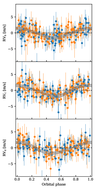
Figure 2: Radial velocities folded to each maximum a posteriori orbital period (planets b, c, and d from top to bottom, respectively). Gray shaded regions extend between the 5th and 95th percentile of the model at each orbital phase, computed over 10,000 samples of the posterior. Orange and blue circles depict data before and after the HARPS fibre upgrade, respectively.

Table 2: Basic orbital parameters of the planets. All parameters can be found in Table 5.

		YZ Cet b	YZ Cet c	YZ Cet d
M $\sin$ i	[MEarth]	$0.75\pm 0.13$	$0.98\pm 0.14$	$1.14\pm 0.17$
P	[days]	$1.96876$	$3.06008$	$4.65627$
	[days]	$\pm 0.00021$	$\pm 0.00022$	$\pm 0.00042$
e		$0.00\pm 0.12$	$0.04\pm 0.11$	$0.129\pm 0.096$
a	[au]	$0.01557$	$0.02090$	$0.02764$
	[au]	$\pm 0.00052$	$\pm 0.00070$	$\pm 0.00093$

4.2 Dynamical modeling

We show in Figure 3 a stability analysis focused on planet c where all orbital parameters are fixed to the maximum a posteriori (MAP) solution, and we varied only the semi-major axis and the eccentricity. For each set of initial conditions, we integrated the system for 1 kyr using GENGA (Grimm & Stadel, 2014), and computed the NAFF stability indicator (Laskar, 1990, 1993; Correia et al., 2005). This showed that the MAP solution is stable and outside the two 3:2 mean-motion resonances. We also see that $e_{\mathrm{c}}\lesssim 0.1$ is required for the system to remain stable.

Additionally, we used the n-body code REBOUND (Rein & Liu, 2012) with the WHFast integrator (Rein & Tamayo, 2015) to obtain the RV of the bodies in time, which we compared with the HARPS data. A stability criterion was imposed based on an additional n-body integration of 1 kyr in the future. The change in period of a planet in 1 kyr ($\Delta P_{\rm 1\leavevmode\nobreak\ kyr}$) was extrapolated to 5 Gyr (the estimated age of the system) assuming $\Delta P_{\rm 5\leavevmode\nobreak\ Gyr}\sim\Delta P_{\rm 1\leavevmode\nobreak\ kyr}\sqrt{\rm 5\leavevmode\nobreak\ Gyr/1\leavevmode\nobreak\ kyr}$. The model was rejected when $\Delta P_{\rm 5\leavevmode\nobreak\ Gyr}$ was longer than the measured orbital period, which is a conservative criterion rejecting unstable configurations. We used a normal distribution as prior for the stellar mass (Table 1) and uniform priors for the remaining parameters. The emcee algorithm (Goodman & Weare, 2010; Foreman-Mackey et al., 2013) was used to sample the posterior distribution of the parameters. We estimated the planet masses without the degeneracy with an orbital inclination relative to the line of sight by modeling the gravitational interaction between the three well-known planets in the system. From this preliminary analysis, until the fourth signal is confirmed (or rejected), we obtain M${}_{\rm b}=1.30^{+1.0}_{-0.56}$M_⊕, M${}_{\rm c}=2.1^{+1.5}_{-1.0}$M_⊕, and M${}_{\rm d}=1.74^{+1.3}_{-0.51}$M_⊕ (median and 68.3% credible interval), thanks to the constraint on the inclination: 95% HDI $i_{\rm b}$[10, 172]°, $i_{\rm c}$[6, 174]°, and $i_{\rm d}$[28, 174]°. Tighter constraints are also obtained for the eccentricities of the measured planets, $e_{\rm b}<0.39$, $e_{\rm c}<0.15$, and $e_{\rm d}<0.17$ at 95%.

5 Conclusions

We presented the discovery of three terrestrial-mass planets orbiting the very-low-mass star YZ Cet. The best fit (three Keplerian+GP) to our 13 years of HARPS data results in compact orbits close to the 3:2 mean-motion resonance with orbital periods of 1.97, 3.06, and 4.66 days. The measured minimum masses are 0.75, 0.98, and 1.14 Earth-masses, respectively, with a typical uncertainty of 16%. A fourth planet with a minimum mass of 0.42$\pm$0.11M_⊕ and an orbital period of 1.0419 days may be present in the system (1.1%FAP). To date, these are the lowest minimum masses measured through radial velocity.

From a dynamical analysis, we infer the upper limits of the planetary masses, resulting in masses below three Earth-masses. It is probable that these have radii up to 1.5R_⊕ (Fulton et al., 2017) with a rocky bulk composition. The planets orbit outside the habitable zone of YZ Cet, with equilibrium temperatures ranging from 347–491 K, 299–423 K, and 260–368 K for planets b, c, and d, respectively.

The the system is at only 3.6 pc, making it very attractive for further characterization, especially if any of the planets is caught transiting its host star, which is not the case so far.

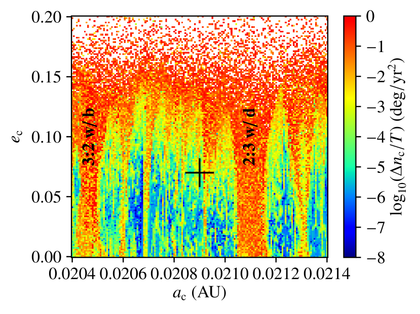
Figure 3: Stability analysis around the MAP solution (marked with a black cross, see Table 5). Blue points correspond to stable and red points to unstable solutions. White points correspond to highly unstable solutions, i.e., with a collision or the ejection of a planet during the 1 kyr of the simulation. The 3:2 resonances between planets b and c and between planets c and d are highlighted.

Appendix A Gaussian process model

A quasi-periodic kernel was chosen to construct the elements of the covariance matrix of the observations. This type of covariance function was used in the past to model the effect of stellar active regions rotating in and out of view as the star revolves (Haywood et al. 2014; Rajpaul et al. 2015).

The elements of the covariance matrix are then given by $K_{ij}=K^{r}_{ij}+K^{w}_{ij}$, where

$$K^{r}_{ij}=k_{\{A;\tau;\mathcal{P};\epsilon\}}(t_{i},t_{j})=A^{2}\exp\left[-\frac{(t_{i}-t_{j})^{2}}{2\tau^{2}}-\frac{2}{\epsilon}\sin^{2}\left(\frac{\pi(t_{i}-t_{j})}{\mathcal{P}}\right)\right]$$

represents the RV effect related to the stellar rotational modulation, with $\{A,\tau,\mathcal{P},\epsilon\}$ the hyperparameters associated with the covariance amplitude, the evolution timescale, the recurrence timescale (the rotational period of the star), and the smoothing parameter, respectively. The second term is a diagonal matrix with the quadratic sum of the internal velocity errors ($\sigma_{i}$) and an additional white-noise component:

$$K^{w}_{ij}=\left(\sigma_{i}^{2}+S_{i}\sigma_{J}^{2}+S^{+}_{i}\sigma^{+2}_{J}\right)\;\delta_{ij}\;\;,$$

where $S_{i}$ is an indicator variable that is one if observation $i$ is taken before the HARPS fibre upgrade and zero otherwise, and vice versa for $S^{+}_{i}$. $\delta_{ij}$ is the Kronecker delta function.

The prior distribution of the hyperparameters can be factorized in the marginal prior distributions described in Table 4. Only the recurrence timescale $\mathcal{P}$ was assigned an informative prior based on the analysis of the ASAS photometric measurements and the FWHM time series.

Appendix B Details on the MCMC analysis

The ensemble sampler of Goodman & Weare (2010) implemented in the emcee package (Foreman-Mackey et al. 2013) was used to sample the joint posterior distribution of the parameters and hyperparameters of the model. The priors assigned to the model parameters are listed in Tables 3 and 4.

Initially, we chose to use 100 walkers on a 23-dimensional parameter space. The starting position of each walker was randomly drawn from the prior distribution. The burn-in period took approximately 500,000 steps, and the walkers were allowed to evolve still for around 100,000 steps. An issue usually encountered when running an MCMC algorithm is that some walkers become stuck in the local maxima, in this case, related with period aliases and other features seen in the periodogram (Fig. 1). Because of this, we decided to retain only those walkers that explored the main periodogram peak for each planet. In this manner, 47 out of the 100 walkers were kept. The samples produced by these subsets of walkers were used to initialize a second MCMC run using 300 walkers, which were run for 70,000 steps. This run had a mean acceptance fraction between walkers of around 25%. The characteristic autocorrelation length was between $3\times 10^{2}$ and $1\times 10^{3}$ steps. The average autocorrelation length over walkers was shorter than 1,000 steps for all parameters. We have then more than 700 independent samples per walker, which leads to a total of around 21,000 independent samples that are used for the parameter inference.

In Table 5 we list some characteristics of the posterior distribution based on the MCMC samples. Figure 4 shows the 2D marginal distributions of a selection of model parameters.

Table 3: Prior distribution for the Keplerian curves and velocity offset between HARPS pre- and post-fibre upgrade. The priors are the same for each Keplerian, except for the period parameter. $\mathcal{U}(x_{min},x_{max})$ is the uniform distribution between $x_{min}$ and $x_{max}$.

Parameter	Prior distribution
and units	YZ Cet b	YZ Cet c	YZ Cet c
$P$ [days]	$\mathcal{U}(1.5,2.5)$	$\mathcal{U}(2.5,3.5)$	$\mathcal{U}(4.0,5.2)$
$K$ [m/s]	$\longleftarrow\mathcal{U}(0,10)\longrightarrow$
$\sqrt{e}.\sin({\omega})$	$\longleftarrow\mathcal{U}(-1,1)\longrightarrow$
$\sqrt{e}.\cos({\omega})$	$\longleftarrow\mathcal{U}(-1,1)\longrightarrow$
$\lambda_{0}$	$\longleftarrow\mathcal{U}(0,2\pi)\longrightarrow$
$e$	$\longleftarrow\mathcal{U}(0,1)\longrightarrow$
$\Delta V_{21}$ [m/s]	$\mathcal{U}(-10,10)$

Table 4: Prior distribution for the hyperparameters of the Gaussian process kernel function. $\mathcal{J}(x_{min},x_{max})$ is the Jeffreys distribution (log-flat), $\mathcal{U}(x_{min},x_{max})$ is the uniform distribution between $x_{min}$ and $x_{max}$.

Parameter	Prior distribution
A	$\mathcal{J}(10^{-4}\>\textrm{m/s},10\>\textrm{m/s})$
$\tau$	$\mathcal{J}(0.1\>\textrm{d},1000\>\textrm{d})$
$\mathcal{P}$	N(83 d, 15 d)
$\epsilon$	$\mathcal{U}(0.5,1.5)$
$\sigma_{J}$	$\mathcal{U}(0\>\textrm{m/s},10\>\textrm{m/s})$
$\sigma^{+}_{J}$	$\mathcal{U}(0\>\textrm{m/s},10\>\textrm{m/s})$

Table 5: Orbital elements using a model of three Keplerian plus a Gaussian process. Values correspond to the maximum-a-posteriori of the MCMC, with errors being the standard deviation of the MCMC samples. In the second line we report the 95% highest-density interval.

NMeas	211
$\gamma$  [m/s]	$28301.00\pm 0.30$		$\Delta V_{21}$  [m/s]	$0.01\pm 0.60$
	$[28300.37,2831.62]$			$[-1.62,0.85]$
	GP hyperparameters
$\sigma_{J}$              [m/s]	$0.13\pm 0.28$		$\sigma^{+}_{J}$              [m/s]	$0.64\pm 0.46$
	$[0.00,0.95]$			$[0.00,1.64]$
$\log_{10}(A)$       [m/s]	$0.14\pm 0.12$		$\mathcal{P}$                [d]	$79\pm 17$
	$[-0.021,0.348]$			$[51,114]$
$\log_{10}(\tau)$        [d]	$0.68\pm 0.27$		$\epsilon$	$1.02\pm 0.29$
	$[0.28,1.40]$			$[0.54,1.50]$
		YZ Cet b	YZ Cet c	YZ Cet d
$P$	[days]	$1.96876\pm 0.00021$	$3.06008\pm 0.00022$	$4.65627\pm 0.00042$
		$[1.96858,1.96934]$	$[3.05958,3.06051]$	$[4.65565,4.65740]$
$K$	[m/s]	$1.48\pm 0.25$	$1.68\pm 0.23$	$1.72\pm 0.23$
		$[0.92,1.92]$	$[1.22,2.13]$	$[1.13,2.09]$
$e$	[0..1[	$0.00\pm 0.12$	$0.04\pm 0.11$	$0.129\pm 0.096$
		$[0.00,0.41]$	$[0.00,0.37]$	$[0.000,0.311]$
$\lambda_{0}$ at BJDref=2456845.73	[deg]	$233.9\pm 9.4$	$298.8\pm 8.3$	$319.9\pm 8.8$
		$[215.0,254.2]$	$[283.5,316.4]$	$[297.8,333.4]$
$\sqrt{e}.\cos({\omega})$		$0.02\pm 0.27$	$-0.19\pm 0.21$	$-0.06\pm 0.22$
		$[-0.61,0.43]$	$[-0.48,0.32]$	$[-0.41,0.43]$
$\sqrt{e}.\sin({\omega})$		$-0.04\pm 0.26$	$-0.07\pm 0.24$	$0.36\pm 0.22$
		$[-0.47,0.56]$	$[-0.63,0.26]$	$[-0.28,0.55]$
M $\sin$ i	[MEarth]	$0.75\pm 0.13$	$0.98\pm 0.14$	$1.14\pm 0.17$
		$[0.436,0.964]$	$[0.675,1.267]$	$[0.723,1.389]$
a	[au]	$0.01557\pm 0.00052$	$0.02090\pm 0.00070$	$0.02764\pm 0.00093$
		$[0.01444,0.01661]$	$[0.01938,0.02229]$	$[0.02564,0.02948]$
Teq for AB=[0.75, 0]	[K]	[347, 491]	[299, 423]	[260, 368]
BJD${}_{\rm Trans}-2456846.0$	[days]	$0.911\pm 0.095$	$1.05\pm 0.14$	$1.44\pm 0.16$
		$[0.723,1.137]$	$[0.74,1.35]$	$[1.16,1.79]$
Trans. Prob.	[%]	5.7	4.1	2.9

Table 6: Radial velocity time series for YZ Cet (minimal; full version available at the CDS).

BJD - 2400000	RV	$\sigma_{RV}$	FWHM	Contrast	BIS	S-index	$H\alpha$
	$[kms^{-1}]$	$[kms^{-1}]$	[$kms^{-1}$]		[$kms^{-1}$]
52986.601206	28.30238	0.00411	3.88737	32.84564	-6.56400	52.61462	0.10798
52996.557553	28.29836	0.00191	3.85895	32.12375	-16.80400	5.11522	0.13170
53337.624714	28.29440	0.00126	3.83507	32.66167	-20.33000	4.52328	0.12505
53572.915467	28.30120	0.00196	3.84791	32.46511	-18.21900	5.86166	0.12981
53573.902402	28.29976	0.00271	3.85660	32.13906	-24.79800	5.77385	0.12642

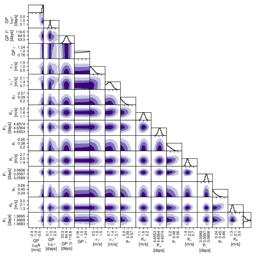
Figure 4: One- and two-dimensional marginal posterior distributions of selected model parameters. The contours represent the 68.27%, 95.45%, and 99.73% joint credible regions.