Maxwell-Hall access resistance in graphene nanopores

Abstract

The resistance due to the convergence from bulk to a constriction, for example, a nanopore, is a mainstay of transport phenomena. In classical electrical conduction, Maxwell, and later Hall for ionic conduction, predicted this access or convergence resistance to be independent of the bulk dimensions and inversely dependent on the pore radius, $a$, for a perfectly circular pore. More generally, though, this resistance is contextual, it depends on the presence of functional groups/charges and fluctuations, as well as the (effective) constriction geometry/dimensions. Addressing the context generically requires all-atom simulations, but this demands enormous resources due to the algebraically decaying nature of convergence. We develop a finite-size scaling analysis, reminiscent of the treatment of critical phenomena, that makes the convergence resistance accessible in such simulations. This analysis suggests that there is a “golden aspect ratio” for the simulation cell that yields the infinite system result with a finite system. We employ this approach to resolve the experimental and theoretical discrepancies in the radius-dependence of graphene nanopore resistance.

Ion transport through pores and channels plays an important role in physiological functions Hille (2001); Bagal et al. (2012); Rasband (2010) and in nanotechnology, with applications such as DNA sequencing Kasianowicz et al. (1996); Clarke et al. (2009); Sathe et al. (2011), imaging living cells Hansma et al. (1989); Korchev et al. (1997); Panday and He (2015), filtration Karan et al. (2015), and desalination Lee et al. (2011), among others. These pores localize the flow of ions and molecules across a membrane, where sensors, for example, nanoscale electrodes for DNA sequencing Zwolak and Di Ventra (2008, 2005); Lagerqvist et al. (2006, 2007); Krems et al. (2009); Tsutsui et al. (2010); Chang et al. (2010) , can interrogate the flowing species as they pass through and where functional elements can selectivity regulate the movement of different species (for example, ion types).

In particular, from DNA sequencing Garaj et al. (2010); Merchant et al. (2010); Schneider et al. (2010); Heerema and Dekker (2016) to filtration Joshi et al. (2014); Abraham et al. (2017); O’Hern et al. (2014); Jain et al. (2015); Surwade et al. (2015), graphene nanopores and porous membranes are one of the most promising materials for applications. Novel fabrication strategies and designs are under development to create large-scale, controllable porous membranes O’Hern et al. (2014); Jain et al. (2015); Rollings et al. (2016) and graphene laminate devices Joshi et al. (2014); Abraham et al. (2017). Moreover, their single atom thickness makes these systems ideal for interrogating ion dehydration Sahu et al. (2017); Sahu and Zwolak (2017), which both sheds light on recent experiments on ion selectivity in porous graphene O’Hern et al. (2014); Jain et al. (2015); Rollings et al. (2016) and will help analyze the behavior of biological pores Sahu et al. (2017); Sahu and Zwolak (2017). Dehydration has been predicted to give rise to ion selectivity and quantized conductance in long, narrow pores Zwolak et al. (2009, 2010); Song and Corry (2009); Richards et al. (2012a, b) but the energy barriers are typically so large that the currents are minuscule, which is rectified by the use of membranes with single-atom thickness Sahu et al. (2017); Sahu and Zwolak (2017).

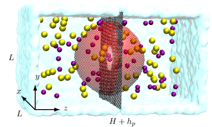
Figure 1: Schematic of a graphene nanopore. The ionic solution is partitioned by a graphene monolayer (the gray, honey-comb membrane) of thickness $h_{p}$. Potassium (purple) and chloride (yellow) ions are shown as van der Waals spheres but water is not shown even though it is explicitly present in the simulations. The remaining details are in the supplemental material (SM). The red indicates the access region. The total simulation cell is of height $H+h_{p}$ and cross section $L\times L$.

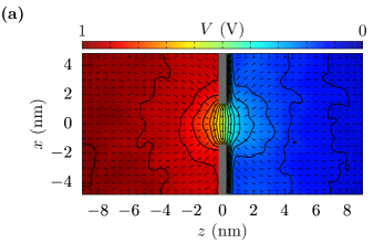
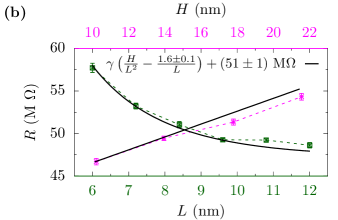
Figure 2: Electric potential and total resistance. (a) The potential $V$ (color map with contour lines at 0.05 V intervals) and normalized current density (arrows) with a 1 V applied potential and a 1.18 nm pore radius. The resistance is large in the pore region, resulting in a large electric field across the membrane [over about 1 nm]. (b) Resistance versus the cell height $H$ (magenta) and cross-sectional length $L$ (green) for the pore in (a). For $R$ versus $H$ ($L$), we use $L=9.6$ nm ($H\approx 14$ nm). Equation (9) provides a good fit to the data, yet it predicts $R_{\infty}$ is higher than where the data apparently converges. This is due to the bulk dimensions not changing in tandem as the ansatz indicates should be done. The value of $R_{\infty}$, though, is consistent with the proper scaling procedure, see Figure 4. We use the electrolyte resistivity from MD simulations of a bulk-only cell, which gives $\gamma\approx 70$ M$\Omega$ nm. Unless otherwise noted, all error bars are $\pm 1$ block standard error.

Despite the intense and broad interest in ion transport, one of its most fundamental aspects, the convergence of the bulk to the pore, is essentially not computable with all-atom molecular dynamics (MD) Yoo and Aksimentiev (2015), yet is very important for understanding in vivo operation and characteristics of ion channels Alcaraz et al. (2017). Experiments on mono- or bi-layer graphene, show a dominant $1/a$ access resistance for a pore of radius $a$ Garaj et al. (2010, 2013); Schneider et al. (2013) as expected for an atomically thin pore. Other experiments, however, seemingly yield $1/a^{2}$ behavior Schneider et al. (2010). Moreover, simulations give contradictory results, some Hu et al. (2012) with $1/a$ and others Sathe et al. (2011) $1/a^{2}$. We develop a finite-size scaling analysis for all-atom MD to extract the full resistance, both access and pore, to allow direct comparison with experimental results. Using this, we show that graphene pores, see Figure 1, have both an access and pore resistance contribution all the way to the dehydration limit.

Hall’s form of access resistance Hall (1975) is the classic result for ions to converge from bulk, far away from the pore, to the pore mouth,

$$R_{\mathrm{MH}}=\frac{\gamma}{4a},$$ (1)

where $\gamma$ is the electrolyte resistivity and $a$ is the pore radius. When taking this resistance for both sides of the membrane, it is the same form of resistance originally given by Maxwell Maxwell (1881) and later by Holm Holm (1958) and Newmann Newman (1966) for the electrical “contact” resistance of a circular orifice, which has a ballistic counterpart known as the Sharvin resistance Sharvin (1965). Maxwell’s formula for contact resistance is valid when the radius of the orifice is much larger than the mean free path of the electrons but in general the electric contact resistance is a combination of the Maxwell and Sharvin resistance Wexler (1966); Nikolić and Allen (1999).The access resistance for ion transport, however, does not have any ballistic component. We also note that the same form of access resistance is also present in thermal transport Gray and Mathews (1895); Gröber (1921) and gas diffusion Brown and Escombe (1900).

The above result assumes a hemispherical symmetry and homogeneous medium (that is, no concentration gradients, even near the pore, and no charges or dipoles on the membrane), as well as an infinite distance between the pore and electrode. These assumptions can hold for small voltages and for well-fabricated pores (for example, recent low-aspect ratio pores show only an access contribution following Eq. (1) Tsutsui et al. (2012)). Moreover, factors such as surface charges Aguilella-Arzo et al. (2005), concentration gradients Luchinsky et al. (2009); Peskoff and Bers (1988), and an asymmetrical electrolyte Läuger (1976) will influence the access resistance.

Hall’s form of access resistance is independent of bulk size, which will hold so long as the bulk dimensions are large and balanced (that is, the height of the cell should not be disproportionately large compared to its cross-sectional length). In confined geometries, however, strong boundary effects or unbalanced dimensions modify this behavior (for example, in scanning ion conductance microscopy the imposed boundary close to the pore causes the access resistance to deviate from Eq. (1) Korchev et al. (1997); Panday et al. (2016)). In MD, in particular, the simulation cells are both highly confined and periodic to collect sufficient statistical information on ion crossings. We thus examine the access resistance for a finite bulk. Its derivation is easier in rotational elliptic coordinates Maxwell (1954); Holm (1958); Newman (1966); Braunovic et al. (2006), $\xi$ and $\eta$, which are related to cylindrical coordinates, $z$ and $\rho$, via

$$z =a\xi\eta$$ (2)

$$\rho =a\sqrt{(1+\xi^{2})(1-\eta^{2})}.$$ (3)

Laplace’s equation for the potential then becomes

$$\frac{\partial}{\partial\xi}\left[(1+\xi^{2})\frac{\partial V}{\partial\xi}\right]+\frac{\partial}{\partial\eta}\left[(1-\eta^{2})\frac{\partial V}{\partial\eta}\right]=0.$$ (4)

For boundary conditions, we consider a spheroidal electrode, representing the equipotential surfaces that form even when a flat electrode is present, and a circular pore. That is, (1) $V=0$ on the pore mouth ($\xi=0$), (2) $V=V_{0}$ on a spheroidal electrode at distance $l$ ($\xi=l/a$), and (3) $\partial V/\partial\eta=0$ on the membrane surface ($\eta=0$).

Although clearly idealizations, we see features that reflect these boundary conditions from all-atom MD. Applying a constant electric field along the $z$-axis gives rise to the ion flow patterns and electric fields in Figure 2. Due to the pore resistance, a charged double layer forms Grahame (1947), with enhanced cation (anion) density on the positive (negative) voltage side. The potential at the pore mouth (which is essentially the whole pore due to the atomic thickness) is not constant, but is roughly so. The deviation is mainly due to the potassium ions coming closer to the membrane than chloride ions, pushing the potential outward. That is, the asymmetry between cations and anions (in sizes, charges, interactions), as well as other effects, distort the potential surface. The equipotential surfaces have roughly a spheroidal form (with deviation due to both simulation error, the accumulated simulation time needs to be very large, and also due to atomic-scale features of the graphene, water, and ions). Due to the large voltage and the non-zero pore resistance, only boundary condition (3) does not appear to be present. However, we expect the right functional dependence of the finite-size deviation from the Maxwell-Hall form.

Using those boundary conditions, Eq. (4) yields

$$\frac{V}{V_{0}}=\frac{\tan^{-1}\xi}{\tan^{-1}(l/a)}.$$ (5)

The ionic current through the pore is then

$$I=\frac{1}{\gamma}\int_{0}^{a}\frac{\partial V}{\partial z}\Big{|}_{z=0}\ \rho d\rho=\frac{2\pi aV_{o}}{\gamma\tan^{-1}(l/a)},$$ (6)

giving the access resistance

$$R_{\mathrm{access}} =\frac{\gamma\tan^{-1}(l/a)}{2\pi a}\approx R_{\mathrm{MH}}\left(1-\frac{2a}{\pi l}\right),$$ (7)

where the approximation is up to $\mathcal{O}\left[\frac{a}{l}\right]^{3}$ (when $l$ is about 2$a$, the higher order corrections are small, about 2.6 %, likely much smaller than corrections due to atomic details at this scale). In confined geometries, one needs to account for $a/l$ correction term, especially in MD where the computational cost typically keeps the “bulk” dimensions around 10 nm.

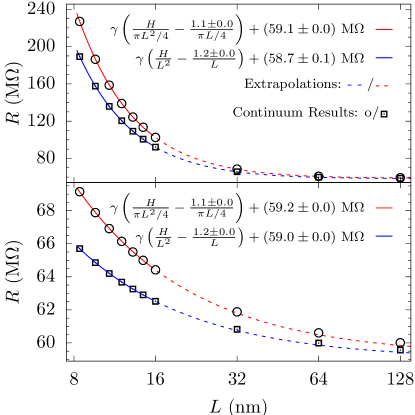
Figure 3: Pore and access resistance in continuum simulations. Resistance versus the bulk dimension $L$ for cylindrical (circles) and rectangular (squares) cells. The membrane height is 1 nm (that is, approximately that for graphene plus the charged double layer) and the pore radius is $a=1$ nm (and $\gamma$ is from MD for consistency). The bulk height is fixed to $H=140$ nm in the top panel and the aspect ratio is fixed at $H=2L$ in the bottom panel. We fit Eq. (9) for $L\leq 16$ (solid lines) and extrapolate to larger $L$ (dashed lines). The fit accurately determines $R_{\infty}$. Hence, the small simulation sizes in all-atom MD should be sufficient to obtain $R_{\infty}$.

Away from the membrane, the equipotential surfaces start to become flatter, taking on a bulk-like form. That is, the flow lines, while pointing towards the pore near its entrance/exit, orient along the $z$-axis further away, as do the electric field lines. For a simulation cross-sectional area of $A=\mathcal{G}L^{2}$, where $\mathcal{G}=\pi/4$ for a cylindrical cell and $\mathcal{G}=1$ for a rectangular cell, the access region must end by $l=f_{1}L/2$, with $f_{1}\sim\mathcal{O}(1)$, as the ellipsoidal potential surfaces encounter the cell boundary. Sometime afterward, at $f_{2}L/2$ with $f_{2}\sim\mathcal{O}(1)$, a normal bulk region appears. Thus, the total resistance is approximately

$$R= 2\left(R_{\mathrm{MH}}-\frac{\gamma}{2\pi f_{1}L/2}\right)+\frac{\gamma(H-2f_{2}L/2)}{\mathcal{G}L^{2}}+\frac{\gamma f_{3}}{\mathcal{G}L}+R_{\mathrm{pore}}.$$ (8)

The first (access-like) term occurs on both sides of the membrane (giving the factor of 2). The second (bulk-like) term uses the total height $H$ minus the two access/transitory regions of height $f_{2}L/2$ ($H$ does not include the membrane thickness and charged double layers, and it must be reasonably larger than $f_{2}L$). Figure 2(b) shows we indeed have this bulk-like region as the resistance increases linearly with $H$. The third term is a correction, $\gamma f_{3}/\mathcal{G}L$, to account for the resistance of the transition region between the access and the normal bulk, both of which would drop as $1/L$ in that finite region.

We note that some previous studies have shown the dependence of the ionic current on the cell height Gumbart et al. (2012); Jensen et al. (2013). However, in Ref. Gumbart et al., 2012, the dependence is examined in the context of changing field with the height and, in Ref. Jensen et al., 2013, the difference is considered insignificant. In linear response, the pore resistance should be independent of the applied field. While we have a 1 V potential, the main findings hold for smaller voltages, as continuum simulations demonstrate, and there is roughly linear behavior of the graphene I-V curve at this voltage Sahu et al. (2017).

Since all three corrections depend on $1/L$, we can combine them into a single term, yielding

$$R= \gamma\left(\frac{H}{\mathcal{G}L^{2}}-\frac{f}{\mathcal{G}L}\right)+R_{\infty},$$ (9)

where $R_{\infty}$ is the combined access and pore resistance when all the linear dimensions of the cell are balanced and large compare to the pore radius. The behavior of $R_{\infty}$ is expected to be $R_{\infty}=2R_{\mathrm{MH}}+R_{\mathrm{pore}}$ from Hall’s theroy, which we will show later to hold for graphene pores down to the dehydration limit. The factor $f=2\mathcal{G}/\pi f_{1}+f_{2}-f_{3}$ depends on geometric details of the cell. Assuming $f_{1}\approx f_{2}\approx 1$ (and $f_{3}$ small), $f\approx 1.6$ for a rectangular and $f\approx 1.5$ for a cylindrical cross-section. The estimates will remain close even if $f_{3}$ is substantial, so long as the transitory region is approximately a mix of access and bulk-like behavior. Despite these estimates, we treat $R_{\infty}$ and $f$ as fitting parameters.

Figure 2(b) already shows that this scaling form can capture the dependence of the resistance on the cell dimensions. However, a very peculiar behavior arises: $R_{\infty}$ is above the decay of $R$ with $L$. The scaling form, though, suggests that one should take $H=\alpha L$, where $\alpha$ is the cell aspect ratio, reducing Eq. 9 to $R=\gamma\left(\frac{\alpha-f}{\mathcal{G}L}\right)+R_{\infty}$. This indicates that if we knew $f$ exactly, we could take $\alpha=f$, that is, a “golden aspect ratio” (the estimated $f$ is not the actual golden ratio, $(1+\sqrt{5})/2$) to remove the $L$-dependence of $R$ and obtain $R=R_{\infty}$ for a finite size simulation cell. Of course, if the simulation cell is too small, the potential and densities will be artificially distorted at the periodic boundary (or finite edge). Since we do not know $f$ exactly, we will take $\alpha=2$, somewhat larger than the expected value of $f$, which will simultaneously ensure that $R$ converges to $R_{\infty}$ from above and reduce the amount that $R$ changes as $L$ increases. As well, $H$ should be reasonably larger than twice the access region, as otherwise ions would have unusual flow patterns. We prove the existence of the golden aspect ratio using continuum simulations in Ref. Sahu and Zwolak (2017).

We first examine Eq. (9) with continuum simulations, that is, using Laplace’s equation, of both rectangular and cylindrical (finite) cells using a commercial finite element solver. Figure 3 shows that continuum simulations yield good agreement with the ansatz and allow for the extrapolation of $R_{\infty}$ using small simulation cells, which bodes well for the small simulation sizes typical of all-atom MD. Moreover, it suggests that using the constant aspect ratio cells is better, as it yields less deviation over all.

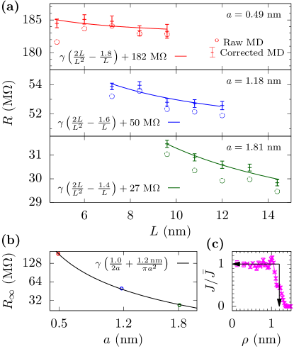
Figure 4: Pore and access resistance in graphene. (a) The three panels show the resistance versus cross-sectional length of the simulation cell for different pore sizes. The resistance from MD is shown in circles and the resistance corrected to $H=2L$ is used for fitting the model (equilibration changes $H$ from its initial value). The scaling analysis suggests the “golden aspect ratio” of $H/L\approx(1+2/\pi)$ will remove $L$ dependence of $R$. We choose an aspect ratio slightly above this so that the variation of $R$ is small but that the infinite system limit is approached from above. Unbalanced cells, for example, Figure 2(b) and Figure 3 upper panel, give much larger changes in $R$ and can also result in unusual convergence to $R_{\infty}$. (b) The extracted $R_{\infty}$ versus the pore radius $a$ indicates that there is a Maxwell-Hall access contribution. (c) Normalized current density inside a pore ($a=1.18$ nm) showing that the effective pore radius is about $0.25$ nm smaller than the geometric radius. The errors in $f$ and $R_{\infty}$ are approximately $\pm 0.1$ and $\pm 1$ M$\Omega$, respectively, for all of the pores.

We now employ our finite-size scaling ansatz to examine the total resistance in graphene nanopores. Figure 4(a) shows the resistance versus $L$ for $H=2L$. Using the extracted $R_{\infty}$, we can determine the behavior of the resistance versus $a$ (due to computational cost, we examine only a small range of $a$), see Figure 4(b). We find that even at the nanometer scale, the resistance of graphene follows the continuum form

$$R_{\infty} =2R_{\mathrm{MH}}+R_{\mathrm{pore}}=\frac{\gamma}{2a}+\frac{\gamma h_{p}}{\pi a^{2}}.$$ (10)

However, the radius can not be taken as the geometric radius (the largest circle that will fit within the pore, even correcting for van der Waals interactions). Rather, the radius is determined by the accessible area in the pore. Figure 4(c) shows how the current density in the pore tapers off as the radial coordinate increases (see also the SI). Hence, taking the pore radius from the actual effective area for current to flow accounts for hydration layers around the ions and van der Waals interactions, as well as fluctuations of the pore edge. Doing so, we find $R_{\infty}=\gamma/2a+h_{p}^{eff}\gamma/\pi a^{2}$ with $h_{p}^{eff}=(1.2\pm 0.1)$ nm. That is, we find the Maxwell-Hall access contribution and an effective thickness of 1.2 nm, in agreement with the charged double layer separation. This thickness is larger, but within the error, of the 0.6 nm value found experimentally Garaj et al. (2010); Schneider et al. (2013), where, however, the voltage was an order of magnitude smaller and thus the charge double layer was less prominent.

Thus, the resistance is a combination of both $1/a$ and $1/a^{2}$ behavior. Contextual aspects due to, e.g., van der Waals interactions, hydration layers, edge fluctuations, charge double layers, and potentially effective ion mobilities in the pore, obscure the parameters that appear in $R_{\infty}$, making it difficult to determine the dependence of the resistance on the radius. Indeed, the proper pore radius, the one related to the accessible area, is crucial. Experimentally, there are many sources of ambiguity: Uncertainties in measured values and in the pore depth (for example, multi-layer versus single layer graphene) and pore size (and aspect ratio / non-circularity), plus unknown charged functional groups or dipoles (that would enhance $1/a$ behavior by creating excess density at the membrane surface that “feeds” the current through the pore via its circumference), all affect either the balance of $1/a$ and $1/a^{2}$ behavior, or how well one can extract that behavior. This list can also include nonlinearities (for example, MD simulations show the onset of polarization-induced chaperoning of ions Sahu et al. (2017), which can tilt the balance in favor of access resistance as the dominant resistance). Different membranes and conditions can thus display diverse behavior, but “ideal” graphene membranes with pores larger than the dehydration limit have both access and pore contributions. As the pore radius increases, though, access resistance will dominate, as seen in Ref. Garaj et al., 2010. The observation of $1/a^{2}$ behavior must be due to interpretation (for example, the inclusion of multi-layer membranes in the data fitting, or the fitting itself) or to some unknown aspect of the experimental setup.

Our results demonstrate that one can capture pore and convergence resistance in reasonably sized simulations, despite the long-range nature of the access resistance. One may also extract separately the access and pore contributions to resistance, which, however, would require knowing where to partition the voltage drop (in the presence of charge double layers and other nanoscale structure, this is not a simple task). Thus, when designing porous membranes, one can use MD to both capture the “contextual” aspects of the pores, atomic scale details such as charges, fluctuations, and geometry, and the influence of the bulk electrolyte. This will allow for a quantitative comparison between measurements and simulations. Moreover, filtration and other nanopore technologies typically require many pores. The access contribution in such porous membranes is crucial, as it can undergo a transition into collective behavior when the pore density is high. Inevitably, there will be a trade off between the physical dimensions of these simulations and the time scales (and voltages) reachable. Our finite-size scaling ansatz, Eq. (9), gives a theoretical approach to guide this trade off and determine the influence of convergence.

Methods

We used NAMD2 Phillips et al. (2005) to perform all-atom molecular dynamics simulations with 2 fs integration time step and periodic boundary condition in all direction. The force field parameters is rigid TIP3P Jorgensen et al. (1983) for water and from CHARMM27 Feller and MacKerell (2000) for the rest of the atoms. Short range electrostatic and van der Waals forces have cutoff of 1.2 nm. However, full electrostatic calculation occur every 4 time steps using the Particle Mesh Ewald (PME) method.

References

- Hille (2001) B. Hille, Ion channels of excitable membranes, Vol. 507 (Sinauer Sunderland, MA, 2001).
- Bagal et al. (2012) S. K. Bagal, A. D. Brown, P. J. Cox, K. Omoto, R. M. Owen, D. C. Pryde, B. Sidders, S. E. Skerratt, E. B. Stevens, R. I. Storer, and N. A. Swain, J. Med. Chem. 56, 593 (2012).
- Rasband (2010) M. N. Rasband, Nature Education 3, 41 (2010).
- Kasianowicz et al. (1996) J. J. Kasianowicz, E. Brandin, D. Branton, and D. W. Deamer, Proc. Natl. Acad. Sci. U. S. A. 93, 13770 (1996).
- Clarke et al. (2009) J. Clarke, H.-C. Wu, L. Jayasinghe, A. Patel, S. Reid, and H. Bayley, Nat. Nanotechnol. 4, 265 (2009).
- Sathe et al. (2011) C. Sathe, X. Zou, J.-P. Leburton, and K. Schulten, ACS Nano 5, 8842 (2011).
- Hansma et al. (1989) P. K. Hansma, B. Drake, O. Marti, S. A. Gould, and C. B. Prater, Science 243, 641 (1989).
- Korchev et al. (1997) Y. E. Korchev, C. L. Bashford, M. Milovanovic, I. Vodyanoy, and M. J. Lab, Biophys. J. 73, 653 (1997).
- Panday and He (2015) N. Panday and J. He, Adv. Sci. Eng. Med. 7, 1058 (2015).
- Karan et al. (2015) S. Karan, Z. Jiang, and A. G. Livingston, Science 348, 1347 (2015).
- Lee et al. (2011) K. P. Lee, T. C. Arnot, and D. Mattia, J. Membr. Sci. 370, 1 (2011).
- Zwolak and Di Ventra (2008) M. Zwolak and M. Di Ventra, Rev. Mod. Phys. 80, 141 (2008).
- Zwolak and Di Ventra (2005) M. Zwolak and M. Di Ventra, Nano Lett. 5, 421 (2005).
- Lagerqvist et al. (2006) J. Lagerqvist, M. Zwolak, and M. DiVentra, Nano Lett. 6, 779 (2006).
- Lagerqvist et al. (2007) J. Lagerqvist, M. Zwolak, and M. Di Ventra, Phys. Rev. E 76, 013901 (2007).
- Krems et al. (2009) M. Krems, M. Zwolak, Y. V. Pershin, and M. Di Ventra, Biophys. J. 97, 1990 (2009).
- Tsutsui et al. (2010) M. Tsutsui, M. Taniguchi, K. Yokota, and T. Kawai, Nat. Nanotechnol. 5, 286 (2010).
- Chang et al. (2010) S. Chang, S. Huang, J. He, F. Liang, P. Zhang, S. Li, X. Chen, O. Sankey, and S. Lindsay, Nano Lett. 10, 1070 (2010).
- Garaj et al. (2010) S. Garaj, W. Hubbard, A. Reina, J. Kong, D. Branton, and J. Golovchenko, Nature 467, 190 (2010).
- Merchant et al. (2010) C. A. Merchant, K. Healy, M. Wanunu, V. Ray, N. Peterman, J. Bartel, M. D. Fischbein, K. Venta, Z. Luo, A. T. C. Johnson, and M. Drndić, Nano Lett. 10, 2915 (2010).
- Schneider et al. (2010) G. F. Schneider, S. W. Kowalczyk, V. E. Calado, G. Pandraud, H. W. Zandbergen, L. M. Vandersypen, and C. Dekker, Nano Lett. 10, 3163 (2010).
- Heerema and Dekker (2016) S. J. Heerema and C. Dekker, Nat. Nanotechnol. 11, 127 (2016).
- Joshi et al. (2014) R. Joshi, P. Carbone, F. Wang, V. Kravets, Y. Su, I. Grigorieva, H. Wu, A. Geim, and R. Nair, Science 343, 752 (2014).
- Abraham et al. (2017) J. Abraham, K. S. Vasu, C. D. Williams, K. Gopinadhan, Y. Su, C. T. Cherian, J. Dix, E. Prestat, S. J. Haigh, I. V. Grigorieva, A. K. Geim, and R. R. Nair, Nat. Nanotechnol. 12, 546 (2017).
- O’Hern et al. (2014) S. C. O’Hern, M. S. H. Boutilier, J.-C. Idrobo, Y. Song, J. Kong, T. Laoui, M. Atieh, and R. Karnik, Nano Lett. 14, 1234 (2014).
- Jain et al. (2015) T. Jain, B. C. Rasera, R. J. S. Guerrero, M. S. Boutilier, S. C. O’Hern, J.-C. Idrobo, and R. Karnik, Nat. Nanotechnol. 10, 1053 (2015).
- Surwade et al. (2015) S. P. Surwade, S. N. Smirnov, I. V. Vlassiouk, R. R. Unocic, G. M. Veith, S. Dai, and S. M. Mahurin, Nat. Nanotechnol. 10, 459 (2015).
- Rollings et al. (2016) R. C. Rollings, A. T. Kuan, and J. A. Golovchenko, Nat. Commun. 7, 11408 (2016).
- Sahu et al. (2017) S. Sahu, M. Di Ventra, and M. Zwolak, Nano Lett. 17, 4719 (2017).
- Sahu and Zwolak (2017) S. Sahu and M. Zwolak, Nanoscale 9, 11424 (2017).
- Zwolak et al. (2009) M. Zwolak, J. Lagerqvist, and M. Di Ventra, Phys. Rev. Lett. 103, 128102 (2009).
- Zwolak et al. (2010) M. Zwolak, J. Wilson, and M. Di Ventra, J. Phys.: Condens. Matter 22, 454126 (2010).
- Song and Corry (2009) C. Song and B. Corry, J. Phys. Chem. B 113, 7642 (2009).
- Richards et al. (2012a) L. A. Richards, A. I. Schäfer, B. S. Richards, and B. Corry, Small 8, 1701 (2012a).
- Richards et al. (2012b) L. A. Richards, A. I. Schäfer, B. S. Richards, and B. Corry, Phys. Chem. Chem. Phys. 14, 11633 (2012b).
- Yoo and Aksimentiev (2015) J. Yoo and A. Aksimentiev, J Phys Chem Lett 6, 4680 (2015).
- Alcaraz et al. (2017) A. Alcaraz, M. L. López, M. Queralt-Martín, and V. M. Aguilella, ACS Nano 11, 10392 (2017).
- Garaj et al. (2013) S. Garaj, S. Liu, J. A. Golovchenko, and D. Branton, Proc. Natl. Acad. Sci. 110, 12192 (2013).
- Schneider et al. (2013) G. F. Schneider, Q. Xu, S. Hage, S. Luik, J. N. Spoor, S. Malladi, H. Zandbergen, and C. Dekker, Nat. Commun. 4, 2619 (2013).
- Hu et al. (2012) G. Hu, M. Mao, and S. Ghosal, Nanotechnology 23, 395501 (2012).
- Hall (1975) J. E. Hall, J. Gen. Physiol. 66, 531 (1975).
- Maxwell (1881) J. C. Maxwell, A treatise on electricity and magnetism, Vol. 1 (Clarendon press, 1881).
- Holm (1958) R. Holm, The contact resistance. General theory (Springer, 1958).
- Newman (1966) J. Newman, J. Electrochem. Soc. 113, 501 (1966).
- Sharvin (1965) Y. V. Sharvin, Sov. Phys. JETP 21, 655 (1965).
- Wexler (1966) G. Wexler, Proc. Phys. Soc. 89, 927 (1966).
- Nikolić and Allen (1999) B. Nikolić and P. B. Allen, Phys. Rev. B 60, 3963 (1999).
- Gray and Mathews (1895) A. Gray and G. B. Mathews, A treatise on Bessel functions and their applications to physics (Macmillan and Company, 1895).
- Gröber (1921) H. Gröber, Die Grundgesetze der Wärmeleitung und des Wärmeüberganges: ein Lehrbuch für Praxis und technische Forschung (Springer-Verlag, Berlin, 1921).
- Brown and Escombe (1900) H. T. Brown and F. Escombe, Proc. Roy. Soc. London 67, 124 (1900).
- Tsutsui et al. (2012) M. Tsutsui, S. Hongo, Y. He, M. Taniguchi, N. Gemma, and T. Kawai, ACS Nano 6, 3499 (2012).
- Aguilella-Arzo et al. (2005) M. Aguilella-Arzo, V. M. Aguilella, and R. S. Eisenberg, Eur. Biophys. J. 34, 314 (2005).
- Luchinsky et al. (2009) D. Luchinsky, R. Tindjong, I. Kaufman, P. McClintock, and R. Eisenberg, Phys. Rev. E 80, 021925 (2009).
- Peskoff and Bers (1988) A. Peskoff and D. Bers, Biophys. J. 53, 863 (1988).
- Läuger (1976) P. Läuger, Biochim. Biophys. Acta 455, 493 (1976).
- Panday et al. (2016) N. Panday, G. Qian, X. Wang, S. Chang, P. Pandey, and J. He, ACS Nano 10, 11237 (2016).
- Maxwell (1954) J. C. Maxwell, A treatise on electricity and magnetism, Vol. 1 (Dover Publications, 1954).
- Braunovic et al. (2006) M. Braunovic, N. K. Myshkin, and V. V. Konchits, Electrical contacts: Fundamentals, applications and technology (CRC press, 2006).
- Grahame (1947) D. C. Grahame, Chem. Rev. 41, 441 (1947).
- Gumbart et al. (2012) J. Gumbart, F. Khalili-Araghi, M. Sotomayor, and B. Roux, Biochim. Biophys. Acta - Biomembranes 1818, 294 (2012).
- Jensen et al. (2013) M. Ø. Jensen, V. Jogini, M. P. Eastwood, and D. E. Shaw, J. Gen. Phsiol. 141, 619 (2013).
- Sahu and Zwolak (2017) S. Sahu and M. Zwolak, arXiv:1711.00472 (2017).
- Phillips et al. (2005) J. C. Phillips, R. Braun, W. Wang, J. Gumbart, E. Tajkhorshid, E. Villa, C. Chipot, R. D. Skeel, L. Kale, and K. Schulten, J. Comput. Chem. 26, 1781 (2005).
- Jorgensen et al. (1983) W. L. Jorgensen, J. Chandrasekhar, J. D. Madura, R. W. Impey, and M. L. Klein, J. Chem. Phys. 79, 926 (1983).
- Feller and MacKerell (2000) S. E. Feller and A. D. MacKerell, J. Phys. Chem. B 104, 7510 (2000).