Morphological estimators on Sunyaev–Zel’dovich maps of MUSIC clusters of galaxies

Abstract

The determination of the morphology of galaxy clusters has important repercussion on their cosmological and astrophysical studies. In this paper we address the morphological characterisation of synthetic maps of the Sunyaev–Zel’dovich (SZ) effect produced for a sample of 258 massive clusters ($M_{vir}>5\times 10^{14}h^{-1}$M_⊙ at $z=0$), extracted from the MUSIC hydrodynamical simulations. Specifically, we apply five known morphological parameters, already used in X-ray, two newly introduced ones, and we combine them together in a single parameter. We analyse two sets of simulations obtained with different prescriptions of the gas physics (non radiative and with cooling, star formation and stellar feedback) at four redshifts between 0.43 and 0.82. For each parameter we test its stability and efficiency to discriminate the true cluster dynamical state, measured by theoretical indicators. The combined parameter discriminates more efficiently relaxed and disturbed clusters. This parameter had a mild correlation with the hydrostatic mass ($\sim 0.3$) and a strong correlation ($\sim 0.8$) with the offset between the SZ centroid and the cluster centre of mass. The latter quantity results as the most accessible and efficient indicator of the dynamical state for SZ studies.

1 Introduction

Clusters of galaxies are the largest virialized objects in the universe and they play a key role in the understanding of the formation, the growth, and the properties of large-scale structures. The investigation of cluster dynamical state has important astrophysical and cosmological implications. The disturbed nature of a cluster can be in fact the indicator of violent mergers. A sample of disturbed clusters would allow to characterize the motions arising from these events, which are of crucial importance for an accurate estimate of the non-thermal pressure support which will need to be constrained to enable accurate cluster cosmology (see e.g. Haiman et al., 2001; Borgani, 2008; Mantz et al., 2010). As shown from numerical simulations, values of cluster masses derived only from the assumption of hydrostatic equilibrium, and thus accounting only for the contribution from thermal pressure, can be significantly understimated (up to $\sim 30$ per cent) (see e.g. Lau et al., 2009; Rasia et al., 2012; Biffi et al., 2016, and references therein). Such mass bias is reduced to 10 per cent in relaxed clusters. This is one of the main reasons of the common choice to calibrate the self-similar scaling relations (see e.g. Giodini et al., 2013, for a review) towards regular objects (see e.g. Johnston et al., 2007; George et al., 2012; Czakon et al., 2015).

Historically, the very first attempts to determine whether a galaxy cluster was dynamically relaxed or not, were made through the visual inspection of the galaxy distribution in optical images (Conselice, 2003) and the regularity of the intra-cluster medium (ICM) in X-ray maps (Ulmer & Cruddace, 1982). The presence of bimodal or clumpy surface brightness distribution was considered an indication for the presence of sub-structures in dynamically active clusters (Fabian, 1992; Slezak et al., 1994; Gómez et al., 1997; Rizza et al., 1998; Richstone et al., 1992), although some exceptions have been reported (e.g. Pinkney et al., 1996; Buote & Tsai, 1996; Plionis, 2002). On the other hand, regular and mostly circular shapes of the projected gas distribution are characteristic of dynamically relaxed clusters, which have limited turbulent motions. From these early studies, several other morphological parameters have been introduced in the literature over the years (see section 3.2), and more recent applications to X-ray maps can be found in Mantz et al. (2015); Nurgaliev et al. (2017); Andrade-Santos et al. (2017) and Lovisari et al. (2017).

No morphological evaluation has been so far drawn from Sunyaev–Zel’dovich (SZ) maps observed in the millimetric band. The SZ effect (Sunyaev & Zeldovich, 1970, 1972) is produced by the Comptonization of the cosmic microwave background (CMB) photons from the interaction with the energetic free electrons in the ICM and causes a redistribution of the energy of the CMB photons. This is observed as a variation on the CMB background whose intensity depends on the observed frequency. The CMB intensity variation is proportional to the integral of the electronic thermal pressure of the ICM along the line of sight (see e.g. Carlstrom et al., 2002, for a review). Therefore the SZ effect is linearly proportional to the electron number density. For this property, the SZ effect is a fundamental complementary tool to X-ray, since it probes more efficiently the outermost regions of galaxy clusters (see e.g. Roncarelli et al., 2013). Nowadays, hundreds or even thousands of galaxy clusters observed through the SZ effect are available thanks to different surveys carried out either by ground-based facilities , as in the case of the South Pole Telescope (Chang et al., 2009; Staniszewski et al., 2009; Bleem et al., 2015) or the Atacama Cosmology Telescope (Swetz et al., 2011; Hasselfield et al., 2013), or space-based as in the case of the Planck satellite (Planck Collaboration et al., 2011, 2014, 2016). Clusters detected through the SZ effect do not show significant bias in terms of relaxation state. For instance, Rossetti et al. (2016) shows that clusters detected by Planck – whose morphology is determined through the projected offset between the peak of the X-ray emission and the position of the brightest cluster galaxy (BCG) – are equally distributed between regular and disturbed objects. On the contrary, in X-ray surveys the percentage of relaxed objects is $\approx 74$ per cent. This comparison suggests that the observational selection effects can seriously influence the result. Hence, the importance of evaluating morphology from SZ catalogues that are roughly mass-limited.

To infer cluster morphology from SZ maps one would require high sensitivity and high angular resolution. At present there are no SZ cluster catalogues with such characteristics. However, the situation might change in the coming years. Instruments like the currently operating MUSIC camera (Sayers et al., 2010) or MUSTANG-2 (Young et al., 2012), having maximum angular resolutions of $\approx 30$ and $\approx 10$ arcsec, respectively, are examples of microwave detectors aimed at producing high-resolution cluster imaging through the SZ effect. Very promising results have also been recently reported with the 30-m telescope at the IRAM observatory using the NIKA (Monfardini et al., 2010) and NIKA2 (Calvo et al., 2016; Adam et al., 2018) cameras, where the maps reach an angular resolution of $\approx 20$ arcsec (Adam et al., 2014; Mayet et al., 2017; Ruppin et al., 2017). Even better resolutions have been achieved at low frequencies with the use of interferometers, as shown in Kitayama et al. (2016). Indeed, they report the SZ imaging of a galaxy cluster at 5 arcsec from observations with the Atacama Large Millimeter Array (Booth, 2000). Since SZ maps correspond to maps of the distribution of the thermal pressure, they are extremely valuable for the investigation of cluster morphology (see Wen & Han, 2013; Cui et al., 2017, e.g.). For instance, in Prokhorov et al. (2011) they highlight the effects produced by a violent merger on the SZ imaging of a bullet-like simulated cluster, namely the presence of a cold substructure. Morphology has some impact also on the scaling relation between the integrated SZ signal and the cluster mass, as shown for simulated clusters (e.g. in da Silva et al., 2001; McCarthy et al., 2003; Shaw et al., 2008). For instance, Rumsey et al. (2016) state that mergers induce small deviations from the canonical self-similar predictions in SZ and X-ray scaling relations, in agreement with Poole et al. (2007).

Apart from these examples, there is not yet a detailed study on the morphology derived from observed or simulated SZ maps, or on the relation between SZ morphology and the cluster dynamical state. The aims of this paper are therefore: (1) to verify the feasibility of the application of some morphological parameters typically used in X-ray on SZ maps,; (2) to determine their effectiveness in segregating the cluster dynamical state (which in the case of simulated clusters is known a priori) and (3) to evaluate their possible correlation with other relevant measures such as the hydrostatic mass bias or the X-ray morphological parameters. For these goals, we use both existing and new parameters and we also combine them to derive a global parameter.

The paper is organized as follows. In section 2 we briefly describe the simulations and the data used in this analysis. In section 3 we define the criteria used in the simulation to discriminate the dynamical state, and provide a summary of the morphological parameters. The efficiency and the stability of these parameters is tested in section 4, together with a comparison between their application to X-ray and SZ maps. Finally, the correlation of the morphological indicators with the hydrostatic mass bias and with the projected shift between the centre of mass (CM) and the centroid of the SZ map is investigated in sections 5 and 6. We summarize our results and outline our conclusions in section 7.

2 Data set

The analysis presented in this work is performed on simulated clusters taken from the Marenostrum-MultiDark SImulations of galaxy Clusters (MUSIC) (Sembolini et al., 2013). The MUSIC project consists in two distinct sub-sets of re-simulated galaxy groups and clusters: MUSIC-1, which is build on objects extracted from the MareNostrum simulation (Gottlöber & Yepes, 2007); MUSIC-2, that is build on systems selected within the MultiDark simulations (Prada et al., 2012). The resimulations of all clusters are based on the initial conditions generated by the zooming technique of Klypin et al. (2001) and cover a spherical region centred on the redshift zero cluster with a radius of $6h^{-1}$Mpc. The Lagrangian regions are resimulated with the inclusion of the baryonic physics and at higher resolution. The re-simulations are carried out using the TreePM+SPH Gadget-2 code and include two different prescriptions for the gas physics. The simplest follows the evolution of a non-radiative gas, while the other includes several physical processes, such as cooling, UV photo-ionisation, stellar formation, and thermal and kinetic feedback processes associated to supernovae explosions (see details in Sembolini et al., 2013). We will refer to them as the NR and the CSF sub-sets, respectively. The final resolution is $m_{\textup{DM}}=9\times 10^{8}h^{-1}$ M_⊙ for the dark matter, and $m_{\textup{gas}}=1.9\times 10^{8}h^{-1}$ M_⊙ for the initial gas elements.

In this work we use a sample of 258 massive clusters, having virial mass $M_{vir}>5\times 10^{14}h^{-1}$M_⊙ at $z=0$, extracted from the MUSIC-2 data-set. We analyse clusters simulated with both ICM versions, and considered at four different times of their cosmic evolution, namely at redshifts $z=$ 0.43, 0.54, 0.67 and 0.82. The underlying cosmological model is that of the MultiDark parent simulation and it adopts the best-fit parameters from WMAP7+BAO+SNI: $\Omega_{m}=0.27$, $\Omega_{b}=0.0469$, $\Omega_{\Lambda}=0.73$, $\sigma_{8}=0.82$, $n=0.95$ and $h=0.7$ (see Komatsu et al., 2011). This sample has been extensively analysed in the past, with focus on the baryon and SZ properties (Sembolini et al., 2013), on the X-ray scaling relations (Biffi et al., 2014), and on motions of both dark matter and gas (Baldi et al., 2017).

2.1 Sunyaev–Zel’dovich maps and X-ray data

The SZ effect can be separated into two components: the thermal component, produced by the random motion of the electrons in the ICM, and the kinetic component, generated by the overall bulk motion of the cluster with respect to the CMB rest frame (see e.g. Carlstrom et al., 2002). In this work we focus only on the former. This produces a shift of the CMB brightness, $I_{\textup{CMB}}$:

$$\frac{\Delta I}{I_{\textup{CMB}}}=\frac{x^{4}e^{x}}{(e^{x}-1)^{2}}\left[x\coth\left(\frac{x}{2}\right)-4\right]\ y$$ (1)

where $x=h_{P}\nu/(k_{B}T_{\textup{CMB}})$, and $\nu$ is the frequency of the radiation, $h_{P}$ is the Planck constant, $k_{B}$ is the Boltzmann constant, and $T_{\textup{CMB}}$ is the CMB temperature. The $y$ factor in equation (1) is the Compton parameter, defined as:

$$y=\frac{\sigma_{T}k_{B}}{m_{e}c^{2}}\int n_{e}T_{e}d\ell$$ (2)

where $\sigma_{T}$ is the Thomson cross section, $m_{e}c^{2}$ is the electron rest mass, $n_{e}$ is the electron number density, $T_{e}$ is the electron temperature, and the integration is performed over the line of sight. In order to produce maps of the Compton parameter of our simulated clusters we refer to the discretized version of the formula, proposed in Flores-Cacho et al. (2009):

$$y\simeq\frac{\sigma_{T}k_{B}}{m_{e}c^{2}}\sum_{i}\ W_{p}\left(|\boldsymbol{r}_{i}-\boldsymbol{r}_{cm}|,h_{s}\right)n_{e,i}\ T_{e,i}\ \Delta\ell\ ,$$ (3)

where the $W_{P}$ function is the projected normalized spherical spline kernel of the simulation, i.e. the kernel presented in Monaghan & Lattanzio (1985). The kernel depends on the SPH smoothing length $h_{s}$ and is evaluated at the radial distance of the $i$-th particle with respect to the cluster centre of mass, $|\boldsymbol{r}_{i}-\boldsymbol{r}_{cm}|$. The sum in equation (3) extends to all gas particles located along the line of sight up to a maximum distance of $1.5R_{vir}$ from the cluster centre, being $R_{vir}$ the virial radius. The side of the maps has a physical size of 10 Mpc, corresponding to $\sim$ 3.4 times the mean virial radius of the sample. This extension is comparable with the maximum radius that can be probed with SZ measurements of large clusters, which e.g. for Planck is of the order of a few virial radii (Planck Collaboration et al., 2013). Each pixel is equivalent to 10 kpc. In angular distances, given the cosmological parameters adopted in the simulation, the field of view and the pixel resolution correspond to (29.6, 26.1, 23.6, 21.8) arcmin and (1.8, 1.6, 1.4, 1.3) arcsec at the four redshifts ($z=0.43,0.54,0.67,0.82$), respectively. Such large fields of view could be covered with large mosaics of detectors and multiple observational runs. For example, one would need 4 to 9 pointings with the MUSIC camera, which has a field of view of $\approx 10$ arcmin. The angular resolution of our maps, instead, is not achievable by any current instrument, that at best reaches 5 arcsec for interferometric measurements (e.g. with ALMA), and about 20 arcsec for single-dish measurements (e.g. with the NIKA2 camera). In section 4.4, we will degenerate the SZ signal to reproduce the angular resolution of three examples of existing telescopes for microwave astronomy, having diameters of 1.5, 10 and 30 m, respectively. In this work we do not consider specific observational features such the instrumental noise or any contamination with astrophysical origins. These will be properly taken into account in a forthcoming work which will address the capabilities of a specific experiment. The noise, indeed, typically shows a significant pixel-to-pixel correlation, and it is an intrinsic characteristic of the instrument. Astrophysical sources of contamination also depend on the instrument, in particular on the observed frequencies. In this study we refer to noiseless and maps without any contamination to be as general as possible.

In section 4.1.1 we compare the morphological parameters derived from SZ with those obtained from X-ray data. We use two sub-samples of the non-radiative clusters that have been selected in Meneghetti et al. (2014) to morphologically match the CLASH sample observed by Chandra and XMM-Newton in X-ray (Postman et al., 2012). These sub-samples are constituted by 79 clusters at $z=0.43$ and 86 clusters at $z=0.67$. Their X-ray maps were produced using the X-MAS software package (see Gardini et al., 2004; Rasia et al., 2008) to mimic ACIS-S3 Chandra observations, with a field of view of 8.3 arcmin and angular resolution of 0.5 arcsec.

3 Determination of the dynamical state

Before presenting the morphological parameters, we introduce the indicators of the cluster dynamical state that, in simulations, can be measured in a quantitative way from several estimators. For instance, one of the most used indicators in the literature is the ratio between the kinetic energy, $T$, and the potential energy, $W$, of the system measured within the virial radius. The ratio is expressed as $(2T-E_{S})/|W|$, where $E_{S}$ is the surface pressure energy evaluated at the same virial radius. The cluster is considered relaxed when the ratio is lower than 1.35 (see e.g. Neto et al., 2007; Ludlow et al., 2012). Even if broadly adopted, in this paper we prefer to avoid its usage since several works showed that it is often unreliable (see e.g. Sembolini et al., 2014; Klypin et al., 2016). Another criterion is based on the ratio of the gas velocity dispersion, $\sigma$, over the theoretical velocity dispersion, $\sigma_{t}$ (Cui et al., 2017). This indicator, often expressed as $\zeta=\sigma/\sigma_{t}$, could be applied to optical data, but it is still not clear whether the threshold that discriminates between relaxed and disturbed objects is mass dependent.

3.1 Indicators of the dynamical state

In this work, the cluster dynamical state is quantified through the following two parameters, derived from the 3D information of the simulated cluster. For this reason, we also called them 3D indicators:

• the ratio between the mass of the biggest sub-structure and the cluster mass evaluated within the virial radius $M_{sub}/M_{vir}$. Some variants of this parameter exist, including the ratio between the mass of all substructures and the total cluster mass (see e.g. Biffi et al., 2016; Meneghetti et al., 2014), however, we refer to its simplest definition, as e.g. in Sembolini et al. (2014);

• the offset $\Delta_{r}$ between the position of the peak of the density distribution, $\mathbf{r}_{\delta}$, and the position of the centre of mass of the cluster, $\mathbf{r}_{cm}$, normalized to the virial radius $R_{vir}$:

  $$\Delta_{r}=\frac{|\mathbf{r}_{\delta}-\mathbf{r}_{cm}|}{R_{vir}}\ .$$ (4)

We classify the cluster as relaxed if both indicators are simultaneously smaller than a certain threshold, that we fix equal to 0.1 in both cases. In literature, different thresholds are adopted for DM only simulations (see e.g. Macciò et al., 2007; D’Onghia & Navarro, 2007). In particular, for the offset parameter, it is often used a smaller value for the thresold. However, we prefer to increase it to 0.1 to accomodate the effect of baryons that reduce the displacement due their collisional nature. The fraction of relaxed and disturbed clusters is shown in Table 1, for all the analysed data sets. No significant dependence on redshift or ICM physics is seen in our data. Our sample has about 55 percent of relaxed objects.

Table 1: Percentages of clusters classified as relaxed or disturbed for the four considered redshifts and the two ICM physics.

$z$	CSF		NR
	relaxed	disturbed	relaxed	disturbed
0.43	56%	44%	55%	45%
0.54	53%	47%	53%	47%
0.67	56%	44%	55%	45%
0.82	54%	46%	53%	47%

3.2 Morphological parameters

In the following we describe the morphological parameters analysed in this work: the asymmetry parameter, the fluctuation parameter, the light concentration parameter, the third-order power ratio parameter, the centroid shift parameter, the strip parameter, the Gaussian fit parameter and a combined parameter. The first five indicators are taken from X-ray morphological studies, while we introduce here the remaining parameters. Here, we will discuss their expected behaviour in the case of relaxed or disturbed clusters.

All the parameters refer to the centroid of the analysed SZ map as center and we computed them inside different values of the aperture radius, $R_{ap}$, equivalent to 0.25, 0.50, 0.75 and 1.00 times $R_{vir}$. We will discuss which aperture works best for each parameter (see section 4).

Asymmetry parameter, $A_{\theta}$

This parameter, originally introduced by Schade et al. (1995), is based on the normalized difference between the original SZ map, $I$, and the rotated map, $R_{\theta}$, being $\theta$ the rotation angle:

$$A_{\theta}=\frac{\sum\limits_{r<R_{ap}}|I-R_{\theta}|}{\sum\limits_{r<R_{ap}}I}\ ,$$ (5)

where the sums are extended to all pixels within $R_{ap}$. We computed four different versions of this parameter, $A_{x}$, $A_{y}$, $A_{\pi}$, and $A_{\pi/2}$. For $A_{x}$ and $A_{y}$ we consider as $R_{\theta}$ the flipped image along the $x$ or the $y$ axes, respectively (as in Rasia et al., 2013). Low values of $A_{\theta}$ indicates relaxed clusters. With the purpose of making a final classification, we use the rotation angle corresponding to the maximum value of $A_{\theta}$.

Fluctuation parameter, $F$

The fluctuation parameter, introduced in Conselice (2003), is defined similarly to the asymmetry parameter. Namely, it is expressed as the normalized difference between an original image, $I$, and its Gaussian-smoothed version, $B$:

$$F=\frac{\sum\limits_{r<R_{ap}}|I-B|}{\sum\limits_{r<R_{ap}}I}\ .$$ (6)

Various versions of this parameter exist: negative residuals are ignored in Conselice (2003), or the absolute value are not considered in Okabe et al. (2010), or different values for the full-width-half-maximum (FWHM) Gaussian filter are used. We keep the absolute values to account both negative and positive residuals. Furthermore, we consider 10 equally-spaced FWHM values, from 0.05$R_{vir}$ to 0.5$R_{vir}$ to evaluate the most effective choice. Regular clusters are expected to present low values for the fluctuation parameter.

Light concentration parameter, $c$

This parameter was introduced by Santos et al. (2008) with the purpose of segregating cool core and non-cool core clusters (see also Cassano et al., 2010; Rasia et al., 2013). These analyses, based on X-ray maps, reach at best $R_{500}$ (and only in few cases they go beyond). Here we use a more general mathematical formula given by the ratio of the surface brightness computed within a radius $r_{2}$ and the one evaluated within a more central region of radius $r_{1}<r_{2}$:

$$c=\frac{\int_{0}^{r_{1}}S(r)dr}{\int_{0}^{r_{2}}S(r)dr}\ .$$ (7)

We choose the inner and outer radii as fractions of the virial radius, in order to avoid any dependence on redshift when assuming a fixed physical aperture (as discussed in Hallman & Jeltema, 2011) as it was done in Santos et al. (2008) . In particular, we set $r_{2}=R_{ap}$, and we use ten different values of $r_{1}$, uniformly sampled between 0.1 and 1.0 times $r_{2}$. We expect higher values of $c$ for relaxed clusters, since in this case the surface brightness is peaked near the cluster centre, and lower values for disturbed ones, due to their irregular shape and the possible presence of structures located far from the centre.

Third-order power ratio parameter, $P_{3}/P_{0}$

The first definition of the m-$th$ order power ratio, $P_{m}/P_{0}$, was given by Buote & Tsai (1995):

$$\frac{P_{m}}{P_{0}}=\frac{a_{m}^{2}+b_{m}^{2}}{2m^{2}R^{2}_{ap}a_{0}\ln(R_{ap})}\ ,$$ (8)

where the coefficients $a_{m}$ and $b_{m}$ are, respectively, defined as:

$$a_{m}(R_{ap})=\int\limits_{r\leq R_{ap}}S(r,\phi)r^{m}\cos(m\phi)drd\phi\ ,$$ (9)

$$b_{m}(R_{ap})=\int\limits_{r\leq R_{ap}}S(r,\phi)r^{m}\sin(m\phi)drd\phi\ ,$$ (10)

and $S(r,\phi)$ is the surface brightness expressed as a function of the projected radius and azimuthal angle, $\phi$. Following this definition, we compute the third-order power ratio $P_{3}/P_{0}$ considering $m=3$, and we take its decimal logarithm. This parameter is one among the most efficient in X-ray (see e.g. Rasia et al., 2013; Lovisari et al., 2017). We measure $P_{3}/P_{0}$ using four different aperture radii, expressed as fractions of the virial radius, and then consider its maximum value to better identify clusters with sub-structures or irregular shape which are associated to high values of the power ratio.

Centroid shift parameter, $w$

The centroid shift parameter is a measure of how much the centroid of the map with different circular sub-apertures changes. Once the centroid within $R_{ap}$ is computed, a new aperture radius is defined and the respective centroid is found. The operation is repeated for $N$ sub-apertures. The centroid shift is then defined as the normalized standard deviation of all $\Delta_{i}$ separations:

$$w=\frac{1}{R_{ap}}\sqrt{\frac{\sum(\Delta_{i}-<\Delta_{i}>)^{2}}{N-1}}$$ (11)

where $<\Delta_{i}>$ is their mean value. This parameter has been largely applied on X-ray maps in several works, altough some variations in its definition were considered. Generally it was found to be an efficient parameter to discriminate the cluster dynamical state (see e.g. Mohr et al., 1993; O’Hara et al., 2006; Poole et al., 2006; Maughan et al., 2008; Ventimiglia et al., 2008; Jeltema et al., 2008; Böhringer et al., 2010; Weißmann et al., 2013). The presence of a substructure will increase the value of the centroid shift, therefore we expect low values for relaxed clusters. Even though, this might not be the case in the presence of symmetric substructures that would be unidentified by $w$.

Strip parameter, $S$

We call “strip” a profile extracted from the SZ map and passing through its centroid. The strip parameter is the sum of the pixel-to-pixel difference between couples of different strips, $S_{i}$ and $S_{j}$, at $N$ total different angles in absolute value. In order to obtain a value of $S$ between 0 and 1, this sum is normalised by the maximum strip integral and by the number of the strip pairs considered:

$$S=\frac{\sum_{\begin{subarray}{c}i,j\\ j<i\end{subarray}}|S_{i}(r)-S_{j}(r)|}{\frac{N(N-1)}{2}\max[\int\limits_{R_{ap}}S_{i}(r)dr]}\ .$$ (12)

As usual, $R_{ap}$ indicates the aperture radius, i.e. the maximum radius within which the integration of the strips is performed. The main advantage of using this parameter is the possibility to use many non-repeated combinations of strips. Indeed, in this way the parameter quantifies the different contributions to the overall symmetry of the cluster SZ map coming from multiple angles. In our case, performing a single rotation of the SZ maps, we take four strips selected with angles equal to 0^∘, 45^∘, 90^∘ and 135^∘, for a total of six computed differences. We have tested the effects of using $N>4$ angles, finding that the dynamic range of this parameter is slightly reduced with increasing number of strips. Nevertheless, the overlap between the populations of relaxed and disturbed objects remains substantially unchanged, allowing us to choose a small number of strips to reduce the computational time without significantly affecting the final results. Disturbed clusters are expected to show higher values of the parameter because of the presence of sub-structures (visible as off-centre peaks in the strips) or possible asymmetries.

Gaussian fit parameter, $G$

The Gaussian fit parameter, $G$, is based on a two-dimensional Gaussian fitting of the SZ maps applied within the aperture radius. The Gaussian model used can be written in terms of the $x$ and $y$ coordinates as:

$$\begin{split}&f(x,y)=z_{0}+\\ &A\exp\left\{-\left[a\left(x-x_{0}\right)^{2}+2b\left(x-x_{0}\right)\left(y-y_{0}\right)^{2}+c\left(y-y_{0}\right)\right]\right\}\ ,\end{split}$$ (13)

where $a$, $b$ and $c$ are constants defined as:

$$\begin{split}&a=\frac{\cos^{2}\theta}{2\sigma_{x}^{2}}+\frac{\sin^{2}\theta}{2\sigma_{y}^{2}}\\ &b=-\frac{\sin 2\theta}{4\sigma_{x}^{2}}+\frac{\sin 2\theta}{4\sigma_{y}^{2}}\\ &c=\frac{\sin^{2}\theta}{2\sigma_{x}^{2}}+\frac{\cos^{2}\theta}{2\sigma_{y}^{2}}\ .\end{split}$$ (14)

The best-fitting parameters obtained from the procedure are the following: the angle $\theta$ between the axes of the map and those of the bi-dimensional Gaussian distribution; the coordinates of the peak of the model map, $x_{0}$ and $y_{0}$; its amplitude $A$; the offset $z_{0}$ and the two standard deviations, $\sigma_{x}$ and $\sigma_{y}$. The $G$ parameter is just defined as the ratio:

$$G=\frac{\sigma_{min}}{\sigma_{max}},$$ (15)

where $\sigma_{min}$ ($\sigma_{max}$) denotes the smallest (largest) value between $\sigma_{x}$ and $\sigma_{y}$ We expect lower values of $G$ for disturbed clusters, which should show asymmetric shapes, resulting in significantly different standard deviations along the $x$ and $y$ direction in the Gaussian fit. Instead, $G$ should be close to $1$ for regular clusters. It should be stressed that, similarly to the case of the centroid shift, this parameter could lead to a misclassification of disturbed clusters in presence of symmetrically distributed sub-structures. It should also be noted that the aperture radius within which the fit is computed should be sufficiently large, in order to take into account the presence of possible sub-structures located far from the centre.

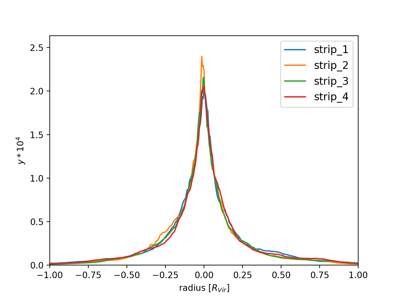
(a)

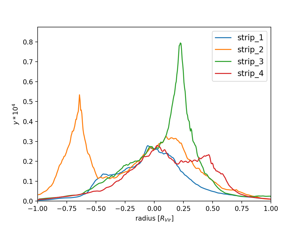
(b)

Figure 1: Strips passing through the centroid of the SZ maps of a relaxed cluster (#7, left panel) and of an unrelaxed one (#27, right panel) for the four chosen orientations (see text for the description) at redshift $z=0.54$ for the CSF flavour. The corresponding values of the $S$ parameter for the two clusters are 0.09 and 0.40, respectively.

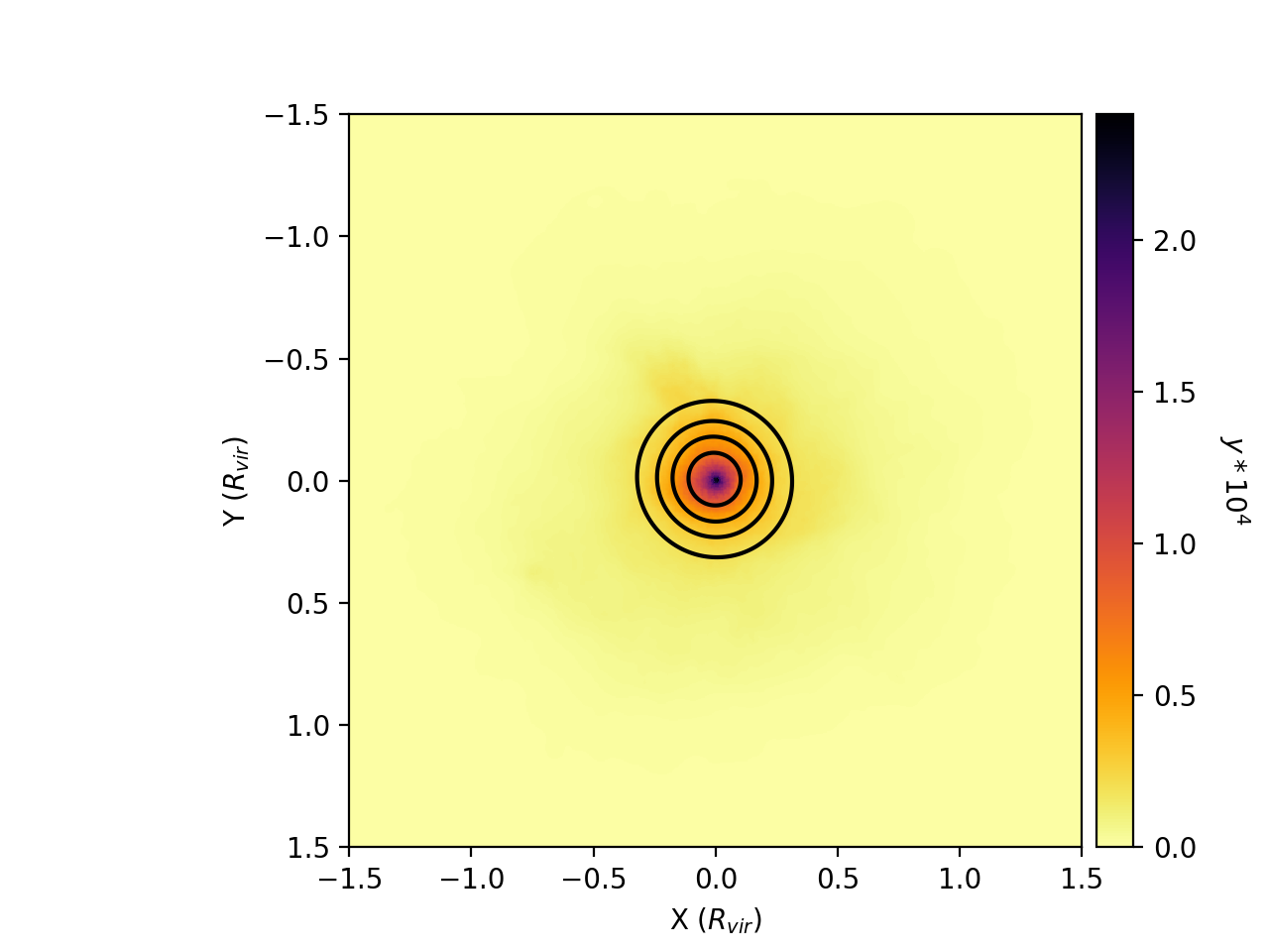
(a)

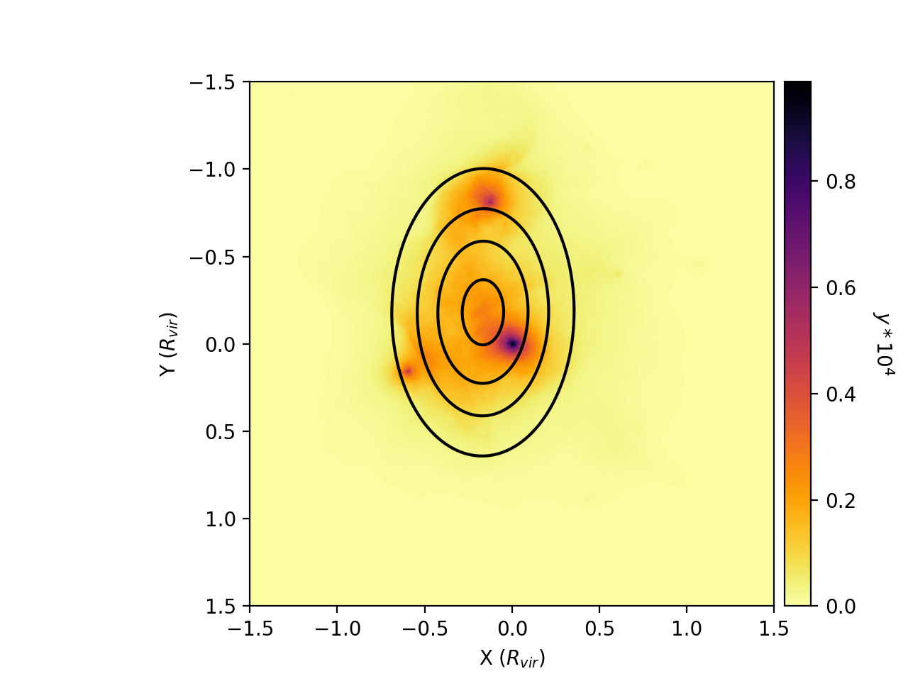
(b)

Figure 2: Best Gaussian fit contour lines (at 20, 40, 60 and 80 per cent of the maximum $y$ value), resulting from the computation of the G parameter. Contours are superimposed to the SZ maps of the example relaxed (#7, left panel) and disturbed cluster (#27, right panel) at redshift $z=0.54$ from the CSF sub-set. The corresponding values of the $G$ parameter are 0.97 and 0.63 for the two clusters, respectively.

To illustrate how the new strip and Gaussian parameters work, we show their different behaviours for an example of relaxed and disturbed cluster (#7 and #27, respectively) from the radiative sub-set at $z=0.54$. Fig. 1 shows the strips defined as above. As expected, the four profiles for the relaxed cluster are similar at all radii ($S=0.09$). On the contrary multiple off-centre peaks characterise the profiles of the disturbed cluster in correspondence of of sub-structures ($S=0.4$). Fig. 2 illustrates the maps of the two clusters and the contour lines representing the Gaussian fit to the maps. The difference between the relaxed and the unrelaxed cluster can be seen from the shapes of the contour lines, which are nearly circular in the first case ($G=0.97$) and elliptical in the second case ($G=0.63$).

Combined parameter, $M$

Finally, we introduce a combined parameter called $M$ (see also Meneghetti et al., 2014; Rasia et al., 2013), where each of the previously defined parameters, denoted generically as $V_{i}$, contributes to $M$ according to a weight, $W_{i}$, related to the efficiency of $V_{i}$ itself in discriminating the dynamical state, as will be detailed later in section 4.2. The analytical definition of the combined parameter is thus:

$$M=\frac{1}{\sum_{i}W_{i}}\left(\sum_{i}W_{i}\frac{\log_{10}(V_{i}^{\alpha_{i}})-<\log_{10}(V_{i}^{\alpha_{i}})>}{\sigma_{\log_{10}(V_{i}^{\alpha_{i}})}}\right)$$ (16)

where the sums extend over all the parameters, and $\alpha_{i}$ is equal to +1 when disturbed clusters are associated to large values of $V_{i}$ (e.g. as in the case of $A$), otherwise it is equal to -1 (e.g. as in the case of $c$). The brackets, $<>$, indicate the average computed over all the clusters, and $\sigma$ is the standard deviation. By definition, we expect negative values for the relaxed clusters, and positive values for the disturbed ones.

4 Results

In this section we first discuss the efficiency of the parameters described in section 3.2, then we analyse their stability by varying the observer line of sight, and thus considering multiple projections of the same cluster, and by changing the angular resolutions of the maps.

4.1 Application of the single parameters

We quantify the efficiency of the morphological parameters with a Kolmogorov-Smirnov test (KS test hereafter) on the distributions of the two populations of relaxed and disturbed objects, as identified from the 3D indicators of the cluster dynamical state (see section 3.1). From this test, we obtain the probability, $p$, that they belong to the same sample. Low values of this probability indicate an efficient discrimination between the two populations.

For all the parameters, the efficiency depends on the aperture radius $R_{ap}$ and in few cases also on the inner radius, such as for the light concentration ratio, or on the FWHM for the fluctuation parameter. As described in the previous section we consider multiple values for all these quantities, and we finally chose those that correspond to the lower value of the probability $p$, averaged over the four redshifts and two sub-samples. The fluctuation parameter returned contradictory results among the redshifts and physics demonstrating that it is not a stable parameter. For this reason, it will be discarded in the rest of the analysis. The minimum probability values for each parameter are listed in Table 2, where we also present the superimposition percentage, $s_{p}$, of the distributions of the two populations and the most efficient aperture radius. The latter turns to be $R_{ap}=0.75R_{vir}$ for the asymmetry parameter, $R_{ap}=0.25R_{vir}$ for the light concentration ratio, and $R_{ap}=R_{vir}$ for all the others.

In general, we find small values for the KS probability, so we can conclude that the relaxed and disturbed populations do not coincide. This implies a good agreement between the dynamical state expected from the 3D indicators and the one inferred from the parameters. Since the results are similar for the NR and the CSF flavours, we conclude that the gas radiative processes do not have significant impact on the SZ maps on which the parameters are computed (consistently with e.g. Motl et al., 2005). Differences are also negligible, within few per cent, in terms of redshift variation.

The light concentration ratio, for which the best inner radius is $r_{1}=0.05R_{vir}$, is the one showing less overlap between the two classes, especially for the CSF flavour (around or less 50 per cent). In our sample, this parameter and the centroid shift are the most efficient as found also in Lovisari et al. (2017). The asymmetry parameter, with a superimposition percentage around 55 per cent is the third most efficient parameter. On the other hand the third-order power ratio, largely used on X-ray maps (see e.g. Rasia et al., 2013), shows a wide overlap between the two populations (around 65 percent, reaching the extreme of 75 per cent). The different response of the power ratio on SZ maps with respect to X-ray maps is mostly caused by its strong dependence on the signal-to-noise ratio (Poole et al., 2006) or gradient of the signal. In SZ, it is particularly affected by the instrumental beam (see e.g. Donahue et al., 2016). Since we have not accounted for all these aspects, that may strong depend on the detection instrument, our conclusions regarding $P_{3}/P_{0}$ should not still be applicable to observational results.

Among the two new parameters we have previously introduced, the strip parameter performs better than the Gaussian fitting parameter. This is also evident by comparing Fig. 3 and 4 where the large overlapping area or the two populations in the $G$ histogram is remarkable. The inefficiency of this parameter is mostly due to the fact that the Gaussian fitting procedure smooths and reduces the impact of small substructures and that $G$ is largely affected by projection effects. Indeed, a dynamically disturbed cluster may appear regular when smoothed and observed from a particular line of sight. This effect leads to the presence of a cospicuous fraction of disturbed clusters identified as relaxed.

Table 2: Results from the application of the $A$, $c$, $\log_{10}(P_{3}/P_{0})$, $w$, $G$ and $S$ parameter to the SZ maps of the sample, for the four analysed redshifts and the two flavours of the simulation. $R_{ap}$ is the best aperture radius as derived from the minimum KS test probability, $p_{m}$. We indicate with $s_{p}$ the superimposition percentage of the distributions of the parameters for the two populations.

		CSF		NR
$R_{ap}\ (R_{vir})$	$z$	$s_{p}$	$p_{m}$	$s_{p}$	$p_{m}$
$A$
$0.75$	0.43	55%	8.7e-13	59%	6.7e-10
	0.54	50%	8.5e-17	49%	1.4e-14
	0.67	58%	1.8e-11	63%	1.2e-09
	0.82	61%	9.2e-12	53%	6.8e-13
$c$
$0.25$	0.43	51%	4.8e-14	57%	2.3e-13
	0.54	47%	2.0e-16	53%	5.9e-13
	0.67	47%	6.8e-17	52%	3.8e-16
	0.82	48%	4.2e-16	57%	3.0e-12
$\log_{10}(P_{3}/P_{0})$
$1.00$	0.43	65%	3.8e-06	69%	1.4e-05
	0.54	75%	8.5e-03	72%	4.0e-03
	0.67	62%	3.5e-09	65%	2.7e-08
	0.82	64%	4.8e-09	67%	2.6e-06
$w$
$1.00$	0.43	53%	5.0e-11	53%	2.0e-11
	0.54	57%	3.5e-11	46%	5.9e-18
	0.67	54%	1.0e-11	59%	7.0e-11
	0.82	55%	9.7e-13	55%	1.5e-10
$S$
$1.00$	0.43	47%	1.3e-16	52%	1.4e-12
	0.54	57%	1.5e-11	66%	4.3e-09
	0.67	66%	3.1e-08	63%	2.7e-08
	0.82	60%	1.5e-10	62%	4.2e-10
$G$
1.00	0.43	70%	1.4e-04	73%	3.5e-03
	0.54	60%	5.7e-10	71%	7.4e-05
	0.67	58%	2.6e-09	72%	5.9e-04
	0.82	68%	1.3e-05	67%	3.9e-05

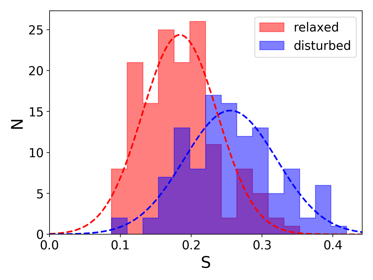
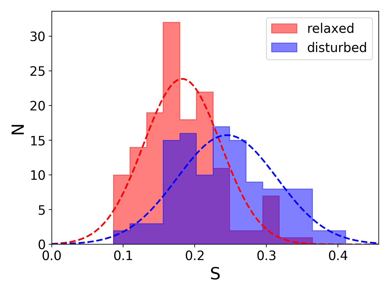
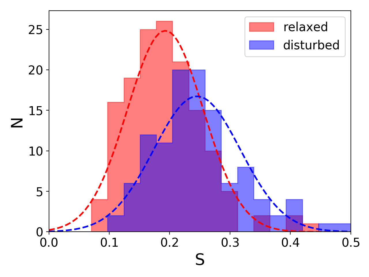
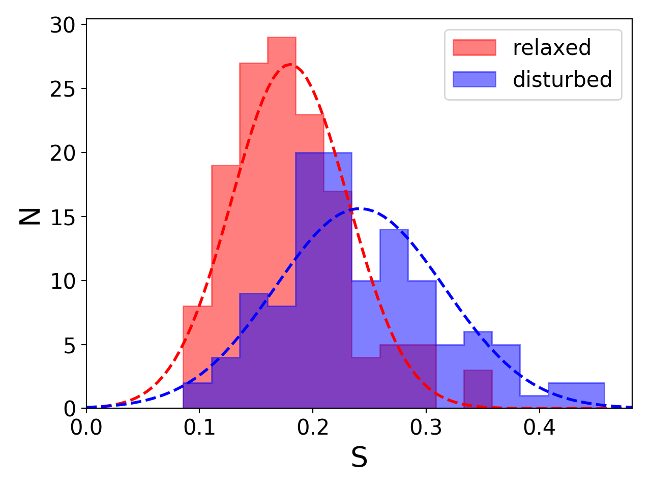
Figure 3: Distribution of $S$ computed inside $R_{ap}=R_{vir}$ at the four different redshifts (0.43 top left, 0.54 top right, 0.67 bottom left and 0.82 bottom right) and for the CSF flavour. The red and blue bars indicate the relaxed and unrelaxed populations respectively, from the a priori discrimination through the 3D indicators. The dashed lines refers respectively to the relaxed (red) and disturbed (blue) populations gaussian fit.

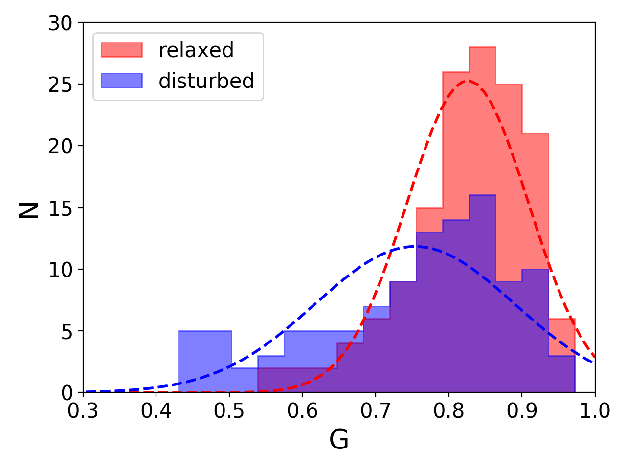
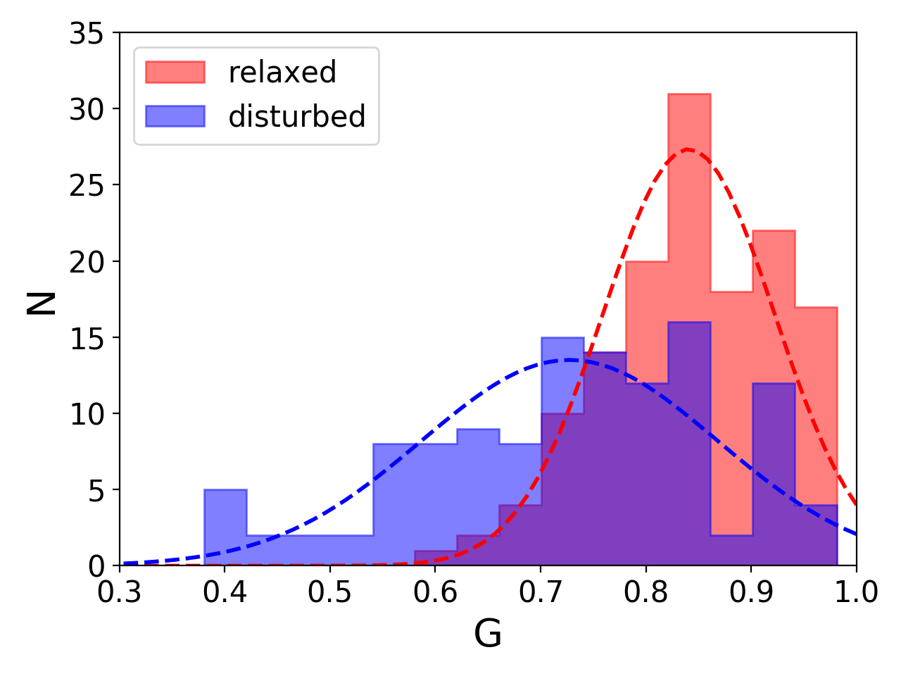
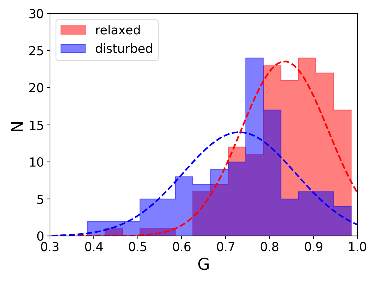
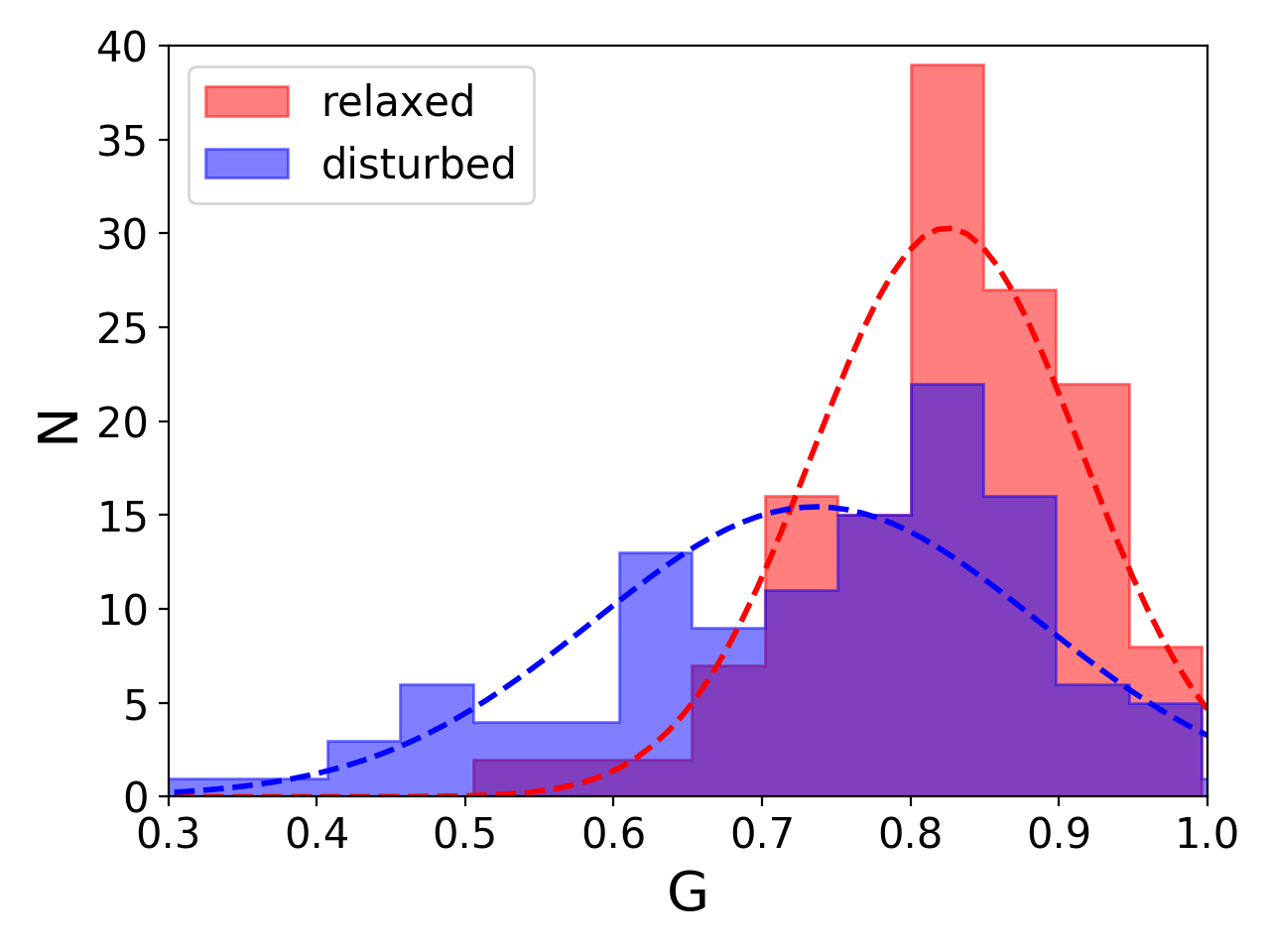
Figure 4: Distribution of the $G$ parameter computed inside $R_{ap}=R_{vir}$ for the CSF flavour (redshift 0.43 top left, 0.54 top right, 0.67 bottom left and 0.82 bottom right). Red and blue bars indicate the relaxed and disturbed populations while red and blue dashed lines refers respectively to the gaussian fit on relaxed and disturbed populations.

4.1.1 Comparison with X-ray results

We compare our morphological parameters, $c$, $w$ and $\log(P_{3}/P_{0})$, with those measured in the mock X-ray Chandra-like maps described in section 2.1. To implement a fair comparison, we re-compute the SZ morphological parameter on the same sub-sample of the MUSIC clusters used for the X-ray analysis. The sample include clusters from the radiative data set at redshifts $z=0.43$ and $z=0.67$ observed from three different lines of sight. We also set the same aperture radii equal to 500 kpc. Finally, for the light concentration ratio $c$ we use an inner radius of 100 kpc.

Table 3 reports the Pearson correlation coefficients between the X-ray and the SZ results, computed for the three parameters on three samples: one considering all the clusters, and two sub-sets built respectively on the relaxed and disturbed populations. The correlation is high only for the light concentration ratio, whose corresponding scatter plot is shown in Fig. 5. In addition to the correlation, one can notice the significant difference in the dynamic range of the X-ray and SZ parameters cause by the different dependence of the two signals on the electron density which is more peaked in X-ray. As expected, the two power ratios poorly correlate given the opposite performances of this parameter in the two bands. No significant correlation is present also in the case of the centroid shift, probably because of the SZ and X-ray dependence on the peaked density of possible sub-structures. A similar comparison was performed in Donahue et al. (2016), based on the application of the parameters on maps of the CLASH sample (see section 1 and Postman et al., 2012), but applying in the SZ maps the same centre position and outer radii used for the X-ray analysis. Also in this work the concentration parameters show a good correlation despite their different dynamic ranges.

Table 3: Pearson correlation coefficients (CC) between the X-ray and SZ results for the three compared parameters $c$, $w$ and $\log(P_{3}/P_{0})$ at redshifts 0.43 and 0.67.

$z=0.43$
parameter	all	relaxed	disturbed
$c$	0.45	0.73	0.18
$\log_{10}(P_{3}/P_{0})$	0.14	0.38	0.12
$w$	0.02	0.23	-0.31
$z=0.67$
parameter	all	relaxed	disturbed
$c$	0.61	0.73	0.41
$\log_{10}(P_{3}/P_{0})$	0.25	0.29	0.09
$w$	0.05	0.46	-0.30

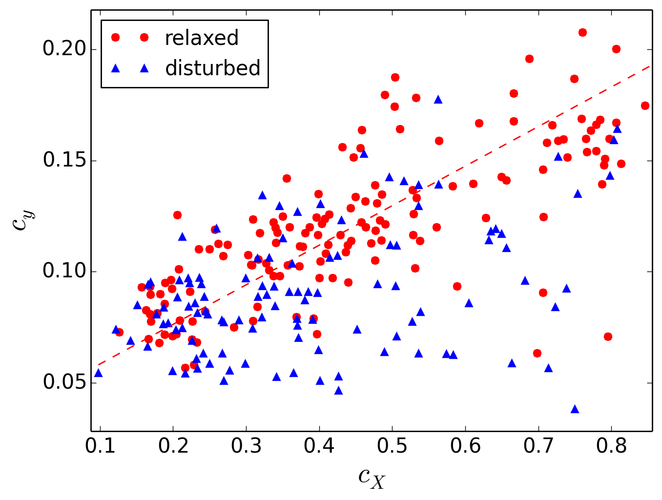
Figure 5: Scatter plot of $c$ parameter computed on X-ray ($c_{X}$) and SZ maps ($c_{y}$) for the NR clusters at $z=0.67$. Relaxed clusters are marked as red circles, disturbed ones are marked as blue triangles. The red dashed line shows the best robust fit for the relaxed clusters only.

4.2 Application of the combined parameter

We compute the combined morphological parameter $M$, introduced in section 3, following equation 16, where in particular, each $V_{i}$ parameter is measured within its most efficient aperture radius (Table 2), and its weight $W_{i}$ is the absolute value of the logarithm of the corresponding KS probability, $p_{i}$, averaged over the four redshifts and two cluster sub-sets (Table 4):

$$W_{i}=|\log_{10}(p_{i})|\ .$$ (17)

With this choice the parameters showing a higher efficiency (i.e. with low values of $p_{i}$) contribute the most to $M$. The heaviest parameters are the light concentration ratio and the centroid shift. On the contrary, $P_{3}/P_{0}$ has the least influence. This suggests that this parameter could be neglected in real applications on observed SZ maps, without affecting significantly the final value of $M$.

Table 4: Average over the redshifts and flavours of the weights for the single parameters used in the definition of the $M$ parameter.

parameter	$W_{i}$
$A$	9.63
$c$	12.31
$\log_{10}(P_{3}/P_{0})$	2.80
$w$	10.38
$S$	8.10
$G$	3.31

The distributions of $M$ for the relaxed and unrelaxed clusters are shown in Fig. 6; the corresponding overlap percentages and probabilities from the KS test are listed in Table 5. It is noticeable the efficiency improvement of this parameter over each single parameter: the contamination level is of the order of 22 per cent for the relaxed population and 28 per cent for the disturbed population.

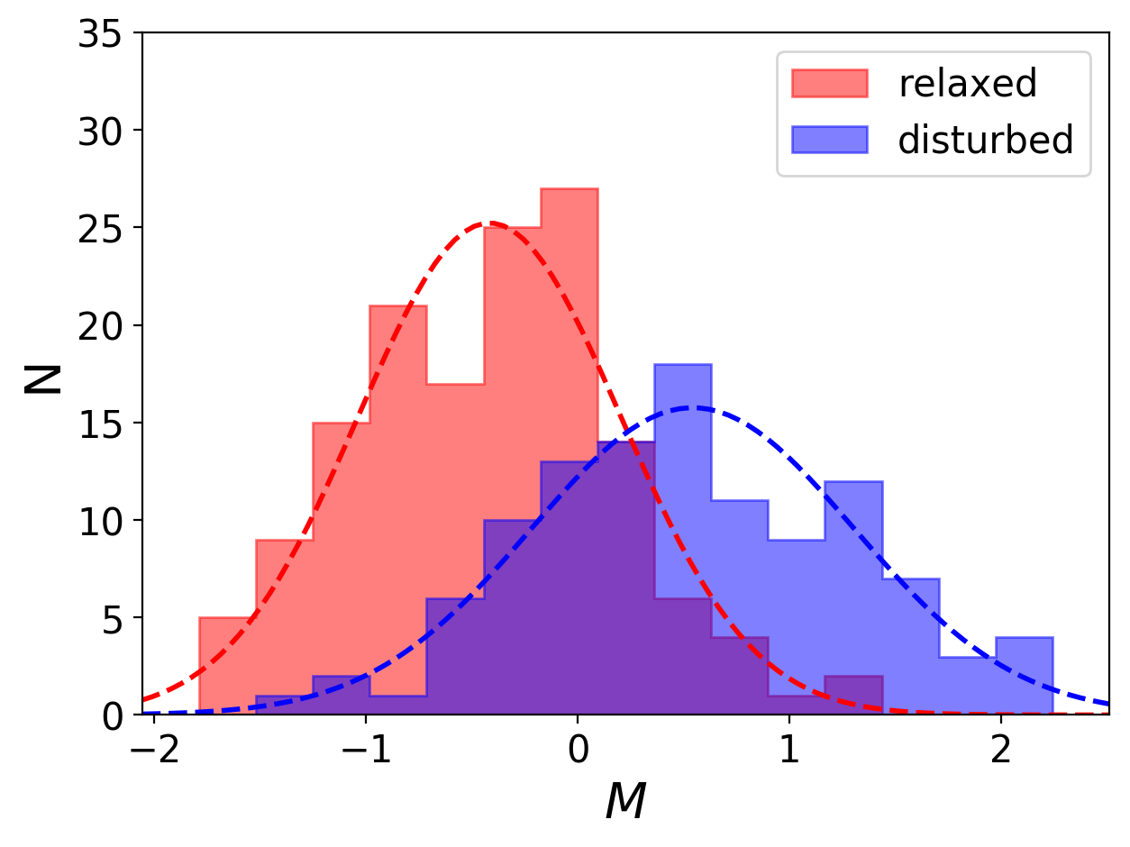
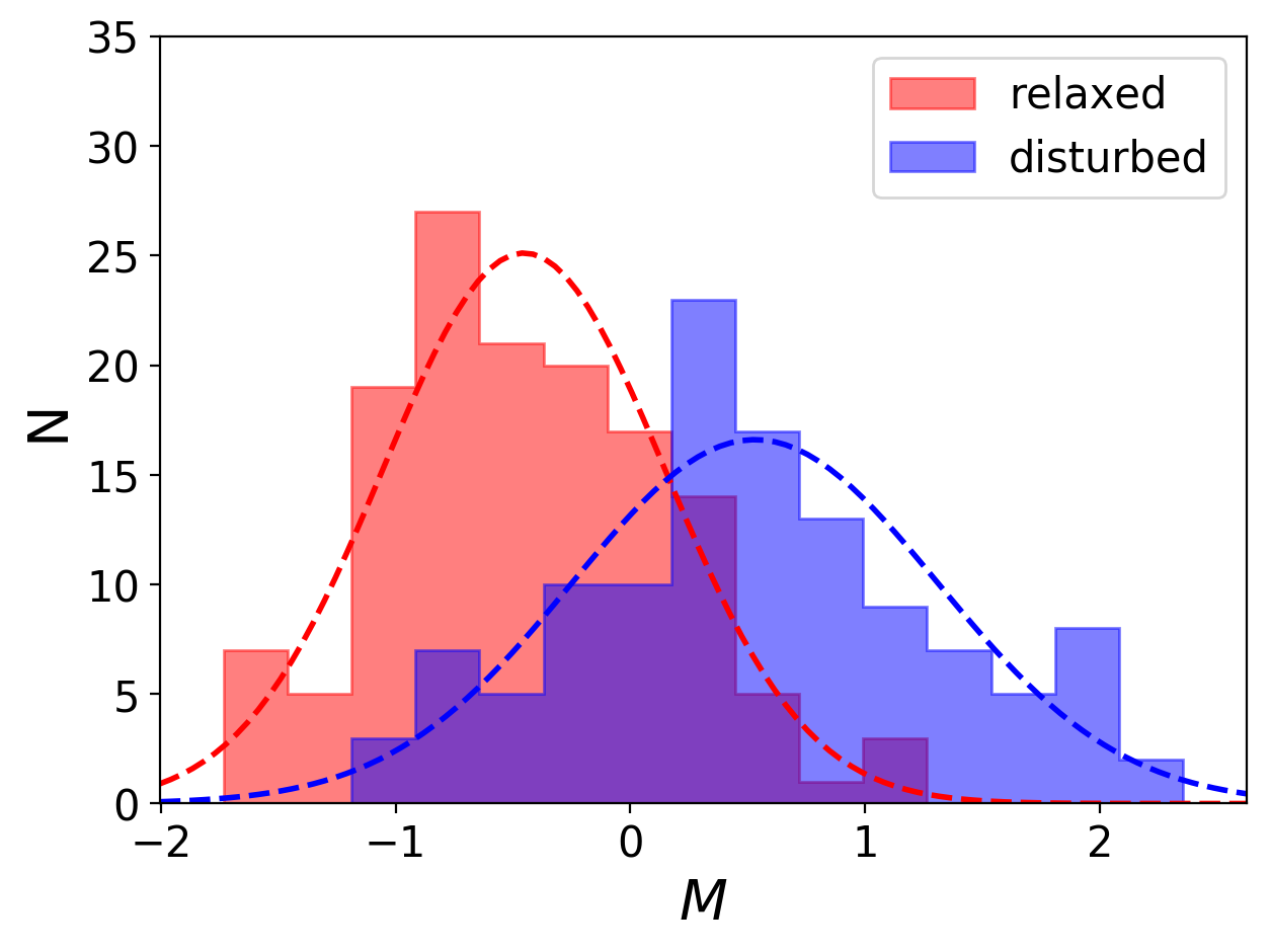
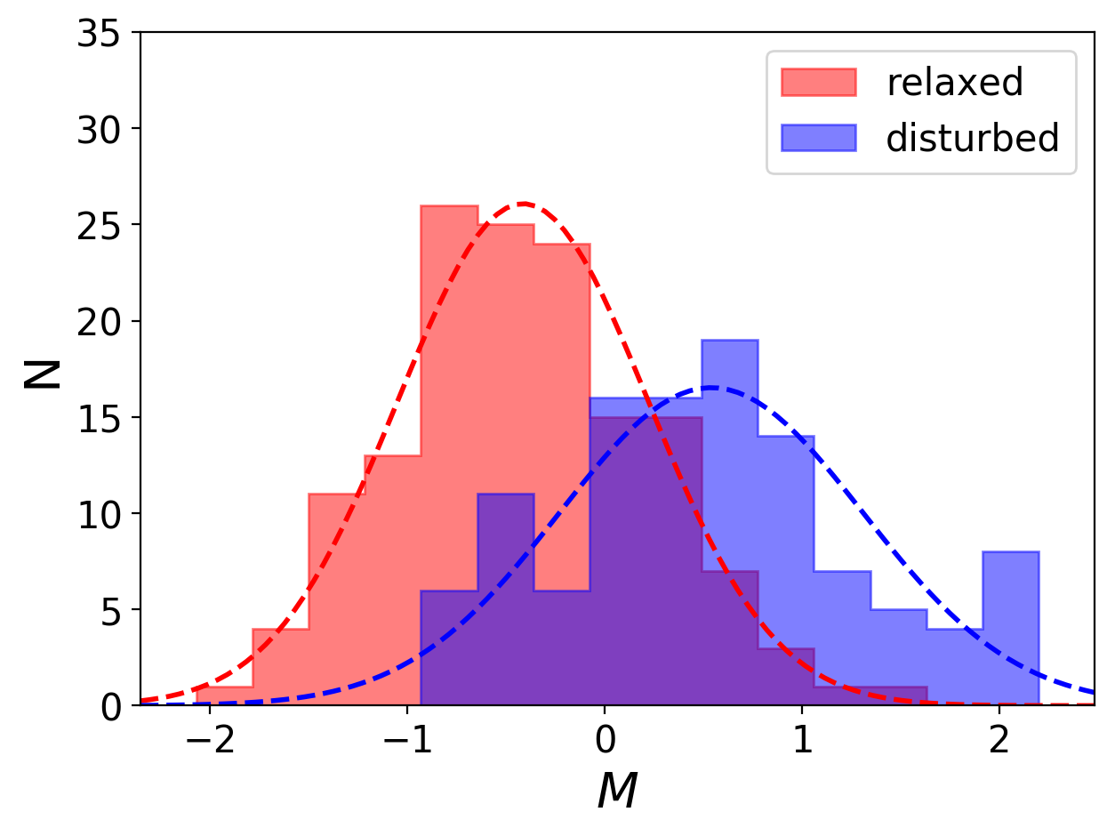
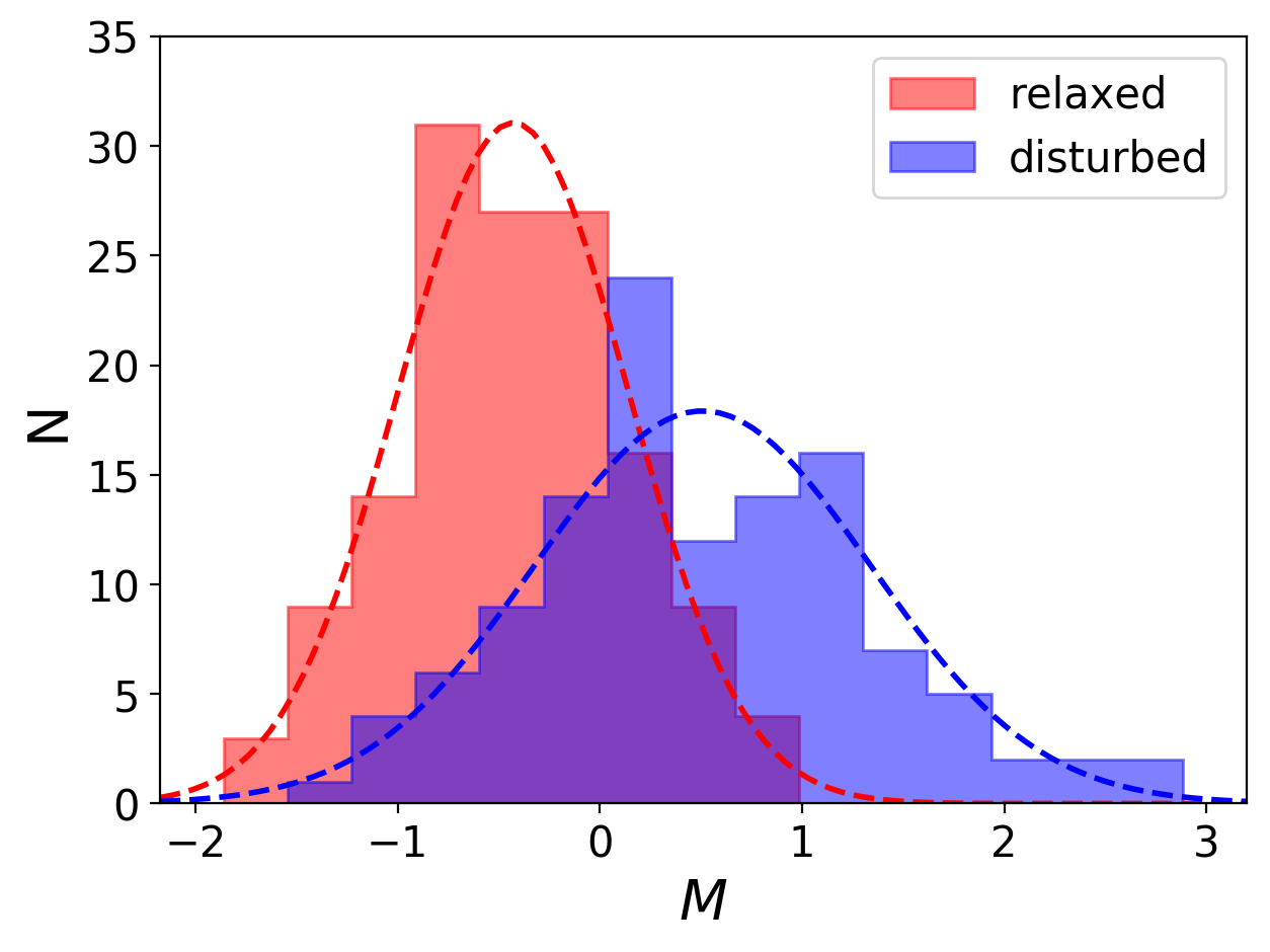
Figure 6: Distributions of $M$ computed with K-S suggested aperture radii at the four different redshifts (0.43 top left, 0.54 top right, 0.67 bottom left and 0.82 bottom right) for the CSF flavour. The red and blue bars indicate the relaxed and unrelaxed populations respectively, determined from the 3D indicators.

Table 5: Superimposition percentage $s_{p}$ between the distributions of relaxed and disturbed clusters, and associated KS probability $p_{m}$ for the $M$ parameter.

$z$	CSF		NR
	$s_{p}$	$p_{m}$	$s_{p}$	$p_{m}$
0.43	47%	4.2e-18	50%	3.0e-14
0.54	45%	7.7e-19	48%	2.5e-16
0.67	51%	1.3e-16	51%	1.2e-13
0.82	49%	3.8e-16	51%	1.0e-14

4.3 Test on the stability of the parameters

To check the stability of all parameters, we produce SZ maps of two relaxed and two disturbed clusters from our CSF sub-set at $z=0.54$ and $z=0.82$ along 120 lines of sight. We checked that the results are similar for the NR sub-set and at the remaining redshifts. Specifically, we consider lines of sight spaced in uniform steps of 9^∘. The six morphological parameters and the combined one are applied to all these maps and their distributions are drawn. The corresponding standard deviations are an estimate of the stability of the parameter. We list the results in Table 6. For all parameters, disturbed clusters tend to have a higher dispersion with respect to the relaxed ones, as expected because of projection effects. The mean value of the standard deviation of $M$, with respect to the four clusters at both redshifts, is $<{\sigma_{M}}>=0.41$. We consider this value as the uncertainty of the $M$ parameter. For this reason all clusters with $M$ between -0.41 and 0.41 might be a mixture of relaxed and disturbed objects.

Table 6: Standard deviations of all morphological parameters for two relaxed (#17 and #267) and two disturbed (#44 and #277) clusters at redshift 0.54 and 0.82, as derived from the SZ maps computed at 120 different lines of sight.

parameter	$z=0.54$				$z=0.82$
	relaxed		disturbed		relaxed		disturbed
	#17	#267	#44	#277	#17	#267	#44	#277
$A$	0.030	0.040	0.060	0.050	0.060	0.040	0.100	0.080
$c$	0.007	0.002	0.008	0.013	0.014	0.005	0.008	0.015
$\log_{10}(P_{3}/P_{0})$	0.620	0.430	0.600	0.430	0.470	0.630	0.400	0.510
$w$	0.002	0.0007	0.004	0.003	0.001	0.001	0.005	0.008
$S$	0.030	0.020	0.060	0.020	0.040	0.020	0.070	0.040
$G$	0.070	0.060	0.050	0.070	0.040	0.070	0.070	0.130
$M$	0.28	0.30	0.43	0.37	0.49	0.26	0.57	0.58

4.4 Effects of the angular resolution

Current SZ experiments cannot reproduce the angular resolution of our maps (see section 1). In this section we want to verify the impact of the resolution on the performance of the morphological parameters. We thus reduce the SZ signal of our maps by applying a Gaussian smoothing. We choose three FWHMs similar to the typical resolution achieved by existing telescopes in the millimetric band: 20 arcsec for IRAM 30-m telescope, 1 arcmin for SPT 10-m telescope and 5 arcmin for the Planck telescope. We perform the convolution only on CSF maps at $z=0.54$ and $z=0.82$.

The superimposition percentages of the histograms of the relaxed and unrelaxed classes for the $M$ parameter are listed in Table 7. The overlap is expected to increase with the value of the FWHM (i.e. with increasing resolution), nevertheless we find a decrease of 1 per cent and 3 per cent of the superimposition at 20 arcsec and 1 arcmin, respectively. This may be explained by considering that the $M$ parameter depends on the overall morphology, thus small-scale effects are negligible at resolutions of the order of few arcminutes. With respect to the individual parameters, we found that the angular resolution barely affects their ability to distinguish between the two dynamical classes when the morphological parameters are sensitive to the properties of the cluster core, such as the light concentration ratio. At the same time, the resolution has a large impact on the results derived from the parameters built to enhance the presence of substructures such as the strip parameter.

Table 7: Superimposition percentages of $M$ with respect to the FWHM of the Gaussian filter applied to the maps to simulate a decreasing angular resolution.

FWHM (arcsec)	$z$
	0.54	0.82
$20$	43%	48%
$60$	41%	46%
$300$	51%	54%

5 Morphology and hydrostatic mass bias

We investigate, here, the correlation between the morphological parameter $M$ and the deviation from the hydrostatic equilibrium in the ICM. For each simulated cluster, we define the hydrostatic mass bias as follows:

$$b_{M}=(M_{500,HSE}-M_{500})/M_{500}.$$ (18)

In the expression above, $M_{500}$ is the mass obtained by summing the gas and DM particles inside $R_{500}$. $M_{500,HSE}$ is the mass computed under the assumption of the hydrostatic equilibrium expressed as:

$$M_{500,HSE}=-\frac{k_{B}Tr}{G\mu m_{H}}\left(\frac{d\text{ln}\rho}{d\text{ln}r}+\frac{d\text{ln}T}{d\text{ln}r}\right)\ ,$$ (19)

where $k_{B}$ and $G$ are the Boltzmann and gravitational constants, $r$ is the radius from the centre of the cluster, $\mu$ is the mean molecular weight, $m_{H}$ the hydrogen mass, $\rho$ the density and $T$ the mass-weighted temperature (Sembolini et al., 2013). The mass bias has already been analysed in many works on hydrodynamical simulations, lensing and X-ray observations like Kay et al. (2004), Rasia et al. (2006), Nagai et al. (2007), Jeltema et al. (2008), Piffaretti & Valdarnini (2008), Zhang et al. (2010), Meneghetti et al. (2010), Becker & Kravtsov (2011) and Sembolini et al. (2013).

The sources of the asymmetry in the ICM distribution should also impact the hydrostatic equilibrium. We, therefore, investigate correlation between the absolute value of the mass bias $|b_{M}|$ and the $M$ parameter in our sample. The results are reported in Fig. 7 for CSF clusters (NR clusters have a similar behaviour). For each redshift and simulated sub-set (NR/CSF) we compute the Pearson correlation coefficient and report the results in Table 8. This coefficient is almost always below 0.30. This rather weak correlation leads us to conclude that there is no strong connection between $|b_{M}|$ and the morphology of the cluster as quantified by our indicators.

This result suggest that the amplitude of the mass bias is not tightly connected to the dynamical state of a cluster. However, It is worth to stress that the mass bias values we have used for this comparison are computed within $R_{500}$. This may be a limiting factor, since a different radial value could be used. For this reason we compute the median profiles of the mass bias along the cluster radius, for the relaxed and disturbed clusters segregated according to the 3D parameters. We show these profiles in Fig. 8, where a consistent superimposition between the two populations within the median absolute deviation can be seen from 0.8 $R_{500}$ and beyond. It can be also seen that the scatter of the median profile for the disturbed clusters is higher, since they are expected to show a more significant deviation from the hydrostatic equilibrium with respect to the relaxed ones. Among the others, Biffi et al. (2016) already investigated the median radial profile of the mass bias, using a small sample of 6 relaxed and 8 disturbed clusters from a simulation which also includes feedback from AGN. They find that the radial median profiles of the relaxed and disturbed clusters have very little differences, as in our case, and that the mass bias is slightly lower (in absolute value) for the relaxed clusters.

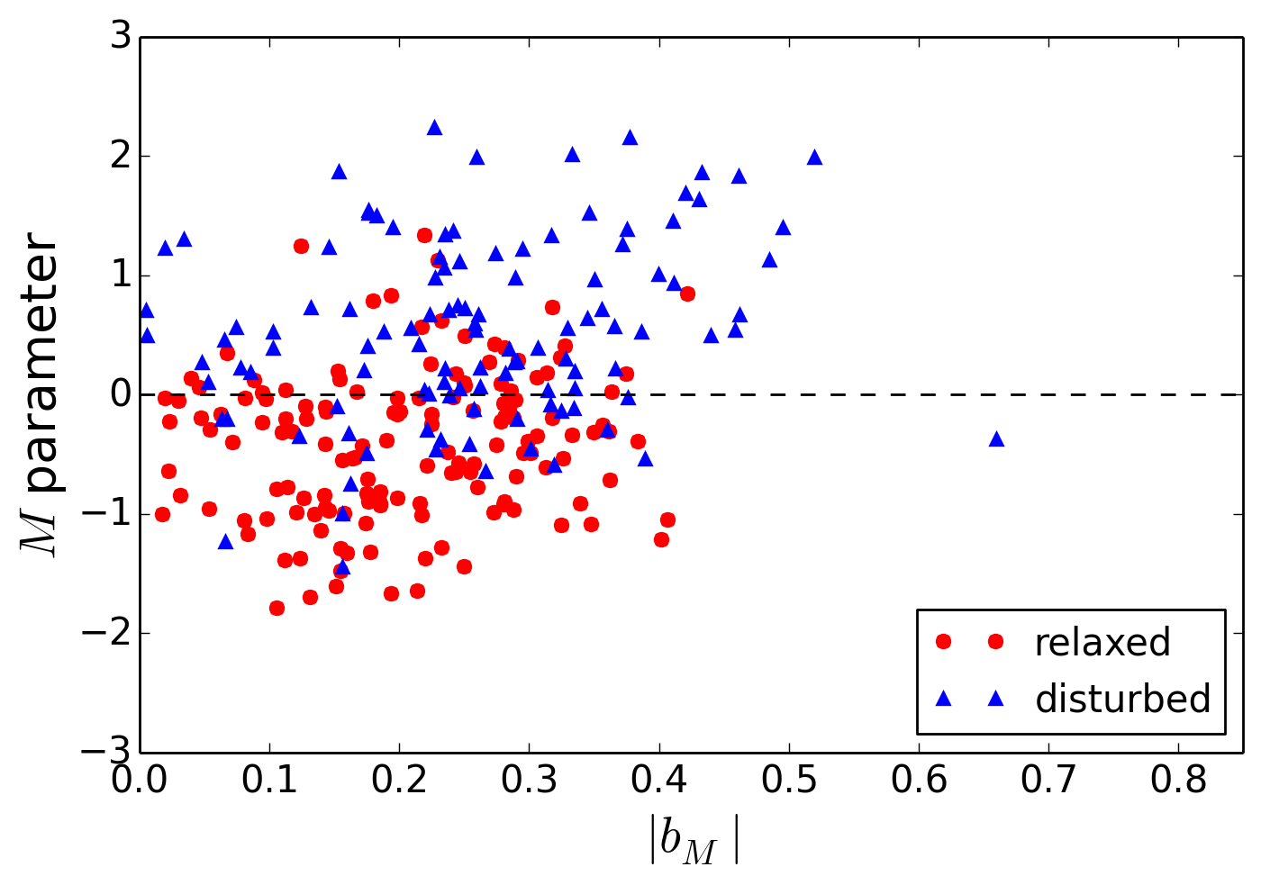
(a)

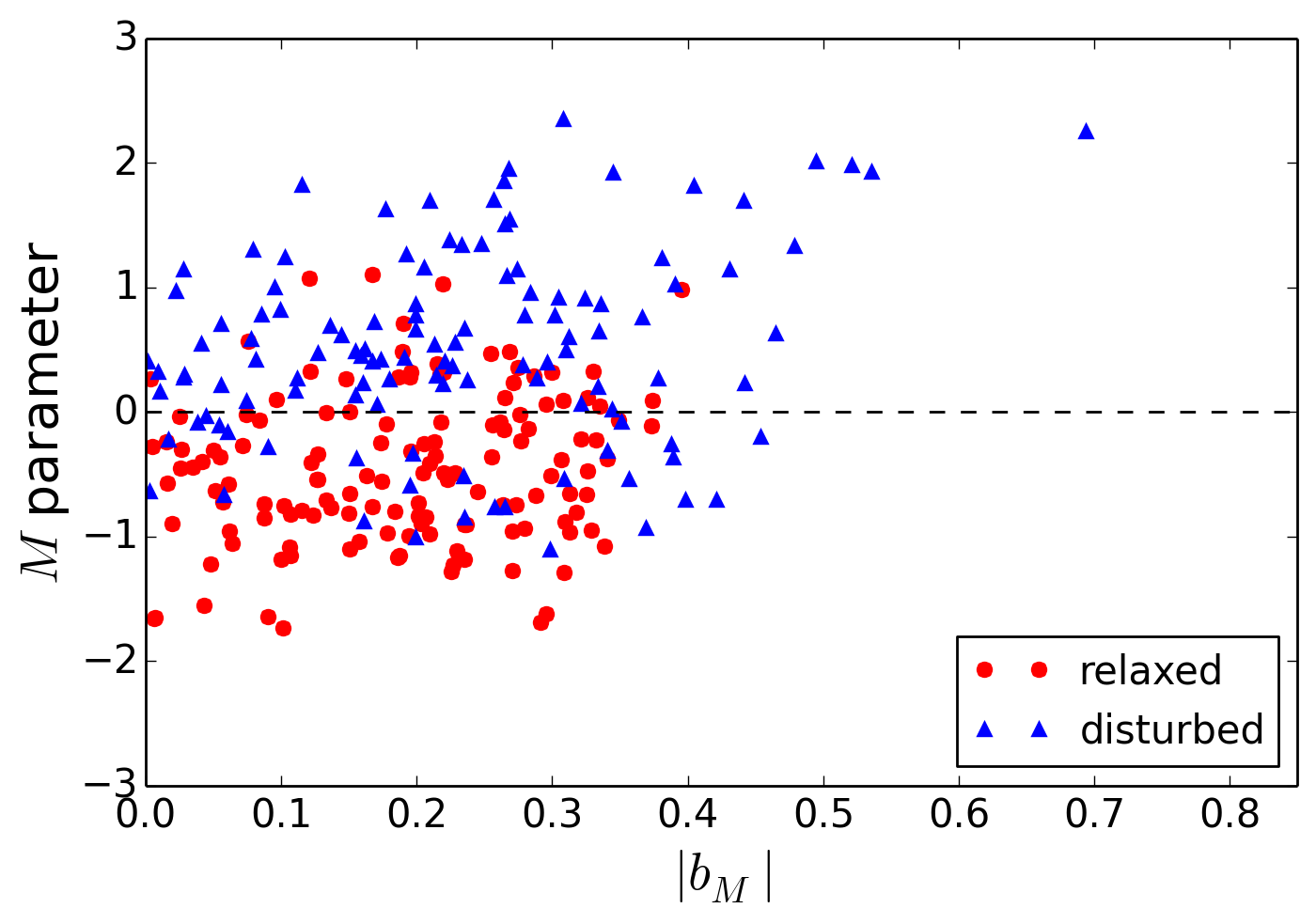
(b)

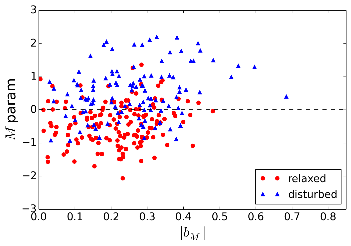
(c)

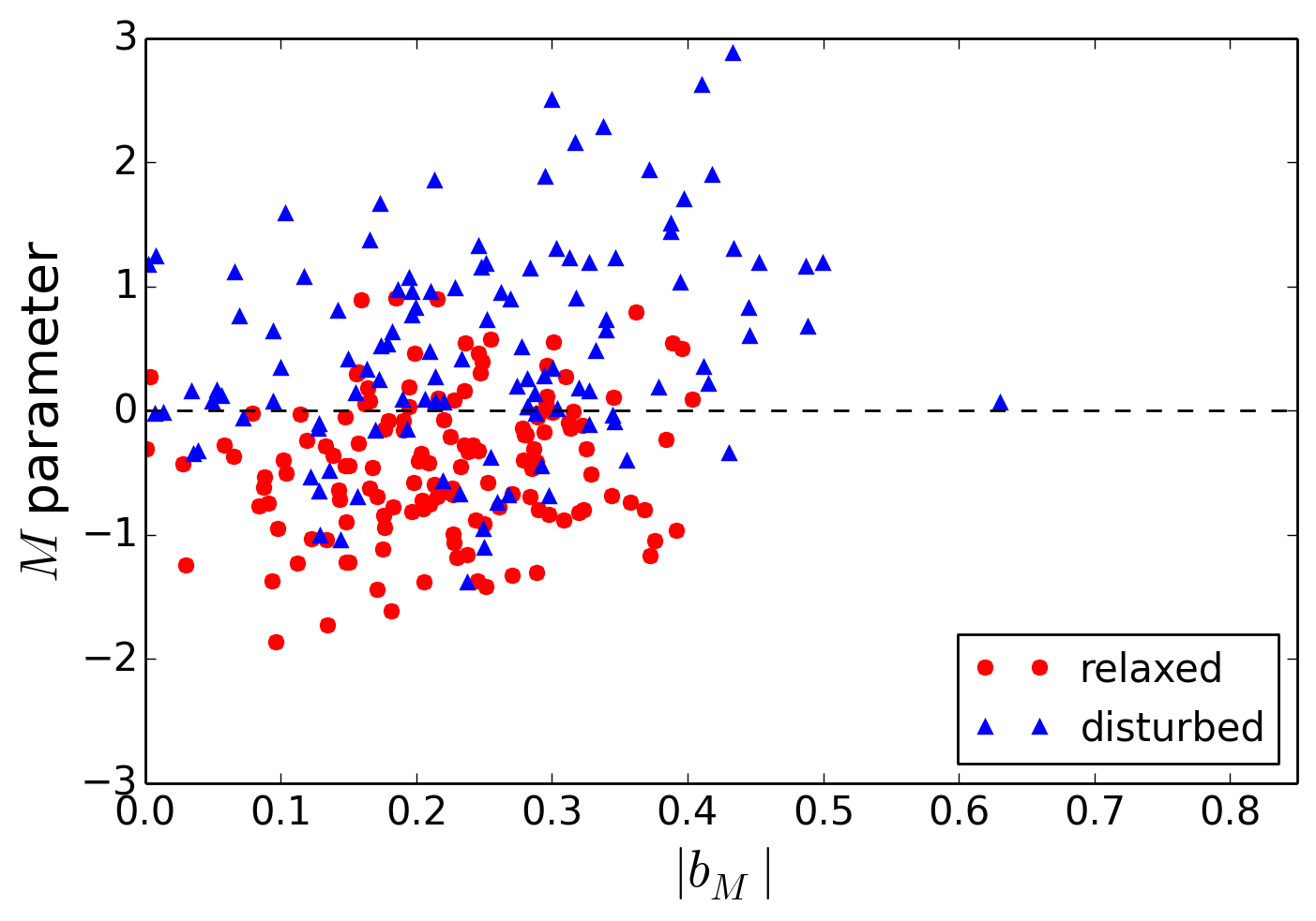
(d)

Figure 7: Mass bias absolute value $|b_{M}|$ plotted against the $M$ combined parameter for the CSF flavour at redshifts 0.43, 0.54, 0.67 and 0.82 (shown in panels (a), (b), (c) and (d), respectively). Relaxed/disturbed clusters are marked with red filled circles/blue filled triangles. The black dashed line marks the threshold ($M=0$) for the $M$ parameter.

Table 8: Pearson correlation coefficients (CC) found between $|b_{M}|$ and $M$ for all considered redshifts and flavours.

$z$	CC
	CSF	NR
0.43	0.29	0.28
0.54	0.27	0.29
0.67	0.26	0.30
0.82	0.27	0.37

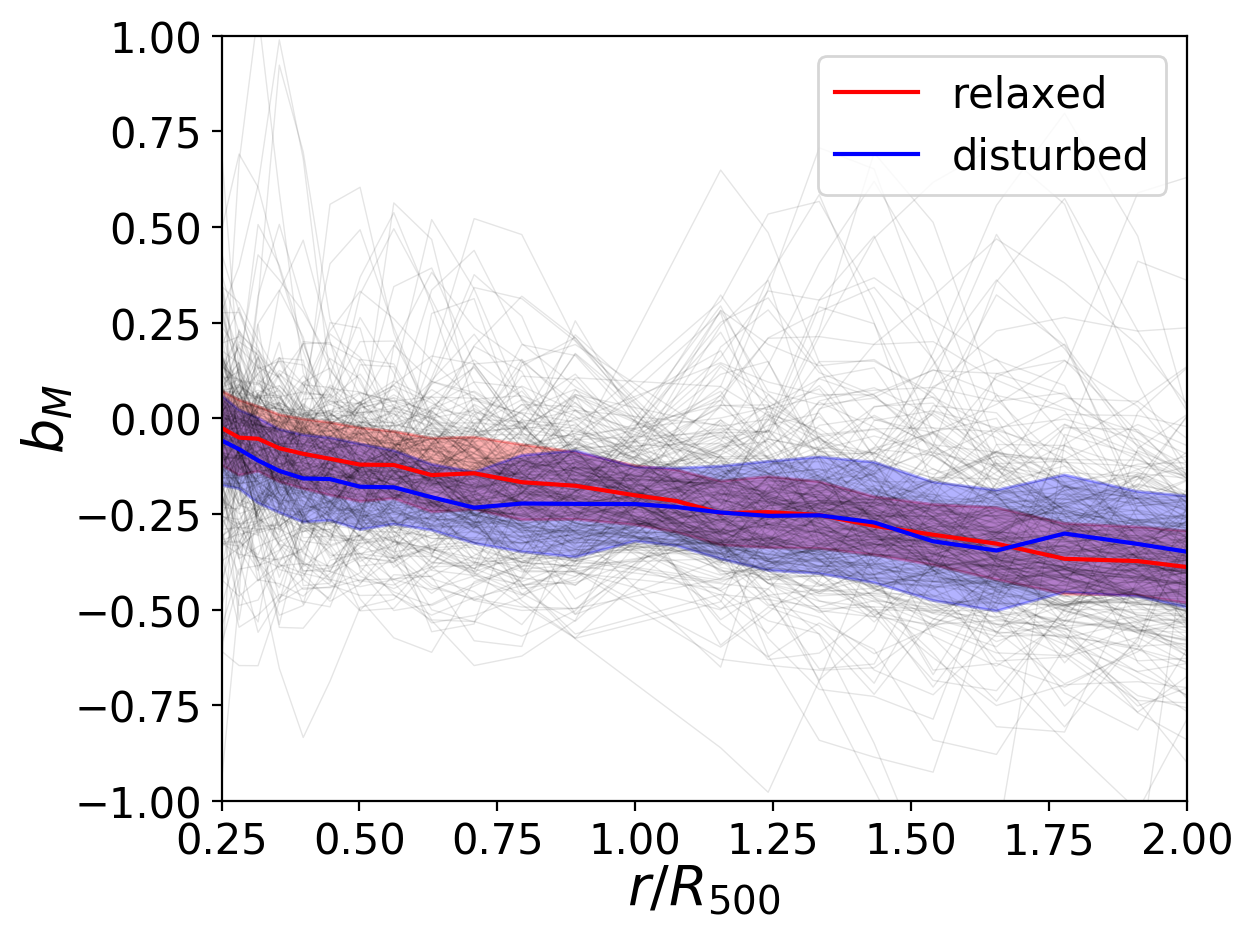
Figure 8: Radial median profiles of $b_{M}$ for relaxed (red) and disturbed (blue) clusters of the sample at redshift $z=0.54$ and CSF flavour. Gray shaded lines represents the highly scattered single cluster profiles from which the median are computed. The coloured regions indicate the median absolute deviations of the median profiles.

6 Morphology and projected SZ-CM offset

An additional indicator of the dynamical state which can be computed from observations, is the offset between the positions of the brightest cluster galaxy (BCG) and the X-ray peak. The goodness of this parameter to infer the dynamical state has been proven through the years by both observations (see e.g. Katayama et al., 2003; Patel et al., 2006; Donahue et al., 2016; Rossetti et al., 2016) and simulations (see e.g. Skibba & Macciò, 2011). An equivalent indicator on SZ maps has been recently investigated by Gupta et al. (2017) using the Magneticum simulation. Indeed, in the aforementioned work they computed the projected offset between the centre of gravitational potential of the cluster and the SZ peak, normalised to $R_{500}$.

We compute the projected offset $D_{y-CM}$ between the centroid of the $y$-map inside $R_{vir}$ and the centre of mass of the cluster (that at first approximation coincides with the BCG), normalised to $R_{vir}$. The correlation between $D_{y-CM}$ and our combined morphological parameter is then analysed, in order to compare pure morphological information with an observational dynamical state-driven quantity. The correlation is of the order of 80%, as shown in Table 9. In Fig. 9 the correlation for the CSF sub-set is shown; no significant deviations are found in the NR sample. The strong correlation between $M$ and $D_{y-CM}$ suggests that morphology is closely related to the dynamical state. Therefore, under the assumption of coincidence between CM and BCG positions, this parameter can be easily inferred from joint optical and SZ observations. Being the threshold value for the $M$ parameter known, we derive the corresponding average threshold value for $D_{y-CM}$ of 0.070 by interpolating on the best-fit curve. This allows us to infer that the cluster is relaxed(unrelaxed) if $D_{y-CM}$ is below(above) this value. Moreover this threshold value is consistent with the one found by Meneghetti et al. (2014) referring to the 3D offset between the position of the CM and the minimum of the gravitational potential. Following the same approach used for the analysis of the $M$ parameter contaminants, we find that there is an average of 25%(20%) contaminant clusters in the relaxed(disturbed) population. Being this contamination lower than the corresponding one for the $M$ parameter, we conclude that this 2D offset performs better in discriminating the dynamical state of the clusters. Considering the averaged deviation of $M$, $<{\sigma_{M}}>=0.41$ we derive through an interpolation the corresponding deviation of $D_{y-CM}$ of $<{\sigma_{D}}>=0.029$. Hence, as a final criterion, we consider a cluster as relaxed if $D_{y-CM}<0.041$ and disturbed if $D_{y-CM}>0.099$.

Table 9: Pearson correlation coefficients (CC) between $D_{y-CM}$ and the $M$ combined parameter for all the analysed redshifts and flavours.

$z$	CC
	CSF	NR
0.43	0.78	0.78
0.54	0.77	0.75
0.67	0.76	0.79
0.82	0.75	0.75

(a)

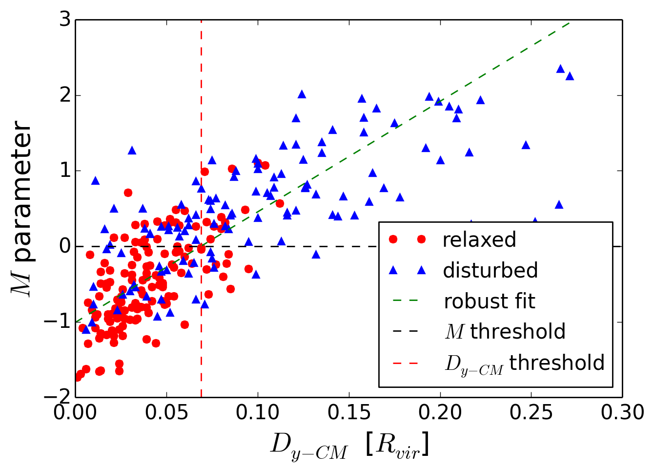
(b)

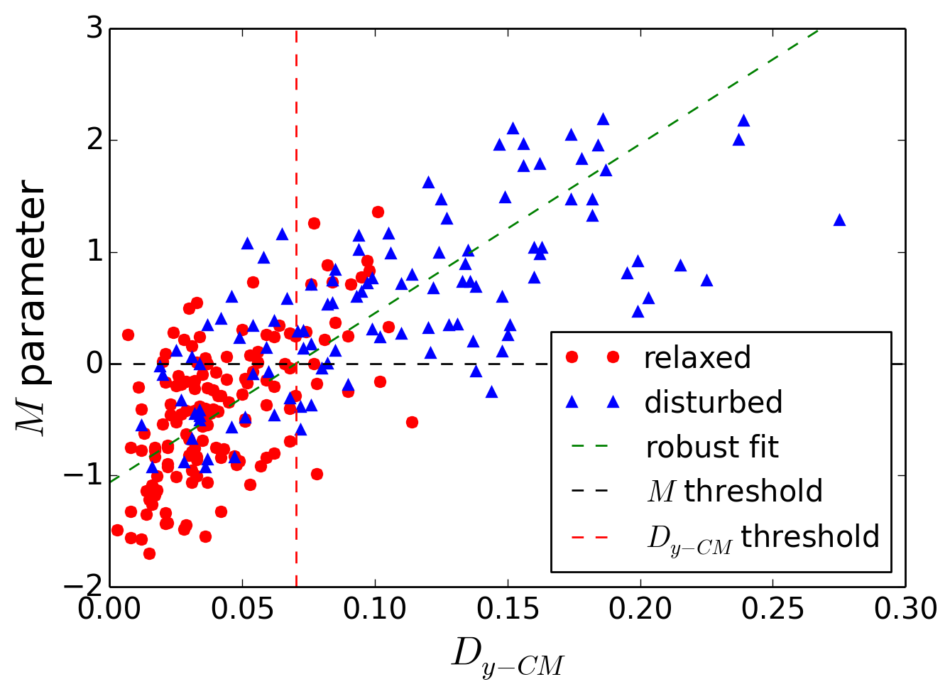
(c)

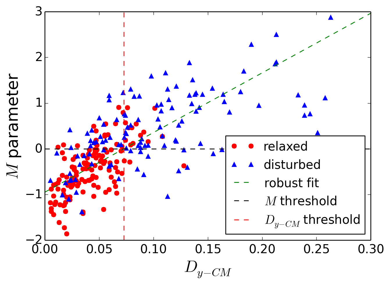
(d)

Figure 9: Scatter plots of the $D_{y-CM}$ 2D offset vs the combined parameter $M$. Panels (a), (b), (c) and (d) refer to redshifts 0.43, 0.54, 0.67 and 0.82, respectively. Black horizontal and red vertical dashed lines mark the $M$ and $D_{y-CM}$ parameters thresholds, respectively. Green dashed lines show the best robust fit for all the clusters.

7 Conclusions

The study of cluster morphology through several indicators allows to analyse large amounts of data from surveys in different spectral bands and will be crucial for the understanding of the structure formation scenario. This topic has been already studied in the X-ray band, and we approach it here for the first time using SZ maps, opening a new window on cluster morphology in the microwave band. To this purpose, we analyse the application of some morphological parameters on the synthetic SZ maps of $\sim 260$ massive clusters extracted from the MUSIC-2 data set, taking non-radiative and radiative physical processes into account, and studying four different redshifts. The clusters have been a priori classified as relaxed and disturbed using two standard 3D theoretical indicators: $\Delta_{r}$ and $M_{sub}/M_{vir}$ related respectively to the offset between the peak of the density distribution and the centre of mass, and to the mass ratio between the biggest sub-structure and the total halo. We use a set of observational parameters derived from X-ray literature and two new ones (the Gaussian fit and the strip parameters), testing their performances when applied on the SZ maps in terms of efficiency and stability. All the parameters have been properly combined into a single morphological estimator $M$. The discriminating power of M, is found to be higher respect to the single parameters. Moreover we studied its possible correlations with the hydrostatic mass bias and with the projected offset between the position of the SZ peak and the position of the centre of mass of the cluster.

The results we achieved can be summarized as follows:

• Few morphological parameters (namely the light concentration, the centroid shift and the asymmetry) are efficient when applied to SZ maps, as they are for the X-ray maps. This may be because of their sensitivity to the very central core region morphology, which has been already well probed both in SZ and in X-ray imaging. Nevertheless, other parameters have been proven to be less efficient with respect to the application to X-ray map, as e.g. the third-order power ratio and the fluctuation parameter, which, in particular, shows an unexpected behaviour in our case;

• The combined parameter $M$ shows less overlap of the two dynamical state populations with respect to any of the single parameters. Its threshold value $M=0$ properly discriminates between relaxed and disturbed dynamical states. The contaminant percentages are 22 per cent for disturbed clusters, and 28 per cent for relaxed, respectively. We have estimated the error for the parameter as the standard deviation, computed from the estimation of M on maps projected along many different line of sight, finding it to be $\overline{\sigma_{M}}=0.41$;

• By varying the angular resolution of the maps, involving a Gaussian smoothing, the overlap of the two populations determined through the combined parameter shows an expected increase at the lowest resolution we have tested (5 arcmin). Nevertheless, when the resolution is below or equal to 1 arcmin the performances are improved. This may be because of the small fluctuation suppression on the maps due to the convolution with the beam resolution;

• The $M$ parameter, which has been proven to be a good proxy of the dynamical state, shows a weak correlation with the mass bias, in agreement with other analyses found in literature;

• The 2D spatial offset $D_{y-CM}$ between the SZ centroid and centre of mass of the cluster is strongly correlated with its morphology and dynamical state, with a correlation coefficient of $\sim 80$ per cent, This correlation shows no significant dependence on the cluster redshift or on the simulation flavour. We propose this indicator as a fast-to-compute observational estimator of the cluster dynamical state. From the threshold value of 0.070 – inferred by interpolating on the best-fit relation linking $D_{y-CM}$ with $M$ – we get a contamination of 25 and 20 per cent of the relaxed and disturbed samples, respectively. This reduced contamination suggests a slightly better segregating power of this parameter as compared with $M$. As a final criterion to distinguish between the two populations, we conclude that a cluster having $D_{y-CM}<0.041$ can be classified as relaxed, while it can be classified as non-relaxed if $D_{y-CM}>0.099$.

We plan to apply the analysis outlined in this work to more realistic data, namely by processing the current synthetic maps through the NIKA-2 instrument pipeline, in order to take the impacts of astrophysical and instrumental contaminants into account.

References

- Adam et al. (2014) Adam R., et al., 2014, A&A, 569, A66
- Adam et al. (2018) Adam R., Adane A., Ade P. A. R., André P., Andrianasolo A., Aussel H., Beelen A., et al., 2018, A&A, 609, A115
- Andrade-Santos et al. (2017) Andrade-Santos F., et al., 2017, ApJ, 843, 76
- Baldi et al. (2017) Baldi A. S., De Petris M., Sembolini F., Yepes G., Lamagna L., Rasia E., 2017, MNRAS, 465, 2584
- Becker & Kravtsov (2011) Becker M. R., Kravtsov A. V., 2011, ApJ, 740, 25
- Biffi et al. (2014) Biffi V., et al., 2014, MNRAS, 439, 588
- Biffi et al. (2016) Biffi V., et al., 2016, ApJ, 827, 112
- Bleem et al. (2015) Bleem L. E., et al., 2015, ApJS, 216, 27
- Böhringer et al. (2010) Böhringer H., et al., 2010, A&A, 514, A32
- Booth (2000) Booth R. S., 2000, in Schürmann B., ed., ESA Special Publication Vol. 451, Darwin and Astronomy : the Infrared Space Interferometer. p. 107
- Borgani (2008) Borgani S., 2008, in Plionis M., López-Cruz O., Hughes D., eds, Lecture Notes in Physics, Berlin Springer Verlag Vol. 740, A Pan-Chromatic View of Clusters of Galaxies and the Large-Scale Structure. p. 24 (arXiv:astro-ph/0605575), doi:10.1007/978-1-4020-6941-3_9
- Buote & Tsai (1995) Buote D. A., Tsai J. C., 1995, ApJ, 452, 522
- Buote & Tsai (1996) Buote D. A., Tsai J. C., 1996, ApJ, 458, 27
- Calvo et al. (2016) Calvo M., et al., 2016, JLTP, 184, 816
- Carlstrom et al. (2002) Carlstrom J. E., et al., 2002, ARA&A, 40, 643
- Cassano et al. (2010) Cassano R., Ettori S., Giacintucci S., Brunetti G., Markevitch M., Venturi T., Gitti M., 2010, ApJ, 721, L82
- Chang et al. (2009) Chang C. L., et al., 2009, in Young B., Cabrera B., Miller A., eds, American Institute of Physics Conference Series Vol. 1185, American Institute of Physics Conference Series. pp 475–477, doi:10.1063/1.3292381
- Conselice (2003) Conselice C. J., 2003, ApJS, 147, 1
- Cui et al. (2017) Cui W., Power C., Borgani S., Knebe A., Lewis G. F., Murante G., Poole G. B., 2017, MNRAS, 464, 2502
- Czakon et al. (2015) Czakon N. G., et al., 2015, ApJ, 806, 18
- D’Onghia & Navarro (2007) D’Onghia E., Navarro J. F., 2007, MNRAS, 380, L58
- Donahue et al. (2016) Donahue M., et al., 2016, ApJ, 819, 36
- Fabian (1992) Fabian A. C., ed. 1992, Clusters and superclusters of galaxies NATO Advanced Science Institutes (ASI) Series C Vol. 366
- Flores-Cacho et al. (2009) Flores-Cacho I., et al., 2009, MNRAS, 400, 1868
- Gardini et al. (2004) Gardini A., Rasia E., Mazzotta P., Tormen G., De Grandi S., Moscardini L., 2004, MNRAS, 351, 505
- George et al. (2012) George M. R., et al., 2012, ApJ, 757, 2
- Giodini et al. (2013) Giodini S., Lovisari L., Pointecouteau E., Ettori S., Reiprich T. H., Hoekstra H., 2013, Space Sci. Rev., 177, 247
- Gómez et al. (1997) Gómez P. L., Pinkney J., Burns J. O., Wang Q., Owen F. N., Voges W., 1997, ApJ, 474, 580
- Gottlöber & Yepes (2007) Gottlöber S., Yepes G., 2007, ApJ, 664, 117
- Gupta et al. (2017) Gupta N., Saro A., Mohr J. J., Dolag K., Liu J., 2017, MNRAS, 469, 3069
- Haiman et al. (2001) Haiman Z., Mohr J. J., Holder G. P., 2001, ApJ, 553, 545
- Hallman & Jeltema (2011) Hallman E. J., Jeltema T. E., 2011, MNRAS, 418, 2467
- Hasselfield et al. (2013) Hasselfield M., et al., 2013, J. Cosmology Astropart. Phys., 7, 008
- Jeltema et al. (2008) Jeltema T. E., Hallman E. J., Burns J. O., Motl P. M., 2008, ApJ, 681, 167
- Johnston et al. (2007) Johnston D. E., et al., 2007, preprint, (arXiv:0709.1159)
- Katayama et al. (2003) Katayama H., Hayashida K., Takahara F., Fujita Y., 2003, ApJ, 585, 687
- Kay et al. (2004) Kay S. T., Thomas P. A., Jenkins A., Pearce F. R., 2004, MNRAS, 355, 1091
- Kitayama et al. (2016) Kitayama T., et al., 2016, PASJ, 68, 88
- Klypin et al. (2001) Klypin A., Kravtsov A. V., Bullock J. S., Primack J. R., 2001, ApJ, 554, 903
- Klypin et al. (2016) Klypin A., Yepes G., Gottlöber S., Prada F., Heß S., 2016, MNRAS, 457, 4340
- Komatsu et al. (2011) Komatsu E., et al., 2011, ApJS, 192, 18
- Lau et al. (2009) Lau E. T., Kravtsov A. V., Nagai D., 2009, ApJ, 705, 1129
- Lovisari et al. (2017) Lovisari L., et al., 2017, ApJ, 846, 51
- Ludlow et al. (2012) Ludlow A. D., Navarro J. F., Li M., Angulo R. E., Boylan-Kolchin M., Bett P. E., 2012, MNRAS, 427, 1322
- Macciò et al. (2007) Macciò A. V., Dutton A. A., van den Bosch F. C., Moore B., Potter D., Stadel J., 2007, MNRAS, 378, 55
- Mantz et al. (2010) Mantz A., Allen S. W., Rapetti D., Ebeling H., 2010, MNRAS, 406, 1759
- Mantz et al. (2015) Mantz A. B., Allen S. W., Morris R. G., Schmidt R. W., von der Linden A., Urban O., 2015, MNRAS, 449, 199
- Maughan et al. (2008) Maughan B. J., Jones C., Forman W., Van Speybroeck L., 2008, ApJS, 174, 117
- Mayet et al. (2017) Mayet F., et al., 2017, preprint, (arXiv:1709.01255)
- McCarthy et al. (2003) McCarthy I. G., Babul A., Holder G. P., Balogh M. L., 2003, ApJ, 591, 515
- Meneghetti et al. (2010) Meneghetti M., Rasia E., Merten J., Bellagamba F., Ettori S., Mazzotta P., Dolag K., Marri S., 2010, A&A, 514, A93
- Meneghetti et al. (2014) Meneghetti M., et al., 2014, ApJ, 797, 34
- Mohr et al. (1993) Mohr J. J., Fabricant D. G., Geller M. J., 1993, ApJ, 413, 492
- Monaghan & Lattanzio (1985) Monaghan J. J., Lattanzio J. C., 1985, A&A, 149, 135
- Monfardini et al. (2010) Monfardini A., et al., 2010, A&A, 521, A29
- Motl et al. (2005) Motl P. M., Hallman E. J., Burns J. O., Norman M. L., 2005, ApJ, 623, L63
- Nagai et al. (2007) Nagai D., Vikhlinin A., Kravtsov A. V., 2007, ApJ, 655, 98
- Neto et al. (2007) Neto A. F., et al., 2007, MNRAS, 381, 1450
- Nurgaliev et al. (2017) Nurgaliev D., et al., 2017, ApJ, 841, 5
- O’Hara et al. (2006) O’Hara T. B., Mohr J. J., Bialek J. J., Evrard A. E., 2006, ApJ, 639, 64
- Okabe et al. (2010) Okabe N., Zhang Y.-Y., Finoguenov A., Takada M., Smith G. P., Umetsu K., Futamase T., 2010, ApJ, 721, 875
- Patel et al. (2006) Patel P., Maddox S., Pearce F. R., Aragón-Salamanca A., Conway E., 2006, MNRAS, 370, 851
- Piffaretti & Valdarnini (2008) Piffaretti R., Valdarnini R., 2008, A&A, 491, 71
- Pinkney et al. (1996) Pinkney J., Roettiger K., Burns J. O., Bird C. M., 1996, ApJS, 104, 1
- Planck Collaboration et al. (2011) Planck Collaboration et al., 2011, A&A, 536, A1
- Planck Collaboration et al. (2013) Planck Collaboration et al., 2013, A&A, 550, A131
- Planck Collaboration et al. (2014) Planck Collaboration et al., 2014, A&A, 571, A29
- Planck Collaboration et al. (2016) Planck Collaboration et al., 2016, A&A, 594, A27
- Plionis (2002) Plionis M., 2002, ApJ, 572, L67
- Poole et al. (2006) Poole G. B., Fardal M. A., Babul A., McCarthy I. G., Quinn T., Wadsley J., 2006, MNRAS, 373, 881
- Poole et al. (2007) Poole G. B., Babul A., McCarthy I. G., Fardal M. A., Bildfell C. J., Quinn T., Mahdavi A., 2007, MNRAS, 380, 437
- Postman et al. (2012) Postman M., et al., 2012, ApJS, 199, 25
- Prada et al. (2012) Prada F., Klypin A. A., Cuesta A. J., Betancort-Rijo J. E., Primack J., 2012, MNRAS, 423, 3018
- Prokhorov et al. (2011) Prokhorov D. A., Colafrancesco S., Akahori T., Million E. T., Nagataki S., Yoshikawa K., 2011, MNRAS, 416, 302
- Rasia et al. (2006) Rasia E., et al., 2006, MNRAS, 369, 2013
- Rasia et al. (2008) Rasia E., Mazzotta P., Bourdin H., Borgani S., Tornatore L., Ettori S., Dolag K., Moscardini L., 2008, ApJ, 674, 728
- Rasia et al. (2012) Rasia E., et al., 2012, New Journal of Physics, 14, 055018
- Rasia et al. (2013) Rasia E., Meneghetti M., Ettori S., 2013, The Astronomical Review, 8, 40
- Richstone et al. (1992) Richstone D., Loeb A., Turner E. L., 1992, ApJ, 393, 477
- Rizza et al. (1998) Rizza E., Burns J. O., Ledlow M. J., Owen F. N., Voges W., Bliton M., 1998, MNRAS, 301, 328
- Roncarelli et al. (2013) Roncarelli M., et al., 2013, MNRAS, 432, 3030
- Rossetti et al. (2016) Rossetti M., et al., 2016, MNRAS, 457, 4515
- Rumsey et al. (2016) Rumsey C., et al., 2016, MNRAS, 460, 569
- Ruppin et al. (2017) Ruppin F., et al., 2017, preprint, (arXiv:1712.09587)
- Santos et al. (2008) Santos J. S., Rosati P., Tozzi P., Böhringer H., Ettori S., Bignamini A., 2008, A&A, 483, 35
- Sayers et al. (2010) Sayers J., et al., 2010, in Millimeter, Submillimeter, and Far-Infrared Detectors and Instrumentation for Astronomy V. p. 77410W, doi:10.1117/12.857324
- Schade et al. (1995) Schade D., Lilly S. J., Crampton D., Hammer F., Le Fevre O., Tresse L., 1995, ApJ, 451, L1
- Sembolini et al. (2013) Sembolini F., Yepes G., De Petris M., Gottlöber S., Lamagna L., Comis B., 2013, MNRAS, 429, 323
- Sembolini et al. (2014) Sembolini F., De Petris M., Yepes G., Foschi E., Lamagna L., Gottlöber S., 2014, MNRAS, 440, 3520
- Shaw et al. (2008) Shaw L. D., Holder G. P., Bode P., 2008, ApJ, 686, 206
- Skibba & Macciò (2011) Skibba R. A., Macciò A. V., 2011, MNRAS, 416, 2388
- Slezak et al. (1994) Slezak E., Durret F., Gerbal D., 1994, AJ, 108, 1996
- Staniszewski et al. (2009) Staniszewski Z., Ade P. A. R., Aird K. A., Benson B. A., Bleem L. E., Carlstrom J. E., Chang C. L., et al., 2009, ApJ, 701, 32
- Sunyaev & Zeldovich (1970) Sunyaev R. A., Zeldovich Y. B., 1970, Ap&SS, 7, 3
- Sunyaev & Zeldovich (1972) Sunyaev R. A., Zeldovich Y. B., 1972, CoASP, 4, 173
- Swetz et al. (2011) Swetz D. S., et al., 2011, ApJS, 194, 41
- Ulmer & Cruddace (1982) Ulmer M. P., Cruddace R. G., 1982, ApJ, 258, 434
- Ventimiglia et al. (2008) Ventimiglia D. A., Voit G. M., Donahue M., Ameglio S., 2008, ApJ, 685, 118
- Weißmann et al. (2013) Weißmann A., Böhringer H., Šuhada R., Ameglio S., 2013, A&A, 549, A19
- Wen & Han (2013) Wen Z. L., Han J. L., 2013, MNRAS, 436, 275
- Young et al. (2012) Young A., et al., 2012, in American Astronomical Society Meeting Abstracts #219. p. 446.08
- Zhang et al. (2010) Zhang Y.-Y., et al., 2010, ApJ, 711, 1033
- da Silva et al. (2001) da Silva A. C., Kay S. T., Liddle A. R., Thomas P. A., Pearce F. R., Barbosa D., 2001, ApJ, 561, L15