Nearly deconfined spinon excitations
in the square-lattice spin-$1/2$ Heisenberg antiferromagnet

Abstract

We study the spin excitation spectrum (dynamic structure factor) of the spin-$1/2$ square-lattice Heisenberg antiferromagnet and an extended model (the $J$-$Q$ model) including four-spin interactions $Q$ in addition to the Heisenberg exchange $J$. Using an improved method for stochastic analytic continuation of imaginary-time correlation functions computed with quantum Monte Carlo simulations, we can treat the sharp ($\delta$-function) contribution to the structure factor expected from spinwave (magnon) excitations, in addition to resolving a continuum above the magnon energy. Spectra for the Heisenberg model are in excellent agreement with recent neutron scattering experiments on Cu(DCOO)₂$\cdot$4D₂O, where a broad spectral-weight continuum at wavevector $q=(\pi,0)$ was interpreted as deconfined spinons, i.e., fractional excitations carrying half of the spin of a magnon. Our results at $(\pi,0)$ show a similar reduction of the magnon weight and a large continuum, while the continuum is much smaller at $q=(\pi/2,\pi/2)$ (as also seen experimentally). We further investigate the reasons for the small magnon weight at $(\pi,0)$ and the nature of the corresponding excitation by studying the evolution of the spectral functions in the $J$-$Q$ model. Upon turning on the $Q$ interaction, we observe a rapid reduction of the magnon weight to zero, well before the system undergoes a deconfined quantum phase transition into a non-magnetic spontaneously dimerized state. Based on these results, we re-interpret the picture of deconfined spinons at $(\pi,0)$ in the experiments as nearly deconfined spinons—a precursor to deconfined quantum criticality. To further elucidate the picture of a fragile $(\pi,0)$-magnon pole in the Heisenberg model and its depletion in the $J$-$Q$ model, we introduce an effective model of the excitations in which a magnon can split into two spinons which do not separate but fluctuate in and out of the magnon space (in analogy with the resonance between a photon and a particle-hole pair in the exciton-polariton problem). The model can reproduce the reduction of magnon weight and lowered excitation energy at $(\pi,0)$ in the Heisenberg model, as well as the energy maximum and smaller continuum at $(\pi/2,\pi/2)$. It can also account for the rapid loss of the $(\pi,0)$ magnon with increasing $Q$ and a remarkable persistence of a large magnon pole at $q=(\pi/2,\pi/2)$ even at the deconfined critical point. The fragility of the magnons close to $(\pi,0)$ in the Heisenberg model suggests that various interactions that likely are important in many materials, e.g., longer-range pair exchange, ring exchange, and spin-phonon interactions, may also destroy these magnons and lead to even stronger spinon signatures than in Cu(DCOO)₂$\cdot$4D₂O.

I Introduction

The spin $S=1/2$ antiferromagnetic (AFM) Heisenberg model is the natural starting point for describing the magnetic properties of many electronic insulators with localized spins Anderson52 . The two-dimensional (2D) square-lattice variant of the model came to particular prominence due to its relevance to the undoped parent compounds of the cuprate high-temperature superconductors Anderson87 ; Manousakis91 , e.g., La_2CuO_4, and it has also remained a fruitful testing grounds for quantum magnetism more broadly. Though there is no rigorous proof of the existence of AFM long-range order at temperature $T=0$ in the case of $S=1/2$ spins (while for $S\geq 1$ there is such a proof Neves86 ), series-expansion Singh89 and quantum Monte Carlo (QMC) calculations Reger88 ; Runge92 ; sandvik97 ; sandvik10a ; Jiang11 have convincingly demonstrated a sublattice magnetization in close agreement with the simple linear spinwave theory. Thermodynamic properties and the spin correlations at $T>0$ Beard96 ; Kim98 ; Beard98 also conform very nicely with the expectations Chakravarty89 ; Hasenfratz93 for a “renormalized classical” system with exponentially divergent correlation length when $T\to 0$. Thus, at first sight it may appear that the case is settled and the system lacks ’exotic’ quantum-mechanical features. However, it has been known for some time that the dynamical properties of the model at short wavelengths cannot be fully described by spinwave theory. Along the line ${\bf q}=(\pi,0)$ to $(\pi/2,\pi/2)$ in the Brillouin zone (BZ) of the square lattice (with lattice spacing one), the magnon energy is maximal and constant within linear spinwave theory. However, various numerical calculations have pointed to a significant suppression of the magnon energy and an anomalously large continuum of excitations in the dynamic spin structure factor $S({\bf q},\omega)$ around ${\bf q}=(\pi,0)$ Singh95 ; sandvik01 ; zheng05 ; Powalski15 ; Powalski17 . At ${\bf q}=(\pi/2,\pi/2)$ the energy is instead elevated and the continuum is smaller. Conventional spinwave theory can only capture a small fraction of the $(\pi,0)$ anomaly, even when pushed to high orders in the $1/S$ expansion Igarashi92 ; Canali93 ; Igarashi05 ; syromyatnikov10 .

A large continuum at high energies for ${\bf q}$ close to $(\pi,0)$ was also observed in neutron scattering experiments on La_2CuO_4, but an opposite trend in the energy shifts is apparent there; a reduction at ${\bf q}=(\pi/2,\pi/2)$ and increase at $(\pi,0)$ coldea01 ; headings10 . It was realized that this is due to the fact that the exchange constant $J$ is large in this case ($J\approx 100{\rm meV}$), and, when considering its origin from an electronic Hubbard model, higher-order exchange processes play an important role Peres02 ; Wan09 ; Delannoy09 ; Piazza12 . Interestingly, in Cu(DCOO)_2⋅4D_2O (CFTD), which is considered the best realization of the square-lattice Heisenberg model to date, anomalous features in close agreement with those in the Heisenberg model have been observed ronnow01 ; christensen07 ; piazza15 . In this case the exchange constant is much smaller, $J\approx 6{\rm meV}$, and the higher-order interactions are expected to be relatively much smaller than in La_2CuO_4.

The existence of a large continuum in the excitation spectrum close to ${\bf q}=(\pi,0)$ has for some time prompted speculations of physics beyond magnons in materials such as La_2CuO_4 and CFTD. In particular, in recent low-temperature polarized neutron scattering experiments on CFTD piazza15 , the broad and spin-isotropic continuum in $S({\bf q},\omega)$ at ${\bf q}=(\pi,0)$ was interpreted as a sign of deconfinement of spinons, i.e., that the $S=1$ degrees of freedom excited by a neutron at this wavevector would fractionalize into two independently propagating $S=1/2$ objects. In contrast, the $(\pi/2,\pi/2)$ scattering remained more magnon-like, with a small spin-anisotropic continuum. Calculation within a class of variational resonating-valence-bond (RVB) wave functions gave some support to this picture piazza15 , showing that a pair of spinons originating from a “broken” valence bond tang13 at ${\bf q}=(\pi,0)$ could deconfine and account for both the energy suppression and the broad continuum.

A potential problem with the spinon interpretation is that there is still also a magnon pole at ${\bf q}=(\pi,0)$, even though its amplitude is suppressed, and this would indicate that the lowest-energy excitations there are still magnons. Lacking AFM long-range order, the RVB wave-function does not contain any magnon pole, and the interplay between the magnon and putative spinon continuum was not considered in Ref. piazza15, . Many different calculations have indicated a magnon pole in the entire BZ in 2D Heisenberg model Singh95 ; sandvik01 ; zheng05 ; Powalski15 ; Powalski17 . The prominent continuum at and close to ${\bf q}=(\pi,0)$ has been ascribed to multi-magnon processes, and systematic expansions Powalski17 in the number of magnons indeed converge rapidly and give results for the relative weight of the single-magnon pole in close agreement Powalski17note with series-expansion and QMC calculations Singh95 ; sandvik01 . Since the results also agree very well with the neutron data for CFTD, the spinon interpretation of the experiments can be questioned.

Despite the apparent success of the multi-magnon scenario in accounting for the observations, one may still wonder whether spinons could have some relevance in the Heisenberg model and materials such as CFTD and La_2CuO_4—this question is the topic of the present paper. Our main motivation for revisiting the spinon scenario is the direct connection between the Heisenberg model and deconfined quantum criticality: If a certain four-spin interaction $Q$ is added to the Heisenberg exchange $J$ on the square lattice (the $J$-$Q$ model sandvik07 ), the system can be driven into a spontaneously dimerized ground state; a valence-bond solid (VBS). At the dimerization point, $Q_{c}/J\approx 22$, the AFM order also vanishes, in what appears to be a continuous quantum phase transition melko08 ; harada13 ; shao16 , in accord with the scenario of deconfined quantum critical points senthil04a ; senthil04b . At the critical point, linearly dispersing gapless triplets emerge at ${\bf q}=(\pi,0)$ and $(0,\pi)$ spanu06 ; suwa16 in addition to the gapless points $(0,0)$ and $(\pi,\pi)$ in the long-range ordered AFM, and all the low-energy $S=1$ excitations around these points should comprise spinon pairs. Thus, it is possible that the reduction in $(\pi,0)$ excitation energy observed in the Heisenberg model and CFTD is a precursor to deconfined quantum criticality. If that is the case, then it may indeed be possible to also describe the continuum in $S(q,\omega)$ around $q=(\pi,0)$ in terms of spinons, as already proposed in Ref. Powalski17, . However, the persistence of the magnon pole remains unexplained in this scenario.

Here we will revise and complete the picture of deconfined spinon states in the continuum by also investigating the nature of the sharp magnon-like state in the Heisenberg model and its fate as the deconfined critical point is approached. Using QMC calculations and an improved numerical analytic continuation technique (also presented in this paper) to obtain the dynamic structure factor from imaginary-time dependent spin correlations, we will show that the $(\pi,0)$ magnon pole in the Heisenberg model is fragile—it is destroyed in the presence of even a very small $Q$ interaction, well before the critical point where the AFM order vanishes. In contrast, the $(\pi/2,\pi/2)$ magnon is robust and survives even at the critical point. We will explain these behaviors within an effective magnon-spinon mixing model, where a bare magnon in the Heisenberg model becomes dressed by fluctuating in and out of a two-spinon continuum at higher energy. The mixing is the strongest at ${\bf q}=(\pi,0)$; the point of minimum gap between the magnon and spinon. Our results indicate that there already exist spinons close above the magnon band in the Heisenberg model, and a small perturbation, here the $Q$ interaction, can cause their bare energy to dip below the magnon, thus destabilizing this part of the magnon band and changing the nature of the excitation from a well-defined magnon-spinon resonance to a broad continuum of spinon states. In contrast, the $(\pi/2,\pi/2)$ spinons, which are at their dispersion maximum, never fall below the magnon energy, thus explaining the robust magnon in this case.

The proximity of the square-lattice Heisenberg AFM to a so-called AF* phase has been proposed as the reason for the $(\pi,0)$ anomaly piazza15 . The AF* phase has topological $Z_{2}$ order but still also has AFM long-range order, and it hosts gapped spinon excitations in addition to low-energy magnons balents99 ; senthil00 . In our scenario it is instead the proximity to a VBS and the intervening deconfined quantum critical point that is responsible for the presence of high-energy spinons and the excitation anomaly in the Heisenberg model. Our results for the $J$-$Q$ model show that the ${\bf q}=(\pi,0)$ magnon pole is very fragile in the Heisenberg model and the magnon picture should fail completely around this wavevector even with a rather weak deformation of the model, likely also with other perturbations than the $Q$-term considered here (e.g., frustrated further-neighbor couplings, ring exchange, or perhaps even spin-phonon couplings). Thus, although the almost ideal Heisenberg magnet CFTD should only host nearly deconfined spinons, other materials may possibly have sufficient additional quantum fluctuations to cause full deconfinement close to ${\bf q}=(\pi,0)$.

Our numerical results for $S(q,\omega)$ rely heavily on an improved stochastic method for analytic continuation of QMC-computed imaginary-time correlation functions. It allows us to test for the presence of a $\delta$-function in the spectral function and determine its weight. In Sec. II we will summarize the features of the method that are of critical importance to the present work (leaving more extensive discussions of a broader range of applications of similar ideas for a future publication shao17 ). We also present tests using synthetic data, which show that the kind of spectral function expected in the Heisenberg model indeed can be reproduced with QMC data of typical quality. Readers who are not interested in technical details can skip this section and go directly to Sec. III, where we present a brief recapitulation of the key aspects of the method before discussing the dynamic structure factor of the Heisenberg model. In addition to the QMC results, we also compare with Lanczos exact diagonalization (ED) results for small systems and study finite-size behaviors with both methods. We compare our results with the recent experimental data for CFTD. In Sec. IV we discuss results for the $J$-$Q$ model, focusing on the points ${\bf q}=(\pi,0)$ and ${\bf q}=(\pi/2,\pi/2)$, where the excitation spectrum evolves in completely different ways as the $Q$-interactions are increased and the deconfined critical point is approached. In Sec. V we present the effective magnon-spinon mixing model for the excitations and discuss numerical solutions of it. We summarize and further discuss our main conclusions in Sec. VI.

II Stochastic Analytic Continuation

We will consider a spectral function—the dynamic spin structure factor—at temperature $T=0$. A general spectral function of any bosonic operator $O$ can be written in the basis of eigenstates $|n\rangle$ and eigenvalues $E_{n}$ of the Hamiltonian as

$$S(\omega)=\frac{1}{\pi}\sum_{n}|\langle n|O|0\rangle|^{2}\delta(\omega-[E_{n}-E_{0}]).$$ (1)

For the dynamic spin structure factor $S({\bf q},\omega)$ at momentum transfer ${\bf q}$ and energy transfer $\omega$, the corresponding operator is the Fourier transform of a spin operator, e.g., the $z$ component

$$O^{z}_{q}=\frac{1}{\sqrt{N}}\sum_{i=1}^{N}{\rm e}^{-i{\bf r}_{i}\cdot{\bf q}}S^{z}_{i},$$ (2)

where ${\bf r}_{i}$ is the coordinate of site $i$; here on the square lattice with the lattice spacing set to unity. In this section we will keep the discussion general and do not need to consider the form of the operator.

II.1 Preliminaries

In QMC simulations we calculate the corresponding correlation function in imaginary time,

$$G(\tau)=\langle O(\tau)O(0)\rangle,$$ (3)

where $O(\tau)={\rm e}^{\tau H}O{\rm e}^{-\tau H}$, and its relationship to the real-frequency spectral function is

$$G(\tau)=\int_{0}^{\infty}d\omega S(\omega){\rm e}^{-\tau\omega}.$$ (4)

Some QMC methods, such as the SSE method sse1 applied here to the Heisenberg model, can provide an unbiased stochastic approximation $\bar{G}_{i}\equiv\bar{G}(\tau_{i})$ to the true correlation function $G_{i}\equiv G(\tau_{i})$ for a set of imaginary times $\tau_{i}$, $i=1,\ldots,N_{\tau}$ sse2 ; sse3 . These data points have statistical errors $\sigma_{i}$ (one standard deviation of the mean value). Since the statistical errors are correlated, their full characterization requires the covariance matrix, which can be evaluated with the QMC data divided up into a large number of bins. Denoting the QMC bin averages by $G^{b}_{i}$ for bins $b=1,2,\ldots,N_{B}$, we have $\bar{G}_{i}=\sum_{b}G^{b}_{i}/N_{B}$ and the covariance matrix is given by

$$C_{ij}=\frac{1}{N_{B}(N_{B}-1)}\sum_{b=1}^{N_{B}}(G^{b}_{i}-\bar{G}_{i})(G^{b}_{j}-\bar{G}_{j}),$$ (5)

where we also assume that the bins are based on sufficiently long simulations to be statistically independent. The diagonal elements of $C$ are the squares of the standard statistical errors; $\sigma_{i}^{2}=C_{ii}$.

In a numerical analytic continuation procedure, the spectral function is parametrized in some way, e.g., with a large number of $\delta$-functions on a dense grid of frequencies or with adjustable positions in the frequency continuum. The parameters (e.g., the amplitudes of the $\delta$-functions) are adjusted for compatibility with the QMC data using the relationship Eq. (4). Given a proposal for $S(\omega)$, there is then a set of numbers $\{G_{i}\}$ whose closeness to the corresponding QMC-computed function is quantified in the standard way in a data-fitting procedure by the “goodness of the fit”

$$\chi^{2}=\sum_{i=1}^{N_{\tau}}\sum_{j=1}^{N_{\tau}}(G_{i}-\bar{G}_{i})C^{-1}_{ij}(G_{j}-\bar{G}_{j}).$$ (6)

In practice, we compute the eigenvalues $\epsilon_{i}$ and eigenvectors of $C$ and transform the kernel ${\rm e}^{-\tau\omega}$ of Eq. (4) to this basis. With $\Delta_{i}=G_{i}-\bar{G}_{i}$ transformed to the same basis, the goodness of the fit is diagonal;

$$\chi^{2}=\sum_{i=1}^{N_{\tau}}\left(\frac{\Delta_{i}}{\epsilon_{i}}\right)^{2},$$ (7)

and can be more rapidly evaluated.

A reliable diagonalization of the covariance matrix requires more than $N_{\tau}$ bins and we here typically use at least $10\times N_{\tau}$ bins, with $N_{\tau}$ in the range $50-100$ and the $\tau$ points chosen on a uniform or quadratic grid. We evaluate the covariance matrix (5) by bootstrapping, with the total number of bootstrap samples (each consisting of $N_{B}$ random selections out of the $N_{B}$ bins) even larger than the number of bins. In Appendix A we show some examples of covariance eigenvalues and eigenvectors.

Minimizing $\chi^{2}$ does not produce useful results. If positive-definiteness of the spectrum is imposed, the “best” solution consists of a typically small number of sharp peaks schuttler86 ; sandvik98 , and there are many other very different solutions with almost the same $\chi^{2}$-value, reflecting the ill-posed nature of the inverse of the Laplace transform in Eq. (4). Without positive-definiteness the problem is even more ill-posed. Some regularization mechanism therefore has to be applied.

In the standard Maximum-Entropy (ME) method gull84 ; silver90 ; jarrell96 , an entropy $E$,

$$E=-\int_{0}^{\infty}d\omega S(\omega)\ln\left(\frac{S(\omega)}{D(\omega)}\right),$$ (8)

of the spectrum with respect to a “default model” $D(\omega)$ is defined (i.e., $E$ is maximized when $S=D$), and the data is taken into account by maximizing the function

$$Q=\alpha E-\chi^{2}.$$ (9)

This produces the most likely spectrum, given the data and the entropic prior. Different variants of the method prescribe different ways of determining the parameter $\alpha$, or, in some variants, results are averaged over $\alpha$.

Here we will use stochastic analytic continuation sandvik98 ; beach04 ; syljuasen08 ; fuchs10 (SAC), where the entropy is not imposed explicitly as a prior but is generated implicitly by a Monte Carlo sampling procedure of a suitably parametrized spectrum. We will introduce a parametrization that enables us to study a spectrum containing a sharp $\delta$-function, which is impossible to resolve with the standard ME approaches (and also with standard SAC) because of the low entropy of such spectra.

II.2 Sampling Procedures

Following one of the main lines of the SAC approach sandvik98 ; beach04 ; syljuasen08 ; fuchs10 , we sample the spectrum with a probability distribution resembling the Boltzmann distribution of a statistical-mechanics problem, with $\chi^{2}/2$ playing the role of the energy of a system at a fictitious temperature $\Theta$;

$$P(S)\propto\exp\left(-\frac{\chi^{2}}{2\Theta}\right).$$ (10)

Lowering $\Theta$ leads to less fluctuations and a smaller mean value $\langle\chi^{2}\rangle$, and this parameter therefore plays a regularization role similar to $\alpha$ in the ME function, Eq. (9) beach04 . Several proposals for how to choose the value of $\Theta$ have been put forward sandvik98 ; beach04 ; syljuasen08 ; fuchs10 . There is also another line of SAC methods in which good spectra (in the sense of low $\chi^{2}$ values) are generated not by sampling at a fictitious temperature, but according to some other distribution with other regularizing parameters mishchenko02 . Using Eq. (10) allows us to construct direct analogues with statistical mechanics, e.g., as concerns configurational entropy sandvik16 . Before describing our scheme of fixing $\Theta$, we discuss a parametrization of the spectrum specifically adapted to the dynamic spin structure factor of interest in this work.

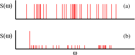
Figure 1: Parametrizations of the spectral function used in this work. In (a) a large number of $\delta$-functions with the same amplitude occupy frequencies $\omega_{i}$ in the continuum (or, in practice, on a very fine frequency grid). The locations are sampled in the SAC procedure. In (b), the $\delta$-function at the lowest frequency $\omega_{0}$ has a larger amplitude, $a_{0}>a_{i}$ for $i>0$, and this amplitude is optimized in the way described in the text. The frequencies of all the $\delta$-functions, including $\omega_{0}$, are sampled as in (a), but with the constraint $\omega_{0}<\omega_{i}~{}\forall~{}i>0$.

We parametrize the spectrum by a number $N_{\omega}$ of $\delta$-functions in the continuum, as illustrated in Fig. 1;

$$S(\omega)=\sum_{i=0}^{N_{\omega}-1}{a_{i}}\delta(\omega-\omega_{i}),$$ (11)

working with a normalized spectrum, so that

$$\sum_{i=0}^{N_{\omega}-1}{a_{i}}=1,$$ (12)

which corresponds to $G(0)=1$ in Eq. (4). The pre-normalized value of $G(0)$ is used as a factor in the final result. In sampling the spectrum, we never change the normalization, and $G(0)$ therefore is not included in the data set defining $\chi^{2}$ in Eq. (7). The covariance matrix, Eq. (5), is also computed with normalization to $G(0)=1$ for each bootstrap sample, which has a consequence that the individual statistical errors $\sigma_{i}\to 0$ for $\tau_{i}\to 0$, as discussed further in Appendix A.

In Fig. 1(a) the $\delta$-functions all have the same weight, $a_{i}=N^{-1}_{\omega}$, with $N_{\omega}$ typically ranging from $500$ to $2000$ in the calculations presented in this paper. The sampling corresponds to changing the locations (frequencies) $\omega_{i}$ of the $\delta$-functions, with the standard Metropolis probability used to accept or reject a change $\omega_{i}\to\omega_{i}+d$, with $d$ chosen at random within a window centered at $d=0$. The width of the window is adjusted to give an acceptance rate close to $1/2$. We collect the spectral weight in a histogram, averaging over sufficiently many updating cycles of the frequencies to obtain smooth results. In practice, in order to be able to use a precomputed kernel ${\rm e}^{-\omega_{j}\tau_{i}}$ in Eq. (4) for all times $\tau_{i}$ and frequencies $\omega_{j}$, we use a very fine grid of allowed frequencies (much finer than the histogram used for collecting the spectrum), e.g., with spacing $\Delta_{\omega}=10^{-5}$ in typical cases where the dominant spectral weight is roughly within the range $0-5$. We then also need to impose a maximum frequency, e.g., $\omega_{\rm max}=20$ under the above conditions. With $\approx 100$ $\tau$-values the amount of memory needed to store the kernel is then still reasonable, and in practice the fine grid produces results indistinguishable from ones obtained in the continuum (strictly speaking double-precision floating-point numbers) without limitation, i.e., without even an upper bound imposed on the frequencies.

We have found that not changing the amplitudes of the $\delta$-functions is an advantage in terms of the sampling time required to obtain good results, and there are other advantages as well, as will be discussed further in a forthcoming technical article shao17 . One can also initialize the amplitudes with a range of different weights (e.g., of the form $a_{i}\propto i^{\alpha}$, with $\alpha>0$), while maintaining the normalization Eq. (12). This modification of the scheme can help if the spectrum has a gap separating regions of significant spectral weight, since an additional amplitude-swap update, $a_{i}\leftrightarrow a_{j}$, can easily transfer weight between two separate regions when the weights are all different, thus speeding up the sampling (but we typically do not find significant differences in the final results as compared with all-equal $a_{i}$). This method was already applied to spectral functions of a 3D quantum critical antiferromagnet in Ref. qin17, . Here we do not have any indications of mid-spectrum gaps and use the constant-weight ensemble, however, with a crucial modification.

As illustrated in Fig. 1(b), in order to reproduce the kind of spectral function expected in the 2D Heisenberg model—a magnon pole followed by a continuum—we have developed a modified parametrization where we give special treatment to the $\delta$-function with lowest frequency $\omega_{0}$. We adjust its amplitude $a_{0}$ in a manner described further below but keep it fixed in the sampling of frequencies. The common amplitude for the other $\delta$-functions is then $a_{i}=(1-a_{0})/(N_{\omega}-1)$. The determination of the best $a_{0}$ value also relies on how the sampling temperature $\Theta$ is chosen, which we discuss next.

Consider first the case of all $\delta$-functions having equal amplitude; Fig. 1(a). As an initial step, we carry out a simulated annealing procedure with slowly decreasing $\Theta$ to find the lowest, or very close to the lowest, possible value of $\chi^{2}$ (which will never be exactly $0$, no matter how many $\delta$-functions are used, because of the positive-definiteness imposed on the spectrum). We then raise $\Theta$ to a value where the sampled mean value $\langle\chi^{2}\rangle$ of the goodness of fit is higher than the minimum value $\chi^{2}_{\rm min}$ by an amount of the order of the standard deviation of the $\chi^{2}$ distribution, i.e, going away from the overfitting region where the process becomes sensitive to the detrimental effects of the statistical errors (i.e., producing a nonphysical spectrum with a small number of sharp peaks). Considering the statistical expectation that the best fit should have $\chi^{2}_{\rm min}\approx N_{\rm dof}=N_{\tau}-N_{\rm para}$, where $N_{\rm para}$ is the (unknown) effective number of parameters of the spectrum and the minimum $\chi^{2}$ value can be taken as an estimate of the effective number of degrees of freedom; $\chi^{2}_{\rm min}\approx N_{\rm dof}$. Hence, the standard deviation $\sigma_{\chi^{2}}=(2N_{\rm dof})^{1/2}$ can be replaced by the statistically valid approximation

$$\sigma_{\chi^{2}}\approx\sqrt{2\chi^{2}_{\rm min}}.$$ (13)

Thus, we adjust $\Theta$ such that

$$\langle\chi^{2}\rangle\approx\chi^{2}_{\rm min}+a\sqrt{2\chi^{2}_{\rm min}},$$ (14)

with the constant $a$ of order one. For spectral functions with no sharp features, we find that this method with the parametrization in Fig. 1(a) produces good, stable results, with very little dependence of the average spectrum on $a$ as long as it is of order one. For $a\to 0$ the data become overfitted, leading eventually to a spectrum consisting of a small number of sharp peaks with little resemblance to the true spectrum.

Using the unrestricted sampling with the parametrization in Fig. 1(a), with QMC data of typical quality one cannot expect to resolve a very sharp peak—in the extreme case a $\delta$-function—because it will be washed out by entropy. Therefore, in most of the calculations reported in this paper we proceed in a different way in order to incorporate the expected $\delta$-function. After determining $\chi^{2}_{\rm min}$, we switch to the parametrization in Fig. 1(b), and the next step is to find an optimal value of the amplitude $a_{0}$. To this end we rely on the insight from Ref. sandvik16, that the optimal value of a parameter affecting the amount of configurational entropy in the spectrum can be determined by monitoring $\langle\chi^{2}\rangle$ as a function of that parameter at fixed sampling temperature $\Theta$. In the case of $a_{0}$, increasing its value will remove entropy from the spectrum. Since entropy is what tends to spread out the spectral weight excessively into regions where there should be little weight or no weight at all, a reduced entropy can be reflected in a smaller value of $\langle\chi^{2}\rangle$. Thus, in cases where the spectrum is gapped, a sampling with the parametrization in Fig. 1(a) will lead to spectral weight in the gap and an overall distorted spectrum. However, upon switching to the parametrization in Fig. 1(b) and gradually increasing $a_{0}$, no weight can appear below $\omega_{0}$ and $\langle\omega_{0}\rangle$ will gradually increase (and note again that $\omega_{0}$ is not fixed but is sampled along with the other frequencies $\omega_{i}$) because a good match with the QMC data $\{\bar{G}\}$ cannot be obtained if there is too much weight in the gap. In this process $\langle\chi^{2}\rangle$ will decrease. Upon increasing $a_{0}$ further, $\langle\omega_{0}\rangle$ will eventually be pushed too far above the gap, and then $\langle\chi^{2}\rangle$ clearly must start to increase. Thus, if there is a $\delta$-function at the lower edge of the spectrum pursued, one can in general expect a minimum in $\langle\chi^{2}\rangle$ versus $a_{0}$, and, if the QMC data are good enough, this minimum should be close to the true value of $a_{0}$. When fixing $a_{0}$ to its optimal value at the $\langle\chi^{2}\rangle$-minimum, the frequency $\omega_{0}$ should fluctuate around its correct value (with normally very small fluctuations so that the final result is a very sharp peak). If there is no such $\delta$-function in the true spectrum, one would expect the $\langle\chi^{2}\rangle$ minimum very close to $a_{0}=0$. Extensive testing, to be reported elsewhere shao17 , has confirmed this picture. We here show test results relevant to the type of spectral function expected for the 2D Heisenberg model.

One might think that we could also sample the weight $a_{0}$ instead of optimizing its fixed value. The reason why this does not work is at the heart of our approach: Including Monte Carlo updates changing the value of $a_{0}$ (and thus also of all other weights $a_{i>0}$ to maintain normalization), entropic pressures will favor values close to the other amplitudes and the results (which we have confirmed) are indistinguishable from those obtained without special treatment of the lower edge, i.e., the parametrization in Fig. 1(a). The entropy associated with different parametrizations will be further discussed in a separate article shao17 .

II.3 Tests on synthetic data

To test whether the method can resolve the kind of spectral features that are expected in the 2D Heisenberg model, we construct a synthetic spectral function with a $\delta$-function of weight $a_{0}$ and frequency $\omega_{0}$, followed by a continuum with total weight $1-a_{0}$. The relationship in Eq. (4) is used to obtain $G(\tau)$ for a set of $\tau$-points and normal-distributed noise is added to the $G$ values, with standard deviation typical in QMC results. To provide an even closer approximation to real QMC data, we construct correlated noise. Here one can adjust the autocorrelation time of the correlated noise to be close to what is observed in QMC data. The way we do this is discussed in more detail in Appendix A.

As we will discuss in Sec. III, for the 2D Heisenberg model we find that the smallest relative weight of the magnon pole is $\approx 0.4$ at ${\bf q}=(\pi,0)$. We therefore here test with $a_{0}=0.4$, set $\omega_{0}=1$ and take for the continuum a truncated Gaussian (with no weight below $\omega_{0}$) of width $\sigma=1$. This situation of no gap between the $\delta$-function and the continuum should be expected to be very challenging for any analytic continuation method. Extracting $a_{0}$ and $\omega_{0}$ by simply fitting an exponential $a_{0}{\rm e}^{-\omega_{0}\tau}$ to the QMC data for large $\tau$ is difficult because there will never be any purely exponential decay (unlike the case where there is a gap between the $\delta$-function and the continuum) and the best one could hope for is to extrapolate the parameters based on different ranges of $\tau$ included in the fit, or with some more sophisticated analysis suwa16 . As we will see below, with noise levels in the synthetic data similar to our real QMC data, the SAC procedure outlined above not only produces good results for $a_{0}$ and $\omega_{0}$ but also reproduces the continuum well.

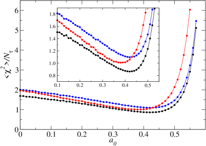
Figure 2: The goodness of the fit versus the amplitude $a_{0}$ of the lowest $\delta$-function in three runs with different noise realizations for a synthetic spectrum with a $\delta$-function of weight $a_{0}=0.4$ at $\omega_{0}=1$. The continuum is a Gaussian of width $1$ centered at the same $\omega_{0}$, with the weight below $\omega_{0}$ excluded. The noise level is $\sigma_{i}\approx 10^{-5}$ and the errors are correlated with autocorrelation time $1$ according to the description in Appendix A. The inset shows the data close to the $\langle\chi^{2}\rangle$ minimum on a different scale.

When looking for the minimum value of $\langle\chi^{2}\rangle$ versus $a_{0}$, it is better to start with a somewhat higher $\Theta$ than what is obtained with the $\chi^{2}$ criterion in Eq. (14), so that the minimum can be more pronounced. Staying in the regime where the fit can still be considered good and the effects on $S(\omega)$ of a slightly elevated $\Theta$ are very minor, we aim for $\langle\chi^{2}\rangle\approx\chi^{2}_{\rm min}+bN_{\tau}$ with $b=1$ or $2$ at the initial stage of fixing $\Theta$ without the special treatment of the lowest $\delta$-function. With the so obtained $\Theta$ we scan over $a_{0}$ with some step size $\Delta a_{0}$. The scan is terminated when $\langle\chi^{2}\rangle$ has increased well past its minimum. The $\langle\chi^{2}\rangle$ curve can be analyzed later to locate the optimal $a_{0}$ value. If all the spectra generated in the scan have been saved one can simply use the best one. Since $\langle\chi^{2}\rangle$ normally will be significantly smaller at the optimal value of $a_{0}$ than at the starting point with $a_{0}=0$, there is typically no need for further adjustments of $\Theta$ later, though one can also do a final run at the optimal $a_{0}$ with the criterion in Eq. (14).

Fig. 2 shows typical $\langle\chi^{2}\rangle$ behaviors in tests with spectrum consisting of a $\delta$-function and a continuum of relative size and width similar to what we will report for the Heisenberg model in the next section. Here we used $80$ $\tau$-points on a uniform grid with spacing $\Delta_{\tau}=0.1$ and noise level $\sigma_{i}\approx 10^{-5}$ for $\tau$ points sufficiently away from $\tau=0$. We built in covariance similar to what is observed in the QMC data (also discussed in Appendix A). We can indeed observe a clear minimum in the $\langle\chi^{2}\rangle$ curve close to the expected value $a_{0}=0.4$. The deviations from this point reflect the effects of the statistical errors. In several runs at much smaller noise level, $\sigma_{i}\approx 10^{-6}$, the minimum was always at $0.40$ in scans with $\Delta a_{0}=0.01$.

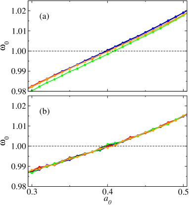
Figure 3: Mean value of $\omega_{0}$ in SAC runs with four different noise realizations (shown in different colors) graphed vs the amplitude parameter $a_{0}$. The noise level is $10^{-5}$ and $10^{-6}$ in (a) and (b), respectively, and the number of $\delta$-functions was $N_{\omega}=1000$ and $N_{\omega}=2000$. In both cases $G(\tau)$ values were generated on a uniform grid with $\Delta_{\tau}=0.1$ for $\tau$ up to the point where the relative error exceeds $10\%$.

The effects of the noise are smaller in the mean location $\langle\omega_{0}\rangle$ of the lowest $\delta$-function. Fig. 3 shows results versus $a_{0}$ from several different runs. At the correct value $a_{0}=0.4$, the error in the frequency is typically less than $10^{-3}$ at noise level $10^{-5}$ and smaller still at $10^{-6}$. Considering the uncertainty in the location of the minimum in Fig. 2, the total error on $\omega_{0}$ of course becomes higher, but still the precision is typically better than $10^{-2}$ for noise level $10^{-5}$ and much better at $10^{-6}$.

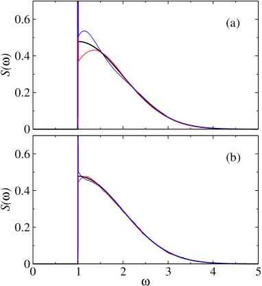
Figure 4: Two typical SAC-computed spectral functions (red and blue curves, obtained with different noise realizations) compared with the underlying true synthetic spectrum (thicker black curve, with the half-Gaussian containing $60\%$ of the weight). The parameters of the spectrum are the same as in Fig. 6. The noise level is $10^{-5}$ and $10^{-6}$ in (a) and (b), respectively.

The full SAC spectral functions at both noise levels are shown in Fig. 4, for two noise realizations in each case (with the spectra taken at their respective optimal $a_{0}$ values). When constructing the histogram for averaging the spectrum, here with a bin with $\Delta\omega=0.005$, we also include the main $\delta$-peak. If the fluctuations in $\omega_{0}$ are large, a broadened peak will result. Here the fluctuations are very small and no significant broadening is seen beyond that due to the histogram binning. As discussed above, the location of the main peak is very well reproduced. The continuum typically shows the strongest deviations from the correct curve close to the edge. The improvements when going from noise level $10^{-5}$ to $10^{-6}$ are obvious in the figure.

Statistical errors of order $10^{-5}$ in the correlation function $G(\tau)$ normalized to $1$ at $\tau=0$ are relatively easy to achieve in QMC calculations, and in many cases it is possible to go to $10^{-6}$ or even better. The tests here show that quite detailed information can be obtained with such data for spectral functions with a prominent $\delta$-function at the lower edge followed by a broad continuum. Importantly, the approach also involves the estimation of the statistical error on the weight of the $\delta$-function through a bootstrapping procedure, and based on tests such as those above, as well as additional cases, we do not see any signs of further systematical errors in the weight and location of the $\delta$-function, i.e., the method is unbiased in this regard. It is still of course not easy to discriminate between a spectrum with an extremely narrow peak and one with a true $\delta$-function, but a broad peak will manifest itself in the loss of amplitude $a_{0}$, accumulation of the “background” $\delta$-functions as a leading maximum at the edge, and in large fluctuations in the lower edge $\omega_{0}$. We therefore have good reasons to believe that the approach is suitable in general both for reproducing spectra with an extremely narrow peak and for detecting when such a peak is absent.

III Heisenberg model

In quantum magnetism the most important spectral function is the dynamic spin structure factor $S^{\alpha}({\bf q},\omega)$, corresponding to the correlations of the spin operator $S_{\bf q}^{\alpha}$ $(\alpha=x,y,z)$, the Fourier transform of the real-space spin operator $S_{\bf r}^{\alpha}$ as in Eq. (2). This spectral function is directly proportional to the inelastic neutron-scattering cross-section at wavevector transfer ${\bf q}$ and energy transfer $\omega$ formfactor . In this paper we focus on isotropic spin systems and do not break the symmetry in the finite-size calculations; thus all components $\alpha$ are the same, corresponding to the total cross-section averaged over the longitudinal and transverse channels (i.e., as obtained in experiments with unpolarized neutrons). We consider the $z$-component in the SSE-QMC calculations and hereafter use the notation $S({\bf q},\omega)$ without any $\alpha$ superscript. With sufficiently large inverse temperature, here $\beta=4L$ in most QMC simulations, we obtain ground-state properties for all practical purposes for ${\bf q}$ at which the gap $\omega_{\bf q}$ is sufficiently large. More precisely, we have well-converged data for all ${\bf q}$ except for ${\bf q}=(\pi,\pi)$, where the finite-size gap closes as $1/L^{2}$ (this being the lowest excitation in the Anderson tower of quantum-rotor states), much faster than the lowest magnon excitation which has a gap $\propto 1/L$. Therefore, in the following we do not analyze the not fully-converged ${\bf q}=(\pi,\pi)$ data. In addition to the QMC calculations, where we go up to linear system sizes $L=48$, we also report exact $T=0$ Lanczos ED results for lattices with up to $N=40$ spins.

For the square-lattice Heisenberg antiferromagnet, the spectral function in calculations such as conventional spinwave expansions Igarashi92 ; Canali93 ; Igarashi05 ; syromyatnikov10 and continuous unitary transformations (an approach which also starts from spinwave theory, formulated with the Dyson-Maleev representation of the spin operators) Powalski15 ; Powalski17 contains a dominant $\delta$-function at the lowest frequency $\omega_{\bf q}$ and a continuum above this frequency,

$$S({\bf q},\omega)=S_{0}({\bf q})\delta(\omega-\omega_{\bf q})+S_{c}({\bf q},\omega),$$ (15)

where $\omega_{\bf q}$ is also the single-magnon dispersion and $S_{0}({\bf q})$ is the spectral weight in the magnon pole. We define the relative weight of the single-magnon contribution as

$$a_{0}({\bf q})=\frac{S_{0}({\bf q})}{\int d\omega S({\bf q},\omega)},$$ (16)

in the same way as the generic $a_{0}$ in Sec. II.

In principle the single-magnon pole may be broadened, but the damping processes causing this are of very high order in the spinwave interaction terms and we are not aware of any calculations estimating these effects quantitatively. In general it is expected that the broadening of the magnon pole itself should be very small in bipartite (collinear AFM-ordered) Heisenberg systems chernyshev06 ; chernyshev09 . Accordingly, we can here make the simplifying assumption that there is no broadening at $T=0$ of the single-magnon pole itself, i.e., that interaction effects are manifested as spectral weight transferred from the $\delta$-function to the continuum above it. In contrast, in non-bipartite (frustrated) antiferromagnets with non-collinear order, there are other lower-order magnon damping mechanisms present that cause significant broadening of the $\delta$-function chernyshev06 ; chernyshev09 .

In a previous QMC calculation where the analytic continuation was carried out by function fitting including a $\delta$-function edge sandvik01 , the continuum $S_{c}({\bf q},\omega)$ was modeled with a specific functional form with a number of parameters (adjusted to fit the QMC data). Here we do not make any prior assumptions on the shape of the continuum, instead applying the SAC procedure with the parametrization illustrated in Fig. 1(b). If the $\delta$-function is actually substantially broadened, such that the separation of the spectrum into two distinct parts in Eq. (15) becomes inappropriate, we expect our SAC approach to simply give a very small amplitude $S_{0}({\bf q})$ when this is the case. We will see examples of this kind of full depletion of the magnon pole later in Sec. IV, where other interactions are added to the Heisenberg model (the $J$-$Q$ model). Later in this section we will also show some results for the Heisenberg model obtained without assuming a $\delta$-function in Eq. (15).

To briefly recapitulate the version of SAC we developed in Sec. II, after fixing a proper sampling temperature using the spectrum without special treatment of the leading $\Delta$-function, i.e., the parametrization of the dynamic structure factor illustrated in in Fig. 1(a), in the final stage of the sampling process we use the parametrization ofFig. 1(b). The amplitude of the leading $\delta$-function is optimized based on the entropic signal—a minimum in the mean goodness of the fit, $\langle\chi^{2}\rangle$. The location of this special $\delta$-function is sampled along with all the other “small” ones representing the continuum, and the spectral weight as a function of the frequency is collected in a histogram (here typically with bin size $\Delta\omega=0.005$). Thus, in the final averaged spectrum the magnon pole may be broadened by fluctuations in its location, but, as we will see below, the width is typically very narrow and for all practical purposes it remains a $\delta$-function contribution. Here the level of the statistical QMC errors, with the definitions discussed in Sec. II, is $10^{-5}$ or better (some raw data are shown in Appendix A). Extensive testing, exemplified in Fig. 4, demonstrates that the method is well capable of reproducing the type of spectral function of interest here to a good degree with this data quality. The number $N_{\omega}$ of $\delta$-functions required in the continuum in order to obtain well converged results depends on the quality of the QMC data. We have carried out tests with different $N_{\omega}$ and find good convergence of the results when $N_{\omega}\approx 500-1000$. The results presented below were obtained with $N_{\omega}=2000$.

III.1 Spectral functions at different wavevectors

For an overview, we first show the spectral function for the $L=48$ system with a color plot in Fig. 5, where the $x$-axis corresponds to the wavevector along a standard path in the BZ and the $y$-axis is the frequency $\omega$. The location of the magnon pole (the dispersion relation) is indicated, and for the continuum a color coding is used. We also show an upper spectral bound defined such that $95\%$ of the weight for each ${\bf q}$ falls between the two curves. Due to matrix-elements effects related to conservation of the magnetization ($S^{z}_{q=0}$) of the Heisenberg model, the total spectral weight vanishes as $q\to 0$ and it is seen in Fig. 5 to be small in a wide region around this point. Both the total weight and the low-energy scattering is maximized as ${\bf q}\to(\pi,\pi)$. As mentioned above, exactly at $(\pi,\pi)$ our calculations are not $T\to 0$ converged, and we therefore do not show any results for this case. The width in $\omega$ of the region in which $95\%$ of the weight is concentrated is seen to be almost independent on ${\bf q}$. However, since the total spectral weight for ${\bf q}$ close to $(\pi,\pi)$ is very large there is significant weight extending up to $\omega\approx 6$, while in other ${\bf q}$ regions the weight extends roughly up to $4.5-5$ [except close to $(0,0)$, where no significant weight can be discerned in the density plot with the color coding used].

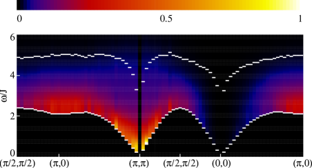
Figure 5: The dynamic structure factor of the 2D Heisenberg model computed on an $L=48$ lattice along the path in the BZ indicated on the $x$-axis. The $y$-axis is the energy transfer $\omega$ in units of the coupling $J$. The magnon peak ($\delta$-function) at the lower edge of the spectrum is marked in white irrespective of its weight, while the continuum is shown with color coding on an arbitrary scale where the highest value is $1$. The upper white curve corresponds to the location where, for given ${\bf q}$, $5\%$ of the spectral weight remains above it.

More detailed frequency profiles at four different wavevectors are shown in Fig. 6. In addition to the points $(\pi,0)$ and $(\pi/2,\pi/2)$, on which many prior works have focused, results for the points closest to the gapless points $(0,0)$ and $(\pi,\pi)$ are also shown. The results at $(\pi,0)$ and $(\pi/2,\pi/2)$ are in general in good agreement with the previous QMC calculations sandvik01 in which the $\delta$-function contributions were also explicitly included in the parametrization of the spectrum. The relative weight in the $\delta$-function, indicated in each panel in Fig. 6, is also in reasonably good agreement with series expansions around the Ising limit zheng05 . The relative spectral weight of the continuum, $1-a_{0}({\bf q})$, can be taken as a measure of the effect of spinwave interactions, which leads to the multi-magnon contributions often assumed to be responsible for the continuum. We will argue later that the particularly large continuum at $(\pi,0)$ is actually due to nearly deconfined spinons.

It is not clear whether the small maximum to the right of the $\delta$-function, which we see consistently through the BZ, are real spectral features or whether they reflect the statistical errors of the QMC data in a way similar to the most common distortion resulting from noisy synthetic data, as seen in the tests presented in Fig. 4. The error level of the QMC data in all cases is a bit below $10^{-5}$, i.e., similar to Fig. 4(a). The behavior does not suggest any gap between the $\delta$-functions and the continuum.

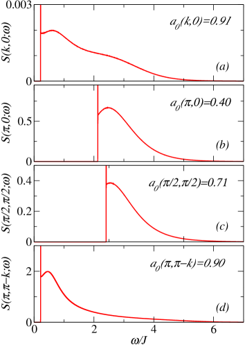
Figure 6: Dynamic structure factor for $L=48$ system at four different momenta. The smallest momentum increment $2\pi/L$ is denoted by $k$ in (a) and (d). The relative amplitude of the magnon pole is indicated in each panel.

III.2 Finite-size effects

It is important to investigate the size dependence of the spectral functions. For very small lattices at $T=0$, $S({\bf q},\omega)$ computed according to Eq. (1) for each ${\bf q}$ contains only a rather small number of $\delta$-functions and it is not possible to draw a curve approximating a smooth continuum following a leading $\delta$-functions. Therefore, the SAC procedure does not reproduce exact Lanczos results very well—we obtain a single broad continuum following the leading $\delta$-function, instead of several small peaks. Because the continuum also has weight close to the leading $\delta$-function, between it and the second peak of the actual spectrum, the SAC method also slightly underestimates the weight in the first $\delta$-function. If the continuum emerging as the system size increases indeed is, as expected, broad and does not exhibit any unresolvable fine-structure, the tests in Sec. II suggest that our methods should be able to reproduce it.

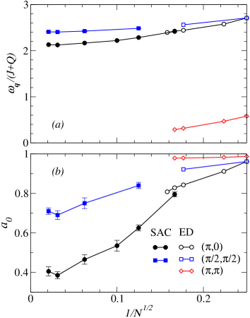
Figure 7: Size dependence of the single-magnon energy (a) and weight in the magnon pole (b) at wavevectors ${\bf q}=(\pi,0)$, $(\pi/2,\pi/2)$, and $(\pi,\pi)$. Lanczos ED results for small systems ($L\times L$ lattices with $L=4$ and $L=6$ as well as tilted lattices with $N=20,32$, and $40$ sites) are shown as open circles and QMC-SAC data are presented as solid circles with error bars. The error bars were estimated by bootstrap analysis (i.e., carrying out the SAC procedure multiple times with random samples of the QMC data bins).

For the $6\times 6$ lattice at ${\bf q}=(\pi,0)$, our SAC result underestimates the weight in the magnon pole by about $5\%$, while the energy deviates by less than $1\%$. We expect these systematic errors to decrease with increasing system size, for the reasons explained above. Fig. 7 shows the size dependence of the single-magnon weight and energy at wavevectors ${\bf q}=(\pi,0)$, $(\pi/2,\pi/2)$, and $(\pi,\pi)$. At $(\pi,\pi)$ we only have Lanczos results, but even with the small systems accessible with this method it can be seen that indeed the energy decays toward zero. The magnon weight is large, converging rapidly toward about $97\%$, which is similar to the series-expansion result zheng05 . The energies at ${\bf q}=(\pi,0)$ and $(\pi/2,\pi/2)$ also converge rapidly, with no detectable differences between $L=32$ and $L=48$, and a smooth transition between the ED results for small systems and QMC results for larger sizes. The magnon weight at these wavevectors show more substantial size dependence, though again the results for the two largest sizes agree within error bars. Here the connection between the ED and QMC results does not appear completely smooth at $(\pi,0)$, due to the difficulties for the SAC method to deal with a spectrum with a small number of $\delta$-functions. Nevertheless, even the ED results indicate a drop in the amplitude for the larger system sizes. The trends in $1/L$ for the QMC results suggest that the weight converges to slightly below $40\%$ at ${\bf q}=(\pi,0)$ and slightly below $70\%$ at ${\bf q}=(\pi/2,\pi/2)$, both in very good agreement with the series-expansion results zheng05 . This agreement with a completely different method provides strong support to the accuracy of the QMC-SAC procedures. The energies also agree very well with the previous QMC results where particular functional forms were used to model the continuum, and the magnon amplitudes agree within $5-10\%$ (with the values indicated in the insets of Fig. 3 in Ref. sandvik01, ).

III.3 Comparisons with experiments

In the discussion of the recent neutron-scattering experiments on CFTD piazza15 , it was argued that the large continuum in the $(\pi,0)$ spectrum is due to fully deconfined spinons, and a variational RVB wavefunction was used to support this interpretation. We will discuss our different picture of nearly deconfined spinons further in Sec. V. Here we first compare the $(\pi,0)$ and $(\pi/2,\pi/2)$ results with the experimental data without invoking any interpretation. The experimental scattering cross section in Ref. piazza15, was shown versus the frequency $\omega/J$ normalized by the estimated value of the coupling constant ($J\approx 6.11$ meV). Keeping the same scale, we should only convolute our spectral functions with an experimental Gaussian broadening. We optimize this broadening to match the data and find that a half-width $\sigma=0.12J$ of the Gaussian works well for both wavevectors—which is the same as the instrumental broadening reported for the experiment piazza15 . Since the neutron data are presented with an arbitrary scale for the scattering intensity we also have to multiply our $S({\bf q},\omega)$ for each ${\bf q}$ by a common factor. The agreement with the data at both $(\pi,0)$ and $(\pi/2,\pi/2)$ is very good, and can be further improved by dividing $\omega/J$ in the experimental data by $1.02$, which corresponds to $J\approx 6.23$ meV, which should still be within the errors of the experimentally estimated value. As shown in Fig. 8, the agreement with the experiments is not perfect but probably as good as could possibly be expected, considering small effects of the weakly ${\bf q}$-dependent form factor formfactor and some influence of weak interactions beyond $J$ (longer-range exchange, ring exchange, spin-phonon couplings, disorder, etc.).

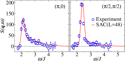
Figure 8: Comparison of the CFTD experimental data piazza15 (the full scattering cross section corresponding to unpolarized neutrons) and our QMC-SAC spectral functions at wavevectors ${\bf q}=(\pi,0)$ and ${\bf q}=(\pi/2,\pi/2)$. To account for experimental resolution, we have convoluted the QMC-SAC spectral functions in Figs. 6(b,c) with a common Gaussian broadening (half-width $\sigma=0.12J$). We have renormalized the exchange constant by a factor $1.02$ relative to the original value in Ref. piazza15, , and to match the arbitrary factor in the experimental data we have further multiplied both of our spectra by a factor $\approx 50$.

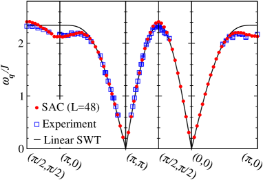
Figure 9: Single-magnon dispersion $\omega_{\bf q}$ along a representative path of the magnetic BZ. The CFTD experimental data from Ref. piazza15, are shown as blue squares and the QMC-SAC data (the location of the magnon pole) are shown with red circles. We also show the linear SWT dispersion (black curve) adjusted by a common factor corresponding to the exact spinwave velocity $c=1.65847$ sen15 .

The single-magnon dispersion, the energy $\omega_{\bf q}$ in Eq. (15), is compared with the corresponding experimental peak position in Fig. 9. The linear spinwave dispersion is shown as a reference, using the best available value of the renormalized velocity $c=1.65847$ sen15 . Our results agree very well with the spinwave dispersion at low energies, and with the experimental CDFT data piazza15 also in the high-energy regions where the spinwave results are not applicable. The only statistically significant deviation, though rather small, is at ${\bf q}\approx(\pi/2,\pi/2)$, where the experimental energy is lower (as seen also in the peak location in Fig. 8). Still, overall, one must conclude that CFTD is an excellent realization of the square-lattice Heisenberg model at the level of current state-of-the-art experiments. It would certainly be interesting to improve the frequency resolution further and try to analyze higher-order effects, which should become possible in future neutron scattering experiments.

III.4 Wavevector dependence of the single-magnon amplitude

We next look at the variation of the relative magnon weight $a_{0}({\bf q})$ along the representative path of the BZ for $L=48$, shown in Fig. 10. For ${\bf q}\to(0,0)$ and $(\pi,\pi)$ the weight $a_{0}$ increases and appears to tend close to $1$. From the results exactly at $(\pi,\pi)$ in Fig. 7 we know that in this case the remaining weight in the continuum should be about $3\%$, which is also in good agreement with the series results in Ref. zheng05, , where a similar non-zero multi-magnon weight was also found as $q\to 0$. At ${\bf q}=(\pi/2,\pi/2)$, as also shown in Fig. 7, the magnon pole contains about $70\%$ of the weight, while at ${\bf q}=(\pi,0)$ this weight is reduced to about $40\%$. Both of these are also in good agreement with Ref. zheng05, , and in fact throughout the BZ path we find no significant deviations from the series results. This again reaffirms the ability of the SAC procedure to correctly optimize the amplitude of the leading $\delta$-function. It should be noted that the series expansion around the Ising model does not produce the full spectral functions, only the single-magnon dispersion and weight.

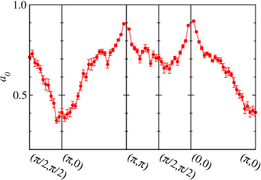
Figure 10: Relative spectral weight of the single-magnon pole along the representative path in the BZ for the $L=48$ Heisenberg system. Error bars were estimated by bootstrapping.

The depletion seen in Fig. 10 of the single-magnon weight in a neighborhood of ${\bf q}=(\pi,0)$ can also be related to the experimental data for CFTD. In Fig. 1(a) of Ref. piazza15, , a color coding is used for the scattering intensity such that even a modest reduction in the coherent single-magnon weight has a large visual impact. The region in which the spectral function is smeared out with no sharp feature in this representation corresponds closely to the region where the single-magnon weight drops from about $60\%$ to $40\%$ in our Fig. 10.

III.5 Alternative ways of analytic continuation

One could of course argue that the existence of the magnon pole at $(\pi,0)$ is not proven by our calculations since it has been built into our parametrization of the spectral function. While it is clear that our approach cannot distinguish between a very narrow peak and a $\delta$-function, if the broadening is significant for some ${\bf q}$, so that the main peak essentially becomes part of the continuum, we would expect the optimal amplitude $a_{0}({\bf q})$ to be very small or vanish. Nevertheless, to explore the possibility of spectra without magnon pole, we also have carried out the analytic continuation in two alternative ways, using the parametrization in Fig. 1(a) without special treatment of the lowest frequency, or by imposing a lower frequency bound.

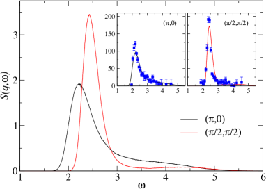
Figure 11: Spectral functions at ${\bf q}=(\pi,0)$ and $(\pi/2,\pi/2)$ obtained using unconstrained SAC with the parametrization in Fig. 1(a). The insets show comparisons with the experimental data piazza15 , where we have only adjusted a common amplitude to match the areas under the peaks.

Sampling without any constraints with $N_{\omega}=1000$ $\delta$-functions gives the results at $q=(\pi,0)$ and $(\pi/2,\pi/2)$ shown in Fig. 11. Here one can distinguish a peak in each case in the general neighborhood of where the $\delta$-function is located in Figs. 6(b,c), with the the maximum shifted slightly to higher frequencies and weight extending significantly to lower frequencies. At ${\bf q}=(\pi/2,\pi/2)$ there is now a shallow minimum before a low broad distribution at higher energies. This kind of behavior is typical for analytic continuation methods when there is too much broadening at low frequency, which leads to a compensating (in order to match the QMC data) depletion of weight above the main peak. Similarly, the up-shift of the location of the peak frequency at both q relative to Fig. 6 is due to there being weight also at $\omega<\omega_{\bf q}$ where there should be none or much less weight. In the insets of Fig. 11 we show comparisons with the CFTD experimental data. Here the SAC spectral functions are broader than the experimental profiles and we have not applied any additional broadening. It is clear that the SAC results here do not match the experiments as well as in Fig. 8, most likely because the QMC data are no sufficiently precise to reproduce a narrow magnon pole, thus also leading to other distortions at higher energy.

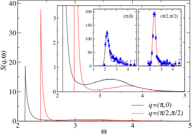
Figure 12: Spectral functions obtained using sampling with the parametrization in Fig. 1(a) under the constraint that no weight falls below the lower bounds determined with a $\delta$-function at the lower edge (Fig. 6); $\omega_{q}=2.13$ and $2.40$ for ${\bf q}=(\pi,0)$ and $(\pi/2,\pi/2)$, respectively. The inset shows the results on a different scale to make the continua better visible. The insets of the inset show comparisons with the experimental data, where we have broadened the numerical results by Gaussian convolution and adjusted a common amplitude.

In order to reduce the broadening and other distortions arising as a consequence of spectral weight spreading out in the SAC sampling procedure due to entropic pressure sandvik16 into regions where there should be no weight, we also carried out SAC runs with the constraint that no $\delta$-function can go below the lowest energy determined with the dominant $\delta$-function present. These energies, $\omega_{q}=2.13$ and $2.40$ for ${\bf q}=(\pi,0)$ and $(\pi/2,\pi/2)$, respectively, are in excellent agreement with the series expansions around the Ising limit zheng05 and, in the case of $(\pi/2,\pi/2)$, also with the well-converged high-order spin-wave expansion Igarashi92 ; Canali93 ; Igarashi05 ; syromyatnikov10 . There is therefore good reason to trust these as being close to the actual energies. As seen in Fig. 12, there is a dramatic effect of imposing the lower bound—the main peak is much higher and narrower than in Fig. 11 and an edge is formed at $\omega_{q}$. Most likely the peaks are still broadened on the right side, and again this broadening has as a consequence a local minimum in spectral weight before a broad second peak, which is now seen for both ${\bf q}$ points. In this case the comparisons with the experiments (insets of Fig. 12) is overall somewhat better than with the completely unconstrained sampling in Fig. 11, but still we see signs of a depletion of spectral weight to the right of the main peak that is not present in the experimental data. We take the $\omega_{0}$-constrained spectra as upper limits in terms of the widths of the main magnon peaks, and most likely the true spectra are much closer to those obtained with the optimized $\delta$-functions in Fig. 6.

In summary, the results of these alternative ways of carrying out the SAC process reaffirm that there indeed should be a leading very narrow magnon pole, close to a $\delta$-function, at both ${\bf q}=(\pi,0)$ and $(\pi/2,\pi/2)$. While the pole strictly speaking may have some damping, our good fits with a pure $\delta$-function in Fig. 8 indicates that such damping should be extremely weak, as also expected on theoretical grounds chernyshev06 ; chernyshev09 .

IV J-Q model

The AFM order parameter in the ground state of the Heisenberg model is significantly reduced by zero-point quantum fluctuations from its classical value $m_{s}=1/2$ to about $0.307$ Reger88 ; sandvik10a . It can be further reduced when frustrated interactions are included, eventually leading to a quantum-phase transition into a non-magnetic state, e.g., in the frustrated $J_{1}$-$J_{2}$ Heisenberg model dagotto89 ; gelfand89 ; hu13 ; gong14 ; morita15 ; wang17 . In the $J-Q$ model sandvik07 , the quantum phase transition driven by the four-spin coupling $Q$ appears to be a realization of the deconfined quantum critical point shao16 , which separates the AFM state and a spontaneously dimerized ground state; a columnar VBS. The model is amenable to large-scale QMC simulations and we consider it here in order to investigate the evolution of the dynamic structure factor upon reduction of the AFM order and approaching spinon deconfinement.

The $J$-$Q$ Hamiltonian can be written as sandvik07 ,

$$H=-J\sum_{\langle ij\rangle}P_{ij}-Q\sum_{\langle ijkl\rangle}P_{ij}P_{kl},$$ (17)

where $P_{ij}$ is a singlet projector on sites $ij$,

$$P_{ij}=1/4-{\bf S}_{i}\cdot{\bf S}_{j},$$ (18)

here on the nearest-neighbor sites. In the four-spin interaction $Q$ the site pairs $ij$ and $kl$ form horizontal and vertical edges of $2\times 2$ plaquettes. All translations and $90^{\circ}$ rotation of the operators are included in Eq. (17) so that all the symmetries of the square lattice are preserved.

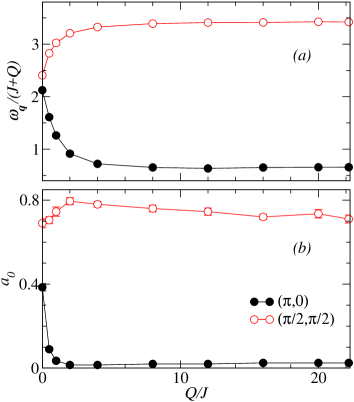
Figure 13: Results for the $J$-$Q$ model at ${\bf q}=(\pi,0)$ and $(\pi/2,\pi/2)$, calculated on the $L=32$ lattice. The lowest excitation energy $\omega_{q}$ (a) and the relative weight of the single-magnon contribution (b) are shown as functions of the coupling ratio $Q/J$ from the Heisenberg limit ($Q/J=0$) to the deconfined quantum critical point ($Q_{c}/J\approx 22$).

In addition to strong numerical evidence of a continuous AFM–VBS transition in the $J$-$Q$ model (most recently in Ref. shao16, ), there are also results pointing directly to spinon excitations at the critical point, in accord with the scenario of deconfined quantum criticality senthil04a ; senthil04b (where, strictly speaking, there may be weak residual spinon-spinon interactions, though those may only be important in practice only at very low energies tang13 ). Moreover, the set of gapless points is expanded from just the points ${\bf q}=(0,0)$ and $(\pi,\pi)$ in the Néel state to also ${\bf q}=(\pi,0)$ and $(0,\pi)$ spanu06 ; suwa16 at the critical point. Recent results point to linearly dispersing spinons with a common velocity around all the gapless points suwa16 .

Here our primary aim is to study how the magnon poles and continua in $S({\bf q},\omega)$ at ${\bf q}=(\pi,0)$ and $(\pi/2,\pi/2)$ evolve as the coupling ratio $Q/J$ is increased. We use the same SAC parametrization as in the previous section, with a leading $\delta$-function whose amplitude is optimized by finding the minimum in $\langle\chi^{2}\rangle$ versus $a_{0}({\bf q})$. We first consider the $L=32$ lattice and show our results for the energy and the relative amplitude in Fig. 13 as functions of the coupling ratio $Q/J$ all the way from the Heisenberg limit to the deconfined quantum critical point. Here the most notable aspect is the rapid drop in the magnon weight at ${\bf q}=(\pi,0)$, even for small values of $Q/J$, while at ${\bf q}=(\pi/2,\pi/2)$ the weight stays large, $70-80\%$, over the entire range. The energies depend on the normalization and here we have chosen $J+Q$ as the unit. We know from past work that the ${\bf q}=(\pi,0)$ energy at $Q_{c}/J$ vanishes in the thermodynamic limit but the reduction in the finite-size gap with the system size is rather slow suwa16 , and for the $L=32$ lattice considered here we are still far from the gapless behavior.

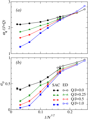
Figure 14: Size dependence of the excitation energy $\omega_{\bf q}$ (a) and the relative weight of the magnon pole $a_{0}({\bf q})$ (b) at ${\bf q}=(\pi,0)$ close to the Heisenberg limit of the $J$-$Q$ model.

We focus on the effects on small $Q$, where reliable extrapolations to infinite size are possible, and show the size dependence of the lowest excitation energy and the magnon amplitude at ${\bf q}=(\pi,0)$ for several cases in Fig. 14. We again show Lanczos ED results for small systems and QMC-SAC results for larger sizes. For the only common system size, $L=6$, the energies agree very well, as in the pure Heisenberg case discussed in the previous section, while the QMC-SAC calculations underestimate the magnon weight by a few percent due to the inability to resolve the details of a spectrum consisting of just a small number of $\delta$-functions. The most interesting feature is the dramatic reduction in the magnon weight even for very small ratios $Q/J$. For $Q/J=0.25$ and $0.5$, the size dependence indicates small remaining magnon poles, while at $Q/J=1$ it appears that the $\delta$-function completely vanishes in the thermodynamic limit.

In Fig. 15 we show the full ${\bf q}=(\pi,0)$ dynamic structure factor at $Q/J=4$, obtained with both the parametrizations in Fig. 1. The optimal weight of the leading $\delta$-function is only $1.4\%$ for this $L=32$ lattice, and the finite-size behavior indicates that no magnon pole at all should be present in the thermodynamic limit in this case. When no leading $\delta$-function is included in the SAC treatment, i.e., with unrestricted SAC sampling with the parametrization in Fig. 1(a), there is a little shoulder close to where the $\delta$-function is located with the other parametrization. The differences at higher frequencies are very minor. This is very different from the large change in the entire spectrum when unrestricted sampling is used for the same wavevector in the pure Heisenberg model, Fig. 11, which is clearly because of the much larger magnon pole in the latter case. This comparison also reinforces the ability of our SAC method to extract the correct weight of the leading $\delta$-function.

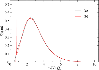
Figure 15: The ${\bf q}=(\pi,0)$ dynamic structure factor of the $J$-$Q$ model at $Q/J=4$ obtained using SAC with the two parametrizations of the the spectrum in Figs. 1(a,b). The relative weight of the leading $\delta$-function in (b) is $1.4\%$.

These results for the $J$-$Q$ model show that the magnon picture at $q=(\pi,0)$ fails even with a rather weak deformation of the Heisenberg model. Thus, it seems likely that the reduced excitation energy and coherent single-magnon weight at $q=(\pi,0)$, observed in the Heisenberg model as well as experimentally in CFTD, is a precursor to deconfined quantum criticality. If that is indeed the case, then it may be possible not only to describe the continuum in $S({\bf q},\omega)$ around ${\bf q}=(\pi,0)$ in terms of spinons piazza15 , but also to characterize the influence of spinons on the remaining sharp magnon pole. We next consider a simple effective Hamiltonian to address this possibility.

V Nature of the excitations

Motivated by the numerical results presented in Secs. III and IV, we here propose a mechanism of the excitations in the square-lattice Heisenberg model where the magnons have an internal structure corresponding to a mixing with spinons at higher energy. Our physical picture is that the magnon resonates in and out of the spinon space, which, in the absence of spinon-magnon couplings, exists above the bare magnon energy. We will construct a simple effective coupled magnon-spinon model describing such a mechanism. The model resembles the simplest model for the exciton-polariton problem, where the mixing is between light and a bound electron-hole pair (exciton). Here a bare photon can be absorbed by generating an exciton, and subsequently the electron and hole can recombine and emit a photon. This resulting collective resonating electron-hole-photon state is called an exciton-polariton hopfield58 ; mahan . The spinon-magnon model introduced here is more complex, because the magnon interacts not just with a single bound state but with a whole continuum of spinon states with or without (depending on model parameters) spinon-spinon interactions.

We start below by discussing the dispersion relations of the bare magnon and spinons, and then present details of the mixing process and the effective Hamiltonian. We will show that the model can reproduce the salient spectral features found for the Heisenberg and $J$-$Q$ models in the preceding section, in particular the differences between wavevectors $(\pi,0)$ and $(\pi/2,\pi/2)$ and the evolution of the spectral features when the $Q$ interaction is turned on, which in the effective model corresponds to lowering the bare spinon energy.

V.1 Effective Hamiltonian

In spinwave theory, the excitations of the square-lattice Heisenberg antiferromagnet are described as magnons, which to order $1/S$ disperse according to

$$\omega^{\text{m}}({\bf q})=c^{\text{m}}\sqrt{2-\frac{1}{2}\left[\cos(q_{x})+\cos(q_{y})\right]^{2}},$$ (19)

where $c^{\text{m}}$ is the spin wave velocity (the value of which is $c^{\text{m}}=1.637412$ when calculated to this order). We will take this form of $\omega^{\text{m}}({\bf q})$ as the bare magnon energy in our model but treat the velocity as an adjustable bare parameter.

Spinons are well understood in the $S=1/2$ AFM Heisenberg chain, where the dispersion relation is faddeev81 ; moller81

$$\omega(k)=\frac{\pi}{2}\sin(k),$$ (20)

and an $S=1$ excitation with wavenumber ${q}$ can exist at all energies $\omega({k}_{1})+\omega({k}_{2})$ with ${k}_{1}+{k}_{2}={q}$. In 2D, we use as input results of a recent QMC study of the excitation spectrum at the deconfined quantum critical point of the J-Q model suwa16 , where four gapless points at ${\bf q}=(0,0),(\pi,0),(0,\pi)$, and $(\pi,\pi)$ were found in the $S=1$ excitation spectrum (confirming a general expectation of a system at a continuous AFM–VBS transition spanu06 ). This dispersion relation is interpreted as the lower bound of a two-spinon continuum, which should also be the dispersion relation for a single spinon. In the effective model we will use the simplest spinon dispersion relation with the above four gapless points and shape in general agreement with the findings in Ref. suwa16, ,

$$\omega^{\text{s}}({\bf q})=c^{\text{s}}\sqrt{1-\cos^{2}(q_{x})\cos^{2}(q_{y})},$$ (21)

which can also be regarded as a 2D generalization of the 1D spinon dispersion, Eq. (20). The common velocity $c^{\text{s}}$ at the gapless points was determined for the critical $J$-$Q$ model suwa16 but here we will regard it as a free parameter.

One of our basic assumptions will be that spinons exist in the system also in the AFM phase, but they are no longer gapless and interact with the magnon excitations. We will add a constant $\Delta$ to the spinon energy Eq. (21) to model the evolution of the bare spinon dispersion from completely above the magnon energy $\omega^{\text{m}}({\bf q})$ at all ${\bf q}$ deep in the AFM phase to gradually approaching $\omega^{\text{m}}({\bf q})$ and eventually dipping below the magnon in parts of the BZ—which happens first at ${\bf q}=(\pi,0)$—as the AFM order is reduced. For two spinons, with one of them at wavevector ${\bf p}$ and the total wavevector being ${\bf q}$, the bare energy of the spinon pair is then,

$$\tilde{\omega}^{\text{s}}({\bf q,p}) = 2\Delta+c^{\text{s}}\sqrt{1-\cos^{2}(p_{x})\cos^{2}(p_{y})}$$

$$+ c^{\text{s}}\sqrt{1-\cos^{2}(q_{x}-p_{x})\cos^{2}(q_{y}-p_{y})}.$$

Here it should be noted that, in the simple picture of spinons in the basis of bipartite valence bonds, an $S=1$ excitation corresponds to breaking a valence bond (singlet), thereby creating a triplet of two spins, one in each of the sublattice A and B tang13 . The unpaired spins are always confined to their respective sublattices. There are also two species of magnons, and creating one of them corresponds to a change in magnetization by $\Delta S^{z}=1$ or $\Delta S^{z}=-1$, depending on the sublattice. Since $S^{z}$ must be conserved, we only need to consider one species of the magnons (e.g, $\Delta S^{z}=1$, which we associate with sublattice A) and that dictates the magnetization of the spinon pair that it can resonate with.

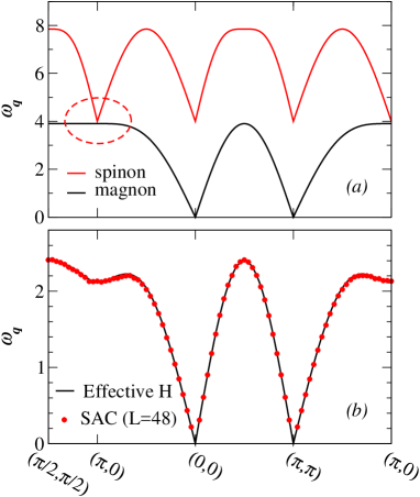
Figure 16: (a) Dispersions of the bare excitations of the effective model along a path through the BZ. The lower branch is for the magnon, and the upper branch is for a single spinon. The latter is also the lower edge of the two-spinon continuum. In this example, the spinons in the circled region close to ${\bf q}=(\pi,0)$ almost touch the magnon band, leading to significant spinon-magnon mixing. (b) The black curve shows the lowest energy of the mixed spinon-magnon system obtained with the dispersions in (a) and strength $g=5.1$ of the mixing term. The red circles show the results of the QMC-SAC calculations for the Heisenberg model on the $L=48$ lattice from Sec. III.

Instead of adding twice the gap as we do in Eq. (V.1), we could include $\Delta^{2}$ under each of the square-roots. This would cause some rounding of the V-shapes of the spinon dispersion. We have confirmed that there are no significant differences between the two ways of lifting the spinon energies in the coupled spinon-magnon system.

Using second-quantized notation, the non-interacting effective Hamiltonian in the space spanning single-magnon and spinon pair excitations can be written as

$$H^{\text{eff}-0}_{A}=\sum_{{\bf q}}\omega^{\text{m}}({\bf q})d^{\dagger}_{A,{\bf q}}d_{A,{\bf q}}$$

$$+\sum_{\bf q,p}\tilde{\omega}^{\text{s}}({\bf q,p})c^{\dagger}_{A,{\bf p}}c^{\dagger}_{B,{\bf q-p}}c_{A,{\bf p}}c_{B,{\bf q-p}}$$ (23)

where $c^{\dagger}$ ($c)$ and $d^{\dagger}$ ($d$) are the spinon and magnon creation (annihilation) operators, respectively, and there is also an implicit constraint on the Hilbert space to states with either a single magnon (here on the A sublattice) or two spinons (one on each sublattice). Note that both kinds of particles are bosons based on the broken-valence-bond picture of the spinons tang13 . For brevity of the notation we will hereafter drop the sublattice index, but in the calculations we always treat the two spinons as distinguishable particles.

Fig. 16(a) shows an example of the spinon and magnon dispersions corresponding to the situation we posit for the Heisenberg model. Here the spinon offset $\Delta$ is sufficiently large to push the entire two-spinon continuum (of which we only show the lower edge) up above the magnon energy, but at $(\pi,0)$ the spinons almost touch the magnon band. It is clear that any resonance process between the magnon and spinon Hilbert spaces will be most effective at this point, thus reducing the energy and accounting for the dip in the dispersion found in the QMC study of the Heisenberg model. In Fig. 16(b) we show how well the dispersion relation can be reproduced by the effective model, using a simple spinon-magnon mixing term that we will specify next.

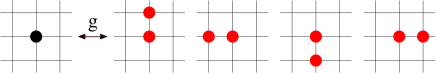
Figure 17: Illustration of the mixing process between the magnon (black circle) and the spinon pair (red circles). With mixing strength $g$, a magnon on a given sublattice splits up into a spinon pair occupying nearest-neighbor sites. The spinon pair can recombine and form a magnon on the original sublattice.

Our basic premise is that the magnon and spinon subspaces mix, through processes where a magnon is split into two spinons and vice versa. We use the simplest form of this mechanism, where the two spinons are created on neighboring sites, one of those sites being the one on which the magnon is destroyed. The interaction Hamiltonian in real space is

$$H^{\text{I}}=g\sum_{\bf r,\bf{e}}(c^{\dagger}_{\bf r+\bf{e}}c^{\dagger}_{\bf r}d_{\bf r}+d_{\bf r}^{\dagger}c_{\bf r}c_{{\bf r}+\bf{e}}),$$ (24)

where ${\bf e}$ denotes the four unit lattice vectors as illustrated in Fig. 17. In motivating this interaction, we have in mind how an $S=1$ excitation is created locally, e.g., in a neutron scattering experiment, by flipping a single spin. Spinwave theory describes the eigenstates of such excitations in momentum space and this leads to the bare magnon dispersion. A spinon in one dimension can be regarded as a point-like domain wall, and as such is associated with a lattice link instead of a site. However, in the valence bond basis, the spinons arise from broken bonds and are associated with sites (in any number of dimensions) tang13 . In this basis, the initial creation of the magnon also corresponds to creating two unpared spins, and the distinction between a magnon and two deconfined spinons only becomes clear when examining the nature of the eigenstates (where the spinons may or may not be well-defined particles, and they can be confined or deconfined). In the actual spin system, the magnon and spinons in the sense proposed here would never exist as independent particles (not even in any known limit), but the simplified coupled system can still provide a good description of the true excitations at the phenomenological level, as was also pointed out in the proposal of the AF* state (which also hosts topological order that is not present within our proposal) balents99 . Our way of coupling the two idealized bare systems according to Eq. (24) is intended as a simplest, local description of the mixing of the two posited parts of the Hilbert space. In the end, beyond its compelling physical picture with key ingredients taken from deconfined quantum criticality and the AF* state, the justification of the effective model will come from its ability to reproduce the key properties of the excitations of the Heisenberg model.

The magnon-spinon coupling in reciprocal space is

$$H^{\text{I}}=\sum_{{\bf q},{\bf p}}I({\bf p})(c_{\bf p}^{\dagger}c^{\dagger}_{{\bf q}-{\bf p}}d_{\bf q}+{\rm h.c.}),$$ (25)

where ${\bf q}$ again is the conserved total momentum and ${\bf p}$ is the momentum of the $A$ spinon (more precisely, the above spinon pair creation operator is $c_{A,\bf p}^{\dagger}c^{\dagger}_{B,{\bf q}-{\bf p}}$), and the form factor corresponding to the mixing strength $g$ in real space is

$$I({\bf p})=g\sqrt{\frac{2}{N}}\left[\cos(p_{x})+\cos(p_{y})\right].$$ (26)

If this interaction is used directly in a Hamiltonian with the bare magnon and spinon dispersions, we encounter the problem that the ground state is unstable—the mixing term will push the energy of the lowest excitations below that of the vacuum because the magnon mixes with the spinon and reduces its energy also at the gapless points. This behavior is analogous to what would happen to the exciton-polariton spectrum by including the light-matter interaction without the diamagnetic term. In reality, since $p^{2}\to(\mathbf{p}-q{\bf A})^{2}$, the minimal exciton-photon coupling is also responsible for a modification of the photon Hamiltonian, in a way which preserves the gapless spectrum hopfield58 ; mahan . Following the analogy between magnons/spinon-pairs and photons/excitons, we consider the coupling to arise from a modified spinon-pair operators by the following substitution in Eq. (23):

$$c^{\dagger}_{{\bf p}}c^{\dagger}_{{\bf q-p}}\to c^{\dagger}_{{\bf p}}c^{\dagger}_{{\bf q-p}}+G({\bf q,p})d^{\dagger}_{{\bf q}},$$ (27)

where the mixing function is given by:

$$G({\bf q,p})=\frac{I({\bf p})}{\tilde{\omega}^{\text{s}}({\bf q,p})}.$$ (28)

This substitution generates the following effective magnon-spinon Hamiltonian:

$$H^{\text{eff}}=\sum_{{\bf q}}\left(\omega^{\text{m}}({\bf q})+\sum_{\bf p}\tilde{\omega}^{\text{s}}({\bf q,p})G^{2}({\bf q,p})\right)d^{\dagger}_{{\bf q}}d_{{\bf q}}$$ (29)

$$+\sum_{{\bf p},{\bf q}}\left[\tilde{\omega}^{\text{s}}({\bf q,p})c^{\dagger}_{{\bf p}}c^{\dagger}_{{\bf q-p}}c_{{\bf p}}c_{{\bf q-p}}+I({\bf p})c_{\bf p}^{\dagger}c^{\dagger}_{{\bf q}-{\bf p}}d_{\bf q}+{\rm h.c.}\right],$$

Here we see explicitly how the interaction also affects the magnon dispersion (similar to the effect of the diamagnetic term on the exciton-polariton problem), so that the dressed magnons acquire a slightly renormalized velocity. This procedure guarantees that the ground state is stable and that the full spectrum of the coupled system is still gapless.

Some aspects of the observed behaviors in the Heisenberg and $J$-$Q$ models can be better reproduced if we also introduce a spinon-spinon interaction term $V$, to be specified later. Defining the modified magnon dispersion

$$\tilde{\omega}^{\text{m}}({\bf q})=\omega^{\text{m}}({\bf q})+\sum_{\bf p}\tilde{\omega}^{\text{s}}({\bf q,p})G^{2}({\bf q,p}),$$ (30)

the Hamiltonian in the sector of given total momentum ${\bf q}$ can be written as

$$H^{\text{eff}}({\bf q})=\tilde{\omega}^{\text{m}}({\bf q})d^{\dagger}_{{\bf q}}d_{{\bf q}}+\sum_{{\bf k},{\bf p}}V({\bf k},{\bf p})c^{\dagger}_{{\bf k}}c_{{\bf p}}c^{\dagger}_{{\bf q-k}}c_{{\bf q-p}}$$

$$+\sum_{\bf p}\left[\tilde{\omega}^{\text{s}}({\bf q,p})c^{\dagger}_{{\bf p}}c^{\dagger}_{{\bf q-p}}c_{{\bf p}}c_{{\bf q-p}}+I({\bf p})c_{\bf p}^{\dagger}c^{\dagger}_{{\bf q}-{\bf p}}d_{\bf q}+{\rm h.c.}\right].$$

(31)

Here it should be noted that, if spinon-spinon interactions are present, $V\not=0$, the definition of the function $G$ changes from Eq. (28) in the following simple way: the non-interacting two-spinon energies $\tilde{\omega}^{\text{s}}({\bf q,p})$ should be replaced by the eigenenergies of the interacting 2-spinon subsystem, and the momentum label ${\bf p}$ accordingly changes to a different index labeling the eigenstates. The mixing term is also transformed accordingly by using the proper basis in Eq. (27).

We study the effective Hamiltonian by numerical ED on $L\times L$ lattices with $L$ up to $64$. Our effective model is clearly very simplified and one should of course not expect it to provide a fully quantitative description of the excitations of the many-body spin Hamiltonians. Nevertheless, it is interesting that the parameters $c^{m},c^{s},\Delta,$ and $g$ can be chosen such that an almost perfect agreement with the Heisenberg magnon dispersion obtained in Sec. III is reproduced, as shown in Fig. 16(b) (where no spinon-spinon interactions are included). In the following we will not attempt to make any further detailed fits to the results for the spin systems, but focus on the general behaviors of the model and how they can be related to the salient features of the Heisenberg and $J$-$Q$ spectral functions.

V.2 Mixing states and spectral functions

For a given total momentum ${\bf q}$, the eigenstates $|n,{\bf q}\rangle$ of the effective Hamiltonian in Eq. (31) have overlaps $\langle n,{\bf q}|{\bf q}\rangle$ with the bare magnon state $|{\bf q}\rangle$. Without spinon-spinon interactions ($V=0$), with the bare spinons above the magnon band for all ${\bf q}$, and when the mixing parameter $g$ is suitable for describing the Heisenberg model [i.e., giving good agreement with the QMC dispersion relation, as in Fig. 16(b)], we find that all but the first and the last of these overlaps become very small when the lattice size $L$ increases. Thus, the two particular states are magnon-spinon resonances and the rest are essentially free states of the two-spinons. When attractive spinon-spinon interactions are included, the picture changes qualitatively, with the magnon also mixing in strongly with all spinon bound states. An example of spinon levels in the presence of spin-spin interactions are shown in Fig. 18, where a number of bound states separated by gaps can be distinguished. The stronger mixing with the bound states is simply a reflection of the fact that two bound spinons have a finite probability to occupy nearest-neighbor sites, so that the mixing process with the magnon (Fig. 17) can take place, while the probability of this vanishes when $L\to\infty$ for free spinons. Note that the total overlap $\langle n,{\bf q}|{\bf q}\rangle$ summed over all free-spinon states can still be non-zero, due to the increasing number of these states.

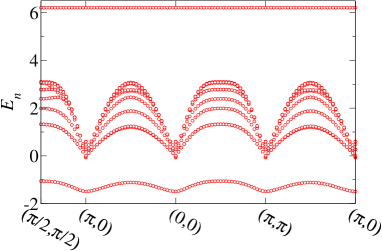
Figure 18: Energy levels versus the total wavevector of two spinons interacting through a potential $V(r)=-6.2{\rm e}^{-r/2}$. The bare dispersion relation of the single spinon is given by Eq. (21) with $c^{s}=3.1$. We only show a few of the levels between the lower and higher energy bound.

The fact that the dispersion relation resulting from $H^{\text{eff}}$ can be made to match the QMC-SAC results for the Heisenberg model (Fig. 16) is a tantalizing hint that the dispersion anomaly at ${\bf q}=(\pi,0)$ may be a precursor of spinon deconfinement as some interaction brings the system further toward the AFM–VBS transition. In the weak magnon-spinon mixing limit, the lowest-energy spinons will, in the absence of attractive spinon-spinon interactions $V$, deconfine close to ${\bf q}=(\pi,0)$ if the spinon continuum falls below the magnon band at this wave vector, while the magnon-spinon resonance remains lowest excitation in parts of the BZ where the bare spinons stay above the magnon. The resonance state should still be considered as a magnon, as the spinons are spatially confined and constitute an internal structure to the magnon.

This simple behavior, which essentially follows from the postulated bare dispersion relations, is very intriguing because it is precisely what we observed in Sec IV for the $J$-$Q$ model when $Q$ is turned on but is still far away from the deconfined critical point. We found (Figs. 13 and 14), that the low-energy magnon pole vanishes at $(\pi,0)$, while it remains prominent at $(\pi/2,\pi/2)$. Thus, we propose that increasing $Q/J$ corresponds to a reduction of the energy shift $\Delta$ in the bare spinon energy in Eq. (V.1), reaching $\Delta=0$ at the deconfined quantum-critical point. At the same time the bare magnon and spinon velocities should also evolve in some way. The observation that the $(\pi/2,\pi/2)$ magnon survives even at the critical point would suggest that the magnon band remains below the spinon continuum at this wave vector.

Let us now investigate the spectral function of the effective model. Within the model, the spectral function corresponding to the dynamic spin structure factor of the spin models is that of the magnon creation operator $d^{\dagger}_{\bf q}$

$$S({\bf q},\omega)=\sum_{n}|\langle n|d^{\dagger}_{\bf q}|{\rm vac}\rangle|^{2}\delta(\omega-E_{n}),$$ (32)

where $|{\rm vac}\rangle$ is the vacuum representing the ground state of the spin system and $E_{n}$ is the energy of the eigenstate $|n\rangle$. The matrix element is nothing but the absolute-squared of the magnon overlap $\langle n,{\bf q}|{\bf q}\rangle$ discussed above. Thus, with non-interacting spinons the spectral function consists of two $\delta$-functions, corresponding to the two spinon-magnon resonance states, and a weak continuum arising from a large number of deconfined 2-spinon states. The situation changes if we include spinon-spinon interactions. Then, as mentioned above, the spinon bound states mix more significantly with the magnon and gives rise to more spectral weight in Eq. (32) away from the edges of the spectrum, and the $\delta$-function at the upper edge essentially vanishes. To attempt to model the spinon-spinon interactions quantitatively would be beyond the scope of the simplified effective model, but by considering a reasonable case of short-range interactions we will observe interesting features that match to a surprisingly high degree with what was observed in the spin systems.

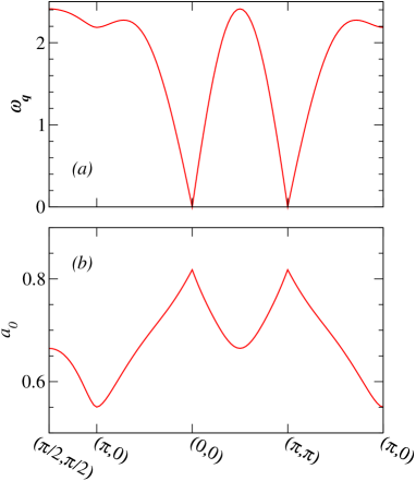
Figure 19: Dispersion relation (a) and wavevector dependence of the relative weight of the magnon pole (b) calculated with the effective Hamiltonian with the parameters $c^{m}=3.1,c^{s}=3.1,\Delta=1.94,g=1.86$, and the spinon-spinon potential $V(r)=-6.2{\rm e}^{-r/2}$.

The ${\bf q}$ dependence of the total spectral weight of the spin system cannot be modeled with our approach here, because the effective model completely neglects the structure of the ground state, replacing it by trivial vacuum, and the magnon creation operator is also an oversimplification of the spin operator. Because of these simplifications the total spectral weight is unity for all ${\bf q}$. A main focus in Secs. III and IV was on the relative weight $a_{0}({\bf q})$ of the leading magnon pole, and this quantity does have its counterpart in Eq. (32);

$$a_{0}({\bf q})=|\langle n=0|d^{\dagger}_{\bf q}|{\rm vac}\rangle|^{2}=|\langle 0|{\bf q}\rangle|^{2},$$ (33)

where $|n=0\rangle\rangle$ is the lowest-energy eigenstate and $a_{0}({\bf q})$ can be compared with the QMC/SAC results in Fig. 10. Given that the Hilbert space of the effective model contains only a single magnon, the spectral function should correspond to the transverse component in situations where the transverse and longitudinal contributions are separated (e.g., polarized neutron scattering).

We now include attractive spinon-spinon interactions such that bare (before mixing with the magnon) bound states are produced, as in Fig. 18. The other model parameters are again adjusted such that the dispersion relation resembles that in the Heisenberg model, with the anomaly at ${\bf q}=(\pi,0)$. The resulting dispersion (location of the dominant $\delta$-function, which constitutes the lower edge of the spectral function) as well as the relative magnon amplitude are graphed in Fig. 19. The dispersion relation is very similar to that obtained without spinon-spinon interactions in Fig. 16. Comparing the amplitude $a_{0}({\bf q})$ in Fig. 19(b) with the Heisenberg results in Fig. 10, we can see very similar features, with minima and maxima at the same wavevectors, though the variations in the amplitude are larger in the Heisenberg model.

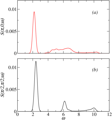
Figure 20: Spectral functions of the effective model at (a) ${\bf q}=(\pi,0)$ and (b) ${\bf q}=(\pi/2,\pi/2)$, using model parameters corresponding to the Heisenberg model; $c^{m}=3.1,c^{s}=3.1,\Delta=1.94,g=1.86$ and the spinon-spinon potential $V(r)=-6.2{\rm e}^{-r/2}$ (same as used in Fig. 18 and 19). The $\delta$-functions in the exact spectral function (computed here using an $L=64$ lattice) have been broadened for visualization.

The full spectral functions at ${\bf q}=(\pi,0)$ and $(\pi/2,\pi/2)$ are displayed in Fig. 20. Here we have broadened all $\delta$-functions to obtain continuous spectral functions. As already discussed, the prominent $\delta$-function corresponding to the magnon is similar to what is observed in the Heisenberg model, though clearly the shapes of the continua above the main $\delta$-function are different from those in Fig. 6. Upon reducing the spinon energy offset $\Delta$ so that the bare energy falls below the magnon energy close to ${\bf q}=(\pi,0)$, we observe a very interesting behavior in Fig. 21. We see that the main magnon peak is washed out, due to decay into the lower spinon states. This is very similar to what we found for the $J$-$Q$ model in Sec. IV, where already a relatively small value of $Q/J$ led to a broad spectrum without magnon pole at ${\bf q}=(\pi,0)$. At $(\pi/2,\pi/2)$ the magnon pole remained strong, however, and this is also what we see for the effective model in Fig. 21. Without spinon-spinon interactions, when the bare magnon is inside the spinon continuum a sharp (single $\delta$-function) spinon-magnon resonance remains in inside the continuum of free spinon states. Thus, for the magnon pole to completely decay, spinon-spinon interactions are essential in the effective model.

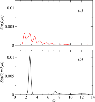
Figure 21: Spectral functions as in Fig. 20, but with the parameters of the effective model chosen to give behaviors similar to the $J$-$Q$ model with $Q\approx J$; $c^{m}=3.1,c^{s}=6.2,\Delta=0.39,g=1.86$ and the spinon-spinon potential $V(r)=-6.2{\rm e}^{-r/2}$.

These results for a simple effective model provide compelling evidence for the mechanism of magnon-spinon mixing outlined above. The results also suggest that the absence of magnon pole at and close to ${\bf q}=(\pi,0)$ does not necessarily imply complete spinon deconfinement, as we have to include explicitly attractive interactions in the effective model in order to reproduce the behavior in the full spin systems. Weak attractive spinon-spinon interactions have previously been detected explicitly in the $J$-$Q$ model at the deconfined critical point tang13 , and they are also expected based on the field-theory description, where the spinons are never completely deconfined due to their coupling to an emergent gauge field senthil04a . The loss of the magnon pole observed here then signifies that the magnon changes character, from a single spatially well-resolved small resonance particle to a more extended particle (with more spinon characteristics) as a weak $Q$ interaction is turned on, and finally the particle completely disintegrating into a continuum of weakly bound spinon pairs and deconfined spinons.

VI Conclusions

We have investigated the long-standing problem of the excitation anomaly at wavevectors ${\bf q}\approx(\pi,0)$ in the spin-$1/2$ square lattice Heisenberg antiferromagnet, and established its relationship to deconfined quantum criticality by also studying the $J$-$Q$ model. Using an improved stochastic (sampling) method for analytic continuation of QMC correlation functions, we have been able to quantify the evolution of the magnon pole in the dynamic structure factor $S({\bf q},\omega)$ as the AFM order is weakened with increasing ratio $Q/J$, all the way from the Heisenberg limit $(Q=0$) to the deconfined critical point at $Q/J\approx 22$. For the Heisenberg model, our results agree with other numerical approaches (series expansions zheng05 and continuous similarity transformations within the Dyson-Maleev formalism Powalski15 ) and also with recent inelastic neutron scattering experiments of the quasi-2D antiferromagnet CFTD piazza15 . Upon increasing $Q/J$, we found a rapid loss of single-magnon weight at ${\bf q}\approx(\pi,0)$, but not at ${\bf q}\approx(\pi/2,\pi/2)$, where the magnon pole remains robust even at the critical point. At first sight these behaviors appear surprising, but we can consistently explain them through the proposed connection to deconfined quantum criticality.

Motivated by the numerical results, we have constructed an effective model of magnon-spinon mixing that can phenomenologically explain not only the fragile, almost fractionalized $(\pi,0)$ magnon of the Heisenberg model and its decay into spinon pairs with increasing $Q/J$, but also establishes the reason of the stability of the $(\pi/2,\pi/2)$ magnon in the $J$-$Q$ model for large $Q$ (as discovered with the QMC-SAC calculations). The essential ingredient is a gapped spinon band with a dispersion minimum at $(\pi,0)$, for which we find motivation in the fact that this point becomes gapless at the deconfined quantum critical point. If the continuum of bare spinon excitations remains above the magnon band throughout the BZ (as in Fig. 16), then the lowest excitations are always magnons. However, since the two bands are coupled in the effective model, via a term that destroys a magnon and creates two spinons (as well as its conjugate destroying the spinons and creating a magnon), the magnons fluctuate in and out of the spinon space, and this effect is the largest at the point in the BZ where the gap between the two bare branches is the smallest, i.e., at ${\bf q}=(\pi,0)$. We find that this effect can account quantitatively for the dip in the magnon dispersion relation, and qualitatively the wavevector dependence of the relative weight of the $\delta$-function at the lower edge of the spectrum is also captured.

Within this effective model, the deconfinement mechanism in the $J$-$Q$ model is explained as the bare spinon dispersion dipping below the magnon at ${\bf q}=(\pi,0)$. This can happen already for small $Q/J$, far away from the AFM–VBS transition, because the bare magnon-spinon gap is already small for $Q=0$. As $Q/J$ increases, an increasing fraction of the BZ becomes deconfined, until finally the gapless spinons deconfine at the critical point. Our QMC-SAC results indicate that the excitations at higher energy remain confined, as exemplified by ${\bf q}=(\pi/2,\pi/2)$. Within the effective model this follows from the bare spinon dispersion staying above the magnon band in this region of wavevectors.

Clearly the effective model should not be taken as a quantitative description of the Heisenberg and $J$-$Q$ systems; motivated by aspects of deconfined quantum-criticality and the AF* state, we have introduced it mainly as a phenomenological tool for elucidating the behaviors observed in the QMC studies of the model Hamiltonians. Nevertheless, it is remarkable how well the essential observed features are captured and how otherwise non-intuitive aspects of the deconfinement mechanism follow naturally from the magnon-spinon mixing under mild assumptions on the bare parameters of the effective model. Thus, even in the absence of a strict microscopic derivation, the effective model can be justified by its many non-trivial confirmed predictions.

Considering the mechanism leading to the loss of magnon pole with increasing $Q$, it is interesting to note that it does not appear to involve significant broadening of the $\delta$-function, but instead the spectral weight of this peak is distributed out into the continuum by the spinon mixing process. This is in accord with the general belief that quantum antiferromagnets with collinear order lack the damping processes that cause the broadening of the magnon pole in frustrated, non-collinear magnets chernyshev06 ; ma16 ; kamiya17 . Our proposed mechanism of spinon mixing is, thus, very different from standard magnon damping.

The scenario of a nearly fractionalized magnon in the Heisenberg model does not necessarily stand in conflict with the expansion in multi-magnon processes Powalski15 ; Powalski17 , which can account for the dynamic structure factor without invoking any spinon mixing effects. We have only discussed the effective model of the excitations at the level of a single magnon and its mixing with the spinon continuum, and our results for the Heisenberg model show that the magnon is significantly dressed by spinons around ${\bf q}=(\pi,0)$ but is not yet fractionalized. The magnon-spinon mixing then represents a description of the internal structure of the magnon, and we have not considered the further effects of multi-magnon processes. It is remarkable that the results of Ref. Powalski17, match the experimental data (and also numerical data for the Heisenberg model) so well without taking into account the internal spinon structure of the magnons, if indeed this structure is present. Here we can draw a loose analogy with nuclear physics, where the inter-nucleon force has an effective description in terms of exchange of mesons (pions) between nucleons. Yukawa proposed mesons as the carriers of the force without knowledge of the quark structure of the nucleons and mesons that is ultimately involved in the interaction (residual strong force) process, and quantitatively satisfactory results in nuclear physics are obtained with the effective interaction (and calculations with the full strong force between quars mediated by gluons are in practice too complicated to work with quantitatively). The significant attractive interaction between magnons in the Heisenberg model Powalski15 ; Powalski17 might perhaps similarily be regarded as mediated by spinon pairs (which themselves constitute magnons), and, by the pion analogy, the magnons and their residual attractive interactions could also provide an accurate description of the excitations without invocing the internal spinon structure. To investigate the relationship between the two pictures further, it would be interesting to treat the $J$-$Q$ model with the method of Ref. Powalski17, . Based on our scenario we predict that the multi-magnon expansion should break down rapidly close to ${\bf q}=(\pi,0)$as the $Q$ interaction is turned on but remain convergent at low energies until the system comes close to the deconfined quantum-critical point.

The fragility of the magnons at and close to ${\bf q}=(\pi,0)$ suggests that these excitations may become completely fractionalized also by other interactions than the $Q$-terms considered here, e.g., ring exchange or longer-range pair exchange. These interactions have recently also been investigated in the context of possible topological order and spinon excitations in the cuprates chatterjee17 . Earlier the so-called AF* state had been proposed, largely on phenomenological grounds, where topological order coexists with AFM order and there is a spinon continuum similar to the one in our effective model balents99 ; senthil00 . Though in our scenario the reason for the spinon continuum is different—the proximity to a deconfined quantum critical point—a generic conclusion valid in either case is that spinon deconfinement can set in at ${\bf q}=(\pi,0)$ well before any ground state transition at which the low-energy spinons deconfine.

In this context the quasi-2D square-lattice antiferromagnet Cu(pz)₂(ClO₄)₂ is very interesting. It has a weak frustrated next-nearest-neighbor coupling and has been modeled within the $J_{1}$-$J_{2}$ Heisenberg model tsyrulin09 . Neutron scattering experiments on the material and series-expansion calculations for the model show an even larger suppression of the $(\pi,0)$ energy than in the pure Heisenberg model, similar to what we have observed in the presence of a weak $Q$ interaction. The experimental $(\pi,0)$ line shape also seems to have a smaller magnon pole than CFTD, in accord with our scenario of a fragile magnon pole, although we are not aware of any quantitative analysis of the weight of the magnon pole and no line-shape calculations were reported in Ref. tsyrulin09, . It would clearly be intersting to carry out neutron experiments at higher resolution and to make detailed comparisons with calculations beyond the dispersion relation.

Ultimately the $J_{1}$-$J_{2}$ system should be different from the $J$-$Q$ model, because the deconfined quantum critical point of the latter most likely is replaced by an extended gapless spin liquid phase of the former hu13 ; gong14 ; morita15 ; wang17 . However, since this phase should also be associated with deconfined spinons, the evolution of the excitations as this phase is approached may be very similar to what we have discussed within the $J$-$Q$ model on its approach to the deconfined quantum critical point. A state with topological order and spinon excitations may instead be approached when strong ring-exchange interactions are added chatterjee17 , but given that $J$ is weak in Cu(pz)₂(ClO₄)₂ these interactions may not play a significant role in this case. Ring exchange should be more important in Sr₂CuO₂Cl₂, where excitation anomalies have also been observed guarise10 .

The magnetic-field ($h$) dependence of the excitation spectrum of Cu(pz)₂(ClO₄)₂ was also studied in Ref. tsyrulin09, . Since the energy scale of the Heisenberg exchange is even smaller than in CFTD, it was possible to study field strengths of order $J$ and observe significant changes in the dispersion relation and the $(\pi,0)$ line shape. The methods we have developed here can also be applied to systems in an external magnetic field and it would be interesting to study the dynamics of the $J$-$Q$-$h$ model. Some results indicating destabilization of magnons due to the field in the Heisenberg model are already available syljuasen08b , and our improved analytic continuation technique could potentially improve on the frequency resolution.

Appendix A Covariance in QMC and synthetic data

As discussed in Sec. II.1 the QMC-computed imaginary time data $\bar{G}(\tau_{i})$ for different $i$ are correlated, and it is well known jarrell96 that this has to be taken into account in any statistically proper analytic continuation procedure (though in practice good results can still be obtained with just the diagonal elements $\sigma_{i}$, if they are sufficiently small). While the covariance may seem like a nuisance, there is actually a silver lining, in that correlations between different $\tau$-points typically imply that the data are actually better than the individual statistical errors $\sigma_{i}$ might indicate.

As an extreme example of the above, imagine a situation in which all data points are perfectly correlated in the sense that the computed $\bar{G}_{i}$ (over a bin or the whole simulation) is of the form

$$G_{i}=G^{\rm exact}_{i}(1+\sigma)$$ (34)

for all $i$, where $\sigma$ is the common noise source. Then, upon normalization, $G_{i}\to G_{i}/G_{0}$, one obtains the exact value $G^{\rm exact}_{i}/G^{\rm exact}_{0}$ (where the subscript $0$ corresponds to $\tau=0$). In reality the noises for different $\tau$-points are not perfectly correlated, but have an autocorrelation function that decays with $\tau$, but nevertheless the presence of covariance corresponds to additional information content in the data set, and this information can improve the frequency resolution when compared to the case of no off-diagonal elements of $C$ and the same values of all $\sigma_{i}=C_{ii}$. Here we show some examples of covariance-effects in QMC data, and also explain how we build in correlated noise in synthetic data.

A.1 Real QMC data

In Fig. 22 we show an example of data underlying the SAC calculations in Sec. III; at the most interesting wavevector, ${\bf q}=(\pi,0)$, for a system with $L=48$. We have here used a quadratic $\tau$-grid, in order to take advantage of the reduced error bars close to $\tau=0$ after normalizing to $G(0)=1$, while not including an excessively large number of points (in which case there is a lot of redundancy in the correlated data and it also becomes difficult to diagonalize the covariance matrix). We only include data points for which the relative errors $\sigma_{i}/\bar{G}_{i}$ are less than $10\%$.

Fig. 22(a) shows the $G(\tau)$ data on a lin-log scale, so that a pure exponential decay (arising from a spectrum with a single $\delta$-function) corresponds to a straight line. From the analysis in Sec. III we have that the amplitude of the magnon $\delta$-function is $a_{0}=0.405\pm 0.025$ and its frequency is $\omega_{0}\approx 2.13$. The two straight lines in the figure correspond to the contribution from this $\delta$-function when the amplitude is the mean value plus or minus one error bar, i.e., $0.38$ and $0.43$, respectively. These lines are still significantly below the data points and it is also clear that the data have not quite converged to a pure straight line at the largest $\tau$ available. Therefore, it is not easy to extract $a_{0}$ and $\omega_{0}$ from a simple exponential fit to the large-$\tau$ data, and the SAC procedure with the special treatment of the magnon pole should be an optimal way to take into account the effects of the continuum.

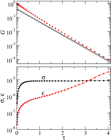
Figure 22: (a) Imaginary-time correlation function at $q=(\pi,0)$ for 2D Heisenberg lattice with $L=48$, computed in SSE QMC simulations at $\beta=192$ (giving $T=0$ results for all practical purposes). The two straight lines correspond to the contribution for the leading $\delta$-function obtained in the SAC procedure, with amplitude $a_{0}=0.405\pm 0.025$. (b) The statistical errors (diagonal elements of the covariance matrix) $\sigma(\tau)$ and the eigenvalues of the covariance matrix (ordered from smallest to largest).

It is also interesting to examine the eigenvectors of the covariance, i.e., the linear combinations,

$${\bf v_{n}}=\sum_{i}v_{n}(i)G(\tau_{i}),$$ (35)

of the imaginary-time data points that fluctuate independently of each other in the QMC simulations. Figure 23 shows three of the normalized eigenvectors corresponding to the eigenvalues in Fig. 22. Note that the normalization of $G(\tau_{i})$ has already removed a significant component of the covariance—the uniformly fluctuating component—and without the normalization the largest eigenvector has the most weight for small $\tau_{i}$, instead of being shifted to higher $\tau_{i}$ with the normalized data set (seen for $n=1$ in the figure). The vector corresponding to smallest eigenvalue has alternating positive and negative values and decays rapidly with $\tau_{i}$.

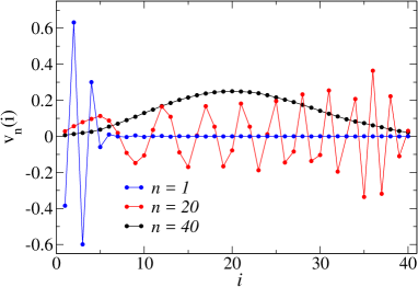
Figure 23: The eigenvectors corresponding to the smallest ($n=1$) and largest ($n=40$) eigenvalues of the covariance matrix in Fig. 22, as well as one from the middle of the eigenvalue spectrum ($n=20$).

A.2 Synthetic data

In order to be able to test all aspects of the SAC procedures used with real QMC data, we generate a number $N_{B}$ of bins of noisy data starting from the exact $G(\tau)$ computed from Eq. (4) with the given synthetic spectrum $S(\omega)$. These bins are used to compute the mean values $\bar{G}_{i}$ and the covariance matrix with the same program used to process the QMC data. To construct correlated noise similar to that present in QMC data, for each bin we first generate a set of normal-distributed random numbers $\sigma^{0}_{i}$, with a given standard deviation (the same for all $i$, which is not necessarily exactly the case with QMC data but should be good enough for testing purposes). We then run these data through a correlation procedure where a new noise set is generated according to

$$\sigma_{i}=\frac{\sum_{j}\sigma^{0}_{j}{\rm e}^{-|\tau_{i}-\tau_{j}|/\xi_{\tau}}}{\sqrt{\sum_{j}{\rm e}^{-2|\tau_{i}-\tau_{j}|/\xi_{\tau}}}}$$ (36)

with a given autocorrelation time $\xi_{\tau}$. These noise values are then added to $G_{i}$. The autocorrelation time and the original noise level $\sigma^{0}_{i}$ can be adjusted so that the eigenvalues of the covariance matrix are similar to those of typical QMC data, though the QMC correlations can of course not be expected to exactly follow what is produced by Eq. (36). An example is shown in Fig. 24, where we have adjusted the parameters of Eq. (36) to match the real QMC data in Fig. 22 closely (apart from an overall factor $\approx 2$ in the $\tau$-scale). As is apparent, we can indeed obtain very similar forms of the standard errors and the eigenvalues of the covariance matrix.

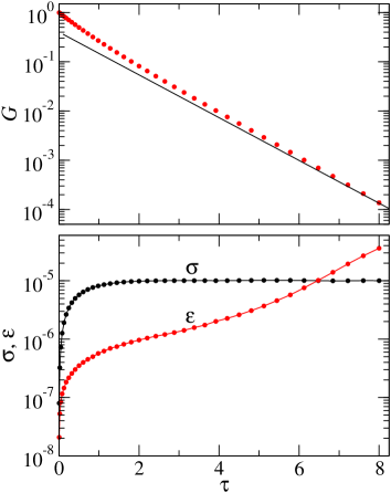
Figure 24: The same kind of data as in Fig. 22 but obtained using a synthetic spectrum with a $\delta$-function of weight $a_{0}=0.4$ at $\omega_{0}=1$ and a continuum consisting of a half-Gaussian above the $\delta$-function, of width $1$. The straight line in (a) corresponds to the contribution from just the $\delta$-function.

References

- (1) P. W. Anderson, An Approximate Quantum Theory of the Antiferromagnetic Ground State, Phys. Rev. 86, 694 (1952).
- (2) P. W. Anderson, The resonating valence bond state in \chemfigLa_2CuO_4 and superconductivity, Science 235, 1196 (1987).
- (3) E. Manousakis, The spin-1/2 Heisenberg antiferromagnet on a square lattice and its application to the cuprous oxides, Rev. Mod. Phys. 63,1 (1991).
- (4) E. J. Neves and J. F. Peres, Long range order in the ground state of two-dimensional antiferromagnets, Phys. Lett. A 114, 331 (1986).
- (5) R. R. P. Singh, Thermodynamic parameters of the T=0, spin-1/2 square-lattice Heisenberg antiferromagnet, Phys. Rev. B 39, R9760 (1989).
- (6) J. D. Reger and A. P. Young, Monte Carlo simulations of the spin- Heisenberg antiferromagnet on a square lattice, Phys. Rev. B 37, 5978 (1988).
- (7) K. J. Runge, Quantum Monte Carlo calculation of the long-range order in the Heisenberg antiferromagnet, Phys. Rev. B 45, 7229 (1992).
- (8) A. W. Sandvik, Finite-size scaling of the ground-state parameters of the two-dimensional Heisenberg model, Phys. Rev. B 56, 11678 (1997).
- (9) A. W. Sandvik and H. G. Evertz, Loop updates for variational and projector quantum Monte Carlo simulations in the valence-bond basis, Phys. Rev. B 82, 024407 (2010).
- (10) F.-J. Jiang and U.-J. Wiese, High-precision determination of low-energy effective parameters for a two-dimensional Heisenberg quantum antiferromagnet, Phys. Rev. B 83, 155120 (2011).
- (11) B. B. Beard and U.-J. Wiese, Simulations of Discrete Quantum Systems in Continuous Euclidean Time, Phys. Rev. Lett. 77, 5130 (1996).
- (12) J.-K. Kim and M. Troyer, Low Temperature Behavior and Crossovers of the Square Lattice Quantum Heisenberg Antiferromagnet, Phys. Rev. Lett. 80, 2705 (1998).
- (13) B. B. Beard, R. J. Birgeneau, M. Greven, and U.-J. Wiese, Square-Lattice Heisenberg Antiferromagnet at Very Large Correlation Lengths, Phys. Rev. Lett. 80, 1742 (1998).
- (14) S. Chakravarty, B. I. Halperin, and D. R. Nelson, Two-dimensional quantum Heisenberg antiferromagnet at low temperatures, Phys. Rev. B 39, 2344 (1989).
- (15) P. Hasenfratz and F. Niedermayer, Finite size and temperature effects in the AF Heisenberg model, Z. Phys. B 92, 91 (1993).
- (16) R. R. P. Singh and M. P. Gelfand, Spin-wave excitation spectra and spectral weights in square lattice antiferromagnets, Phys. Rev. B 52, R15695 (1995).
- (17) A. W. Sandvik and R. R. P. Singh, High-energy magnon dispersion and multimagnon continuum in the two-dimensional Heisenberg antiferromagnet, Phys. Rev. Lett. 86, 528 (2001).
- (18) M. Powalski, G. S. Uhrig, and K. P. Schmidt, Roton Minimum as a Fingerprint of Magnon-Higgs Scattering in Ordered Quantum Antiferromagnets, Phys. Rev. Lett. 115, 207202 (2015).
- (19) M. Powalski, K. P. Schmidt, and G. S. Uhrig, Mutually attracting spin waves in the square-lattice quantum antiferromagnet, arXiv:1701.04730.
- (20) W. Zheng, J. Oitmaa, and C. J. Hamer, Series studies of the spin-1/2 Heisenberg antiferromagnet at T =0: Magnon dispersion and structure factors, Phys. Rev. B 71, 184440 (2005).
- (21) J. Igarashi, 1/S expansion for thermodynamic quantities in a two-dimensional Heisenberg antiferromagnet at zero temperature, Phys. Rev. B 46, 10763 (1992).
- (22) C. M. Canali and M. Wallin, Spin-spin correlation functions for the square-lattice Heisenberg antiferromagnet at zero temperature, Phys. Rev. B 48, 3264 (1993).
- (23) J. Igarashi and T. Nagao, -expansion study of spin waves in a two-dimensional Heisenberg antiferromagnet, Phys. Rev. B 72, 014403 (2005).
- (24) A. V. J. Syromyatnikov, Spectrum of short-wavelength magnons in a two-dimensional quantum Heisenberg antiferromagnet on a square lattice: Third-order expansion in 1/S, J. Phys. Condens. Matter 22, 216003 (2010).
- (25) R. Coldea, S. M. Hayden, G. Aeppli, T. G. Perring, C. D. Frost, T. E. Mason, S.-W. Cheong, and Z. Fisk, Spin waves and electronic interactions in \chemfigLa_2CuO_4, Phys. Rev. Lett. 86, 5377 (2001).
- (26) N. S. Headings, S. M. Hayden, R. Coldea, and T. G. Perring, Anomalous high-energy spin excitations in the high-Tc superconductor-parent antiferromagnet \chemfigLa_2CuO_4, Phys. Rev. Lett. 105, 247001 (2010).
- (27) N. M. R. Peres and M. A. N. Araújo, Spin-wave dispersion in \chemfigLa_2CuO_4, Phys. Rev. B 65, 132404 (2002).
- (28) X. Wan, T. A. Maier, and S. Y. Savrasov, Calculated magnetic exchange interactions in high-temperature superconductors, Phys. Rev. B 79, 155114 (2009).
- (29) J.-Y. P. Delannoy, M. J. P. Gingras, P. C. W. Holdsworth, and A.-M. S. Tremblay, Low-energy theory of the --- Hubbard model at half-filling: Interaction strengths in cuprate superconductors and an effective spin-only description of \chemfigLa_2CuO_4, Phys. Rev. B 79, 235130 (2009).
- (30) B. D. Piazza, M. Mourigal, M. Guarise, H. Berger, T. Schmitt, K. J. Zhou, M. Grioni, and H. M. Rønnow, Unified one-band Hubbard model for magnetic and electronic spectra of the parent compounds of cuprate superconductors, Phys. Rev. B 85, 100508(R) (2012).
- (31) H. M. Rønnow, D. F. McMorrow, R. Coldea, A. Harrison, I. D. Youngson, T. G. Perring, G. Aeppli, O. Syljuåsen, K. Lefmann, and C. Rischel, Spin dynamics of the 2D spin-1/2 quantum antiferromagnet copper deuteroformate tetradeuterate (CFTD), Phys. Rev. Lett. 87, 037202 (2001).
- (32) N. B. Christensen, H. M. Rønnow, D. F. McMorrow, A. Harrison, T. G. Perring, M. Enderle, R. Coldea, L. P. Regnault, and G. Aeppli, Quantum dynamics and entanglement of spins on a square lattice, Proc. Natl Acad. Sci. USA 104, 15264(2007).
- (33) B. Dalla Piazza, M. Mourigal, N. B. Christensen, G. J. Nilsen, P. Tregenna-Piggott, T. G. Perring, M. Enderle, D. F. McMorrow, D. A. Ivanov, and H. M. Rønnow, Fractional excitations in the square-lattice quantum antiferromagnet, Nat.Phys. 11, 62 (2015).
- (34) Y. Tang and A. W. Sandvik, Confinement and deconfinement of spinons in two dimensions, Phys. Rev. Lett. 110, 217213 (2013).
- (35) The weight of the magnon pole was not reported in Ref. Powalski17 , but the authors have confirmed to us that the calculations do give weights similar to those in Refs. Singh95 and sandvik01 .
- (36) A. W. Sandvik, Evidence for Deconfined Quantum Criticality in a Two-Dimensional Heisenberg Model with Four-Spin Interactions, Phys. Rev. Lett. 98, 227202 (2007).
- (37) R. G. Melko and R. K. Kaul, Scaling in the Fan of an Unconventional Quantum Critical Point, Phys. Rev. Lett. 100, 017203 (2008).
- (38) K. Harada, T. Suzuki, T. Okubo, H. Matsuo, J. Lou, H. Watanabe, S. Todo, and N. Kawashima, Possibility of deconfined criticality in SU(N) Heisenberg models at small N, Phys. Rev. B 88, 220408 (2013).
- (39) H. Shao, W. Guo, and A. W. Sandvik, Quantum criticality with two length scales, Science 352, 213 (2016).
- (40) T. Senthil, A. Vishwanath, L. Balents, S. Sachdev, and M. P. A. Fisher, Deconfined quantum critical points, Science 303, 1490 (2004).
- (41) T. Senthil, A. Vishwanath, L. Balents, S. Sachdev, and M. P. A. Fisher, Quantum criticality beyond the Landau-Ginzburg-Wilson paradigm, Phys. Rev. B 70, 144407 (2004).
- (42) L. Spanu, F. Becca, and S. Sorella, Theoretical constraints for the magnetic-dimer transition in two-dimensional spin models, Phys. Rev. B 73, 134429 (2006).
- (43) H. Suwa, A. Sen and A. W. Sandvik, Level spectroscopy in a two-dimensional quantum magnet: Linearly dispersing spinons at the deconfined quantum critical point, Phys. Rev. B 94, 144416 (2016).
- (44) L. Balents, M. P. A. Fisher, and C. Nayak, Dual order parameter for the nodal liquid, Phys. Rev. B 60, 1654 (1999).
- (45) T. Senthil and M. P. A. Fisher, Z2 Gauge Theory of Electron Fractionalization in Strongly Correlated Systems, Phys. Rev. B 62, 7850 (2000).
- (46) H. Shao and A. W. Sandvik, unpublished.
- (47) A. W. Sandvik, Computational Studies of Quantum Spin Systems, AIP Conf. Proc. 1297, 135 (2010).
- (48) A. W. Sandvik, A generalization of Handscomb’s quantum Monte Carlo scheme—Application to the 1-D Hubbard model, J. Phys. A 25, 3667 (1992).
- (49) A. W. Sandvik, R. R. P. Singh, and D. K. Campbell, Quantum Monte Carlo in the interaction representation—Application to a spin-Peierls model, Phys. Rev. B 56, 14510 (1997).
- (50) H.-B. Schüttler and D. J. Scalapino, Monte Carlo studies of the dynamical response of quantum many-body systems, Phys. Rev. B 34, 4744 (1986).
- (51) A. W. Sandvik, Stochastic method for analytic continuation of quantum Monte Carlo data, Phys. Rev. B 57, 10287 (1998).
- (52) S. F. Gull and J. Skilling, Maximum entropy method in image processing, Proc. IEEE 131, 646 (1984).
- (53) R. N. Silver, D. S. Sivia, and J. E. Gubernatis, Maximum-entropy method for analytic continuation of quantum Monte Carlo data, Phys. Rev. B 41, 2380 (1990); J. E. Gubernatis, M. Jarrell, R. N. Silver, and D. S. Sivia, Quantum Monte Carlo simulations and maximum entropy: Dynamics from imaginary-time data, ibid. 44, 6011 (1991).
- (54) M. Jarrell and J. E. Gubernatis, Bayesian inference and the analytic continuation of imaginary-time quantum Monte Carlo data, Phys. Rep. 269, 133 (1996).
- (55) K. S. D. Beach, Identifying the maximum entropy method as a special limit of stochastic analytic continuation, arXiv:cond-mat/0403055.
- (56) O. F. Syljuåsen, Using the average spectrum method to extract dynamics from quantum Monte Carlo simulations, Phys. Rev. B 78, 174429 (2008).
- (57) S. Fuchs, T. Pruschke, and M. Jarrell, Analytic continuation of quantum Monte Carlo data by stochastic analytical inference, Phys. Rev. E 81, 056701 (2010).
- (58) A. S. Mishchenko, N. Nagaosa, N. V. Prokof’ev, A. Sakamoto, and B. V. Svistunov, Self-trapping of polarons in the Rashba-Pekar model, Phys. Rev. B 66, 020301(R) (2002).
- (59) A. W. Sandvik, Constrained sampling method for analytic continuation, Phys. Rev. E 94, 063308 (2016).
- (60) Y. Q. Qin, B. Normand, A. W. Sandvik, and Z. Y. Meng, Amplitude mode in three-dimensional dimerized antiferromagnets, Phys. Rev. Lett. 118, 147207 (2017).
- (61) In principle the cross-section also involves a form factor, corresponding to the finite extent of the orbitals hosting the localized spins, but in most cases of interest the momentum-dependence of the form factor is very weak and can be neglected.
- (62) A. L. Chernyshev and M. E. Zhitomirsky, Magnon Decay in Noncollinear Quantum Antiferromagnets, Phys. Rev. Lett. 97, 207202 (2006).
- (63) A. L. Chernyshev and M. E. Zhitomirsky, Spin waves in a triangular lattice antiferromagnet: Decays, spectrum renormalization, and singularities, Phys. Rev. B 79, 144416 (2009).
- (64) A. Sen, H. Suwa and A. W. Sandvik, Velocity of excitations in ordered, disordered and critical antiferromagnets, Phys. Rev. B 92, 195145 (2015).
- (65) E. Dagotto and A. Moreo, Phase diagram of the frustrated spin-1/2 Heisenberg antiferromagnet in 2 dimensions, Phys. Rev. Lett. 63, 2148 (1989).
- (66) M. P. Gelfand, R. R. P. Singh, and D. Huse, Zero-temperature ordering in two-dimensional frustrated quantum Heisenberg antiferromagnets, Phys. Rev. B 40, 10801 (1989).
- (67) W.-J. Hu, F. Becca, A. Parola, and S. Sorella, Direct evidence for a gapless Z2 spin liquid by frustrating Néel antiferromagnetism, Phys. Rev. B 88, 060402(R) (2013).
- (68) S.-S. Gong, W. Zhu, D. N. Sheng, O. I. Motrunich, and M. P. A. Fisher, Plaquette Ordered Phase and Quantum Phase Diagram in the Spin- - Square Heisenberg Model, Phys. Rev. Lett. 113, 027201 (2014).
- (69) S. Morita, R. Kaneko, and M. Imada, Quantum Spin Liquid in Spin- - Heisenberg Model on Square Lattice: Many-Variable Variational Monte Carlo Study Combined with Quantum-Number Projections, J. Phys. Soc. Jpn. 84, 024720 (2015).
- (70) L. Wang and A. W. Sandvik, Critical level crossings and gapless spin liquid in the square-lattice spin- - Heisenberg antiferromagnet, arXiv:1702.08197.
- (71) J. J. Hopfield, Theory of the Contribution of Excitons to the Complex Dielectric Constant of Crystals, Phys. Rev. 112, 1555 (1958).
- (72) G. D. Mahan, Many-Particle Physics, third edition (Plenum 2000).
- (73) G. Möller, H. Thomas, H. Beck, and J. C. Bonner, Quantum spin dynamics of the antiferromagnetic linear chain in zero and nonzero magnetic field, Phys. Rev. B 24, 1429 (1981).
- (74) L. D. Faddeev and L. A. Takhtajan, What is the spin of a spin wave?, Phys. Lett. A 85, 375 (1981).
- (75) J. Ma, Y. Kamiya, T. Hong, H. B. Cao, G. Ehlers, W. Tian, C. D. Batista, Z. L. Dun, H. D. Zhou, and M. Matsuda, Static and Dynamical Properties of the Spin-1/2 Equilateral Triangular-Lattice Antiferromagnet Ba3CoSb2O9, Phys. Rev. Lett. 116, 087201 (2016).
- (76) Y. Kamiya, L. Ge, T. Hong, Y. Qiu, D. L. Quintero-Castro, H. B. Cao, M. Matsuda, C. D. Batista, M. Mourigal, H. D. Zhou, and J. Ma, Role of Quantum Fluctuations in Ba3CoSb2O9 Revealed by Excitations within the 1/3-Magnetization Plateau, arXiv:1701.07971.
- (77) S. Chatterjee, S. Sachdev, and M. S. Scheurer, Intertwining topological order and broken symmetry in a theory of fluctuating spin density waves, arXiv:1705.06289.
- (78) N. Tsyrulin, T. Pardini, R. R. P. Singh, F. Xiao, P. Link, A. Schneidewind, A. Hiess, C. P. Landee, M. M. Turnbull, and M. Kenzelmann, Quantum Effects in a Weakly Frustrated Two-Dimensional Heisenberg Antiferromagnet in an Applied Magnetic Field, Phys. Rev. Lett. 102, 197201 (2009).
- (79) M. Guarise et al., Measurement of Magnetic Excitations in the Two-Dimensional Antiferromagnetic Sr2CuO2Cl2 Insulator Using Resonant X-Ray Scattering: Evidence for Extended Interactions, Phys. Rev. Let. 105, 157006 (2010).
- (80) O. F. Syljuåsen, Numerical evidence for unstable magnons at high fields in the Heisenberg antiferromagnet on the square lattice, Phys. Rev. B 78, 180413(R) (2008).