Andreev-Bashkin effect in superfluid cold gases mixtures

Abstract

We study a mixture of two superfluids with density-density and current-current (Andreev-Bashkin) interspecies interactions. The Andreev-Bashkin coupling gives rise to a dissipationless drag (or entrainment) between the two superfluids. Within the quantum hydrodynamics approximation, we study the relations between speeds of sound, susceptibilities and static structure factors, in a generic model in which the density and spin dynamics decouple. Due to translational invariance, the density channel does not feel the drag. The spin channel, instead, does not satisfy the usual Bijl-Feynman relation, since the f-sum rule is not exhausted by the spin phonons. The very same effect on one dimensional Bose mixtures and their Luttinger liquid description is analysed within perturbation theory. Using diffusion quantum Monte Carlo simulations of a system of dipolar gases in a double layer configuration, we confirm the general results. Given the recent advances in measuring the counterflow instability, we also study the effect of the entrainment on the dynamical stability of a superfluid mixture with non-zero relative velocity.

I Introduction

Mixtures of different kinds of miscible superfluids arise in various areas of physics, starting from the first experiments on ³He-⁴He mixtures Edwards et al. (1965), through possible applications to astrophysical objects Alpar et al. (1984); Kobyakov and Pethick (2017), all the way to the more recent developments in the fields of superconductivity Garaud et al. (2014), cold atoms Modugno et al. (2002); Catani et al. (2008); Roy et al. (2017) and exciton-polariton condensates Lagoudakis et al. (2009).

The statistics of each component of the mixture can be arbitrary, and Bose-Bose, Bose-Fermi, and Fermi-Fermi mixtures were all successfully realised experimentally in cold gases. In these experiments, also the chemical nature of the components can vary: the use of two different elements, of different isotopes of the same element, and of different internal states of a common isotope were demonstrated. The ability to reach simultaneous quantum degeneracy in such a wide variety of atomic species in cold gases experiments allows for the realisation of very diverse interactions between the two component superfluids.

One of the most elusive effect of coupled superfluids is the existence of a non-zero entrainment between them. The presence of mutual transport has been pointed out for the first time in the 1970s by Andreev and Bashkin Andreev and Bashkin (1976), correcting some previous work on three-fluid hydrodynamics Khalatnikov (1957); Mineev (1975). The most prominent feature of such an effect, nowadays known as Andreev-Bashkin effect (AB), is that the superfluid current $\mathbf{j}_{i}$ of one component will in general depend also on the superfluid velocity ${\bf v}_{j}$ of the other component, or, in other words, that the superfluid density is a non-diagonal matrix, $\rho_{ij}$, namely,

$${\bf j}_{i}=\rho_{ij}{\bf v}_{j},$$ (1)

with the indices $i,j=\{1,2\}$ labelling the species and implicit summation on repeated indices. We shall refer to the off-diagonal element $\rho_{12}$ of the superfluid density matrix as the superfluid drag. Phenomenologically, a nonzero $\rho_{12}$ carries important implication in the dynamics of vortices of a superfluid mixture. Notably, it is predicted that the circulation leading to the stable vortex configurations change abruptly as $\rho_{12}$ is varied, giving rise to stable multiply circulating vortex configurations Meyerovich (1984)

Despite its introduction was inspired by the problem of ³He and ⁴He superfluid mixtures, the low miscibility of these two fluids makes this system hardly achievable in experiments. The AB mechanism has instead recently found applications in the domains of astrophysics and of cold atom systems. In the astrophysical literature, it has been hypothesised that the AB effect could be the source of several peculiar behaviours in neutron stars cores Alpar et al. (1984), which modern models predict to be composed of a mixture of neutrons and protons, both in a superfluid phase (see Lattimer and Prakash (2004); Babaev (2004) and reference therein). Cold atom experiments, on the other hand, thanks to their flexibility and tunability, could open the way to a direct measurement of superfluid drag, albeit this will still require some careful analysis and mitigation of common drawbacks. For instance, calculations within the Bogoliubov theory for Bose-Einstein condensates with typical repulsive interaction—where quantum fluctuations are depressed—predict the AB to be very small Fil and Shevchenko (2004, 2005). Quantum fluctuations can be enhanced by increasing the interactions, but this would also intensify three-body losses, which could be in turn suppressed by confining the system in low dimensional geometries or introducing an optical lattice, as studied, e.g., in Linder and Sudbø (2009); Hofer et al. (2012). However, optical lattices break translational invariance, thus strongly reducing the superfluid density even a $T=0$. We recall that, in continuous space (and with time-reversal symmetry), the superfluid density approaches the total density as $T$ is lowered to zero (see, e.g., Leggett (1998)).

Aside from making the AB mechanism efficient, a very important question is how to measure experimentally its strength. The dynamical protocols typically proposed require the ability to initialise a superfluid current in one component and then observe the onset of dissipationless transport in the other one, initially at rest. For best results, these kind of measurements would likely require a ring geometry and can be of difficult interpretation, since a number of decay processes are present Beattie et al. (2013); Abad et al. (2014).

In the present work, we address some of the above mentioned issues. In particular, we derive some relations between the superfluid drag and other measurable quantities, such as the susceptibilities of the system and the speeds of sound. For systems with $\mathbb{Z}_{2}$ symmetry between the two species, in which spin and density channels decouple, the density channel follows the usual relations, whereas we show how the AB breaks the usual Bijl-Feynman relation for the spin channel. Our findings open the way to measuring the superfluid drag experimentally using standard static and dynamic observables.

To provide support to our theoretical predictions, we study quantitatively a specific model which can show large entrainment, i.e., a dipolar Bose gas trapped in a bilayer configuration. Using the diffusion quantum Monte Carlo method, we extract the dispersion relations, the susceptibilities, the structure factors and the superfluid densities. We show that they satisfy, in a proper regime, the expression derived in the general theory. In particular, it is shown that the standard expression relating the square of the spin speed of sound to the inverse of the susceptibility is inapplicable and it should be corrected by a factor proportional to the superfluid drag. Another possible quantity which could reveal the presence of a superfluid drag is the shift in the position of the dynamical instability. We report a general stability analysis of the mixture, and derive a simple analytical expression for the onset of the dynamical instability to linear order in the drag.

As mentioned above, the AB mechanism could play a more prominent role in low dimensionality. We discuss the modifications to Luttinger liquid theory necessary to describe coupled one dimensional superfluids. We find that, in analogy with the general description, the spin Luttinger parameters, as derived by means of perturbative or ab-initio calculations, receive a correction from the superfluid drag, which could become particularly relevant in the strongly interacting (Tonks-Girardeau) regime.

The paper is organised as follows. In Sec. II we recall the main aspects of the AB effect, which are then analysed within a minimal quantum hydrodynamic toy model in Sec. III. The relations among experimentally relevant observables are derived. The Luttinger liquid theory for one dimensional coupled superfluid is corrected for the presence of AB in the same section. Numerical evidence in support of our theoretical findings are reported in Sec. IV, where we analyse the presence and magnitude of the superfluid drag in a bilayer system of dipolar bosons. In Sec. V we study the dynamical instability of the mixture with respect to the relative velocity between the two fluids. Conclusions and future perspectives are drawn in Sec. VI. For the sake of completeness, the derivations of some relations used in the main text are postponed to the appendices without affecting the comprehension of the main results.

II Andreev-Bashkin effect

Microscopically, the current drag originates from the interactions between two superfluids, leading to the formation of quasi-particles with nonzero content of either of the two species. It is then easy to understand that the transport properties of the two components are not independent: the flow of one component must be accompanied by mass transport of the other component Andreev and Bashkin (1976).

Some important relations concerning the superfluid densities in Eq. (1) can be easily obtained by considering the kinetic energy contribution in the expansion of the ground state energy in terms of the superfluid velocities Kaurov et al. (2005). Due to Galilean invariance, if $\phi_{i}$ is the phase of the superfluid order parameter for component $i$, of mass $m_{i}$, its velocity is given by ${\bf v}_{i}=(\hbar/m_{i})\nabla\phi_{i}$ and the energy due to the superfluid velocities can be written as

$$\delta E=\int d^{D}x\,\sum_{ij}\frac{\hbar^{2}}{2m_{i}m_{j}}\rho_{ij}\nabla\phi_{i}\cdot\nabla\phi_{j}.$$ (2)

By performing a Galilean boost with velocity ${\bf V}$, the phases are shifted to $\phi^{\prime}_{i}=\phi_{i}-(m_{i}/\hbar){\bf V}\cdot{\bf r}$, and the energy change, to first order in ${\bf V}$, is $\delta E^{\prime}=\delta E-\int{\bf P}\cdot{\bf V}\,d^{D}x$, with ${\bf P}/\hbar=\sum_{i}(\rho_{i}+\rho_{12})/m_{i}\nabla\phi_{i}$ the momentum density. Since on the other hand one must have ${\bf P}=n_{1}\nabla\phi_{1}+n_{2}\nabla\phi_{2}$, with $n_{1,2}$ the number densities, the superfluid densities must satisfy

$$m_{i}n_{i}=\rho_{i}+\rho_{12}.$$ (3)

Introducing the effective masses $m_{1,2}^{*}$ through $\rho_{ii}\equiv n_{i}m_{i}^{2}/m_{i}^{*}$, we obtain

$$\rho_{12}=n_{i}m_{i}\left(1-\frac{m_{i}}{m^{*}_{i}}\right),$$ (4)

which provides the relation between the superfluid drag and the effective masses and a constraint for the effective mass ratio.

III Quantum hydrodynamic model

In general, the presence of effective masses changes the relation between static and dynamical properties of the system, and the possibility for some excitation modes to exhaust the sum rules. Let us consider a superfluid mixture with an energy density $e(n_{1},n_{2})$. Expanding the energy around its ground state value to second order in the density fluctuations $\Pi_{i}(x)$ and adding it to Eq. (2) we obtain a hydrodynamic Hamiltonian for two miscible superfluids,

$$H=\frac{1}{2}\sum_{ij}\int\left(\rho_{ij}\frac{\hbar\nabla\phi_{i}}{m_{i}}\cdot\frac{\hbar\nabla\phi_{j}}{m_{j}}+\alpha_{ij}\Pi_{i}\Pi_{j}\right)\,d^{D}x,$$ (5)

where the matrix $\alpha_{ij}=\partial^{2}e/\partial n_{i}\partial n_{j}$ contains the information on inter- and intra-species interactions of the two fluids. Hamiltonian (5) by requiring that the fields $\phi_{i}$ and $\Pi_{j}$ satisfy canonical commutation relations for bosons, i.e., $[\phi_{i}(x),\Pi_{j}(y)]=i\hbar\delta_{ij}\delta(x-y)$.

For the sake of clarity, we take the two superfluids to be equal: $\rho_{ii}=\rho$, $\alpha_{ii}=\alpha$, $m_{i}=m$ and $n_{i}=n/2$, with $n\equiv N/V$ the total number density of the system (see Appendix A for the non-symmetric case). Due to the assumed $\mathbb{Z}_{2}$ symmetry, the dynamics of this model decouples if we rewrite it in terms of the new fields

$$\phi_{d(s)}=(\phi_{1}\pm\phi_{2})/\sqrt{2},\quad\Pi_{d(s)}=(\Pi_{1}\pm\Pi_{2})/\sqrt{2}.$$ (6)

The fields $\Pi_{d}$ and $\phi_{d}$ represent the fluctuations in total density and global phase, respectively. In a similar fashion, $\Pi_{s}$ and $\phi_{s}$ encode the fluctuations of the difference in density of the two species (magnetisation) and their relative phase (spin wave), respectively. We use the labels $d(s)$ to indicate the density (spin) channel of the system’s excitations. The new fields inherit the canonical commutation relations and act as two independent hydrodynamic modes, obeying the Hamiltonian

$$H=\frac{1}{2}\sum_{i=d,s}\int\left[\rho_{i}\left(\frac{\hbar\nabla\phi_{i}}{m}\right)^{2}+\alpha_{i}\Pi_{i}^{2}\right]\,d^{D}x,$$ (7)

where $\rho_{d(s)}=\rho\pm\rho_{12}$ and $\alpha_{d(s)}=\alpha\pm\alpha_{12}$. The Hamiltonian is now diagonal in the two channels, and the dispersion relations for the two modes are linear in the momentum $k$, of the form

$$(\hbar\omega)^{2}=\frac{\alpha_{i}\rho_{i}}{m^{2}}(\hbar k)^{2},\qquad(i=d,s).$$ (8)

The quantity $\alpha_{i}\rho_{i}/m^{2}$ can be identified with the speed of sound of each mode. For the density mode, we have

$$c_{d}^{2}=\frac{(\rho+\rho_{12})}{m^{2}}(\alpha+\alpha_{12})=\frac{n}{2m}(\alpha+\alpha_{12}),$$ (9)

where in the last equality we used that, at $T=0$, the total superfluid density is equal to the total mass density of the system. We note in particular that $c_{d}$ is independent of the superfluid drag. On the other hand, the spin speed of sound is

$$c_{s}^{2}=\frac{(\rho-\rho_{12})}{m^{2}}(\alpha-\alpha_{12})=\frac{n}{2m}\left(\frac{2m}{m^{*}}-1\right)(\alpha-\alpha_{12}),$$ (10)

which explicitly depends on $\rho_{12}$.

From the Hamiltonian (7), the static response to density and to spin probes are simply given by $\alpha_{d(s)}$, which can be identified with the inverse compressibility $\kappa_{d}^{-1}$ and inverse magnetic susceptibility $\chi_{s}^{-1}$, respectively. We thus obtain the relations

$$c_{d}^{2} =\frac{n}{2m\kappa_{d}},$$ (11)

$$c_{s}^{2} =\frac{\rho-\rho_{12}}{m^{2}\chi_{s}}=\frac{n}{2m\chi_{s}}\left(\frac{2m}{m^{*}}-1\right).$$ (12)

These relations suggest that, by independently measuring $c_{s}$ and $\chi_{s}$, it is possible to obtain the strength of the mass renormalisation, i.e., the magnitude of the superfluid drag. Note that $c_{s}$ is expected to vanish for $m^{*}=2m$, which imposes a bound $m^{*}\leq 2m$. From Eq. (4), this bound translates into $\rho_{12}\leq mn/4$, thus anticipating result (23), of which we will provide an additional derivation below.

The previous analysis has important consequences with respect to Bijl-Feynman relations (f-sum rule) linking the dispersion relations to the static structure factors (see, e.g., Giuliani and Vignale (2005)). From the above discussion, it turns out that the f-sum rule for the density channel is exhausted by the phonon mode, while for the spin mode this is not the case, leading to the effective mass correction in the determination of the dispersion relation. In particular, the zero temperature spin structure factor at low momenta reads

$$S_{s}(k)\stackrel{{\scriptstyle k\to 0}}{{=}}\frac{k}{2mc_{s}}\frac{(\rho-\rho_{12})}{m}=\frac{k}{2m}\sqrt{(\rho-\rho_{12})\chi_{s}},$$ (13)

which does not satisfy the Bijl-Feynman relation. Notice that the linear term in $k$ of the $S_{s}(k)$ can vanish, either because of a vanishing susceptibility or because of a saturated drag, i.e., $\rho_{12}=\rho$. The former (latter) case corresponds to a vanishing (diverging) spin speed of sound. The fact that the drag and the interspecies interaction act independently on the spin speed of sound [cf. Eq. (10)] is general, and applies beyond the $\mathbb{Z}_{2}$ symmetry we assumed in this section. In particular, the standard condition for the onset of phase separation (i.e., $\chi_{s}\rightarrow\infty$ for $\alpha=\alpha_{12}$) still holds (cf. Appendix A).

On the other hand, due to translational invariance, the density structure factor satisfy the Bijl-Feynman relation and it reads

$$S_{d}(k)\stackrel{{\scriptstyle k\to 0}}{{=}}\frac{nk}{4mc_{d}}=\frac{k}{2m}\sqrt{2mn\kappa_{d}}.$$ (14)

Let us conclude this section by briefly mentioning the effect of the AB physics on the specific heat of the mixture. At low but finite temperature, we may expect that thermal fluctuations do not change the low energy spectrum significantly. Then the low temperature dispersion relations are still linear, of the form, $\epsilon_{i}(k)=c_{i}k$, $(i=d,s)$, and we assume, within the hydrodynamic picture, that the highest momentum that can be thermally excited is $k_{T,i}=k_{B}T/c_{i}$. In the low temperature limit and $D$ spatial dimensions, these assumptions lead to the specific heat

$$C_{v}\propto T^{D}\left(\frac{1}{c_{d}^{D}}+\frac{1}{c_{s}^{D}}\right),$$ (15)

which carries a dependence on $\rho_{12}$ through the sound velocity in the spin channel. A large superfluid drag will therefore lead to a strong increase of the specific heat.

III.1 One dimensional systems and Luttinger Liquid

Since the superfluid drag is due to quantum fluctuations, one can think about increasing them by increasing the interactions, i.e., quantum depletion and mutual dressing. This can be easily seen in the weakly interacting regime, where analytical expressions for the superfluid drag have been nicely obtained within a Bogoliubov approach by Fil and Shevchenko Fil and Shevchenko (2005, 2004). In a three-dimensional system, three-body losses strongly limit the possible increase of the interaction strengths. On the other hand, in one dimension, it is possible to reach strong quantum regimes, including the so-called Tonks-Girardeau regime. The low-energy excitations of one-dimensional gases are described in terms of Luttinger liquids Giamarchi (2004). For the sake of simplicity, we consider two equal Luttinger liquids coupled together, with speed of sound $c_{0}$ and Luttinger parameter $K_{0}\geq 1$. By introducing both the density-density and the current-current couplings as a perturbation, we can write

$$H_{LL} = \sum_{i=1,2}\frac{c_{0}}{2}\int[K_{0}(\partial_{x}\phi_{i})^{2}+\frac{1}{K_{0}}\Pi_{i}^{2}]$$ (16)

$$+ \int[\rho_{12}\frac{\partial_{x}\phi_{1}\partial_{x}\phi_{2}}{m^{2}}+g_{12}\Pi_{1}\Pi_{2}].$$

As before, we can easily diagonalise the Hamiltonian (16) by introducing the fields for the in-phase and out-of-phase fluctuations. We obtain a standard expression for coupled Luttinger liquids

$$H_{LL}=\sum_{i=d,s}\frac{c_{i}}{2}\int[K_{i}(\partial_{x}\phi_{i})^{2}+\frac{1}{K_{i}}\Pi_{i}^{2}],$$ (17)

where the density parameters read

$$2mc_{d}^{2} =n(c_{0}/K_{0}+g_{12}),$$ (18)

$$2mK_{d}^{2} =n/(c_{0}/K_{0}+g_{12}),$$ (19)

and for the spin sector we get

$$2mc_{s}^{2} =(n-4\rho_{12}/m)(c_{0}/K_{0}-g_{12}),$$ (20)

$$2mK_{s}^{2} =(n-4\rho_{12}/m)/(c_{0}/K_{0}-g_{12}).$$ (21)

In the above expressions, $n$ is the total density of the system, and we have used the fact that, for a translationally invariant system, $c_{d}K_{d}=n/2m$ (see also Schulz et al. (1998)), which implies that $c_{0}K_{0}+\rho_{12}/m^{2}=n/m$. Therefore, $c_{d}$ and $K_{d}$ do not depend on the off-diagonal superfluid density and for the compressibility we have $\kappa=K_{d}/c_{d}=n/(2mc_{d}^{2})$. On the other hand, the spin channel parameters acquire a dependence on $\rho_{12}$, as seen before in the general case. In fact, the susceptibility reads $\chi_{s}=K_{s}/c_{s}=(n-4\rho_{12})/(2mc_{s}^{2})$, to be compared with Eq. (12). The correction due to AB in Eq. (20), in the strongly interacting limit can therefore deeply modify the standard perturbative analysis Kleine et al. (2008a, b) and the RG flow for coupled Bose Luttinger liquids. Note, once again, that the previous equations imply a bound on the value of the superfluid drag, $\rho_{12}\leq nm/4$, which coincides with the one coming from Eq. (12) in the previous section. Recent Monte-Carlo simulations on one dimensional Bose gases confirm our results Parisi and Giorgini .

IV Magnitude of the drag and numerical evidence

The information on the superfluid drag can be extracted from quantum Monte-Carlo (QMC) simulations based on the path integral formalism. In this formalism, in fact, the superfluid density can be related to the statistics of winding numbers of particles’ paths around the simulation domain Pollock and Ceperley (1987). By extending this result to two species in the same simulation box (see Appendix B for details), we obtain the relation

$$\rho_{T} =\frac{L^{2-D}}{\beta D}\left[m_{1}^{2}\langle W_{1}^{2}\rangle+m_{2}^{2}\langle W_{2}^{2}\rangle+2m_{1}m_{2}\langle W_{1}W_{2}\rangle\right]$$

$$=\rho_{1}+\rho_{2}+2\rho_{12},$$ (22)

linking the total superfluid density $\rho_{T}$ to the winding numbers $W_{1,2}$ of the two species. Here we are considering a simulation volume $L^{D}$ at inverse temperature $\beta=1/T$. For zero temperature results, $T$ is taken smaller than all the other energy scales of the system and the results are checked a posteriori for convergence.

From Eq. (IV), the superfluid drag can be interpreted as the covariance between the superfluid densities of the two components. Then, thanks to Cauchy-Schwarz inequality, $\rho_{12}^{2}\leq\rho_{1}\rho_{2}$, and assuming the symmetric case, in which $\rho_{1}=\rho_{2}$, we obtain an upper bound on the magnitude of the drag,

$$\rho_{12}\leq\frac{\rho_{T}}{4},\qquad(\rho_{1}=\rho_{2})$$ (23)

which also bounds the effective mass to $m^{*}\leq 2m$. As already noted above, the condition of saturation of this bound corresponds to a vanishing speed of sound in the spin channel [cf. Eqs. (10)-(12)]. We shall also see below that the saturation of this bound is a limiting case in the dynamic stability of the mixture [see Eq. (42)].

IV.1 Quantum Monte Carlo results for bilayer dipolar Gases

Lattice simulations already showed evidence of superfluid drag effects Hofer et al. (2012); Kaurov et al. (2005). It was shown that the drag depends on the lattice geometry, increases with the increase of interspecies interactions and attains its maximum for non-equal masses of the two particle species. The presence of the lattice explicitly breaks the translational invariance, thus deeply modifying the mechanism leading to a dissipationless drag. In particular, for incommensurate fillings, the drag between the two fluids is essentially mediated by the presence of vacancies Kaurov et al. (2005).

The magnitude of the superfluid drag, normalised by the total superfluid density, spans the whole range allowed by bound (23). However, one must point out that the presence of the lattice causes the depletion of the total superfluid density; in particular, on a lattice, it is no longer true that the total superfluid density coincides with the total particle density at zero temperature Leggett (1998). In this context, it is noteworthy to mention the analytical results of Ref. Linder and Sudbø (2009), which compute the superfluid drag starting from the physical parameters of the lattice in a weak coupling approximation. The authors report a superfluid drag $\rho_{12}/nm$, normalised to the total mass density, of the order of $10^{-5}$–$10^{-4}$ for weak to moderate intercomponent scattering amplitude. Quantitatively similar QMC results are reported in Hofer et al. (2012). It is important to keep in mind that these low values are primarily due to the small total superfluid density on the lattice.

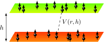
Figure 1: Schematic representation of the bilayer dipolar bosonic model. Particles obeying Bose-Einstein statistics are confined in two parallel layers. The dipoles are pinned perpendicularly to the layers’ planes and parallel to each other, yielding entirely repulsive on-plane interactions and partially attractive out-of-plane interactions.

In the following, we focus on a system of dipolar Bose gases confined in a bilayer geometry in continuous space, with the dipole orientation pinned perpendicular to the planes, as sketched in Fig. 1. This system is similar to the one studied in Ref. Terentjev and Shevchenko (1999), which pointed out the presence of entrainment between the superfluid currents of two charged superfluids in a bilayer configuration. The relative strength of interspecies interactions as compared to intraspecies ones can be tuned by changing the distance between the two layers. As it will be shown later in Fig. 3, for an extended range of this control parameter, the superfluid drag can reach very large values. Dipolar particles in a bilayer configuration are particularly advantageous under a variety of aspects. Confining the molecules in a two-dimensional geometry and imposing a repulsive dipolar interaction strongly reduces the detrimental two-body chemical reactions Ni et al. (2010). At the same time it allows to exploit the anisotropy of the dipolar interaction, which is partially attractive between particles on different layers. Introducing the distance $h$ between the two layers, the interaction between two particle of mass $m$ and dipole moment $d$ on different layers can be written as

$$V(r,h)=d^{2}\frac{r^{2}-h^{2}}{(r^{2}+h^{2})^{5/2}},$$ (24)

where $r$ is the relative distance in the plane of motion. For dipolar gases, it is very useful to introduce the characteristic length $r_{0}=md^{2}/\hbar^{2}$. The various regimes of the system are characterised by the interlayer parameter $h/r_{0}$ and the in-layer parameter $n_{i}r_{0}^{2}$, with $n_{i}$ the single layer density. Static and dynamic properties of this system were recently investigated in Macia et al. (2014); Astrakharchik et al. (2016). In particular, it has been found that a transition from two coupled superfluid (atomic phase) to a pair superfluid (molecular phase) takes place when the attractive interaction is strong enough. We will show that, by approaching the transition point while remaining in the atomic phase, the drag superfluidity becomes prominent.

To recover the description of Eq. (5), we point out that miscibility is here to be intended with respect to the position of the particles projected in the direction orthogonal to the layers’ planes. Dipolar Bose gases in a double layer configuration do not show any phase separation Macia et al. (2014). This is intuitive, since any potential with $V(q)|_{q=0}\leq 0$ (in momentum space) admits a bound state in $2D$. (The interlayer potential 24 has the peculiarity to have $V(q)|_{q=0}=0$, which makes the bound and scattering states of the system at weak coupling rather peculiar Klawunn et al. (2010)). The dipolar bilayer Bose gas is moreover the first example of a two component Bose gas which can form pairs without collapsing (i.e. forming clusters) Macia et al. (2014) as it occurs, e.g., in mixtures with contact interaction only.

Besides serving as a testbed for the numerical study of the superfluid drag in a homogeneous geometry and being a new system showing the AB physics, the dipolar bilayer configuration can represent one of the best-case scenarios for the experimental observation of the presence of superfluid drag. Recent experiments using dipolar molecules consisting of two atoms of Erbium-168 demonstrated the availability of condensates with large magnetic moments, up to $r_{0}\approx 1600\,{\rm a}_{0}$, with ${\rm a}_{0}$ the Bohr radius Frisch et al. (2015). This value is still almost one order of magnitude smaller with respect to the typical wavelength of the lasers used to confine the Er₂ molecules in arrays of 2D layers. Experiments on stable polar Na-K molecules Will et al. (2016), which sport much larger $r_{0}$, may help in overcoming this problem. The recent proposal of sub-wavelength confinement Nascimbene et al. (2015) may further stretch the experimentally accessible range of values of $h/r_{0}$, albeit it is not of easy implementation for dipolar molecules. Therefore, experimental realisation of a bilayer system of strongly interacting dipolar superfluids is reasonably within reach of current or near-future technology.

We study the system by means of diffusion QMC, which allows us to extract both the thermodynamics and the low energy spectrum of the system. Diffusion QMC is based on solving the Schrödinger equation in imaginary time, thus projecting out the ground state of the system (for a general introduction on the method see, e.g., Boronat and Casulleras (1994)). The contributions of the excited states are exponentially suppressed and the ground-state energy is recovered in the limit of long propagation time. The simulations are performed for $60$ particles with the same parameters as in Refs. Macia et al. (2014); Astrakharchik et al. (2016). For some quantities, this number of particles is sufficiently large to be close to the thermodynamic limit; for some others, residual finite-size corrections must be taken into account, as it will be explained in more details later.

In this framework, a number of observables of interest can be obtained in a straightforward way. The value of the gap $\Delta$ and of the spin susceptibility $\chi_{s}$ are obtained from the dependence of the ground-state energy on the polarisation $P=(N_{1}-N_{2})/N$. The latter is tuned by moving particles from layer $1$ to layer $2$ while keeping the total number of particles $N=N_{1}+N_{2}$ constant. In the limit of small polarisation $P$, the energy can be expanded as

$$E(P)=E(0)+N\Delta\cdot P+N\frac{n}{2\chi_{s}}\cdot P^{2}.$$ (25)

In the gapless phase ($\Delta=0$) the dependence on the polarisation is quadratic, while in the gapped phase it is linear. Similarly, the compressibility $\kappa_{d}$ at $T=0$ can be obtained from the volume dependence of the energy for an unpolarised gas,

$$\kappa_{d}^{-1}=-\mathcal{V}\left(\frac{\partial^{2}E}{\partial\mathcal{V}^{2}}\right),$$ (26)

where $\mathcal{V}$ is the $D$ dimensional volume of the system ($\mathcal{V}=L^{2}$ in the $2D$ geometry at hand).

The study of structure factors provides a way of accessing the dynamic properties of the system. We use the technique of pure estimators Liu et al. (1974); Casulleras and Boronat (1995) to compute the intermediate scattering function

$$S_{\alpha\beta}({\bf k},\tau)=\frac{1}{N}\left\langle\rho_{\alpha}({\bf k},\tau)\rho_{\beta}(-{\bf k},0)\right\rangle,$$ (27)

with $\rho_{\alpha}({\bf k},\tau)=\sum_{j}^{N_{\alpha}}\exp\{-i{\bf k}\cdot{\bf r}_{j\alpha}(\tau)\}$ and ${\bf r}_{j\alpha}$ the position of particle $j$ in layer $\alpha$. The intermediate scattering function provides information on the correlations in imaginary time $\tau$ and is the main ingredient to compute the static structure factor $S_{\alpha\beta}({\bf k})\equiv S_{\alpha\beta}({\bf k},0)$. We consider a balanced system with $N_{A}=N_{B}$ and study the symmetric and antisymmetric structure factors,

$$S_{d(s)}(k)=S_{11}(k)\pm S_{12}(k),$$ (28)

corresponding to the density and spin channels of the discussion above, respectively. The compressibility and the spin susceptibility can be compared to the respective static structure factors in the low momentum limit, in order to verify the sum rules. The structure factors further provide information on the excitation spectra: their long imaginary time asymptotic behaviour can be fitted to an exponential decay of the form

$$S_{d(s)}({\bf k},\tau)\sim Ze^{-\omega_{d(s)}(k)\tau}.\qquad(\tau\to\infty)$$ (29)

When phononic excitations are present, $\omega_{d(s)}(k)$ is linear for small momenta, with the slope directly related to the speeds of sound of the density and spin channels, respectively, through $\hbar\omega_{d(s)}(k)\simeq c_{d(s)}k$.

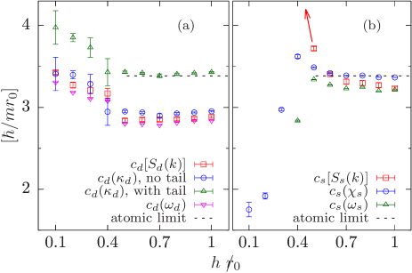
Figure 2: Speeds of sound as a function of interlayer spacing $h$ for $nr_{0}^{2}=1$, as extracted from different observables. (a) Speed of sound of the density mode, $c_{d}$. (b) Speed of sound of the spin mode, $c_{s}$. The Feynman method makes use of the static structure factor $S(k)=\hbar k/(2mc)$, computed at the smallest $k$ compatible with periodic boundary conditions. The speeds $c_{\alpha}[S_{\alpha}(k)]$, with $\alpha=\{d,s\}$ the channel index, are computed with this method. The data show that the f-sum rule is exhausted by the phonon mode in the density channel, whereas this does not hold in the spin channel, the arrow indicating the divergence of $c_{s}[S_{s}(k)]$. The speeds $c_{\alpha}(\omega_{\alpha})$, computed from the excitation spectrum, assume a linear phononic dispersion relation $\omega(k)=ck$ with $\omega_{\alpha}(k)$ obtained from Eq. (29). The speeds $c_{d}(\kappa_{d})$ and $c_{s}(\chi_{s})$ are computed from $mc_{d}^{2}=n\kappa_{d}^{-1}$ and $mc_{s}^{2}=n\chi_{s}^{-1}$, with $\kappa_{d}$ and $\chi_{s}$ obtained from Eqs. (26) and (25), respectively. The speed of sound in the atomic limit coincides in the two channels. It is obtained from standard thermodynamic relations using the equation of state $E(nr_{0}^{2})$ (taken from Ref. Astrakharchik et al. (2007)) of a single layer system with half the density of the bilayer system.

It is instructive to show that, in a gapless system without the drag, exactly the same information on the speeds of sound can be recovered from the static structure factors $S_{d,s}(k)$, the low-momentum excitation spectra $\omega_{d,s}(k)$, the compressibility $\kappa_{d}$ and the susceptibility $\chi_{s}$. The speeds of sound obtained from the different methods are shown in Fig. 2 for the density (a) and spin (b) modes. The density mode is gapless for any value of the interlayer separation $h$. The speed of sound of this channel, as obtained from structural, energetic and thermodynamic quantities, always yields compatible values throughout the explored range of $h$. Finite-size effects reduce the speed of sound, which for large $h$ (decoupled layers) appears to lie below its asymptotic value. The latter is obtained from the equation of state of a model with a single species at half the density (so called “atomic” limit). In the computations, the dipolar interaction potential was truncated at a distance equal to half the size of the simulation box. By adding the missing “tail” correction to the compressibility, it is possible to recover correct atomic limit asymptotics, as shown in the figure. The situation is quite different for the spin channel, where the gap opens for $h/r_{0}\lesssim 0.35$ and different methods cannot be consistent in that parameter range. For large values of the interlayer separation, $h/r_{0}\gtrsim 0.6$, we recover once again the atomic limit and different quantities are consistent with one another. Manifestly, it is not the case for parameter range $0.35\lesssim h/r_{0}\lesssim 0.6$, which still corresponds to a gapless phase but is in the vicinity of the transition point. In this region there is no consistency between the speeds of sound obtained with different methods and, importantly, the f-sum rule is not satisfied. The reason for this is appearance of the superfluid drag which we analyse in more details below. It is interesting to note that the finite-size effects are more pronounced in the density mode compared to the spin mode. One way to understand this is that the spin mode probes the response to the polarisation, which does not change the system volume, while the density (compression) mode is the response to a change in volume. The tail correction, being sensitive to the change of the volume, is able to account for the finite-size discrepancy.

Finally, in order to directly probe the superfluidity properties of the system, we introduce the winding number related to species $\alpha$,

$${\bf W}_{\alpha}(\tau)=\sum_{i(\alpha)=1}^{N/2}\int_{0}^{\tau}d\tau^{\prime}\frac{d{\bf r}_{i(\alpha)}(\tau^{\prime})}{d\tau^{\prime}},$$ (30)

where $i(\alpha)$ indexes particles belonging to species $\alpha$ only. Taking the limit of long propagation time, the statistics of the winding numbers are related to the superfluid densities. In particular, we evaluate the symmetric and antisymmetric combinations

$$\rho_{1}+\rho_{2}\pm 2\rho_{12}=\lim_{\tau\to\infty}\frac{\langle[{\bf W}_{1}(\tau)\pm{\bf W}_{2}(\tau)]^{2}\rangle}{2N\tau}.$$ (31)

According to Eq. (IV), when the plus sign is considered, the quantity above is an estimator of the total superfluid density of the system, $\rho_{T}$. In our zero temperature simulation, this quantity is always compatible with the total mass density, as it should be in continuous space, and in contrast with the low total superfluidity observed in lattice simulations. When the minus sign is considered, on the other hand, we directly probe the magnitude of the superfluid drag. This observable asymptotically attains the value $\rho_{T}$ in the non interacting ($h\to\infty$) limit. In the symmetric mixture case, borrowing the same notations of Sec. III, this quantity reduces to $(\rho-\rho_{12})/nm$, and is reported in Fig. 3. For low interactions (large $h$), it is compatible with unity and drops to zero as interactions are ramped up. This corresponds to $\rho_{12}=\rho_{T}/4$, i.e., with bound (23). It must be noted that, for $h<h_{c}\approx 0.35r_{0}$Macia et al. (2014), the system enters the molecular phase, so that not all the drop in $\rho-\rho_{12}$ can be ascribed to an increase of the drag, but one must also keep into account the emergence of the molecular condensate. Indeed, the description we put forward holds only as long as the system is still in the atomic phase. Interestingly, the saturation of the bound (23) (or, alternatively $m^{*}\rightarrow 2m$) appears to coincide with the transition to the molecular phase in which bound state physics start dominating.

Figure 3: The quantity $(\rho-\rho_{12})$, extracted from diffusion QMC data using different estimators. The direct winding number estimator (diamonds and dashed line to guide the eye) is compared with indirect estimators. The latter make use of the relations derived in the quantum hydrodynamic model of Sec. III (cf. also Eq. (32)). The data sets are in satisfactory agreement with one another, with the exception of the estimator $c_{s}^{2}[S_{s}(k)]\chi_{s}$, which tends to diverge as the molecular phase is approached (shaded region). The origin of the errorbars and of remaining finite-size effects are discussed in the main text.

By independently measuring $S_{s}(k)$, $\chi_{s}$ and $\omega_{s}$ (hence $c_{s}$), we can show that the usual Bijl-Feynman approximation is not applicable to systems in the presence of the superfluid drag. To this end, we use Eqs. (12)-(13) to express $(\rho-\rho_{12})$ in terms of the observables listed above, and then compare it with the direct winding number measurement. Figure 3 reports the data corresponding to the three independent expressions

$$\frac{\rho-\rho_{12}}{nm}=\frac{4mS^{2}_{s}(k)}{\chi_{s}k^{2}}=2\frac{c_{s}(\omega_{s})S_{s}(k)}{k}=c_{s}^{2}(\omega_{s})\chi_{s},$$ (32)

where we are indicating by $c_{s}(\omega_{s})$ the speed of sound in the spin channel as extracted from the fit to Eq. (29). The data show fair agreement among the above expressions and between them and the direct measurement of $\rho-\rho_{12}$. A notable exception are the data for $c_{s}^{2}[S_{s}(k)]/\chi_{s}$, where $c_{s}[S_{s}(k)]$ is the speed of sound in the spin channel, computed as if Bijl-Feynman relation held. We observe that this expression leads to the wrong behaviour in the region where $\rho-\rho_{12}$ differs from one, i.e., where the drag effect is more prominent.

In both Figs 2 and 3, the errobars in the quantities extracted from the static structure factor and the winding number come from statistical averaging. Spectral frequency, compressibility and susceptibility have additional contributions to the error due to the use of fitting procedures, Eqs. (25) and (29). The errors are effectively increased in some of the results, due to cancellation of opposite trends as a function of $h$. The finite-size effects are important for a quantitative agreement, as can be seen from Fig. 2a. It is not obvious that different quantities have similar finite-size correction, which might eventually be responsible for some remaining differences between various estimations in Fig. 3.

V Dynamic stability

Given the recent advances in measuring the spin superfluidity and its critical dynamics, we devote the final section to explore the consequences of the presence of a superfluid drag term on such phenomena. Both long living spin oscillations Bienaimé et al. (2016) and critical spin superflow Kim et al. (2017) for Bose-Bose mixtures as well as for Fermi-Bose superfluid mixtures Delehaye et al. (2015) have been measured in the weakly interacting regime. The agreement with the available estimates Castin et al. (2015); Abad et al. (2015) is reasonable but rather far from being quantitative.

In the following, we determine the critical relative velocity required to trigger the dynamical instability of a binary mixture of superfluids at zero temperature. To this end, we generalise Eqs. (2) and (5) and the results of Refs. Kravchenko and Fil (2008, 2009); Abad et al. (2015) by considering the energy functional

$$E[ n_{1},n_{2},\phi_{1},\phi_{2}]=$$

$$=\int\left\{\frac{\hbar^{2}}{2}\sum_{\alpha}\left[\frac{m_{\alpha}n_{\alpha}-\rho_{12}}{m_{\alpha}^{2}}(\nabla\phi_{\alpha})^{2}\right]\right.$$

$$\left.\quad+\frac{\rho_{12}}{m_{1}m_{2}}\nabla\phi_{1}\cdot\nabla\phi_{2}+e(n_{1},n_{2})\,\right\}d^{D}x$$ (33)

with $e(n_{1},n_{2})$ the internal energy density. We subtracted $\rho_{12}$ from the diagonal kinetic terms, so that the condition (3) on the total density is automatically satisfied. Considering $n_{\alpha}$ and $\phi_{\alpha}$ as conjugate variables, the Hamilton equations $m_{\alpha}\partial_{t}n_{\alpha}=\delta E/\delta\phi_{\alpha}$ and $m_{\alpha}\partial_{t}\phi_{\alpha}=-\delta E/\delta n_{\alpha}$, yield (implying $\alpha\neq\beta$)

$$\partial_{t}n_{\alpha}=-\nabla(n_{\alpha}{\bf v}_{\alpha})+m_{\alpha}^{-1}\nabla\left[\rho_{12}({\bf v}_{\alpha}-{\bf v}_{\beta})\right],$$ (34)

$$\partial_{t}{\bf v}_{\alpha}=-\nabla\frac{v_{\alpha}^{2}}{2}+\nabla\left[\frac{\eta_{\alpha}}{m_{\alpha}}\left(\frac{v_{\alpha}^{2}}{2}-{\bf v}_{1}\cdot{\bf v}_{2}\right)\right]-\frac{\nabla\mu_{\alpha}}{m_{\alpha}},$$ (35)

where ${\bf v}_{\alpha}=(\hbar/m)\nabla\phi_{\alpha}$ are the superfluid velocities, $\mu_{\alpha}=\partial\epsilon/\partial n_{\alpha}$ the chemical potentials and we defined $\eta_{\alpha}\equiv\partial\rho_{12}/\partial n_{\alpha}$, implicitly assuming that $\rho_{12}$ is a well-behaved function of the densities. The previous system of hydrodynamic equations is satisfied by a steady state solution of uniform velocity, matter and drag fields, such that all gradient terms vanish. With a slight change of notation, we perturb about this solution by expanding the density and velocity fields as

$$n_{\alpha}\mapsto\bar{n}_{\alpha}+n_{\alpha}e^{i({\bf qr}-\omega t)},$$ (36)

$${\bf v}_{\alpha}\mapsto\bar{{\bf v}}_{\alpha}+{\bf v}_{\alpha}e^{i({\bf qr}-\omega t)},$$ (37)

and only keep the first order in the fluctuations, whereas, since it is already small with respect to $n_{\alpha}m_{\alpha}$, we only keep the zero-th order in $\rho_{12}$. Substituting these expansions into Eqs. (34)-(35), we obtain

$$n_{\alpha}[\omega-\bar{{\bf v}}_{\alpha}\cdot{\bf q}]=\bar{n}_{\alpha}{\bf v}_{\alpha}\cdot{\bf q}-\frac{\rho_{12}}{m_{\alpha}}({\bf v}_{\alpha}-{\bf v}_{\beta})\cdot{\bf q},$$ (38)

$${\bf v}_{\alpha}[\omega-\bar{{\bf v}}_{\alpha}\cdot{\bf q}]=\frac{{\bf q}}{m_{\alpha}}\sum_{\gamma=1,2}\mu_{\alpha\gamma}n_{\gamma},$$ (39)

where we abbreviated $\mu_{\alpha\beta}\equiv\partial\mu_{\alpha}/\partial\bar{n}_{\beta}$ (hence $\mu_{12}=\mu_{21}$, as expected by the symmetry of interactions). In Eq. (39), we neglected the term proportional to $\eta_{\alpha}$, as the leading order is $O(\rho_{12}n_{\alpha},\rho_{12}v_{\alpha})$, and the zero-th order, homogeneous by hypothesis, vanishes under spatial differentiation.

Eliminating $n_{\alpha}$ and $v_{\alpha}$ in the system of equations (38)-(39) leads to

$$\left\{\Omega_{1}^{2}\Omega_{2}-\left[c_{1}^{2}\Omega_{2}-\rho_{12}\left(\frac{\mu_{11}\Omega_{2}}{m_{1}^{2}}-\frac{\mu_{21}\Omega_{1}}{m_{1}m_{2}}\right)\right]q^{2}\right\}\left\{\Omega_{2}^{2}\Omega_{1}-\left[c_{2}^{2}\Omega_{1}-\rho_{12}\left(\frac{\mu_{22}\Omega_{1}}{m_{2}^{2}}-\frac{\mu_{12}\Omega_{2}}{m_{1}m_{2}}\right)\right]q^{2}\right\}=$$

$$\qquad\qquad\qquad\qquad\qquad\qquad=q^{4}\left[\bar{n}_{1}\frac{\mu_{12}\Omega_{2}}{m_{1}}-\rho_{12}\left(\frac{\mu_{12}\Omega_{2}}{m_{1}^{2}}-\frac{\mu_{22}\Omega_{1}}{m_{1}m_{2}}\right)\right]\left[\bar{n}_{2}\frac{\mu_{21}\Omega_{1}}{m_{2}}-\rho_{12}\left(\frac{\mu_{21}\Omega_{1}}{m_{2}^{2}}-\frac{\mu_{11}\Omega_{2}}{m_{1}m_{2}}\right)\right],$$ (40)

where we set $\Omega_{\alpha}\equiv\omega-\bar{{\bf v}}_{\alpha}\cdot{\bf q}$ and $c_{\alpha}^{2}\equiv\bar{n}_{\alpha}\mu_{\alpha\alpha}/m_{\alpha}$, the latter being the speed of sound of a single superfluid. We also define

$$c_{12}^{4}\equiv\frac{\bar{n}_{1}\bar{n}_{2}}{m_{1}m_{2}}\mu_{12}^{2},$$ (41)

which has got the dimension of a speed and measures the strength of inter-species contact interactions. By assuming a linear dispersion $\omega=Cq$, the one above is a sixth order equation for the speed of sound $C$ of the mixture, which determines its stability. In particular, the presence of complex roots flags a dynamical instability. By setting $\rho_{12}=0$, Eq. (40) reduces to the problem of the stability of a mixture interacting only via contact interactions, which was studied in depth in Abad et al. (2015).

This equation simplifies considerably when rewritten in a symmetric frame of reference (SFR) in which $v/2=\bar{{\bf v}}_{1}\cdot{\bf q}=-\bar{{\bf v}}_{2}\cdot{\bf q}$, so that the projection of the relative velocity of the two fluids along ${\bf q}$ is simply $v$. When $n_{1}m_{1}=n_{2}m_{2}$, this choice corresponds to the frame of reference of the centre of mass of the system. A brief analysis of the case $v=0$ is reported in the Appendix A.

V.1 Symmetric mixture

Some insight into the dynamic stability of the mixture can be gained by considering a $\mathbb{Z}_{2}$ symmetric mixture, in which $\bar{n}_{\alpha}=\bar{n}$, $m_{\alpha}=m$ and $\mu_{\alpha\alpha}$ are the same for both species (hence also the speeds of sound coincide, $c_{\alpha}=c$). The stability equation (40) then simplifies to a biquadratic equation whose roots can be readily calculated. Restricting to positive relative velocities, the condition that the two-fluid speed of sound be real then yields the critical relative velocities for the stability of the mixture:

$$\frac{v_{{\rm c}1}}{c}=2\sqrt{1-\frac{c_{12}^{2}}{c^{2}}},\quad\frac{v_{{\rm c}2}}{c}=2\sqrt{\left(1+\frac{c_{12}^{2}}{c^{2}}\right)\left(1-4\frac{\rho_{12}}{\rho_{T}}\right)}.$$ (42)

For $c_{12}=\rho_{12}=0$, the system is unstable for $v>2c$, confirming the results of Refs. Kravchenko and Fil (2008, 2009); Castin et al. (2015); Abad et al. (2015). When the relative velocity $v$ lies within $v_{{\rm c}1}$ and $v_{{\rm c}2}$, the mixture becomes unstable, as schematically shown in Fig. 4.

It is worth reminding that the stability analysis presented here is valid within hydrodynamics, i.e., assuming a linear dispersion relation. The inclusion of non-linear terms can give rise to finite momentum instabilities above the upper critical velocity, as it was pointed out in the case of a Bose-Bose mixture without superfluid drag Ishino et al. (2011). Whether such finite momentum instability occurs in the same way also in presence of AB corrections is beyond the scope of the present paper and it will be discuss elsewhere. Nevertheless for large enough drag,

$$\frac{\rho_{12}}{\rho_{T}}>\frac{1}{4}\left[1-\frac{c^{2}-c_{12}^{2}}{c^{2}+c_{12}^{2}}\right].$$ (43)

the lower critical velocity is $v_{{\rm c}2}$, which depends on the entrainment: in this regime, it should be possible observe a shift in the onset of the dynamical instability. In particular for $\rho_{12}=\rho_{T}/4$, i.e., when the condition (23) is saturated and the spin speed of sound vanishes, the mixture is unstable already at vanishing relative velocities.

For completeness, we compare the critical velocities for the dynamic stability (42) with the speeds of sound of the density and spin modes, Eqs. (9)-(10), respectively, which provide the critical velocity for the energetic (Landau) instability. With the notation of this section, they read

$$c_{d}^{2}=c^{2}+c_{12}^{2},\qquad c_{s}^{2}=\left(1-4\frac{\rho_{12}}{\rho_{T}}\right)(c^{2}-c_{12}^{2}),$$ (44)

and they are also reported in Fig. 4. Although it occurs at a lower critical velocity, the energetic instability would not obfuscate the dynamical instability. A counterflow experiment would only slightly trigger the Landau instability, which in any case would develop much more slowly than the dynamical one. Experimental methods based on the generation of soliton trains Hoefer et al. (2011); Hamner et al. (2011); Kim et al. (2017) were shown to be able to cleanly identify dynamical instabilities of the kind discussed in this section.

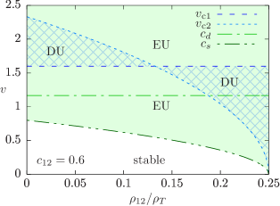
Figure 4: Stability diagram for a superfluid mixture with contact interactions such that $c_{12}=0.6$ and all speeds expressed in units of $c$. The spin speed of sound $c_{s}$ is always below the density speed of sound $c_{d}$ (cf. Eq. (44)). The former delimits the energetically unstable (EU) region (solid filling). The dynamically unstable (DU) region (grid filling) lies between the critical velocities $v_{{\rm c}1}$ and $v_{{\rm c}2}$, cf. Eq. (42). The threshold relative velocities for both EU and DU vanish for $\rho_{12}/\rho_{T}=1/4$.

VI Conclusions

In the present work, we studied the physics of a superfluid mixture in the presence of current-current interactions, which lead to the so-called Andreev-Bashkin effect (AB). Our minimal quantum hydrodynamic theory highlights the consequences of the presence of the superfluid drag $\rho_{12}$ as an off-diagonal coefficient of the superfluid density matrix. In particular, for $\mathbb{Z}_{2}$ symmetric mixtures, in which the density and spin modes decouple, we predict the density channel to remain unaffected; the spin channel, on the other hand, exhibits corrections of linear order in $\rho_{12}$ in both static quantities, such as the spin susceptibility $\chi_{s}$, and in dynamic quantities, such as the speed of sound of the spin mode, $c_{s}$. A prominent consequence of these corrections is that Bijl-Feynman theory, relating $c_{s}$ to $\chi_{s}$, is no longer satisfied in the presence of AB corrections, as shown by Eq. (13). In light of these results, we identify the speeds of sound and the susceptibilities as being the most promising observables in order to experimentally study the AB effect. The quantum hydrodynamic theory further provides an upper bound to the value of $\rho_{12}$, which must remain less than a fourth of the total superfluid density $\rho_{T}=\rho_{1}+\rho_{2}+2\rho_{12}$ (alternatively, in the language of the effective mass, $m^{*}\leq 2m$). The same bound appears also in the path integral formulation of superfluid densities, extended to a mixture of two superfluids, as well as a limiting case of the critical velocity (42) for the dynamic stability of the mixture.

The minimal toy model employed in Sec. III also gives insight on low but finite temperature properties such as the specific heat, which is expected to depend on the drag through a factor $c_{s}^{-D}$ in $D$ dimensions. In general, finite temperature has a detrimental effect on the possibility of observing AB-related phenomena Terentjev and Shevchenko (1999); Fil and Shevchenko (2004), due to the reduction of the superfluid density and to the emergence of dissipative drag between the two components. In this respect, the quantities we suggest to focus on to find experimental evidence of the presence of entrainment are much more suitable than trying to directly detect the current induced by one component on the other. It is worth mentioning that a recent experiment Fava et al. (2017) was able to record the dynamics of both superfluid and normal fractions of a weakly interacting Bose-Bose mixture, as well as the finite temperature polarisabilities. We believe that experiments such as this one pave the way towards the detection of subtle superfluid effects such as the AB drag.

As a check on the predictions of the quantum hydrodynamic model, we numerically investigated a system of $\mathbb{Z}_{2}$ symmetric bilayer dipolar bosons, with repulsive interactions within each layer and partially attractive interactions between the two layers. The diffusion quantum Monte Carlo method allows the simultaneous measurement of several observables, separately on the density and spin channels. By inverting the theoretical relations between the static and dynamic observables, and the superfluid drag, we can compare indirect estimators of $\rho_{12}$ with the direct estimator based on the winding numbers. Figure 3 shows a good agreement between direct and indirect measurements of $(\rho-\rho_{12})/nm$. A notable exception is when one extracts the speed of sound of the spin channel using the Bijl-Feynman relation, which, as aforementioned, breaks down if $\rho_{12}\neq 0$.

We finally analysed the stability of the superfluid mixture. The condition for the onset of the (static) phase separation instability only involves the density channel, and hence is not modified by $\rho_{12}$. On the other hand, when the two fluids are put in relative motion, for some values of the relative velocity the mixture becomes dynamically unstable. The critical velocities, reported in Eqs. (42), carry a dependence on the superfluid drag. This result extends the previous ones Kravchenko and Fil (2008, 2009); Abad et al. (2015); Castin et al. (2015) which analysed a system with contact interactions only.

In the light of recent experimental works Frisch et al. (2015); Delehaye et al. (2015); Roy et al. (2017), it is reasonable to claim that, albeit the AB is expected to be a subdominant effect, it may still be within reach of current experimental technology. It further opens up the game to interesting new phenomenological effects: for instance, if one is able to phase imprint a vortex on one species of the mixture, one may expect at least part of the vorticity to be transferred in a dissipationless fashion to the other species. This sympathetic stirring of a superfluid mixture could become a useful tool in the study of vortex dynamics in superfluid mixtures. The stability conditions we put forward in Sec. V and Appendix A may also have consequences in astrophysics, and in particular on the rotation profiles of neutron star cores Kobyakov and Pethick (2017).

Appendix A Quantum hydrodynamics for a non-symmetric mixture

We consider Eq. (5) in the more general case in which the two species are not symmetric ($\rho_{11}\neq\rho_{22}$, $\alpha_{11}\neq\alpha_{22}$ and $m_{1}\neq m_{2}$). Hamilton equations lead to the equation of motion for phase fluctuations,

$$\ddot{\phi_{i}}(x)=-\left(\frac{\hbar^{2}}{m_{i}m_{l}}\alpha_{il}\rho_{lj}\right)k^{2}\phi_{j}(x),$$ (45)

and the quantity in parentheses can be identified with the matrix $C_{ij}$ of the squared speeds of sound.

Written with respect to an eigenbasis of $C_{ij}$, the system exhibits two non-interacting modes which obey a linear dispersion relation $\omega_{\pm}=c^{2}_{\pm}k^{2}$. The speeds of sound $c_{\pm}^{2}$, eigenvalues of $C_{ij}$, generalise Eqs. (9)-(10). Obviously, contrary to Sec. III, the two independent modes are not “pure” density and spin channels, due to the lack of $\mathbb{Z}_{2}$ symmetry.

In terms of the coefficients of matrix $C_{ij}$, the eigenspeeds of sound read

$$c^{2}_{\pm}= \frac{C_{11}+C_{22}}{2}$$

$$\pm\frac{1}{2}\sqrt{(C_{11}+C_{22})^{2}-4(C_{11}C_{22}-C_{12}C_{21})},$$ (46)

The system is stable as long as $c_{\pm}^{2}$ are positive, which leads to the inequality $C_{11}C_{22}-C_{12}C_{21}>0$, or, in terms of the model’s coefficients,

$$(\alpha_{11}\alpha_{22}-\alpha_{12}^{2})(\rho_{11}\rho_{22}-\rho_{12}^{2})>0$$ (47)

The second factor in this equation is always positive, thanks to the bound on the magnitude of the superfluid drag (cf. discussion leading to Eq. (23)). We thus obtain a condition on the strength of the density-density interactions, namely $(\alpha_{11}\alpha_{22}-\alpha_{12}^{2})>0$, thus recovering the well known criterion for the onset of the phase separation instability Pitaevskii and Stringari (2016).

Appendix B Relation between winding numbers and superfluid densities

Following Pollock and Ceperley (1987), we imagine a slab of fluid sandwiched between two parallel boundaries, moving with respect to the fluid with velocity ${\bf v}$. We can write the density matrix of a two-species system in a frame comoving with the boundaries as

$$\rho_{v}(R,R^{\prime},\beta)=\langle R^{\prime}|e^{-\beta H_{v}}|R\rangle,$$ (48)

$$H_{v}=\sum_{\alpha=\{1,2\}}\sum_{j=1}^{N_{\alpha}}\frac{({\bf p}_{j}-m_{\alpha}{\bf v})^{2}}{2m_{\alpha}}+V,$$ (49)

where $V$ comprises both inter- and intra-species interactions, both assumed to depend on positions only. (Greek indices identify the species, while Latin indices count particles). The change in total momentum in the frame of reference of the boundaries is due to the response of the normal component $\rho_{N}$ of the fluid, hence, calling $\rho_{0}=\rho_{v=0}$, the density matrix in the frame of rest of the fluid,

$$\frac{\rho_{N}}{\rho_{0}}(N_{1}m_{1}+N_{2}m_{2}){\bf v}=\frac{\rho_{N}}{\rho_{0}}M{\bf v}=\langle{\bf P}_{v}\rangle=\frac{\operatorname{tr}[{\bf P}_{v}\rho_{v}]}{\operatorname{tr}[\rho_{v}]},$$ (50)

and is equal to one minus the total superfluid fraction, which can then be written in terms of the variation of the free energy as

$$\frac{\rho_{T}}{\rho_{0}}=\frac{\partial\mathcal{F}_{v}}{\partial(\frac{1}{2}Mv^{2})}.$$ (51)

We can write the density matrix in Fourier space and relate the density matrix $\rho_{0}$ in the frame of rest to $\rho_{v}$,

$$\rho_{v}=\exp\left\{i{\bf v}\cdot\sum_{\alpha,j}(r_{j\alpha}-r^{\prime}_{j\alpha})m_{\alpha}\right\}\tilde{\rho}_{0}.$$ (52)

Under periodic permutations of the particles,

$$\rho_{v}=e^{i{\bf v}\cdot m_{1}{\bf W_{1}}L}e^{i{\bf v}\cdot m_{2}{\bf W_{2}}L}\tilde{\rho}_{0},$$ (53)

whence

$$e^{-\beta\Delta\mathcal{F}_{v}} =\frac{1}{\mathcal{Z}}\int\tilde{\rho}_{0}\,e^{i(m_{1}{\bf W_{1}}+m_{2}{\bf W_{2}})\cdot{\bf v}L}$$

$$=\langle e^{i(m_{1}{\bf W_{1}}+m_{2}{\bf W_{2}})\cdot{\bf v}L}\rangle.$$ (54)

Expanding to leading order the previous expression, one finally gets

$$\Delta\mathcal{F}_{v}=\frac{1}{2}\frac{v^{2}L^{2}}{d\beta}\langle(m_{1}W_{1}+m_{2}W_{2})^{2}\rangle$$ (55)

and, using Eq. (51) and $\rho_{0}=ML^{-d}$,

$$\rho_{s}^{tot} =\frac{L^{2-d}}{d\beta}\langle(m_{1}W_{1}+m_{2}W_{2})^{2}\rangle,$$ (56)

yielding Eq. (IV).