Stabilization of the response of cyclically loaded lattice spring models with plasticity

Abstract

This paper develops an analytic framework to design both stress-controlled and displacement-controlled $T$-periodic loadings which make the quasistatic evolution of a one-dimensional network of elastoplastic springs converging to a unique periodic regime. The solution of such an evolution problem is a function $t\mapsto(e(t),p(t))$, where $e_{i}(t)$ and $p_{i}(t)$ are the elastic and plastic deformations of spring $i,$ defined on $[t_{0},\infty)$ by the initial condition $(e(t_{0}),p(t_{0}))$. After we rigorously convert the problem into a Moreau sweeping process with a moving polyhedron $C(t)$ in a vector space $E$ of dimension $d,$ it becomes natural to expect (based on a result by Krejci) that the solution $t\mapsto(e(t),p(t))$ always converges to a $T$-periodic function. The achievement of this paper is in spotting a class of loadings where the Krejci’s limit doesn’t depend on the initial condition $(e(t_{0}),p(t_{0}))$ and so all the trajectories approach the same $T$-periodic regime. The proposed class of sweeping processes is the one for which the normals of any $d$ different facets of the moving polyhedron $C(t)$ are linearly independent. We further link this geometric condition to mechanical properties of the given network of springs. We discover that the normals of any $d$ different facets of the moving polyhedron $C(t)$ are linearly independent, if the number of displacement-controlled loadings is two less the number of nodes of the given network of springs and when the magnitude of the stress-controlled loading is sufficiently large (but admissible). The result can be viewed as an analogue of the high-gain control method for elastoplastic systems. In continuum theory of plasticity, the respective result is known as Frederick-Armstrong theorem.

The theoretical results are accompanied by analytic computations for instructive examples. In particular, we convert a specific one-dimensional network of elastoplastic springs into sweeping process which have never been explicitly addressed in the literature so far.

1 Introduction

The classical theory of elastoplasticity offers comprehensive results, commonly known as shakedown theorems, about the maximal magnitude of the applied loading (shakedown load limit) beyond which the response of elastoplastic material necessarily involves plastic deformation regardless of the initial distribution of stresses in the material, see (jirasek, , §10). In other words, shakedown theorems measure the distance between the current stress distribution in the material to a certain boundary (called yield surface) built of the spatially distributed elastic limits. The fundamental result by Frederick and Armstrong frederick says that, if the amplitude of a $T$-periodic loading exceeds the shakedown limit, then the stress distribution asymptotically approaches a unique $T$-periodic steady cycle which doesn’t depend on the initial stress distribution (uniqueness of the response). Frederick-Armstrong highlight that convergence to a unique cyclic state is guaranteed when the yield surface contains no lines of zero curvature (frederick, , p. 159). Assuming this or another restriction on the geometry of the yielding surface (such as von Mises, Tresca, or Mohr-Coulomb criteria), many authors computed the steady cycle by discretizing the problem spatially garcea ; Heitzer ; li and/or temporarily polizzotto ; ponter ; brazil , and by solving the associated minimization problems for the successive discrete states. Applications included the performance of various structures and metal matrix composites under cyclic loadings, see simplified ; weichert1 .

Aiming to design materials with better properties, there has been a great deal of work lately where a discrete structure comes not from an associated model of continuum mechanics, but from a certain microstructure formulated through a lattice of elastic springs crystal1 ; li1 (metals), polymer ; novel (polymers), JiaoPrior2 (titanium alloys), tissue ; natureb ; sva (biological materials). Despite of the fact that fatigue crack initialization in heterogeneous materials strongly depends on local micro-plasticity (see e.g. Blechman blechman ), the current literature features only numeric results about the dynamics of the lattices of elastoplastic springs. Important papers in this direction are e.g. Buxton et al buxton and Chen et al chen .

The goal of the present paper is to initiate the development of a qualitative theory of the lattices of elastoplastic springs and to offer an analogue of the Frederick-Armstrong theorem for such systems.

We stick to the setting of ideal plasticity (the stress of each spring is constrained within so-called elastic limits beyond which plastic deformation begins) and investigate the asymptotic distribution of the stresses $s(t)=(s_{1}(t),...,s_{m}(t))$ of a network of $m$ elastoplastic springs. Starting with a graph of $m$ connected elastoplastic springs, the paper takes Moreau’s approach moreau to write down the equation for stress $s_{i}$ of spring $i$ without any knowledge about plastic deformation of the spring and relying entirely on the geometry of the graph and elastic limits $[c_{i}^{-},c_{i}^{+}]$ of the springs. The plasticity is accounted through the $m$-dimensional parallelepiped-shaped constraint $C(t)$, whose boundary can be viewed as discretized yield surface, see Fig. 3. Beneficially for the performance of computational routines, Moreau concluded that the stress-vector $s(t)=(s_{1}(t),...,s_{m}(t))$ of springs is confined within a time-independent low-dimensional hyperplane $V$. It is also due to Moreau that external time-varying loadings enter the equations of dynamics through a time-varying vector $c(t)$ that acts as displacement of the parallelepiped $C$ (Fig. 3). The only obstacle towards practical implementation of the Moreau approach moreau in the context of spring network modeling is that moreau deals with abstract configuration spaces translated into practical quantities only for examples from dry friction mechanics. This paper clears this obstacle and fully adapts Moreau sweeping process framework to the modeling of networks of elastoplastic springs.

After a suitable change of variables that we rigorously incorporate in the next section of the paper, the equations of Moreau (Moreau sweeping process) can be formulated as

$$-y^{\prime}(t)\in N_{({C}+c(t))\cap V}(y(t)),\quad y(t)\in\mathbb{R}^{m},$$ (1)

where

$$N_{\mathcal{C}}(x)=\left\{\begin{array}[]{ll}\left\{\zeta\in\mathbb{R}^{n}:\langle\zeta,c-x\rangle\leqslant 0,\ {\rm for\ any}\ c\in{\mathcal{C}}\right\},&{\rm if}\ x\in{\mathcal{C}},\\ \emptyset,&{\rm if}\ x\not\in{\mathcal{C}}\end{array}\right.$$ (2)

is a normal cone to the set $\mathcal{C}$ at point $x$ and $V$ is a subspace of $\mathbb{R}^{m}$. For Lipschitz-continuous $t\mapsto c(t)$ (which we show to be the case when the external loading is Lipschitz-continuous) sweeping process (1) possesses usual properties of the existence and continuous dependence of solutions on the initial conditions, see e.g. Kunze and Monteiro Marques kunze .

When sweeping process (1) includes a vector field on top of the normal cone (so-called perturbed sweeping process), multiple results are available to stabilize the dynamics of a sweeping process. Important results in this direction are obtained in Leine and van de Wouw leine ; leine2 , Brogliato brogliato1 , and Brogliato-Heemels brogliato2 , Kamenskiy et al nahs .

As for the regular sweeping process (1), very limited tools to control the asymptotic response are currently available (in contrast to optimal control results developed e.g. in Colombo et al colombo ). The asymptotic behavior of sweeping process (1) with $T$-periodic excitation $t\mapsto c(t)$ was studied in Krejci Krejci1996 , who proved the convergence of solutions of (1) to a $T$-periodic attractor in the case $V=\mathbb{R}^{m}$, i.e. $(C+c(t))\cap V=C+c(t).$ If sweeping process (1) decomposes into a cross-product of several sweeping processes (1) with $m=1$, the global asymptotic stability can be concluded from the theory of Prandtl-Ishlinskii operators (Brokate-Sprekels brokate , Krasnosel’skii-Pokrovskii pokrov , Visintin visintin ). In the case of an arbitrary $T$-periodic polyhedron $t\mapsto(C+c(t))\cap V$, it looks possible to follow the ideas of Adli et al adly and obtain global asymptotic stability of a periodic solution by assuming that $g(t)$ lies strictly inside the normal cone $N_{(C+c(t))\cap V}(y)$ for at least one $y$ and $t\in[0,T]$. The present paper takes a different route and establishes convergence of solutions to a unique $T$-periodic regime in terms of the shape of the moving constraint $(C+c(t))\cap V$ only.

The paper is organized as follows. The next section rigorously formulates the system of laws of quasistatic evolution for a one-dimensional network of $m$ elastoplastic springs on $n$ nodes. In section 3 we construct the vector $c(t)$ and the hyperplane $V$ for arbitrary networks of elastoplastic springs of 1-dimensional nodes. We discover that the functions $g(t)\in V$ and $h(t)\perp V$ in the orthogonal decomposition of $c(t)$ (see Fig. 3) correspond to displacement-controlled and stress-controlled loadings respectively (as termed in simplified ). The achievement of Section 2 makes it possible to link the dynamics of networks of elastoplastic springs to the dynamics of sweeping processes.

In Section 4 we consider a general sweeping process with a moving set of a form $\cap_{i=1}^{k}(C_{i}+c_{i}(t))$, where $C_{i}$ are closed convex sets, and prove (Theorem 4.1) the convergence of all solutions to a $T$-periodic attractor $X(t)$. Section 4.2 (Theorem 4.3) sharpens the conclusion of Theorem 4.1 for the case when $\cap_{i=1}^{k}(C_{i}+c_{i}(t))$ is the polyhedron $\Pi(t)\cap V.$ Theorem 4.3 shows that even though $X(t)$ may consist of a family of functions, all those functions exhibit certain similar dynamics. Specifically, we prove that any two function $x_{1},x_{2}\in X$ reach (leave) any of the facets of $\Pi(t)\cap V$ at the same time. Section 4.3 (Theorem 4.4) reformulates the conclusion of Theorem 4.3 in terms of the sweeping process of a network of elastoplastic springs.

Section 5 introduces a class of networks of elastoplastic springs whose stresses converge to a unique $T$-periodic regime regardless of applied $T$-periodic loadings as long as the magnitudes of those loadings are sufficiently large. We begin Section 5 by addressing a general sweeping process in a vector space $E$ of dimension $d$ with a $T$-periodic polyhedral moving set with no connection to networks of springs. Theorem 5.1 of Section 5.1 states that the periodic attractor of such a sweeping process contains at most one non-constant solution, if normals of any $d$ different facets of the moving polyhedron $C(t)$ are linearly independent. Section 5.2 is the main achievement of this paper, where we introduce a class of networks of elastoplastic springs for which the condition of Theorem 5.1 can be easily expressed in terms of the magnitudes of the periodic loadings. We discovered (Theorem 5.2) that global stability of a unique periodic regime occurs when both displacement-controlled and stress-controlled loadings are large enough.

2 The laws of quasistatic evolution for one-dimensional networks of elastoplastic springs

We consider a one-dimensional network of $m$ elastoplastic springs with elongations $e_{k}+p_{k},$ $k\in\overline{1,m}$, where $e_{k}$ and $p_{k}$ are elastic and plastic components respectively. The bounds of the stress of spring $k$ are denoted by $[c_{k}^{-},c_{k}^{+}]$ and $a_{k}$ stays for the Hooke’s coefficient of this spring. Each spring connects two of $n$ nodes according to $e_{k}+p_{k}=\xi_{j_{k}}-\xi_{i_{k}}$, where $i_{k}$ and $j_{k}$ are the indices of the left and right nodes of spring $k$ respectively and $\xi_{i}$ is the displacement of node $i.$ So defined, the one-dimensional network of springs is an oriented graph on $n$ nodes, where the direction from $i_{k}$ to $j_{k}$ is viewed positive through $k\in\overline{1,m}.$

The paper investigates the evolution of the stresses under the influence of two types of loadings being displacement-controlled loading and stress-controlled loading.

2.1 Displacement-controlled loading

Displacement-controlled loading locks the distance between nodes $I_{k}$ and $J_{k}$ through $k\in\overline{1,q}$ according to $\xi_{J_{k}}-\xi_{I_{k}}=l_{k}(t)$. Since we will work with connected graphs of springs only, we assume that each length $l_{k}$ is uniquely determined by the lengths of springs, i.e. for each displacement-controlled loading $k\in\overline{1,q}$ there exists a chain of springs which connects the left node $I_{k}$ of the constraint $k$ with its right node $J_{k}.$ To each displacement-controlled loading $k$ we can, therefore, associate a so-called incidence vector $R^{k}\in\mathbb{R}^{m}$ whose $i$-th component $R^{k}_{i}$ is $-1,$ $0,$ or $1$ according to whether the spring $i$ increases, not influences, or decreases the displacement when moving from node $I_{k}$ to $J_{k}$ along the chain selected, see Fig. 1

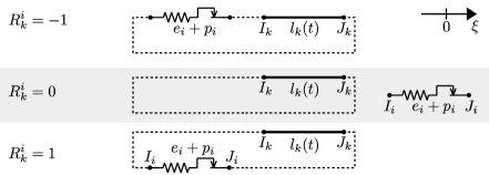
Figure 1: Illustration of the signs of the components of the incidence vector $R^{k}\in\mathbb{R}^{m}.$ The dotted contour stays for the chain of the springs associated with the vector $R^{k}$.

2.2 Stress-controlled loading

The stress-controlled loading $f_{i}$ models an external force applied at node $i,$ so that it affects the resultant of forces at node $i.$ We will study a so-called quasistatic evolution problem which further assumes that $f(t)$ can be balanced by the stresses of springs at any time. In other words, we assume that the stresses of springs, the reactions of displacement-controlled constraints, and the applied stress loading compensate one another at each of the $n$ nodes. In particular, for any $f(t)=const$ the system admits an equilibrium.

2.3 The variational system

With the notations introduced the quasistatic evolution of the stresses $s_{k}$ of springs and reactions $r_{k}$ of displacement-controlled loadings can be described by the following variational system (which corresponds to equations (6.1)-(6.6) in the abstract framework by Moreau moreau )

Elastic deformation: $$s=Ae,$$ (3)

Plastic deformation: $$\dot{p}\in N_{C}(s),$$ (4)

Geometric constraint: $$e+p\in D\mathbb{R}^{n},$$ (5)

Displacement-controlled loading: $$R^{\top}(e+p)=l(t),$$ (6)

Static balance under $$s_{k}s^{1}+\ldots+s_{m}s^{m}+$$

stress-controlled loading: $$+r_{1}r^{1}+\ldots+r_{q}r^{q}+f(t)=0,\hskip 28.45274pt$$ (7)

where

$$s=(s_{1},\ldots s_{m})^{\top} -$$ stresses of springs,

$$r=(r_{1},\ldots r_{q})^{\top} -$$ reactions of displacement-controlled loadings,

$$e=(e_{1},\ldots e_{m})^{\top} - \mbox{elastic elongations of springs},$$

$$p=(p_{1},\ldots p_{m})^{\top} -$$ plastic elongations of springs,

$$l(t)=\left(l_{1}(t),\ldots,l_{q}(t)\right)^{\top} - \mbox{enforced \hskip-1.13791ptlengths \hskip-1.13791ptbetween \hskip-1.13791ptnodes }\hskip-1.13791ptI_{i}\mbox{ \hskip-1.13791ptand }\hskip-1.13791ptJ_{i},\hskip-1.13791pt\ i\in\overline{1,q},$$

$$f(t)=\left(f_{1}(t),\ldots,f_{n}(t)\right)^{\top} -$$ stress-controlled loadings at nodes,

$$A={\rm diag}(a_{1},...,a_{m}) -$$ matrix of Hooke’s coefficients,

$$N_{C}(s)=\otimes_{i=1}^{m}N_{[c_{i}^{-},c_{i}^{+}]}(s) - \text{the normal cone to }C=\otimes_{i=1}^{m}[c_{i}^{-},c_{i}^{+}]\mbox{ at }s,$$

$$D\xi=\left(\xi_{j_{k}}-\xi_{i_{k}}\right)_{k=1}^{m} - \text{a linear map (represented by }m\times n\text{-matrix $D$)}$$

$$\text{that defines the graph of springs},$$

$$R=\left(R^{1},\ldots,R^{q}\right) - m\times q\mbox{-matrix of the incidence vectors},$$

$$\mbox{of displacement-controlled loadings}.$$

while the vectors $s^{k}=(s^{k}_{1},\ldots s^{k}_{n})^{\top}$ and $r^{k}=(r^{k}_{1},\ldots r^{k}_{n})^{\top}$ describe the signs of contributions of stresses of spring $k$ and reactions of displacement-controlled loading $k$ into the resultant of forces at nodes $1,...,n,$ i.e. (see Fig. 2)

• $s^{k}_{i}=-1,\ s^{k}_{i}=0,\ {\rm or}\ s^{k}_{i}=1,$ according to whether the spring $k$ is to the left from node $i,$ not connected to node $i,$ or is to the right from node $i,$

• $r^{k}_{i}=-1,\ r^{k}_{i}=0,\ {\rm or}\ r^{k}_{i}=1,$ according to whether the displacement-controlled loading $k$ is applied to the left from node $i,$ not applied to node $i,$ or applied to the right from node $i.$

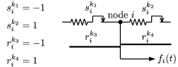
Figure 2: Examples of forces applied at node $i$.

The $m\times n$-matrix $D$ will be termed the kinematic matrix of the one-dimensional network of $m$ springs on $n$ nodes. Note, the matrix $-D^{\top}$ will then be the incidence matrix of the associated oriented graph of $n$ nodes and $m$ edges.

The static balance law (7) will further be written in the equivalent shorter form (31), which is similar to the one used by Moreau (moreau, , formula (3.23)). We believe, however, that formulation (7) creates a better idea as for why this law does indeed balance the forces.

Following Moreau moreau , we term system (3)-(7) an elastoplastic system.

3 Casting the variatonal system as a sweeping process

3.1 Derivation of the sweeping process

In order for (6) to be solvable in $e+p$ we assume that the displacement-controlled loadings $\{l_{i}(t)\}_{i=1}^{q}$ are independent in the sense that

$${\rm rank}\left(D^{\top}R\right)={\rm rank}\left(R^{\top}D\right)=q.$$ (8)

Mechanically, condition (8) ensures that the displacement-controlled loadings don’t contradict one another. For example, (8) rules out the situation where two displacement-controlled loadings connect same pair of nodes. It follows from condition (8) that the matrix equation

$$R^{\top}DL=I_{q\times q}.$$ (9)

has a $n\times q$ matrix solution. Furthermore, as we will show in the proof of Theorem 3.1, in order for equation (7) to be solvable in $s\in\mathbb{R}^{m}$ and $r\in\mathbb{R}^{q}$, the function $f(t)$ must satisfy $f(t)\in D^{\top}\mathbb{R}^{m}$. That is why, the existence of a continuous function $\bar{h}:\mathbb{R}\to\mathbb{R}^{m}$ such that

$$f(t)=-D^{\top}\bar{h}(t)$$ (10)

is our another assumption. As we further clarify in Remark 4, the proof of Theorem 3.1 implies that assumption (10) is equivalent to

$$f_{1}(t)+...+f_{n}(t)=0.$$ (11)

Introducing

$$U=\left\{x\in D\mathbb{R}^{n}:R^{\top}x=0\right\},\qquad V=A^{-1}U^{\perp},$$ (12)

where

$$U^{\perp}=\left\{y\in\mathbb{R}^{m}:\left<x,y\right>=0,\ x\in U\right\},$$ (13)

the space $V$ will be the orthogonal complement of the space $U$ in the sense of the scalar product

$$(u,v)_{A}=\left<u,Av\right>.$$ (14)

Therefore, any element $x\in\mathbb{R}^{m}$ can be uniquely decomposed as

$$x=P_{U}x+P_{V}x,$$

where $P_{U}$ and $P_{V}$ are linear (orthogonal in sense of (14)) projection maps on $U$ and $V$ respectively. Define

$$g(t) =P_{V}DLl(t),$$ (15)

$$h(t) =P_{U}A^{-1}\bar{h}(t),$$ (16)

$$N_{C}^{A}(x) =\left\{\begin{array}[]{ll}\left\{\xi\in\mathbb{R}^{m}:\left<\xi,A(c-x)\right>\leq 0,\ {\rm for\ any}\ c\in C\right\},&\quad{\rm if}\ x\in C,\\ \emptyset,&\quad{\rm if}\ x\not\in C,\end{array}\right.$$ (19)

$$\Pi(t) =A^{-1}C+h(t)-g(t),$$ (20)

and consider the following differential inclusions

$$-\dot{y} \in N^{A}_{\Pi(t)\cap V}(y),$$ (21)

$$\dot{z} \in\left(N^{A}_{\Pi(t)}(y)+\dot{y}\right)\cap U,$$ (22)

with initial conditions

$$y(0) \in\Pi(0)\cap V,$$ (23)

$$z(0) \in U.$$ (24)

The function $g(t)$ will be termed the effective displacement-controlled loading. Similarly, $h(t)$ is termed the effective stress loading.

In what follows we are going to establish an equivalence between systems (3)-(7) and (21)-(24).

According to Moreau (moreau, , Proposition of §6.d), the problem (22), (24) admits an absolutely continuous (possibly non-unique) solution $z$ on $[0,T]$ for any absolutely continuous solution $y$ of (21), (23) defined on $[0,T]$. The analysis of the dynamics of the elastic deformation $e(t)$ therefore reduces to the analysis of the solution $y$ of the sweeping process (21). In particular, stabilization of (21) will imply stabilization of both elastic deformations $e(t)=(e_{1}(t),...,e_{m}(t))^{\top}$ and stresses $s(t)=(s_{1}(t),...,s_{m}(t))^{\top}$ of springs.

Theorem 3.1

Let $D$ be the kinematic matrix of a connected network of $m$ elastoplastic springs on $n$ nodes. Let $R$ be a matrix of incidence vectors of $q$ displacement-controlled constraints, which are independent in the sense of (8). Assume that the stress loading doesn’t exceed the safe load bounds, i.e.

$$\left(C+Ah(t)\right)\cap U^{\perp}\not=\emptyset,\ {for\ all\ }t\in[0,T],$$ (25)

holds for $C$, $U$ and $h$ as defined in (4), (12), and (16). If $(s(t),e(t),p(t),r(t))$ is a solution of the variational system (3)-(7) on $[0,T],$ then

$$\begin{array}[]{l}y(t)=e(t)+h(t)-g(t),\\ z(t)=e(t)+p(t)+h(t)-g(t)\end{array}$$ (26)

is a solution of the sweeping process (21)-(24) on $[0,T].$ Conversely, if $(y(t),z(t))$ is a solution of (21)-(24) then $(e(t),p(t))$ found from (26) is a solution of (3)-(7) with $s(t)=Ae(t)$ and with some suitable $r(t).$

We refer the reader to Had-Reddy han for formulations of the safe load condition (25) in the context of classical (continuum) theory of plasticity.

Remark 1

Since $P_{U}g(t)=0$, condition (25) is equivalent to assuming $\Pi(t)\cap V\not=\emptyset,$ $t\in[0,T].$

Remark 2

Condition (25) always holds when $h(t)\equiv 0$ because $0\in C$ and $0\in U^{\perp}$. Geometrically, condition (25) means that the parallelepiped $\Pi(t)$ and the hyperplane $V$ in Fig. 3 do intersect. Mechanically, condition (25) accounts for the fact that the stresses of the elastoplastic springs are bounded and cannot balance arbitrary large stress loadings.

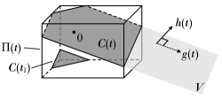
Figure 3: Moving constraint for different values of time. a

Remark 3

The function $g(t)$ and the matrix $P_{V}DL$ don’t depend on the choice of matrix $L$. Indeed, let $\tilde{g}(t)$ be the function $g(t)$ obtained by replacing $L$ by $\tilde{L}$. Then using (12) we get

$$0_{q\times q}=R^{\top}D(L-\tilde{L})=R^{\top}(P_{U}D(L-\tilde{L})+P_{V}D(L-\tilde{L}))=R^{\top}P_{V}D(L-\tilde{L}),$$

so $P_{V}D(L-\tilde{L})\mathbb{R}^{q}\subset U$. Therefore, $P_{V}D(L-\tilde{L})=0_{m\times m}$ and $P_{V}DL=P_{V}D\tilde{L}$. The conclusion about $g(t)$ follows from (15).

In Appendix B we offer a diagram (fig. 7) showing graphically how the spaces $U,V$ and the moving set $\Pi(t)\cap V$ are constructed.

Proof of Theorem 3.1. The system of (5) and (6) is equivalent to

$$e(t)+p(t)\in U^{l}(t),\quad{\rm where}\quad U^{l}(t)=\left\{x\in D\mathbb{R}^{n}:R^{\top}x=l(t)\right\}.$$ (27)

Applying the both sides of (9) to $l(t)$, we get $R^{\top}DLl(t)=l(t)$, which implies $DLl(t)\in U^{l}(t).$ Therefore,

$$U^{l}(t)=U+DLl(t)$$

and (27) can be rewritten as

$$e(t)+p(t)\in U+DLl(t),$$

or, equivalently,

$$e+p\in U+g(t).$$ (28)

By the definition of matrix $D$, the $i$-th line has $+1$ ($-1$) at those nodes which are right (left) endpoints for the $j$-th spring, see the illustration at fig. 4. Therefore,

$$s_{1}s^{1}+\ldots+s_{m}s^{m}=-D^{\top}s.$$ (29)

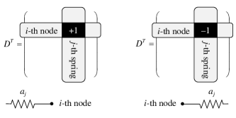
Figure 4: The meaning of the columns and rows of matrix $D^{\top}.$ The cell equals $+1$, if the $i$-th node is the right endpoint for spring $j$. Conversely, the cell equals $-1$, if the $i$-th node is the left endpoint for spring $j$.

Now we are going to demonstrate that it is enough to use the description of displacement-controlled loadings $R^{k}$(which is it terms of springs lengths), i.e

$$r_{1}r^{1}+\ldots+r_{q}r^{q}=-D^{\top}Rr,\qquad{\rm where}\quad r=\left(r_{1},\ldots,r_{q}\right)^{\top}.$$ (30)

Indeed, by Fig. 4, the matrix $\left(\begin{array}[]{c}-D\\ (r^{k})^{\top}\end{array}\right)^{\top}$ is the incidence matrix of the oriented graph of springs $s_{1},...,s_{m}$ on nodes $1,...,n$ supplemented with a virtual spring connecting the nodes $\xi_{I_{k}}<\xi_{J_{k}}$ (see section 2.1 earlier). We can now use this virtual spring in order to close the chain of springs given by the incidence vector $R^{k}$ and obtain a directed cycle where the direction from the node $I_{k}$ to the node $J_{k}$ disagree with the direction of the virtual spring. The incidence vector of this cycle is $\left(\begin{array}[]{c}R^{k}\\ -1\end{array}\right).$ According to (bapat, , p. 57), we now have

$$\left(\begin{array}[]{c}-D\\ (r^{k})^{\top}\end{array}\right)^{\top}\left(\begin{array}[]{c}R^{k}\\ -1\end{array}\right)=0,\qquad k\in\overline{1,q},$$

from which (30) follows.

Therefore, taking into account (29), one concludes that (7) can be rewritten as

$$-D^{\top}s-D^{\top}Rr+f(t)=0,$$ (31)

which has a solution $(s(t),r(t))$ if and only if

$$s(t)+Rr(t)+\bar{h}(t)\in{\rm Ker}~{}D^{\top}.$$

Keeping $s(t)$ fixed, the latter inclusion can be solved for $r(t)\in\mathbb{R}^{q}$ if and only if

$$s(t)+\bar{h}(t)\in{\rm Ker}~{}D^{\top}+R\,\mathbb{R}^{q}=\left(D\mathbb{R}^{n}\right)^{\perp}+\left\{x\in\mathbb{R}^{m}:R^{\top}x=0\right\}^{\perp}=\\ =\left(D\mathbb{R}^{n}\cap\left\{x\in\mathbb{R}^{m}:R^{\top}x=0\right\}\right)^{\perp}=U^{\perp},$$ (32)

see e.g. Friedberg et al (algebrabook, , Exercise 17, p. 367) for the property ${\rm Ker}~{}D^{\top}=\left(D\mathbb{R}^{n}\right)^{\perp}$. If $s(t)$ satisfies (32), then by (16)

$$\begin{array}[]{r}s(t)+Ah(t)=s+A\left(P_{U}A^{-1}\bar{h}(t)+P_{V}A^{-1}\bar{h}(t)-P_{V}A^{-1}\bar{h}(t)\right)\in\\ \in s+AA^{-1}\bar{h}(t)+AV=s+\bar{h}(t)+U^{\perp}\in U^{\perp}.\end{array}$$ (33)

Vice versa, if $s(t)$ satisfies (33) then

$$\begin{array}[]{r}s(t)+\bar{h}(t)=s+A\left(P_{U}A^{-1}\bar{h}(t)+P_{V}A^{-1}\bar{h}(t)\right)=\\ =s(t)+Ah(t)+AP_{V}A^{-1}\bar{h}(t)\in U^{\perp},\end{array}$$

which is (32). By applying $A^{-1}$ to (33), we get

$$e+h(t)\in V.$$ (34)

Since $g(t)\in V$ and $h(t)\in U$ we can rewrite (28), (34) and (4) as

$$e+p-g(t)+h(t) \in U,$$

$$e+h(t)-g(t) \in V,$$

$$\dot{p} \in N_{C}(Ae).$$

Introducing the change of the variables (26) we have $p=z-y$ and using the substitution $e=y-h(t)+g(t)$

$$\begin{array}[]{l}\dot{z}-\dot{y}\in N^{A}_{A^{-1}C}(y-h(t)+g(t)),\\ z\in U,\\ y\in V.\end{array}$$ (35)

Let $(y,z)$ be a solution of (35). Since $z\in U$ we have $-\dot{z}\in-U=U=V^{\perp_{A}}=N^{A}_{V}(y)$, where $V^{\perp_{A}}$ is the orthogonal complement of $V$ in the sense of the scalar product $(\cdot,\cdot)_{A},$ and the inclusion (21) computes as follows:

$$\begin{array}[]{r}-\dot{y}\in N^{A}_{A^{-1}C}(y-h(t)+g(t))-\dot{z}\in N^{A}_{A^{-1}C+h(t)-g(t)}(y)+N^{A}_{V}(y)=\\ =N^{A}_{(A^{-1}C+h(t)-g(t))\cap V}(y),\end{array}$$

where the last equality holds due to (25) (where both intersecting sets are polyhedral, we use (Rockafellar, , Corollary 23.8.1)). The inclusion (22) follows by combining

$$\dot{z}=\dot{z}-\dot{y}+\dot{y}\in N^{A}_{A^{-1}C+h(t)-g(t)}(y)+\dot{y},$$

with the property $z(t)\in U$ observed in (35). Vice versa, if $(y,z)$ is a solution of (21)-(22), then

$$-y\in V,$$

$$\dot{z}\in N^{A}_{A^{-1}C+h(t)-g(t)}(y)+\dot{y},$$

$$\dot{z}\in U,$$

which implies (35) when combined with (24). ∎

Remark 4

Having the proof of Theorem 3.1 behind, we can now clarify why the $n$ equations (7) of static balance in nodes is equivalent to just one equation (11). Indeed, as it follows from the proof of Theorem 3.1, equation (7) is equivalent to (31) which necessarily means that

$$f(t)\in D^{\top}\mathbb{R}^{m}.$$ (36)

It remains to show that (36) is equivalent to (11). Since ${\rm dim\,Ker}\,D+{\rm rank}\,D=n$, by rank-nullity theorem (see e.g. (algebrabook, , Theorem 2.3)) and ${\rm rank}\,D=n-1$ by Bapat (bapat, , Lemma 2.2) (the rank of the incidence matrix of a connected graph is one less the number of nodes), one has $\dim{\rm Ker}\,D=1.$ On the other hand, $D(1,...,1)^{\top}=0$ by inspection. Therefore, $D^{\top}\mathbb{R}^{m}=({\rm Ker}\hskip 1.42271ptD)^{\perp}=\left\{x:(1,...,1)x=0\right\},$ i.e. (36) is equivalent to (11).

We acknowledge that the ideas of the proof of Theorem 3.1 are due to Moreau moreau , who however worked in abstract configuration spaces and didn’t give details that relate the sweeping process (21) to networks of connected springs (3)-(7).

Formulas (15)-(20) establish a connection between mechanical properties of applied loading and geometric properties of the moving constraint $\Pi(t)\cap V$. Specifically, varying the stress loading $f(t)$ moves $\Pi(t)$ in the direction perpendicular to $V$ in the sense of the scalar product (14). In contrast, varying the displacement-controlled loading $l(t)$ moves $\Pi(t)$ in the direction parallel $V.$ We also see that the variety of possible perpendicular motions coming from $f(t)$ is limited by the dimension of the space $U,$ which will be computed in section 3.2 (Lemma 1). The dimension of possible directions for the parallel motion in $V$ is not always $\dim V,$ but is related to the rank of matrix $\bar{L}$, which we compute in section 3.4, see formula (51).

3.2 Sweeping processes of particular elastoplastic systems

In this section we consider particular networks of elastoplastic springs and offer a guideline that can be used to derive the associated sweeping process (21) in closed form.

The following lemma will be used to compute the dimension of $U.$

Lemma 1

If (8) is satisfied, then

$$\dim U=n-q-1.$$ (37)

Proof. Let $E=D\mathbb{R}^{n}.$ Viewing $R^{\top}$ as a linear map from $E$ to $\mathbb{R}^{q}$ the rank-nullity theorem (see e.g. Friedberg et al (algebrabook, , Theorem 2.3)) gives

$${\rm dim\,Ker}\,R^{\top}+{\rm rank}\hskip 1.42271ptR^{\top}=\dim E,$$

where ${\rm dim\,Ker}\,R^{\top}=\dim U$ by (12), ${\rm rank}\,R^{\top}=q$ by (8), and $\dim E=n-1$ by Bapat (bapat, , Lemma 2.2). ∎

Example. Consider a one-dimensional network of 3 springs on 4 nodes with the kinematic matrix $D$ provided by the map

$$D\xi=\begin{pmatrix}\xi_{2}-\xi_{1}\\ \xi_{3}-\xi_{2}\\ \xi_{4}-\xi_{3}\end{pmatrix}=\begin{pmatrix}-1&1&0&0\\ 0&-1&1&0\\ 0&0&-1&1\end{pmatrix}\begin{pmatrix}\xi_{1}\\ \xi_{2}\\ \xi_{3}\\ \xi_{4}\end{pmatrix},$$ (38)

some $3\times 3$ diagonal matrix $A$ of Hooke’s coefficients and some intervals $[c_{i}^{-},c_{i}^{+}]$, $i\in\overline{1,3}$, of elasticity bounds. Assume that displacement-controlled loading $l(t)\in\mathbb{R}^{2}$ is given by the incidence vectors

$$(R_{1},R_{2})=R=\left(\begin{array}[]{ll}0&1\\ 1&1\\ 1&0\end{array}\right),$$ (39)

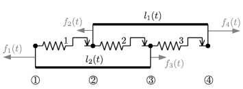
Figure 5: A one-dimensional network of 3 springs on 2 nodes with 2 length locking constraints. The circled figures stays for numbers of nodes. The regular figures are the numbers of springs. The figure shows just one possible option for the directions (and magnitudes) of the forces in gray color.

see Fig. 5. To examine the shapes of the associated moving set $\Pi(t)\cap V$, we find out the eligible values of the function $h(t)$.

From (16) we conclude that eligible stress-controlled loading $f(t)$ lead to $h(t)$ given by

$$h(t)=U_{basis}H(t),$$ (40)

where $~{}U_{basis}$ is the $m\times{\dim U}-$matrix of the vectors of a basis of $U$ and $H:[0,T]~{}\to\mathbb{R}^{\dim U}$ is any absolutely continuous function.By (37) and (12), there should exist an $n\times(n-q-1)-$matrix $M$ such that

$$R^{\top}DM=0\quad{\rm and}\quad{\rm rank}(DM)=n-q-1$$ (41)

which allows to introduce $U_{basis}$ as

$$U_{basis}=DM.$$ (42)

Getting back to the matrices $D$ and $R$ given by (38) and (39) one has $\dim U=n-q-1=4-2-1=1$. A possible $4\times 1-$matrix that solves (41), the respective $U_{basis}$ found from (42), and the respective function $h(t)$ given by (40) are then read as

$$M=\left(\begin{array}[]{c}0\\ 1\\ 0\\ 1\end{array}\right),\quad U_{basis}=\left(\begin{array}[]{c}1\\ -1\\ 1\end{array}\right),\quad h(t)=\left(\begin{array}[]{c}1\\ -1\\ 1\end{array}\right)H(t),$$ (43)

where $H$ is an arbitrary absolutely continuous function from $[0,T]$ to $\mathbb{R}.$ Fig. 6 illustrates the shapes of $\Pi(t)\cap V$ for different constant values of $H(t),$ where according to (12) we considered

$$V={\rm Ker}\,\left(U_{basis}^{\top}A\right)=\left(\begin{array}[]{c}a_{1}\\ -a_{2}\\ a_{3}\end{array}\right)^{\perp}.$$ (44)

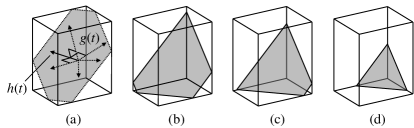
Figure 6: Shapes of the moving constraint $\Pi(t)\cap V$ for the sweeping process of the network of Fig. 5 with parameters $c_{1}^{+}=-c_{1}^{-}=1,c_{2}^{+}=-c_{2}^{-}=1.3,c_{3}^{+}=-c_{3}^{-}=1.6,a_{1}=a_{2}=a_{3}=1$ for different values of stress loading $h(t)=(1,-1,1)^{\top}t$:                                            a) $t=0$, b) $t=0.32,$ c) $t=0.5$, d) $t=0.8$. Figure (a) also features the possible directions of the function $g(t)$ (dotted vectors) and the possible direction of the function $h(t)$ (solid vector) that represent displacement-controlled and stress-controlled loading respectively.

3.3 Bounds on the stress loading to satisfy the safe load condition

In this section we are dealing with a general elastoplastic system again. To verify condition (8) it is sufficient to check that displacement-controlled lengths $l_{i}(t)$ can be varied independently one from another. Computational algorithms to verify safe load condition (25) for particular systems is a standard topic of computational geometry, see e.g. Bremner et al bremner . In this section we derive analytic conditions which allow to spot classes of elastoplastic systems for which the safe load condition holds.

Proposition 1

In order for the safe load condition (25) of Theorem 4.1 to hold for some $t\geq 0,$ it is sufficient to assume that

$$-Ah(t)\in C.$$ (45)

Proof. In order to show that (45) implies (25), it is sufficient to observe that $0\in U^{\perp}$ and that (45) yields $0\in C+Ah(t)$.∎

Definition 1

We will say that a spring $i$ is blocked by displacement-controlled loadings, if the family of displacement-controlled loadings $\{l_{j}\}_{j=1}^{q}$ contains a chain that connects one end of spring $i$ with its other end.

Lemma 2

Assume that in a given elastoplastic system the number $q$ of displacement-controlled loadings is 2 less the number of nodes. If none of the springs of the elastoplastic system (3)-(7) is blocked by displacement-controlled loadings, then

$$x_{i}\not=0\mbox{ for any }i\in\overline{1,m},\ x\in U\backslash\{0\}.$$

Proof. Recall, that $I_{k}$ and $J_{k}$ are the left and right endpoints respectively of the displacement-controlled constraint $l_{k}(t).$ Consider the matrix $D_{1}$ obtained from matrix $D$ by combining the column $I_{k}$ and the column $J_{k}$ as follows: 1) add the values of column $J_{k}$ to the respective values of column $I_{k}$, 2) delete the column $J_{k}.$ Then,

$$\left\{D_{1}\xi:\xi\in\mathbb{R}^{n-1}\right\}=\left\{D\xi:(R^{k})^{\top}D\xi=0,\ \xi\in\mathbb{R}^{n}\right\}.$$

Moreover, each row of $D$ has exactly one element $1$ and $-1$ and none of the springs are blocked therefore at least one of each pair of summands at step 1) is zero. Matrix $D_{1}$ is the kinematic matrix for a new elastoplastic system that is obtained from elastoplastic system (3)-(7) by merging the nodes $I_{k}$ and $J_{k}$ together and, thus, by reducing the number of nodes by 1. Accordingly, the new elastoplastic system features only $q-1$ displacement-controlled loadings and the indices $\{I_{i},J_{i}\}_{i=1}^{q-1}$ are now from $\overline{1,n-1}.$

Repeating this process through all the incidence vectors $\{R^{k}\}_{k=1}^{q},$ where $q=n-2$ by Lemma 1, we obtain

$$U=\left\{D\xi:R^{\top}D\xi=0,\ \xi\in\mathbb{R}^{n}\right\}=\left\{\bar{D}\xi:\xi\in\mathbb{R}^{n-q}\right\}=\left\{\bar{D}\xi:\xi\in\mathbb{R}^{2}\right\},$$

where $\bar{D}$ is the kinematic matrix of the reduced elastoplastic system that is obtained from the original one by merging node $I_{k}$ with node $J_{k}$ trough $k\in\overline{1,q}.$

Since the reduced elastoplastic system has only two nodes ($q=n-2$), all the displacement-controlled constraints of the original system split into at most two connected components, which shrink into these two nodes under the proposed reduction process. If spring $i$ is not blocked by displacement-controlled loadings, then the endpoints of spring $i$ belong to different connected components introduced. Therefore, the endpoints of spring $i$ are two different nodes of the reduced elastoplastic system, which implies

$$u_{i}\not=0,\ i\in\overline{1,m},\quad\mbox{for any }u=\bar{D}\xi\ \text{such that }\xi\in\mathbb{R}^{2},\xi_{1}\neq\xi_{2}.$$

If $\xi_{1}=\xi_{2}$ then $u=\bar{D}\xi=0$. The proof of the lemma is complete.∎

Proposition 2

Assume that the conditions of Lemma 2 hold. Let $\bar{u}$ be an arbitrary nonzero fixed vector of $U$ ($\dim U=1$ by Lemma 1) and consider

$$\bar{c}^{+}=\left(\begin{array}[]{c}c_{1}^{{\rm\hskip 0.5ptsign\hskip 1.0pt}(\bar{u}_{1})}\\ \vdots\\ c_{m}^{{\rm\hskip 0.5ptsign\hskip 1.0pt}(\bar{u}_{m})}\end{array}\right),\qquad\bar{c}^{-}=\left(\begin{array}[]{c}c_{1}^{-{\rm\hskip 0.5ptsign\hskip 1.0pt}(\bar{u}_{1})}\\ \vdots\\ c_{m}^{-{\rm\hskip 0.5ptsign\hskip 1.0pt}(\bar{u}_{m})}\end{array}\right),$$

where $c_{i}^{-1}$ denotes $c_{i}^{-}$ and $c_{i}^{+1}$ denotes $c_{i}^{+}$. Then, for each fixed $t\geq 0,$ the safe load condition (25) holds if and only if

$$\left<\bar{u},\bar{c}^{+}+Ah(t)\right>\cdot\left<\bar{u},\bar{c}^{-}+Ah(t)\right>\leq 0.$$ (46)

Proof. We first show that (46) implies (25). Assume that (25) doesn’t hold for some $t\in[0,T].$ Therefore, by convexity of $C$, either $\left<\bar{u},x+Ah(t)\right>>0$ for all $x\in C$ or $\left<\bar{u},x+Ah(t)\right><0$ for all $x\in C$. In either case we conclude $\left<\bar{u},\bar{c}^{+}+Ah(t)\right>\cdot\left<\bar{u},\bar{c}^{-}+Ah(t)\right>>0$ because $\bar{c}^{+},\bar{c}^{-}\in C,$ which contradicts (46).

Let us now show that (25) implies (46). Indeed, since

$$\bar{u}_{i}\bar{c}_{i}^{-}\leq\bar{u}_{i}c_{i}^{j}\leq\bar{u}_{i}\bar{c}_{i}^{+},\quad\mbox{for any }i\in\overline{1,m},\ j\in\{-1,+1\},$$

we have

$$\left<\bar{u},\bar{c}^{-}+Ah(t)\right>\leq\left<\bar{u},x+Ah(t)\right>\leq\left<\bar{u},\bar{c}^{+}+Ah(t)\right>,\quad\mbox{for any }x\in C.$$

The latter inequality takes the required form (46) when one plugs $x$ satisfying $\left<\bar{u},x+Ah(t)\right>=0$, which exists because of (25).∎

Remark 5

Considering the left-hand-side of (46) as a polynomial $P\left(\left<\bar{u},Ah(t)\right>\right)$ in $\left<\bar{u},Ah(t)\right>$, we see that the branches of the polynomial are pointing upwards. Therefore, condition (46) is the requirement for $\left<\bar{u},Ah(t)\right>$ to stay strictly between the roots of the polynomial. The roots of $P\left(\left<\bar{u},Ah(t)\right>\right)$ are given by $\left<\bar{u},Ah(t)\right>=-\left<\bar{u},\bar{c}^{-}\right>>0$ and $\left<\bar{u},Ah(t)\right>=-\left<\bar{u},\bar{c}^{+}\right><0$. Therefore, (46) is equivalent to

$$-\left<\bar{u},\bar{c}^{+}\right>\leq\left<\bar{u},Ah(t)\right>\leq-\left<\bar{u},\bar{c}^{-}\right>,$$

which highlights that (46) is a restriction on the magnitude of $\left<\bar{u},Ah(t)\right>.$

Proposition 2 can be e.g. applied to the one-dimensional network of Fig. 5, where $\dim U=1$ as we noticed earlier.

Example (continued). For the elastoplastic system of Fig. 5 one can consider $\bar{u}=(1,-1,1)^{\top}$ and using (43) obtain

$$\bar{c}^{+}=\left(\begin{array}[]{c}c_{1}^{+}\\ c_{2}^{-}\\ c_{3}^{+}\end{array}\right),\quad\bar{c}^{-}=\left(\begin{array}[]{c}c_{1}^{-}\\ c_{2}^{+}\\ c_{3}^{-}\end{array}\right),\quad\left<\bar{u},Ah(t)\right>=(a_{1}+a_{2}+a_{3})H(t).$$ (47)

Based on Remark 5 the necessary and sufficient condition for safe load condition (46) to hold is then

$$-c_{1}^{+}+c_{2}^{-}-c_{3}^{+}\leq(a_{1}+a_{2}+a_{3})H(t)\leq-c_{1}^{-}+c_{2}^{+}-c_{3}^{-}.$$ (48)

3.4 Condition on the displacement-controlled loading to eliminate constant solutions

Next proposition gives conditions to ensure that any point $x$ which belongs to the moving set $\Pi(t)\cap V$ of sweeping process (21) at some initial time $t=t_{1}$ will lie outside $\Pi(t)\cap V$ at time $t=t_{2}.$ These conditions will, therefore, rule out the existence of constant solutions.

Proposition 3

Assume that conditions of Theorem 3.1 hold. If

$$\|A^{-1}c^{-}-A^{-1}c^{+}\|_{A}<\left\|g(t_{1})-g(t_{2})\right\|_{A},$$ (49)

for some $0\leq t_{1}<t_{2}$, where

$$\|x\|_{A}=\sqrt{\left<x,Ax\right>},\quad c^{-}=(c_{1}^{-},...,c_{m}^{-})^{\top},\quad c^{+}=(c_{1}^{+},...,c_{m}^{+})^{\top},$$

then sweeping process (21) doesn’t have any solutions that are constant on $[t_{1},t_{2}].$

Proof. The claim follows by showing that

$$\left(\Pi(t_{1})\cap V\right)\cap\left(\Pi(t_{2})\cap V\right)=\emptyset$$

Since $h(t)\in U$ we have

$$\Pi(t)\cup V=\left(A^{-1}C+h(t)-g(t)\right)\cap V\subset P_{V}A^{-1}C-g(t),\quad t\in[t_{1},t_{2}],$$

and it is sufficient to prove that the sets

$$P_{V}A^{-1}C-g(t_{1})\ \ {\rm and}\ \ P_{V}A^{-1}C-g(t_{2})\ \ \mbox{don't intersect}.$$

The latter will hold, if the diameter of the set $P_{V}A^{-1}C$ is smaller than the distance between $g(t_{1})$ and $g(t_{2}),$ which fact will now be established.

Since $P_{V}$ is the orthogonal projection in the sense of the scalar product $(x,y)_{A}=\left<x,Ay\right>,$ we have (see e.g. Conway (conway, , Theorem 2.7 b)))

$$\|P_{V}x\|_{A}\leq\|x\|_{A},\quad x\in\mathbb{R}^{m}.$$

Therefore, for any $c_{1},c_{2}\in C$,

$$\left\|P_{V}\left(A^{-1}c_{1}-A^{-1}c_{2}\right)\right\|_{A}\leq\left\|A^{-1}c_{1}-A^{-1}c_{2}\right\|_{A}\leq\|A^{-1}c^{-}-A^{-1}c^{+}\|_{A}<$$

$$<\left\|g(t_{1})-g(t_{2})\right\|_{A}.$$

The proof of the proposition is complete.

Remark 6

Note, the left-hand-side in the squared inequality (49) from the statement of Proposition 3 can be computed as
$\|A^{-1}c^{-}-A^{-1}c^{+}\|_{A}^{2}=\left<c^{-}-c^{+},A^{-1}(c^{-}-c^{+})\right>.$

In what follows we show which kind of computations is required to verify the condition of Proposition 3 in practice.

Example (continued). Given the elastoplastic system of Fig. 5, our goal is to compute the effective displacement-controlled loading $g(t)$ of (15).

For the term $P_{V}DL$ of (15) observe, that there exists a $\dim V\times q$-matrix $\bar{L}$ such that

$$V_{basis}\bar{L}=P_{V}DL,$$ (50)

where $V_{basis}$ is the $m\times\dim V-$matrix of the vectors of a basis of $V$. The $i$-th column of matrix $\bar{L}$ is the vector of the coordinates of the respective vector $P_{V}DL^{i}\in V$ in the basis $V_{basis},$ where $L^{i}$ stays for the $i$-th column on matrix $L.$ Formula (15) can therefore be rewritten as

$$g(t)=V_{basis}\bar{L}l(t).$$ (51)

Computing the effective displacement-controlled loading $g(t)$ has hereby been turned into computing $V_{basis}$ and $\bar{L}$.

By (37),

$$\dim V=m-n+q+1,$$ (52)

and according to (44), $V_{basis}$ is an arbitrary matrix of $\dim V$ linearly independent columns that solves

$$(U_{basis})^{\top}AV_{basis}=0.$$ (53)

For the particular matrices (38), using the earlier computed $U_{basis}$, see (43), one gets $\dim V=2$, $(U_{basis})^{\top}=(1\ -1\ 1)$, and a possible solution to (53) is

$$V_{basis}=\left(\begin{array}[]{cc}1/a_{1}&0\\ 1/a_{2}&1/a_{2}\\ 0&1/a_{3}\end{array}\right).$$

To find $\bar{L}$, we observe that by (9), for any $\xi\in\mathbb{R}^{q}$, we have

$$P_{V}DL\xi=DL\xi-P_{U}DL\xi\in D\mathbb{R}^{n},$$

as $P_{U}DL\xi\in D\mathbb{R}^{n}$ by definition of $U.$ Combining this relation with (9) and (50) one gets the following equations for $\bar{L}$:

$$R^{\top}V_{basis}\bar{L} =I_{q\times q},$$ (54)

$$V_{basis}\bar{L}\,\mathbb{R}^{q} \subset D\mathbb{R}^{n},$$ (55)

from which $\bar{L}$ can be found. In Appendix B we offer a diagram (fig. 7) showing the construction of $V_{basis}\bar{L}$ graphically.

For specific matrix $D$ given by (38), one has $D\mathbb{R}^{4}=\mathbb{R}^{3}$ (i.e. there is no geometric constraint coming from the graph of springs in this case) and so (55) holds for any matrix $\bar{L}.$ The matrix $\bar{L}$ is therefore a $2\times 2-$matrix that solves (54), which has a unique solution

$$\bar{L}=\left(\begin{array}[]{cc}1/a_{2}&1/a_{2}+1/a_{3}\\ 1/a_{1}+1/a_{2}&1/a_{2}\end{array}\right)^{-1}.$$

Formula (51), in particular, implies that, for the network of springs of Fig. 5 (where $\dim V=q=2$), the displacement-controlled constraints are capable to execute any desired motion of $C(t)$ in $V.$

Applying Proposition 3 and Remark 6, we obtain the following condition for non-existence of constant solutions. The elastoplastic system of Fig. 5 doesn’t have constant solutions on $[0,T]$, if there exist $t_{1},t_{2}\in[0,T]$ such that

$$\sum_{i=1}^{4}\dfrac{1}{a_{i}}(c_{i}^{+}-c_{i}^{-})^{2}<\left\|V_{basis}\bar{L}\left(l(t_{1})-l(t_{2})\right)\right\|^{2}_{A}.$$ (56)

3.5 A polyhedral description of moving sets for elastoplastic systems and reduction to subspace $V$

To give a deeper look into the possible dynamics of sweeping processes of elastoplastic systems we now rewrite moving set $\Pi(t)\cap V$ and process (22) in a slightly different form which is more suitable for further analysis. From

$$A^{-1}C=\left\{x\in\mathbb{R}^{m}:\dfrac{1}{a_{i}}c_{i}^{-}\leq x_{i}\leq\dfrac{1}{a_{i}}c_{i}^{+}\right\}$$

we have

$$A^{-1}C+h(t)-g(t)=\left\{x\in\mathbb{R}^{m}:c_{i}^{-}+a_{i}h_{i}(t)\leq\left<e_{i},Ax+Ag(t)\right>\leq c_{i}^{+}+a_{i}h_{i}(t)\right\},$$

where $e_{i}\in\mathbb{R}^{m}$ is the vector with 1 in the $i$-th component and zeros elsewhere. Since $g(t)\in V,$ one has

$$\left<e_{i},Ax+Ag(t)\right>=\left<P_{U}e_{i}+P_{V}e_{i},Ax+Ag(t)\right>=\left<P_{V}e_{i},Ax+Ag(t)\right>,\quad x\in V,$$

and we conclude

$$\Pi(t)\cap V=\bigcap_{i=1}^{m}\left\{x\in V:c_{i}^{-}\hskip-1.42271pt+\hskip-1.42271pta_{i}h_{i}(t)\hskip-1.42271pt\leq\hskip-1.42271pt\left<n_{i},Ax\hskip-1.42271pt+\hskip-1.42271ptAg(t)\right>\hskip-1.42271pt\leq\hskip-1.42271ptc_{i}^{+}\hskip-1.42271pt+\hskip-1.42271pta_{i}h_{i}(t)\right\},$$ (57)

where $n_{i}=P_{V}e_{i}$, i.e. $n_{i}$ are the columns of the projection matrix $P_{V}$.

Moreover, since $y(t)\in V$ for all $t$ and $y^{\prime}(t)\in V$ for a.a. $t$ we can restrict the normal cone from (22) to the normal cone defined within the subspace $V$, which also appears to be the intersection of the original normal cone with $V$:

$$N^{V}_{\mathcal{C}}(x):=N^{A}_{\mathcal{C}}(x)\cap V=\left\{\begin{array}[]{ll}\left\{\xi\in V:\left<\xi,A(c-x)\right>\leq 0,\ {\rm for\ any}\ c\in\mathcal{C}\right\},&\text{ if }x\in\mathcal{C},\\ \emptyset,&\text{ if }x\not\in\mathcal{C}.\end{array}\right.$$

Therefore we can restrict sweeping process (22) to one completely defined within $V$:

$$-\dot{y}\in N^{V}_{\Pi(t)\cap V}(y).$$ (58)

In the following chapters we are going to analyze dynamics of the process (58) with the moving set in form (57).

4 Convergence to a periodic attractor

4.1 Convergence in the case of a moving constraint given by an intersection of translationally moving convex sets

In this section we establish convergence properties of a general sweeping process

$$-\dot{x}\in N_{C(t)}^{0}(x),\qquad y\in E,$$ (59)

where $E$ is a $d$-dimensional linear vector space, $C(t)\subset E$ is convex closed set for any $t$, and

$$N_{C}^{0}(x)=\left\{\begin{array}[]{ll}\left\{\xi\in E:\left(\xi,c-x\right)_{0}\leq 0,\ {\rm for\ any}\ c\in C\right\},&\quad{\rm if}\ x\in C,\\ \emptyset,&\quad{\rm if}\ x\not\in C,\end{array}\right.$$ (60)

where $(\cdot,\cdot)_{0}$ is some inner product in $E.$ These convergence properties are then refined in section 4.3 in the context of the particular sweeping process (21).

A set-valued function $t\mapsto C(t)$ is called globally Lipschitz continuous, if

$$d_{H}(C(t_{1}),C(t_{2}))\leq L_{C}|t_{1}-t_{2}|,\ \mbox{for all}\ t_{1},t_{2}\in\mathbb{R},\mbox{ and for some }L_{C}>0,$$ (61)

where $d_{H}(C_{1},C_{2})$ is the Hausdorff distance between two closed sets $C_{1},C_{2}\in E$ defined as

$$\begin{array}[]{rcl}d_{H}(C_{1},C_{2})&=&\max\left\{\sup\limits_{x\in C_{2}}{\rm dist}(x,C_{1}),\sup\limits_{x\in C_{1}}{\rm dist}(x,C_{2})\right\}\end{array}$$ (62)

with ${\rm dist}(x,C)=\inf\left\{|x-c|:c\in C\right\}.$

Recall, if $C(t)$ is a globally Lipschitz continuous function with nonempty closed convex values from $E$, then the solution $x(t)$ of sweeping process (59) with any initial condition $x(t_{0})=x_{0}$ is uniquely defined on $[t_{0},\infty)$ in the sense that $x(t)$ is a Lipschitz continuous function that verifies (59) for a.a. $t\in[t_{0},\infty)$ (see e.g. Kunze and Monteiro Marques kunze ).

Let us use $t\mapsto X(t,x_{0})$ to denote the solution of sweeping process (59) that takes the value $x_{0}$ at time 0. In what follows, we consider the set of $T$-periodic solutions of (59)

$$X =\{X(\cdot,x_{0}):x_{0}=X(T,x_{0})\}\subset C(\mathbb{R},E)$$ (63)

$$X(t) =\left\{X(t,x_{0}):x_{0}=X(T,x_{0})\right\}\subset E$$ (64)

and prove that, for $T$-periodic moving constraint $C(t)$, the set $X(t)$ attracts all the solutions of (59). Note that the condition $X(0,x_{0})=X(T,x_{0})$ implies $X(0,x_{0})=X(jT,x_{0}),$ $j\in\mathbb{N}$, when $t\mapsto C(t)$ is $T$-periodic.

Definition 2

A set-valued function $t\mapsto Y(t)$ is a global attractor of sweeping process (59), if ${\rm dist}(x(t),Y(t))\to 0$ as $t\to\infty$ for any solution $x$ of sweeping process (59).

Finally, we denote by ${\rm ri}(C)$ the relative interior of a convex set $C\subset E$, see Rockafellar (Rockafellar, , §6).

Theorem 4.1

Let $t\mapsto C(t)$ be a Lipschitz continuous uniformly bounded $T$-periodic set-valued function with nonempty closed convex values from $E$. Let $t\mapsto X(t)$ be the set of $T$-periodic solutions of sweeping process (59) as defined in (64). Then, $X\subset C([0,T],E)$ is closed and convex. If, in addition, $C(t)$ is an intersection of closed convex sets $C_{i}$ (some of them, say, first $p$ sets, may be polyhedral) that undergo just translational motions

$$C(t)=\bigcap\limits_{i=1}^{k}(C_{i}+c_{i}(t)),$$ (65)

where $c_{i}(t)$ are single-valued $T$-periodic Lipschitz functions such that

$$\bigcap\limits_{i=1}^{p}(C_{i}+c_{i}(t))\cap\bigcap\limits_{i=p+1}^{k}({\rm ri}(C_{i})+c_{i}(t))\not=\emptyset,\qquad t\in[0,T],$$ (66)

then

$$\dot{x}(t)=\dot{y}(t),\quad for\ any\ x,y\in X\ and\ {for\ a.a.\ }t\in[0,T],$$ (67)

and $X(t)$ is a global attractor of (59).

The theorem, in particular, implies that $X(t)$ cannot contain non-constant solutions, if it contains at least one constant solution.

The proof of theorem 4.1 is split into 3 lemmas. Lemma 3 establishes the convexity of $X$ (closedness of $X(t)$ follows from the continuous dependence of solutions of (59) on the initial condition, see (kunze, , Corollary 1)). Lemma 4 proves the statement (67). Finally, the global attractivity of $X(t)$ is given by Theorem 4.2 which is an extension of a result from Krejci Krejci1996 for convex sets (65).

In what follows, $\|\cdot\|_{0}$ is the norm induced by the scalar product in $E$, i.e.

$$\|x\|_{0}=\sqrt{(x,x)_{0}}.$$ (68)

Lemma 3

Let $t\mapsto C(t)$ be a Lipschitz continuous set-valued function with nonempty closed convex values from $E$. Then, both $X(t)\subset E$ and $X\subset C(\mathbb{R},E)$ are convex. In addition, for any $x,y\in X\subset C(\mathbb{R},E)$

$$\|x(t)-y(t)\|_{0}\text{ is constant in }t.$$ (69)

Proof. Let $x,y\in X$. Due to monotonicity of $N_{C(t)}^{0}(x)$ in $x$ the distance $t\mapsto\|x(t)-y(t)\|_{0}$ cannot increase (see e.g. (kunze, , Corollary 1)). Notice, that $t\mapsto\|x(t)-y(t)\|_{0}$ cannot decrease, otherwise it cannot be periodic, so (69) follows.

For any $\theta\in(0,1)$ the initial condition $\theta x(0)+(1-\theta)y(0)$ belongs $C(0)$ by convexity of $C$. Let $x_{\theta}$ be the corresponding solution. Since $t\mapsto\|x(t)-x_{\theta}(t)\|_{0}$ and $t\mapsto\|x_{\theta}(t)-y(t)\|_{0}$ are also non-increasing, then

$$\|x(t)-x_{\theta}(t)\|_{0}+\|y(t)-x_{\theta}(t)\|_{0}\leqslant\|x(0)-x_{\theta}(0)\|_{0}+\|y(0)-x_{\theta}(0)\|_{0}=\\ =\|x(0)-y(0)\|_{0}=\|x(t)-y(t)\|_{0}.$$

On the other hand, the triangle inequality yields

$$\|x(t)-x_{\theta}(t)\|_{0}+\|y(t)-x_{\theta}(t)\|_{0}\geqslant\|x(t)-y(t)\|_{0}$$

and we have

$$\|x(t)-x_{\theta}(t)\|_{0}+\|x_{\theta}(t)-y(t)\|_{0}=\|x(t)-y(t)\|_{0}\equiv{\rm const}.$$ (70)

Because none of the terms $\|x(t)-x_{\theta}(t)\|_{0},\|x_{\theta}(t)-y(t)\|_{0}$ can increase, both of them remain constant and positive(due to the choice of $x_{\theta}(0)$). Moreover, by strict convexity of the inner product space (see Narici-Beckenstein (Narici, , Th 16.1.4 d))) there is $\alpha(t)>0$ such that

$$x_{\theta}(t)-y(t)=\alpha(t)(x(t)-x_{\theta}(t)).$$

We solve for $x_{\theta}$:

$$x_{\theta}(t)=\frac{\alpha(t)}{1+\alpha(t)}x(t)+\frac{1}{1+\alpha(t)}y(t).$$ (71)

and substitute it to the second difference in (70):

$$\|x(t)-x_{\theta}(t)\|_{0}=\frac{1}{1+\alpha(t)}\|x(t)-y(t)\|_{0},$$

Both distances $\|x(t)-x_{\theta}(t)\|_{0}$ and $\|x(t)-y(t)\|_{0}$ are constant, hence $\alpha(t)$ is constant as well, which means that $\alpha(t)=\alpha(0)$ and due to the choice of $x_{\theta}(0)$ expression (71) becomes

$$x_{\theta}(t)=\theta x(t)+(1-\theta)y(t).$$

This formula, in particular, implies that $x_{\theta}$ is $T$-periodic. The proof of convexity of $X$ is complete.

Lemma 4

Let $t\mapsto C(t)$ be a set-valued function of the form (65)-(66) with convex closed $C_{i}$ and Lipschitz-continuous single valued $c_{i}(t)$. Let $x$ and $y$ be two solutions of sweeping process (59) defined on $[0,T]$ such that (69) holds for them. Then for almost all $t\in[0,T]$

$$\dot{x}(t)=\dot{y}(t).$$ (72)

Proof. The properties (65)-(66) imply (see (Rockafellar, , Corollary 23.8.1)) that

$$N_{C(t)}^{0}(x)=\sum_{i=1}^{k}N_{C_{i}+c_{i}(t)}^{0}(x),\quad\text{for all }x\in C(t)\ {\rm and\ for\ a.a.\ }t\in[0,T].$$ (73)

Let $t\in(0,T)$ be such that $\dot{x}(t),\dot{y}(t),\dot{c}_{i}(t)$, $i\in\overline{1,k}$, exist and (73) holds. Property (73) allows to spot $\dot{x}^{t}_{i},$ $\dot{y}^{t}_{i}$, $i\in\overline{1,k}$, such that

$$\dot{x}(t)=\sum\limits_{i=1}^{k}\dot{x}^{t}_{i}, \ -\dot{x}^{t}_{i}\in N_{C_{i}+c_{i}(t)}^{0}(x(t)),\quad i\in\overline{1,k},$$

$$\dot{y}(t)=\sum\limits_{i=1}^{k}\dot{y}^{t}_{i}, \ -\dot{y}^{t}_{i}\in N_{C_{i}+c_{i}(t)}^{0}(y(t)),\quad i\in\overline{1,k}.$$

To show that $\|\dot{x}(t)-\dot{y}(t)\|_{0}=0$, consider

$$\|\dot{x}(t)-\dot{y}(t)\|^{2}_{0} = \left(\dot{x}(t)-\dot{y}(t),\dot{x}(t)-\dot{y}(t)\right)_{0}=$$ (75)

$$= \sum_{i=1}^{k}\left(\dot{x}_{i}^{t},\dot{x}(t)-\dot{c}_{i}(t)\right)_{0}+\sum_{i=1}^{k}\left(\dot{y}_{i}^{t},\dot{y}(t)-\dot{c}_{i}(t)\right)_{0}-$$

$$\quad-\sum_{i=1}^{k}\left(\dot{x}_{i}^{t},\dot{y}(t)-\dot{c}_{i}(t)\right)_{0}-\sum_{i=1}^{k}\left(\dot{y}_{i}^{t},\dot{x}(t)-\dot{c}_{i}(t)\right)_{0}.$$

For the value of $t\in(0,T)$ as fixed above, we now prove that each of sums in (75)-(75) vanish.

Step 1. Vanishing sums in (75). Fix $i\in\overline{1,k}.$ By the definition of normal cone,

$$\left(\dot{x}_{i}^{t},z+c_{i}(t)-x(t)\right)_{0}\geq 0\ {\rm and}\ \left(\dot{y}_{i}^{t},z+c_{i}(t)-y(t)\right)_{0}\geq 0\ \text{for all}\ z\in C_{i}.$$ (76)

Considering $z=x(t+h)-c_{i}(t+h)\in C_{i}$, we observe that the function

$$f(h)=\left(\dot{x}_{i}^{t},x(t+h)-x(t)-(c_{i}(t+h)-c_{i}(t))\right)_{0}$$

is non-negative in a neighborhood of zero. Since $f(0)=0$, we conclude that $0=f^{\prime}(0)=\left(\dot{x}_{i}^{t},\dot{x}(t)-\dot{c}_{i}(t)\right)_{0}.$ The relation $\left(\dot{y}_{i}^{t},\dot{y}(t)-\dot{c}_{i}(t)\right)_{0}=0$ can be proved by analogy using the second inequality of (76).

Step 2. Vanishing sums in (75). We claim that

$$\sum_{i=1}^{k}\left(\dot{x}_{i}^{t},z_{i}+c_{i}(t)-y(t)\right)_{0}\geq 0,\ \sum_{i=1}^{k}\left(\dot{y}_{i}^{t},z_{i}+c_{i}(t)-x(t)\right)_{0}\geq 0,\ z_{i}\in C_{i},$$ (77)

so that the arguments of Step 1 apply to

$$f(h)=\sum_{i=1}^{k}\left(\dot{x}_{i}^{t},y(t+h)-y(t)+c_{i}(t)-c_{i}(t+h)\right)_{0}$$

(similarly for the second sum of (77) with $z_{i}=x(t+h)-c_{i}(t+h)$) to show that the sums in (75) vanish. To establish (77), we first rewrite it as

$$\sum_{i=1}^{k}\left(\dot{x}_{i}^{t},z_{i}+c_{i}(t)\right)_{0}-\left(\dot{x}(t),y(t)\right)_{0}\geq 0,\ \ \sum_{i=1}^{k}\left(\dot{y}_{i}^{t},z_{i}+c_{i}(t)\right)_{0}-\left(\dot{y}(t),x(t)\right)_{0}\geq 0,$$

and then prove that

$$\left(\dot{x}(t),y(t)\right)_{0}=\left(\dot{x}(t),x(t)\right)_{0}\ \ {\rm and}\ \ \left(\dot{y}(t),x(t)\right)_{0}=\left(\dot{y}(t),y(t)\right)_{0},\ \ t\in[0,T],$$ (78)

so that (77) becomes a consequence of (76). To prove (78) we use (69) and observe that

$$0=\frac{d}{dt}\|x(t)-y(t)\|^{2}_{0}=-\left(\dot{x}(t),y(t)-x(t)\right)_{0}-\left(\dot{y}(t),x(t)-y(t)\right)_{0}$$

But $x(t),y(t)\in C(t)$ and both these functions are solutions of sweeping process (59). Therefore, $\left(\dot{x}(t),y(t)-x(t)\right)_{0}\geqslant 0$ and $\left(\dot{y}(t),x(t)-y(t)\right)_{0}\geqslant 0,$ which implies (78).

The proof of the lemma is complete. ∎

We acknowledge that the idea of the proof of Step 1 of Lemma 4 has been earlier used by Krejci in the proof of (Krejci1996, , Theorem 3.14), which would suffice for the proof when $k=1.$ The achievement of Lemma 4 is in considering $k>1$, thus the new Step 2. Accordingly, the proof of the next theorem follows the lines of (Krejci1996, , Theorem 3.14) with Lemma 4 used to justify (104), which is the place of the proof that needed further arguments when moving to $k>1$. We present a proof for completeness (Appendix A) also because Krejci1996 employs slightly different notations. The theorem effectively states that any bounded solution of a $T$-periodic sweeping process is asymptotically $T$-periodic, which facts is known in differential equations as Massera’s theorem massera .

Theorem 4.2

(Massera-Krejci theorem for sweeping processes with a moving set of the form $C(t)=\cap_{i=1}^{k}(C_{i}+c_{i}(t))$) Let $t\mapsto C(t)$ be a set-valued uniformly bounded function of the form (65)-(66) with convex closed $C_{i}$ and Lipschitz-continuous single-valued $T$-periodic $c_{i}(t)$. Then the set $X(t)$ of $T$-periodic solutions of (59) is a global attractor of (59).

The proof of Theorem 4.2 is given in Appendix A.

An interested reader can note that sweeping process (59) with $k=1$ converts to a perturbed sweeping process $-\dot{\xi}=N_{C_{1}}^{0}(\xi)+\dot{c}_{1}(t)$ with an immovable constraint by the change of the variables $\xi(t)=y(t)-c_{1}(t)$, while it is not clear whether or not (59) converts to a perturbed sweeping process with a constant constraint when $k>1.$ This further highlights the difference between the cases $k=1$ and $k>1$ as long as potential alternative methods of analysis of the dynamics of (59) are concerned.

4.2 Strengthening of the conclusion of section 4.1 in the case of a moving constraint given by a polyhedron with translationally moving facets

When applied to a one-dimensional network of elastoplastic springs (3)-(7), the existence of a periodic attractor $X(t)$ for the associated sweeping process (21) follows from Theorem 4.1. A new geometric property of $X(t)$ that comes with considering the sweeping process (21) is due to the polyhedral shape of the moving constraint $\Pi(t)\cap V$, see Section 3.5. Theorem 4.3 below states that even if $X(t)$ consists of several periodic solutions, they all exhibit certain identical behavior.

As earlier, let $E$ be a finite-dimensional linear vector space equipped with a scalar product $(\cdot,\cdot)_{0}$ and let ${\rm ri}(X)$ be the relative interior of the convex set $X\in C([0,T],E)$.

Theorem 4.3

Assume that a uniformly bounded set-valued function $t\mapsto C(t)$ is given by

$$C(t)=\bigcap\limits_{i=1}^{m}\left\{x\in E:c_{i}^{-}(t)\leq\left(n_{i},x\right)_{0}\leq c_{i}^{+}(t)\right\},\quad t\geqslant 0,$$ (79)

where $c_{i}^{-},c_{i}^{+}$ are single-valued globally Lipschitz continuous functions, $n_{i}$ are given vectors from $E$. Then the set $X(t)$ of $T$-periodic solutions of sweeping process (59) is the global attractor of (59). Furthermore, $X\subset C([0,T],E)$ is closed and convex, and all the interior solutions of $X$ follow the same pattern of motion in the sense that

$$J(t,x(t))=J(t,y(t)),\ {for\ all\ }x,y\in{\rm ri}(X),\ t\geq 0,$$ (80)

where $J(t,x)$ is the active set of the polyhedron $C(t)$ given by

$$J(t,x)=\left\{i\in\overline{-m,-1}:(n_{-i},x)_{0}=c_{-i}^{-}(t)\right\}\cup\left\{i\in\overline{1,m}:(n_{i},x)_{0}=c_{i}^{+}(t)\right\}.$$

Theorem 4.3 is a corollary of Theorem 4.1 except for the property (80) which comes from the polyhedral shape of the moving constraint $C(t).$ The property (80) follows from the following general result.

Lemma 5

Consider an arbitrary convex set $B$ embedded into a convex polyhedron:

$$B\subset\bigcap_{i=1}^{k}\left\{x\in E:\left(y_{i},x\right)_{0}\leq b_{i}\right\},$$

where $y_{i}\in E$ and $b_{i}\in\mathbb{R}.$ If $x_{1},x_{2}\in{\rm ri}(B),$ then, for all $i\in\overline{1,k},$

$$\left(y_{i},x_{1}\right)_{0}=b_{i}\quad\mbox{if and only if}\quad\left(y_{i},x_{2}\right)_{0}=b_{i}.$$ (81)

Proof. Consider

$$x_{\theta}=\theta x_{1}+(1-\theta)x_{2}.$$

Since $x_{1},x_{2}\in{\rm ri}(B)$, there exists $\varepsilon>0$ such that $x_{-\varepsilon}\in{\rm ri}(B)$ and $x_{1+\varepsilon}\in{\rm ri}(X).$ Put $\bar{x}_{1}=x_{-\varepsilon},$ $\bar{x}_{2}=x_{1+\varepsilon}.$ Then there exist $\theta_{1},\theta_{2}\in(0,1),\,\theta_{1}\neq\ \theta_{2}$, such that

$$x_{1}=\theta_{1}\bar{x}_{1}+(1-\theta_{1})\bar{x}_{2},\quad x_{2}=\theta_{2}\bar{x}_{1}+(1-\theta_{2})\bar{x}_{2}.$$ (82)

Assume that $\left(y_{i},x_{1}\right)_{0}=b_{i}$. Then

$$\theta_{1}(\left(y_{i},\bar{x}_{1}\right)_{0}-b_{i})=-(1-\theta_{1})(\left(y_{i},\bar{x}_{2}\right)_{0}-b_{i})$$ (83)

by using the first formula of (82). Since $\bar{x}_{1},\bar{x}_{2}\in B$, one has $\left(y_{i},\bar{x}_{1}\right)_{0}-b_{i}\leq 0$ and $\left(y_{i},\bar{x}_{2}\right)_{0}-b_{i}\leq 0$. Therefore formula (83) can only hold when both $\left(y_{i},\bar{x}_{1}\right)_{0}-b_{i}$ and $\left(y_{i},\bar{x}_{2}\right)_{0}-b_{i}$ vanish. Hence

$$\left(y_{i},x_{2}\right)_{0}=\theta_{2}\left(y_{i},\bar{x}_{1}\right)_{0}+(1-\theta_{2})\left(y_{i},\bar{x}_{2}\right)_{0}=\theta_{2}b_{i}+(1-\theta_{2})b_{i}=b_{i}.$$

The reverse implication in (81) can be proved by analogy.∎

4.3 Application: an analytic condition for the convergence of the stresses of elastoplastic systems to an attractor

Let $J_{C}(x)$ be the active set of the parallelepiped $C$, i.e.

$$J_{C}(x)=\left\{i\in\overline{-m,-1}:x_{-i}=c_{-i}^{-}\right\}\cup\left\{i\in\overline{1,m}:x_{i}=c_{i}^{+}\right\}.$$

A direct consequence of Theorem 4.3 is the following result about asymptotic behavior of the stresses of the elastoplastic system (3)-(7).

Theorem 4.4

Let the conditions of Theorem 3.1 hold and both displacement-controlled and stress-controlled loadings are $T$-periodic. Then, for any initial condition at $t=0,$ the stresses $s_{1}(t),...,s_{m}(t)$ of the springs converge, as $t\to\infty,$ to the attractor

$$S(t)=A\left(X(t)-h(t)+g(t)\right),$$

where $X(t)$ is the set of all $T$-periodic solutions of sweeping process (21), and $h(t)$ and $g(t)$ are the effective loadings given by (16) and (15). The functions of $S(t)$ have equal derivatives for a.a. $t\geq 0$ as per (67) and, moreover,

$$J_{C}\left(\bar{s}_{i}(t)\right)=J_{C}\left(\hat{s}_{i}(t)\right),\ {for\ all\ }\bar{s},\hat{s}\in{\rm ri}(S),\ t\geq 0.$$ (84)

Proof. We apply Theorem 4.3 with $C(t)=\Pi(t)\cap V,$ where $\Pi(t)$ and $V$ are those defined in Theorem 3.1. Since $\Pi(t)$ is uniformly bounded in $t\in[0,T]$, same holds for $C(t).$ Thus, the conditions of Theorem 4.3 are satisfied with $c_{i}^{-}(t)=c_{i}^{-}+a_{i}h_{i}(t)$ and $c_{i}^{+}(t)=c_{i}^{+}+a_{i}h_{i}(t),$ and Theorem 4.3 implies that

$$J(t,A^{-1}\bar{s}(t)+h(t)-g(t))=J(t,A^{-1}\hat{s}(t)+h(t)-g(t)),\ {\rm for\ all\ }\bar{s},\hat{s}\in{\rm ri}(S),\ t\geq 0,$$

which equivalent formulation is (84). Other statements of Theorem 4.4 follow from Theorem 4.3 just directly. The proof of the theorem is complete.∎

Property (84) says that, for any $i\in\overline{1,m}$, the spring $i$ will asymptotically execute a certain pattern of elastoplastic deformation which doesn’t depend on the state of the network at the initial time.

We remind the reader that if $s_{i},$ $i\in\overline{1,m},$ are the stresses of springs, then the quantities $\dfrac{1}{a_{i}}s_{i}(t)$ that appear in (84) are the elastic elongations of the springs.

Example (continued). For the elastoplastic system (3)-(7) of Fig. 5 with $T$-periodic displacement-controlled and stress-controlled loadings $l(t)$ and $h(t)$, Theorem 4.4 implies the convergence of stresses $s(t)$ to a $T$-periodic attractor $S(t)$ provided that property (48) holds. Furthermore, the functions of $A^{-1}S(t)+h(t)-g(t)$ are all non-constant, if (56) is satisfied. In the next section of the paper we offer a general result which will, in particular, imply that the attractor $A^{-1}S(t)+h(t)-g(t)$ consists of a single solution.

5 Stabilization to a unique non-stationary periodic solution

In this section we first prove that the periodic attractor $X(t)$ of a general sweeping process (59) in a vector space of dimension $d$ consists of just one non-stationary $T$-periodic solution, when the normals of any $d$ different facets of the moving polyhedron $C(t)$ are linearly independent. Then we give a sufficient condition for such a requirement to hold for the sweeping process (21) coming from the elastoplastic system (3)-(7).

5.1 Stabilization of a general sweeping process with a polyhedral moving set

As earlier, let $E$ be a linear vector space of dimension $d$ and let $(\cdot,\cdot)_{0}$ be a scalar product in $E.$

In this subsection it will be convenient to rewrite the set (79) in the following form

$$C(t)=\bigcap\limits_{i=1}^{k}\left\{x\in E:(x,n_{i})_{0}\leq c_{i}(t)\right\},\quad t\geqslant 0,$$ (85)

where $c_{i}$ are single-valued functions and $n_{i}$ are given vectors of $E$. The advantage of form (85) compared to (79) is that any vector of $N_{C(t)}^{0}(x)$ has non-negative coordinates in the basis formed by the normals $n_{1},...,n_{k},$ as our Lemma 86 shows. Then we establish the following result about global asymptotic stability of sweeping processes.

Theorem 5.1

Let $t\mapsto C(t)$ be a uniformly bounded set-valued function given by (85), where the functions $c_{i}$ are globally Lipschitz continuous and $k\geq\dim E.$ Assume that any $\dim E$ vectors out of the collection $\{n_{i}\}_{i=1}^{k}\subset E$ are linearly independent and the cardinality of the set

$$J(t,x)=\{i\in\overline{1,k}:(x,n_{i})_{0}=c_{i}(t)\}$$

doesn’t exceed $\dim E$ for all $x\in C(t)$ and $t\in[0,T]$. Then $X(t)$ contains at most one non-constant $T$-periodic solution.

Note, $n_{i}$ in (85) are, generally speaking, different from $n_{i}$ in (79), but we use same notation as it shouldn’t cause confusion. Accordingly, the active set $J(t,x)$ of Theorem 5.1 is different from the active set $J(t,x)$ of Theorem 4.3.

Lemma 6

Assume, that for each $t\in[0,T]$ and $x\in C(t)$ the collection of vectors $\{n_{i}:i\in J(t,x)\}$ is linearly indepentent. Then for a solution $x(t)$ of sweeping process (59) there is a collection of integrable non-negative $\lambda_{i}:[0,T]\to\mathbb{R}^{+}\cup\{0\}$, $i\in\overline{1,k},$ such that

$$-\dot{x}(t)=\sum_{i=1}^{k}\lambda_{i}(t)\,n_{i},\quad\mbox{for a.a. }t\in[0,T].$$ (86)

Proof. Recall, that for a fixed $t\in[0,T],$ the normal cone (60) to the set $C(t)$ of form (85) can be equivalently formulated as

$$N^{0}_{C(t)}(x)=\left\{\begin{array}[]{ll}\{0\},&\ \ {\rm if\ }x\in{\rm int}\,C(t),\\ \left\{\left(\sum\limits_{i\in J(t,x)}\lambda_{i}\,n_{i}\right):\lambda_{i}\geq 0\right\},&\ \ {\rm if\ }x\in\partial C(t),\\ \emptyset,&\ \ {\rm if}\ x\not\in C(t).\end{array}\right.$$ (87)

Here ${\rm int}\,C(t)$ and $\partial C(t)$ are respectively the interior and the boundary of $C(t).$ Therefore, for a.a. fixed $t\in[0,T],$ the existence of $\lambda(t)\in\mathbb{R}^{k}$, $\lambda_{i}(t)\geq 0,$ $i\in\overline{1,k},$ verifying

$$-\dot{x}(t)=\sum_{i\in J(t,x(t))}\lambda_{i}(t)n_{i}$$ (88)

follows from the inclusion (59). We set $\lambda_{i}(t)=0,$ if $i\not\in J(t,x(t)).$ The proof of Lebesgue measurability of $\lambda(t)$ will be split into several steps.

Step 1. First we observe that, for any $\hat{t}\in[0,T]$,

$$\mbox{the set }T_{\hat{t}}=\left\{t\in[0,T]:J(t,x(t))=J(\hat{t},x(\hat{t}))\right\}\mbox{ is measurable}.$$

This follows from the fact that the set $\left\{t\in[0,T]:\left<x(t),n_{i}(t)\right>-c_{i}(t)=0\right\}$ is measurable for each fixed index $i\in\overline{1,k}$ and that $J(\hat{t},x(\hat{t}))\subset\overline{1,k}.$

Step 2. Now we fix some $\hat{t}\in[0,T]$ and prove that, for any Borel set $B\subset\mathbb{R}^{k},$

$$\mbox{the set }T_{\hat{t}}(B)=\left\{t:[0,T]:\lambda(t)\in B,\ J(t,x(t))=J(\hat{t},x(\hat{t}))\right\}\mbox{ is measurable.}$$

If inclusion (59) doesn’t hold at $\hat{t}$ and ${\rm mes}(T_{\hat{t}})=0,$ then $T_{\hat{t}}(B)$ is measurable and ${\rm mes}(T_{\hat{t}}(B))=0.$ If (59) doesn’t hold at $\hat{t}$ and ${\rm mes}(T_{\hat{t}})>0,$ then we can find $\tilde{t}\in T_{\hat{t}}$ such that (59) does hold at $\tilde{t}.$ Since $T_{\hat{t}}=T_{\tilde{t}}$, we conclude that one won’t restrict generality of the proof, if assume that (59) holds for the initially chosen $\hat{t}\in[0,T].$

Let $\bar{n}_{1},...,\bar{n}_{d}$ be any basis in $E$ such that

$$\bar{n}_{i}=n_{i},\quad\mbox{for all}\ i\in J(\hat{t},x(\hat{t})),$$

therefore it depends on $\hat{t}.$ Denote by $S_{\hat{t}}:E\to\mathbb{R}^{d}$ the bounded linear map which maps every vector from $E$ to its coordinates in terms of $\{\bar{n}_{i}\}_{i=1}^{d}$. Then (88) necessarily means that

$$\lambda(t)=-S_{\hat{t}}\dot{x}(t),\quad\mbox{for a.a. }t\in[0,T]\mbox{ such that }J(t,x(t))=J(\hat{t},x(\hat{t})).$$

Therefore, up to a subset of $[0,T]$ of zero measure,

$$T_{\hat{t}}(B)=\left\{t\in[0,T]:-S_{\hat{t}}\dot{x}(t)\in B,\ J(t,x(t))=J(\hat{t},x(\hat{t}))\right\}=(-S_{\hat{t}}\dot{x})^{-1}(B)\cap T_{\hat{t}},$$

and the measurability of $T_{\hat{t}}(B)$ follows by combining the continuity of $x$ and the conclusion of Step 1.

Step 3. We finally fix a Borel set $B\subset\mathbb{R}^{k}$ and prove the measurability of the set

$$\lambda^{-1}(B)=\left\{t\in[0,T]:\lambda(t)\in B\right\}.$$ (89)

Since $J(\hat{t},x(\hat{t}))$ can take only a finite number of (set-valued) values when $\hat{t}$ varies from $0$ to $T,$ then there is a finite sequence $t_{1},...,t_{K}\in[0,T]$ such that

$$[0,T]=\bigcup_{i\in\overline{1,K}}T_{t_{i}},$$

and so we can rewrite (89) as follows

$$\lambda^{-1}(B)=\bigcup_{i\in\overline{1,K}}T_{t_{i}}(B),$$

which is a finite union of measurable sets. The proof of the measurability of $\lambda$ is complete.

The integrability of $\lambda$ on $[0,T]$ now follows from its boundedness. Indeed, since, $\|\dot{x}(t)\|_{0}\leq M$ for a.a. $t\in[0,T]$ and some $M>0$ (kunze, , p.13), one has

$$|\lambda_{i}(t)|\leq\|\lambda(t)\|=M\max_{i\in\overline{1,K}}\|S_{t_{i}}\|,\quad{\rm for\ a.a.\ }t\in[0,T].$$

The proof of the lemma is complete.∎

Proof of Theorem 5.1. Let $x(t)$ and $y(t)$ be two non-constant distinct $T$-periodic solutions of (21). Theorem 4.3 implies that we won’t lose generality by assuming that

$$J(t,x(t))=J(t,y(t)).$$ (90)

When applying Theorem 4.3 we used the fact that the set (85) can be expressed in the form (79) due to the uniform boundedness of $C(t)$.

The proof is by reaching a contradiction with the fact that $x(t)$ and $y(t)$ are distinct.

By replacing $-\dot{x}(t)$ by its representation from Lemma 86, one gets

$$0=\int_{0}^{\top}-\dot{x}(t)dt=\int_{0}^{\top}\sum_{i=1}^{k}\lambda_{i}(t)n_{i}dt=\sum_{i=1}^{k}\int_{0}^{\top}\lambda_{i}(t)dt\,n_{i},$$ (91)

where $\lambda_{i}(t)\geq 0.$ Since $x(t)$ is non-constant, the set

$$\hat{J}:=\left\{i\in\overline{1,k}:\int_{0}^{\top}\lambda_{i}(t)dt>0\right\}$$

is non-empty. The following two cases can take place.

1) $\{n_{i}:i\in\hat{J}\}$ is a linearly independent system. But property (91) yields

$$\sum_{i\in\hat{J}}\int_{0}^{\top}\lambda_{i}(t)dt\,n_{i}=0,$$

that, for linearly independent vectors $n_{i}$, can happen only when $\int_{0}^{\top}\lambda_{i}(t)dt\equiv 0,$ $i\in\overline{1,k}.$ Therefore case 1) cannot take place as $x(t)$ is non-constant.

2) The vectors of $\{n_{i}:i\in\hat{J}\}$ are linearly dependent. Since, by the assumption of the theorem, any $d$ vectors from $\{n_{i}:i\in\hat{J}\}$ are linearly independent, one must have $|\hat{J}|>d$. Let us show this leads to a contradiction as well.

Since for each $j\in\hat{J},$ the function $\lambda_{j}(t)$ is positive on a set of positive measure, there are time moments $\{t_{j}\}_{j\in\hat{J}}$, where (90) holds along with

$$-\dot{x}(t_{j})=\sum\limits_{i=1}^{k}\lambda_{i}(t_{j})n_{i}\quad{\rm and}\quad\lambda_{j}(t_{j})>0.$$

This and (87) imply

$$j\in J(t_{j},x(t_{j}))\quad\text{ and by \eqref{JJ}}\quad j\in J(t_{j},y(t_{j})),\quad j\in\hat{J},$$

or, equivalently,

$$\left(x(t_{j}),n_{j}\right)_{0}=c_{j}(t_{j})\quad{\rm and}\quad\left(y(t_{j}),n_{j}\right)_{0}=c_{j}(t_{j}),\quad j\in\hat{J}.$$

Therefore,

$$\left(x(t_{j})-y(t_{j}),n_{j}\right)_{0}=0,\quad j\in\hat{J},$$

and, by Lemma 4,

$$\left(x(0)-y(0),n_{j}\right)_{0}=0,\quad j\in\hat{J}.$$

But $|\hat{J}|>d$ and so $\{n_{i}:i\in\hat{J}\}$ contains $d$ linearly independent vectors, which form a basis of $\mathbb{R}^{d}.$ Therefore, $x(0)=y(0)$, which is a contradiction. ∎

Theorem 5.1 can be used for stabilization of general sweeping process with polyhedral moving set such as those considered e.g. in Colombo et al colombo and Krejci-Vladimirov krejci1 .

A fundamental case where Theorem 5.1 allows to stabilize an elastoplastic system (3)-(7) to a single periodic solution is when $V$ cut $\Pi(t)$ along a simplex. Testing the set $\Pi(t)\cap V$ for being a simplex can be executed for any given elastoplastic system (3)-(7) using the algorithms of computational geometry (e.g. Bremner et al bremner can be used to compute the vertexes of $\Pi(t)\cap V$ whose number needs to equal $m+1$).

At the same time, establishing analytic criteria for stabilization to occur could be of great use in materials science. A simple criterion of this type is offered in the next section of the paper.

5.2 Application: an analytic condition for stabilization of elastoplastic systems to a unique periodic regime

Next theorem is the main result of this paper. It can be viewed as an analogue of high gain feedback stabilization in control theory. Indeed, one of the two central assumptions of the theorem is $q=n-2$, which means that the elastoplastic system has a sufficient number of control variables to be fully controllable and thus stabilizable. The second central assumption is assuming that the magnitude of the stress-controlled loading is high enough which literally resembles the high gain requirement of feedback control theory.

The idea of Theorem  is based on a simple fact that the moving parallelepiped $\Pi(t)$ intersects the plane $V$ along a simplex, if the the plane $V$ is close to the vertex of the parallelepiped, see Fig. 6(d). At the same time, this geometric statement turned out to hold only if $q=n-2$.

Theorem 5.2

In the settings of Proposition 2 assume that the stress loading $h(t)$ is large in the sense that

$$\left<\bar{u},\left(\begin{array}[]{c}\bar{c}^{k}_{1}\\ \vdots\\ \bar{c}^{k}_{j-1}\\ \bar{c}^{-k}_{j}\\ \bar{c}^{k}_{j+1}\\ \vdots\\ \bar{c}^{k}_{m}\end{array}\right)+Ah(t)\right>\cdot\left<\bar{u},\bar{c}^{k}+Ah(t)\right>\leq 0,\quad j\in\overline{1,m},\ t\in[0,T],$$ (92)

holds for at least one $k\in\{-1,+1\}$. Further assume that the displacement-controlled loading $g(t)$ is large in the sense of (49). Then, there exists a $T$-periodic function $s_{0}(t)$ such that $\|s(t)-s_{0}(t)\|\to 0$ as $t\to\infty$ for the stress component $s(t)$ of any solution of the quasistatic evolution problem (3)-(7).

Remark 7

Following the lines of Remark 5, we consider the left-hand-side of (92) as a polynomial $P\left(\left<\bar{u},Ah(t)\right>\right)$ in $\left<\bar{u},Ah(t)\right>$, so that the branches of the polynomial are pointing upwards. Therefore, condition (92) is the requirement for $\left<\bar{u},Ah(t)\right>$ to stay between the roots of the polynomial. Note, one root of $P\left(\left<\bar{u},Ah(t)\right>\right)$ is given by $\left<\bar{u},Ah(t)\right>=-\left<\bar{u},\bar{c}^{k}\right>$. By computing the derivative $P^{\prime}\left(-\left<\bar{u},\bar{c}^{k}\right>\right)$ one concludes that $\left<\bar{u},Ah(t)\right>=-\left<\bar{u},\bar{c}^{k}\right>$ is the smaller or larger root of $P\left(\left<\bar{u},Ah(t)\right>\right)$ according to whether $k=+1$ or $k=-1.$ Therefore, a sufficient condition for (92) to hold with $k=+1$ and $k=-1$ are

$$\left<\bar{u},-\bar{c}^{+}\right>\leq\left<\bar{u},Ah(t)\right>\leq\min_{j\in\overline{1,m}}\left<\bar{u},-\left(\begin{array}[]{c}\bar{c}^{+}_{1}\\ \vdots\\ \bar{c}^{+}_{j-1}\\ \bar{c}^{-}_{j}\\ \bar{c}^{+}_{j+1}\\ \vdots\\ \bar{c}^{+}_{m}\end{array}\right)\right>$$

and

$$\max_{j\in\overline{1,m}}\left<\bar{u},-\left(\begin{array}[]{c}\bar{c}^{-}_{1}\\ \vdots\\ \bar{c}^{-}_{j-1}\\ \bar{c}^{+}_{j}\\ \bar{c}^{-}_{j+1}\\ \vdots\\ \bar{c}^{-}_{m}\end{array}\right)\right>\leq\left<\bar{u},Ah(t)\right>\leq\left<\bar{u},-\bar{c}^{-}\right>$$

respectively.

Proof. We are going to prove that the conditions of Theorem 5.1 hold for the sweeping process (58) of the elastoplastic system given. Since the set

$$C(t)=\bigcap_{i=1}^{m}\left\{x\in V:c_{i}^{-}\hskip-1.42271pt+\hskip-1.42271pta_{i}h_{i}(t)\hskip-1.42271pt\leq\hskip-1.42271pta_{i}x_{i}\hskip-1.42271pt\leq\hskip-1.42271ptc_{i}^{+}\hskip-1.42271pt+\hskip-1.42271pta_{i}h_{i}(t)\right\}$$ (93)

is just a parallel displacement of the polyhedron (57) of sweeping process (58), it is sufficient to prove that conditions of Theorem 5.1 hold for the set (93). More precisely, we prove that conditions of Theorem 5.1 hold for the set (93) after it is expressed in the form (85).

Fix $t\in[0,T]$ and $j\in\overline{1,m}.$ Denote by $\xi^{j}$ the solution of the system of $m$ equations

$$\left<\bar{u},A\xi^{j}\right>=0,$$ (94)

$$a_{i}\xi_{i}^{j}=\bar{c}_{i}^{k}+a_{i}h_{i}(t),\quad i\in\overline{1,m},i\neq j.$$ (95)

The solution $\xi^{j}$ is unique by Lemma 2 used for $x=\bar{u}$. Observe, that

$$\langle\bar{u},A\left(A^{-1}\bar{c}^{k}+h(t)\right)\rangle=0\quad\Leftrightarrow\quad\xi^{j}=\bar{c}^{k},j\in\overline{1,m}\quad\Leftrightarrow\\ \Leftrightarrow\quad C(t)=\{A^{-1}\bar{c}^{k}+h(t)\}.$$ (96)

Indeed, assume that there exists $x\in C(t)$ such that $x\not=A^{-1}\bar{c}^{k}+h(t).$ Then $x$ can be expressed as $x=A^{-1}c+h(t)$ for some $c\in C.$ On the other hand, $x\in V$ implies $\left<\bar{u},Ax\right>=0.$ Therefore, $\left<\bar{u},\bar{c}^{k}-c\right>=0$ and by just expanding the scalar product we get the existence of two indices $i_{1},i_{2}\in\overline{1,m}$, such that

$$\bar{u}_{i_{1}}(\bar{c}_{i_{1}}^{k}-c_{i_{1}})>0,\qquad\bar{u}_{i_{2}}(\bar{c}_{i_{2}}^{k}-c_{i_{2}})<0,$$

which is impossible by the construction of $\bar{c}^{k}$. Therefore $C(t)$ is a singleton, if (96) holds. But if $C(t)$ is a singleton for at least one $t\in[0,T]$, then the statement of the theorem becomes trivial. That is why we now focus on the case where (96) doesn’t hold on $[0,T].$ Below we will complete the proof of (96) by showing that all $\xi^{j}\in C(t)$.

In what follows, we show that the conditions of Theorem 5.1 hold by proving that the points $\xi^{j}$, $j\in\overline{1,m},$ are vertices of a $m-1$-simplex that coincides with $C(t)\subset V$(recall that ${\rm dim}\,V=m-{\rm dim}\,U=m-1$ in this case).

Step 1: It holds $\xi^{j}\in C(t)$, $j\in\overline{1,m}.$ Based on formula (93), we have to show that

$$c_{j}^{-}+a_{j}h_{j}(t)\leq a_{j}\xi_{j}^{j}\leq c_{j}^{+}+a_{j}h_{j}(t),\quad j\in\overline{1,m}.$$ (97)

Fix $j\in\overline{1,m}$ and consider the function

$$b(x)=\left<\bar{u},\left(\begin{array}[]{c}\bar{c}^{k}_{1}\\ \vdots\\ \bar{c}^{k}_{j-1}\\ x\\ \bar{c}^{k}_{j+1}\\ \vdots\\ \bar{c}^{k}_{m}\end{array}\right)+\left(\begin{array}[]{c}a_{1}h_{1}(t)\\ \vdots\\ a_{j-1}h_{j-1}(t)\\ 0\\ a_{j+1}h_{j+1}(t)\\ \vdots\\ a_{m}h_{m}(t)\end{array}\right)\right>.$$

By the definition, $a_{j}\xi_{j}^{j}$ is the unique root of the equation $b(x)=0$. On the other hand, condition (92) implies that $b(\bar{c}_{j}^{-k}+a_{j}h_{j}(t))\cdot b(\bar{c}_{j}^{k}+a_{j}k_{j}(t))\leq 0$, so that the unique zero of $b(x)$ must be located between the numbers $\bar{c}_{j}^{-k}+a_{j}h_{j}(t)$ and $\bar{c}_{j}^{k}+a_{j}k_{j}(t)$.

Step 2: The vertices $\xi^{j}$, $j\in\overline{1,m},$ form an $m-1$-simplex. For a given $j\in\overline{1,m},$ we need to show that $m-1$ vectors

$$\zeta^{ij}=\xi^{i}-\xi^{j},\quad i\in\overline{1,m},\ i\not=j,$$

are linearly independent. From (94) we have

$$\left<\bar{u},A\zeta^{ij}\right>=0$$

while from (95) we get

$$\zeta^{ij}=(0,...,0,\zeta_{i}^{ij},0,...,0,\zeta_{j}^{ij},0,...,0)^{\top}.$$ (98)

Combining these two properties we conclude that

$$u_{i}a_{i}\zeta_{i}^{ij}+u_{j}a_{j}\zeta_{j}^{ij}=0.$$

By Lemma 2 $u_{i}a_{i}\neq 0$ and $u_{j}a_{j}\neq 0$, therefore we either have $\zeta_{i}^{ij}=\zeta_{j}^{ij}=0$ or $\zeta_{i}^{ij}\zeta_{j}^{ij}\not=0.$ Observe that the former case is impossible. Indeed, if $\xi^{j_{1}}=\xi^{j_{2}}$ for some $j_{1}\not=j_{2},$ then (95) implies $\xi^{j_{1}}=\xi^{j_{2}}=A^{-1}(\bar{c}^{k}+Ah(t))$, which leads to (96) when plugged to (94) which we already excluded.

It remains to notice that property $\zeta_{i}^{ij}\zeta_{j}^{ij}\not=0,$ $i\not=j$ implies that the vectors (98) are linearly independent through $i\not=j,$ $i\in\overline{1,m}.$

Step 3: We claim that $C(t)={\rm conv}\left\{\xi^{j},\ j\in\overline{1,m}\right\}.$ From Step 1, $C(t)\supset{\rm conv}\left\{\xi^{j},\ j\in\overline{1,m}\right\},$ so it remains to prove that $C(t)\subset{\rm conv}\left\{\xi^{j},\ j\in\overline{1,m}\right\}.$

We fix $\hat{j}\in\overline{1,m}$ and consider a facet ${\rm conv}\left\{\xi^{i},\ i\not=\hat{j},\right\}$ of the simplex ${\rm conv}\left\{\xi^{i},\ i\in\overline{1,m}\right\}$. Observe from (95) that all vertices of the facet share their $\hat{j}$-th coordinate. Therefore the whole facet belongs to the plane

$$L^{\hat{j}}=\{x\in V:a_{j}x_{j}=\bar{c}_{\hat{j}}^{k}+a_{\hat{j}}h_{\hat{j}}(t)\}.$$

Therefore,

$${\rm conv}\left\{\xi^{i},\ i\in\overline{1,m}\right\}=\bigcap_{j=1}^{m}\left\{x\in V:p_{j}\left(a_{j}x_{j}-\bar{c}_{j}^{k}-a_{j}h_{j}(t)\right)\leq 0\right\},$$

where $p_{j}\in\{-1,1\}$ are suitable signs. On the other hand, by (93),

$$C(t)\subset\bigcap_{j=1}^{m}\left\{x\in V:q_{j}\left(a_{j}x_{j}-\bar{c}_{j}^{k}-a_{j}h_{j}(t)\right)\leq 0\right\},$$ (99)

where $q_{j}\in\{-1,1\}$ are suitable signs. Since by Step 2, ${\rm conv}\{\xi_{j},\ j\in\overline{1,m}\}\subset C(t)$, we get $p_{j}=q_{j},$ $j\in\overline{1,m}.$ But then (99) takes the form $C(t)\subset{\rm conv}\{\xi_{j},\ j\in\overline{1,m}\}.$

The proof of the theorem is complete. ∎

Example (continued). Applying Theorem 5.2 to the elastoplastic system of Fig. 5 (where we have $q=n-2$) we use earlier formulas (43) and (47) together with Remark 7 to obtain the following conclusion: if the $T$-periodic displacement-controlled loading $l(t)$ satisfies (56) and, for the $T$-periodic stress loading $h(t)$, one either has

$$-\bar{c}_{1}^{+}+\bar{c}^{-}_{2}-\bar{c}_{3}^{+}<a_{1}h_{1}(t)+a_{2}h_{2}(t)+a_{3}h_{3}(t)<$$

$$\hskip 19.91684pt<\min\left\{-\bar{c}_{1}^{-}+\bar{c}_{2}^{-}-c_{3}^{+},-\bar{c}_{1}^{+}+\bar{c}_{2}^{+}-\bar{c}_{3}^{+},-\bar{c}_{1}^{+}+\bar{c}_{2}^{-}-\bar{c}_{3}^{-}\right\},\quad t\in[0,T],$$

or

$$\hskip-34.14322pt\max\left\{-\bar{c}_{1}^{+}+\bar{c}_{2}^{+}-c_{3}^{-},-\bar{c}_{1}^{-}+\bar{c}_{2}^{-}-\bar{c}_{3}^{-},-\bar{c}_{1}^{-}+\bar{c}_{2}^{+}-\bar{c}_{3}^{+}\right\}<$$

$$\hskip-14.22636pt<a_{1}h_{1}(t)+a_{2}h_{2}(t)+a_{3}h_{3}(t)<-\bar{c}_{1}^{-}+\bar{c}^{+}_{2}-\bar{c}_{3}^{-},\quad t\in[0,T],$$

then the stresses of springs of the elastoplastic system of Fig. 5 converge, as $t\to\infty,$ to a unique $T$-periodic regime that depends on $l(t)$ and $h(t)$, and doesn’t depend on the initial state of the system.

6 Conclusions

We used Moreau sweeping process framework to analyze the asymptotic properties of quasistatic evolution of one-dimensional networks of elastoplastic springs (elastoplastic systems) under displacement-controlled and stress-controlled loadings. This type of elastoplastic systems covers, in particular, rheological models of materials science. We showed that displacement-controlled loading corresponds to parallel displacement of the moving polyhedron $C(t)$ of the respective sweeping process, but doesn’t influence the shape of $C(t)$. We showed that it is the stress loading which is capable to change the shape of $C(t)$. Moreover, we proved that increasing the magnitude of the stress loading always makes $C(t)$ a simplex, if the number $q$ of displacement-controlled constraints is two less the number $n$ of nodes of the network ($q=n-2$).

The global asymptotic stability result established in this paper ensures convergence of the stresses of springs to a unique periodic solution (output) when the magnitude of the displacement-controlled loading is large enough and when the normal vectors of any $d$ different facets of the moving polyhedron $C(t)$ are linearly independent. Here $d$ is the dimension of the phase space of the polyhedron $C(t)$, given by $d=m-n+q+1$, where $m$ is the number of springs, see (52). The most natural example where such a property holds is when $C(t)$ is a simplex. The paper, therefore, puts the simplectic shape of $C(t)$ forward as a Discrete analogue of Drucker’s postulate (as far as materials science audience is concerned).

Our theory can be viewed as an analogue of the high gain feedback stabilization of the classical control theory, see Isidori (isidori, , §4.7). The high gain assumption of the control theory corresponds to our condition (92) on the magnitude of stress loading. Our assumption $q=n-2$ on the network of elastoplastic springs resembles the relative degree in control.

The advantage of the proposed restriction $\dim U=1$ is that it leads to simple analytic conditions (49) and (92) for the convergence of an elastoplastic system, which can be used for the design of elastoplastic systems that converge for the desired set of applied loadings. Extending Theorem 5.2 to the case where $\dim U>1$ is a doable task, but the respective inequality (92) transforms into a list of groups of inequalities, where the number of groups equals the number of selections of $\dim U$ from $m$ (equation (94) gets replaced by the respective combinations of $\dim U$ equations). We don’t see how such a condition can be useful in design of applied loadings, thus we stick to $\dim U=1$.

The results of the paper can be extended to the case of dynamic evolution of elastoplastic systems with small inertia forces along the lines of Martins et al zamm .

We like to think that the present paper opens a new room of opportunities for researchers interested in applied analysis and control.

Appendix A

Proof of Theorem 4.2 (Massera-Krejci Theorem for sweeping processes with a moving set of the form $C(t)=\cap_{i=1}^{k}(C_{i}+c_{i}(t))$).

We prove that every solution $x$ of sweeping process (59), that is defined on $[0,\infty)$, satisfies

$$\lim_{t\to+\infty}\|x(t)-x^{*}(t)\|_{0}=0,$$ (100)

where $x^{*}$ is a $T$-periodic solution of (59).

Notice, that in case of $T-$periodic input the function $t\mapsto x(t+T)$ coincide with another solution of (59) originating from the point $x(T)$ at $t=0$. Due to monotonicity of $N_{C(t)}^{0}(x)$ in $x$ the distance $\|x(t+T)-x(t)\|_{0}$ is non-increasing(see e.g. (kunze, , Corollary 1)) and there exists

$$r=\lim_{t\to+\infty}\|x(t+T)-x(t)\|_{0}.$$ (101)

Since $x([0,\infty))$ is precompact, there is a subsequence $\{n_{j}\}_{j\in\mathbb{N}}\subset\mathbb{N}$ and a point $x^{*}_{0}$ such that

$$\lim_{j\to\infty}\|x(n_{j}T)-x_{0}^{*}\|_{0}=0.$$ (102)

Moreover, since each $x(n_{j}T)\in C(n_{j}T)=C(0)$ and $C(0)$ is closed we have $x^{*}_{0}\in C(0)$. Let $x^{*}$ be a solution of (59) with the initial condition $x^{*}(0)=x^{*}_{0}$. Consider the functions

$$x_{j}(t)=x(t+n_{j}T),\quad j\in\mathbb{N}.$$

Since $C(t)=C(n_{j}T+t)$, each function $x_{j}(t)$ is the solution of sweeping process (59) with the initial condition $x_{j}(0)=x(n_{j}T)$. The distance between solutions doesn’t increase, so for any $t\geqslant 0$,

$$0\leqslant\|x_{j}(t)-x^{*}(t)\|_{0}\leqslant\|x(n_{j}T)-x^{*}_{0}\|_{0},$$ (103)

and using (102) we obtain (100). Now it remains to prove that $x^{*}$ is $T$-periodic. Combining (103) and (101) we get

$$r=\lim_{j\to\infty}\|x(t+n_{j}T+T)-x(t+n_{j}T)\|_{0}=\|x^{*}(t+T)-x^{*}(t)\|_{0}.$$

Since $x^{*}$ and $t\mapsto x^{*}(t+T)$ are two solutions of sweeping process (59) with the constant distance $r$ between them, lemma 4 yields

$$\dot{x}^{*}(t)=\dot{x}^{*}(t+T),\quad t\geq 0.$$ (104)

Thus,

$$x^{*}(\bar{n}T)-x^{*}_{0}=\int\limits_{0}^{\bar{n}T}\dot{x}^{*}(t)dt=\bar{n}\int\limits_{0}^{\top}\dot{x}^{*}(t)dt=\bar{n}(x^{*}(T)-x^{*}_{0}),\quad\bar{n}\in\mathbb{N},$$

and so $\|x^{*}(\bar{n}T)-x^{*}_{0}\|=\bar{n}r,$ $\bar{n}\in\mathbb{N}.$ Since $t\mapsto x^{*}(t)$ is bounded, the latter is possible only when $r=0$, i.e. when $x^{*}$ is $T$-periodic. The proof of the theorem is complete. ∎

Similar to Theorem 4.2 results are obtained in Henriquez Henriquez (extension to Banach spaces) and in Kamenskii et al nahs (extension to almost periodic solutions).

Appendix B Structure of the configuration space

To illustrate the structure of the configuration space $\mathbb{R}^{m}$ and construction of the variables used in Theorem 3.1 we can plot a 3D diagram (Figure 7) of a hypothetical situation when $m=3,q=1,{\rm rank}\,D=2$ whithout a connection to any particular network of springs. In such a case we have ${\rm dim}\,U=1,{\rm dim}\,V=2$. Since $q=1$ the matrices $R$ and $L$ are single column-vectors and we illustrate the condition (9) on $L$ by showing that

$${\rm proj}_{R}(DL)=\frac{R}{\|R\|}\left\langle\frac{R}{\|R\|},DL\right\rangle=\frac{R}{\|R\|^{2}}R^{T}DL=\frac{R}{\|R\|^{2}}$$

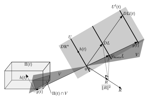
Figure 7: The structure of the configuration space $\mathbb{R}^{m}$ when $q=1,{\rm dim}\,U=1,{\rm dim}\,V=2$. The right side of the figure shows how the vector $g(t)$ is obtained and the left side shows how the moving set $\Pi(t)\cap V$ is defined.

Compliance with Ethical Standards

Conflict of Interest: The authors have no conflict of interest.

References

- [1] S. Adly, M. Ait Mansour, L. Scrimali, Sensitivity analysis of solutions to a class of quasi-variational inequalities. Boll. Unione Mat. Ital. Sez. B Artic. Ric. Mat. (8) 8 (2005), no. 3, 767–771.
- [2] R. B. Bapat, Graphs and matrices. Universitext. Springer, London; Hindustan Book Agency, New Delhi, 2010. x+171 pp.
- [3] T. R. Bieler, N. T. Wright, F. Pourboghrat, C. Compton, K. T. Hartwig, D. Baars, A. Zamiri, S. Chandrasekaran, P. Darbandi, H. Jiang, E. Skoug, S. Balachandran, G. E. Ice, W. Liu, Physical and mechanical metallurgy of high purity Nb for accelerator cavities, Physical Review Special Topics – Accelerators and Beams 13 (2010) 031002.
- [4] I. Blechman, Paradox of fatigue of perfect soft metals in terms of micro plasticity and damage, Int. J. Fatigue, in press (2018). https://doi.org/10.1016/j.ijfatigue.2018.10.017
- [5] D. Bremner, K. Fukuda, A. Marzetta, Primal-dual methods for vertex and facet enumeration. ACM Symposium on Computational Geometry (Nice, 1997). Discrete Comput. Geom. 20 (1998), no. 3, 333–357.
- [6] B. Brogliato, Absolute stability and the Lagrange-Dirichlet theorem with monotone multivalued mappings, Syst. Control Lett. 51 (2004) 343–353.
- [7] B. Brogliato and W. P. M. H. Heemels, Observer Design for Lur’e Systems With Multivalued Mappings: A Passivity Approach, IEEE Transactions on Automatic Control 54 (2009), no. 8, 1996–2001.
- [8] M. Brokate, J. Sprekels, Hysteresis and Phase Transitions, Springer, 1996.
- [9] G. A. Buxton, C. M. Care, D. J. Cleaver, A lattice spring model of heterogeneous materials with plasticity. Modelling and simulation in materials science and engineering, 9 (2001), no. 6, 485–497.
- [10] R. Cang, Y. Xu, S. Chen, Y. Liu, Y. Jiao, M. Y. Ren, Microstructure Representation and Reconstruction of Heterogeneous Materials via Deep Belief Network for Computational Material Design. Journal of Mechanical Design 139 (2017), no. 7, 071404.
- [11] H. Chen, E. Lin, Y. Liu, A novel Volume-Compensated Particle method for 2D elasticity and plasticity analysis, International Journal of Solids and Structures 51 (2014), no. 9, 1819–1833.
- [12] G. Colombo, R. Henrion, R.; N. D. Hoang, B. S. Mordukhovich, Optimal control of the sweeping process over polyhedral controlled sets. J. Differential Equations 260 (2016), no. 4, 3397–3447.
- [13] John B. Conway. A Course in Functional Analysis. Second Edition. Springer, 1997.
- [14] C. O. Frederick, P. J. Armstrong, Convergent internal stresses and steady cyclic states of stress. J. Strain Anal. 1 (1966), no. 2, 154–159.
- [15] S. H. Friedberg, A. J. Insel, L. E. Spence, Linear Algebra, 4th Edition, Prentice-Hall of India, New Delhi, 2004.
- [16] G. Garcea, L. Leonetti, A unified mathematical programming formulation of strain driven and interior point algorithms for shakedown and limit analysis. Internat. J. Numer. Methods Engrg. 88 (2011), no. 11, 1085–1111.
- [17] W. Han, B. D. Reddy, Plasticity. Mathematical theory and numerical analysis. Second edition. Interdisciplinary Applied Mathematics, 9. Springer, New York, 2013. xvi+421 pp.
- [18] M. Heitzer, G. Pop, M. Staat, Basis reduction for the shakedown problem for bounded kinematic hardening material. J. Global Optim. 17 (2000), no. 1-4, 185–200.
- [19] H. R. Henriquez, M. Pierri, P. Taboas, On S-asymptotically -periodic functions on Banach spaces and applications. J. Math. Anal. Appl. 343 (2008), no. 2, 1119–1130.
- [20] D. W. Holmes, J. G. Loughran, H. Suehrcke, Constitutive model for large strain deformation of semicrystalline polymers, Mech Time-Depend Mater 10 (2006) 281–313.
- [21] H. Hubel, Simplified Theory of Plastic Zones, Springer, 2015.
- [22] A. Isidori, Nonlinear control systems. An introduction. Second edition. Communications and Control Engineering Series. Springer-Verlag, Berlin, 1989. xii+479 pp.
- [23] M. Jirasek, Z. P. Bazant, Inelastic Analysis of Structures. London: J. Wiley & Sons, 2002.
- [24] P. Jordan, A. E. Kerdok, R. D. Howe, S. Socrate, Identifying a Minimal Rheological Configuration: A Tool for Effective and Efficient Constitutive Modeling of Soft Tissues, Journal of Biomechanical Engineering – Transactions of the ASME 133 (2011), no. 4, 041006.
- [25] M. Kamenskii, O. Makarenkov, L. Niwanthi Wadippuli, P. Raynaud de Fitte, Global stability of almost periodic solutions to monotone sweeping processes and their response to non-monotone perturbations. Nonlinear Anal. Hybrid Syst. 30 (2018) 213–224.
- [26] M. Krasnosel’skii, A. Pokrovskii, Systems with Hysteresis, Springer, 1989.
- [27] P. Krejci, Hysteresis, Convexity and Dissipation in Hyperbolic Equations. Gattotoscho, 1996.
- [28] P. Krejci, A. Vladimirov, Polyhedral sweeping processes with oblique reflection in the space of regulated functions. Set-Valued Anal. 11 (2003), no. 1, 91–110.
- [29] M. Kunze, M. D. P. Monteiro Marques, An introduction to Moreau’s sweeping process. Impacts in mechanical systems (Grenoble, 1999), 1-60, Lecture notes in phys., 551, Springer, Berlin, 2000.
- [30] R. I. Leine, N. van de Wouw, Stability and convergence of mechanical systems with unilateral constraints, Lecture Notes in Applied and Computational Mechanics, 36. Springer-Verlag, Berlin, 2008. xiv+236 pp.
- [31] R. I. Leine, N. van de Wouw, Uniform convergence of monotone measure differential inclusions: with application to the control of mechanical systems with unilateral constraints. Internat. J. Bifur. Chaos Appl. Sci. Engrg. 18 (2008), no. 5, 1435–1457.
- [32] H. X. Li, Kinematic shakedown analysis under a general yield condition with non-associated plastic flow, International Journal of Mechanical Sciences 52 (2010) 1–12.
- [33] C. W. Li, X. Tang, J. A. Munoz, J. B. Keith, S. J. Tracy, D. L. Abernathy, B. Fultz, Structural Relationship between Negative Thermal Expansion and Quartic Anharmonicity of Cubic , Physical Review Letters 107 (2011) 195504.
- [34] J. A. C Martins, M. D. P Monteiro Marques, A. Petrov, On the stability of quasi-static paths for finite dimensional elastic-plastic systems with hardening, ZAMM Z. Angew. Math. Mech. 87 (2007), no. 4, 303–313.
- [35] J. L. Massera, The existence of periodic solutions of systems of differential equations, Duke Math. J. 17 (1950) 457–475.
- [36] J.-J. Moreau, On unilateral constraints, friction and plasticity. New variational techniques in mathematical physics (Centro Internaz. Mat. Estivo (C.I.M.E.), II Ciclo, Bressanone, 1973), pp. 171-322. Edizioni Cremonese, Rome, 1974.
- [37] L. Narici, E. Beckenstein, Topological vector spaces. Second edition. Pure and Applied Mathematics (Boca Raton), 296. CRC Press, Boca Raton, FL, 2011. xviii+610 pp.
- [38] C. Polizzotto, Variational methods for the steady state response of elastic–plastic solids subjected to cyclic loads, International Journal of Solids and Structures 40 (2003), no. 11, 2673–2697.
- [39] A. R. S. Ponter, H. Chen, A minimum theorem for cyclic load in excess of shakedown, with application to the evaluation of a ratchet limit, Eur. J. Mech. A/Solids 20 (2001) 539–553.
- [40] R. T. Rockafellar, Convex analysis. Princeton Mathematical Series, No. 28 Princeton University Press, Princeton, N.J. 1970 xviii+451 pp.
- [41] J. Schwiedrzik, R. Raghavan, A. Burki, V. LeNader, U. Wolfram, J. Michler, P. Zysset, In situ micropillar compression reveals superior strength and ductility but an absence of damage in lamellar bone, Nature Materials 13 (2014), no. 7, 740–747.
- [42] E. Svanidze, T. Besara, M. F. Ozaydin, C. S. Tiwary, J. K. Wang, S. Radhakrishnan, S. Mani, Y. Xin, K. Han, H. Liang, T. Siegrist, P. M. Ajayan, E. Morosan, High hardness in the biocompatible intermetallic compound , Science Advances 2 (2016), no. 7, e1600319.
- [43] A. Visintin, Differential Models of Hysteresis, Springer, 1994.
- [44] D. Weichert, G. Maier (Eds.), Inelastic behavior of structures under variable repeated loads, Springer, New York, 2002.
- [45] J. Zhang, B. Koo, Y. Liu, J. Zou, A. Chattopadhyay, L. Dai, A novel statistical spring-bead based network model for self-sensing smart polymer materials, Smart Mater. Struct. 24 (2015) 085022.
- [46] N. Zouain, R. SantAnna, Computational formulation for the asymptotic response of elastoplastic solids under cyclic loads, European Journal of Mechanics A/Solids 61 (2017) 267–278.