A systematic construction of parity-time ($\cal PT$)-symmetric and non-$\cal PT$-symmetric complex potentials from the solutions of various real nonlinear evolution equations

Abstract

We systematically construct a distinct class of complex potentials including parity-time ($\cal PT$) symmetric potentials for the stationary Schrödinger equation by using the soliton and periodic solutions of the four integrable real nonlinear evolution equations (NLEEs) namely the sine-Gordon (sG) equation, the modified Korteweg-de Vries (mKdV) equation, combined mKdV-sG equation and the Gardner equation. These potentials comprise of kink, breather, bion, elliptic bion, periodic and soliton potentials which are explicitly constructed from the various respective solutions of the NLEEs. We demonstrate the relevance between the identified complex potentials and the potential of the graphene model from an application point of view.

1 Introduction

Over the last 15 years, the study of parity-time ($\cal PT$) symmetry has received wide attention in different branches of physics as they offered strong physical and mathematical insights. Initially, it emerged in quantum mechanics, where it has been shown that even if a Hamiltonian is not hermitian but admits $\cal PT$-invariance, then the energy eigenvalues are still real in case the $\cal PT$ symmetry is not broken spontaneously. This phenomenon was first observed in the pioneering work of Bender and Boettcher [1]. The fascinating properties of $\cal PT$-symmetric systems have paved the way for numerous developments in diverse areas of physics namely, quantum field theory, optics, photonics and Bose-Einstein condensates. Particularly, the concept of $\cal PT$ symmetry has inspired tremendous advances in optics because it has provided a multifaceted platform. In the realm of linear optics, theoretically complex $\cal PT$-symmetric potential has been studied in [2] followed by several experimental works on different optical systems, to name a few, coupled waveguide system [3], synthetic materials [4] and so on.

The next natural step is to explore various phenomena in nonlinear optical systems with $\cal PT$-symmetry. In nonlinear optics due to the interplay between the $\cal PT$ symmetric potentials and dispersion/diffraction as well as nonlinear effects, different types of localized structures (these structures are of relevance to the $\cal PT$ symmetric property) arise, such as solitons [5, 6, 7, 8], periodic waves [9], gap solitons [10] and vortices [11]. Particulary, the existence of different nonlinear localized modes has been studied analytically as well as numerically in the nonlinear Schrödinger (NLS) equation with complex $\cal PT$ symmetric periodic potential [12], Scarf-II potential[13], Gaussian potential [14], Bessel potential [15], Rosen-Morse Potential [16], harmonic potential[17]. In addition to these, nonlinear modes have been studied for other complex $\cal PT$- symmetric potentials bearing nonlinear optical systems like competing nonlinearity [18], saturable nonlinearity[19], logarithmically saturable nonlinearity [20]. On the other hand the complex potentials are used in BEC also to explore nonlinear localized modes [21].

These diversified studies clearly emphasise the need for the development of analytical procedure to construct many more $\cal PT$-symmetric potentials. In a classic work [22], Wadati has developed an interesting method to construct $\cal PT$-symmetric potentials of the form

$$V(x) = -q^{2}-iq_{x},$$ (1)

where the real function $q(x)$ is referred as potential base [22]. Recently, Wadati potentials have stated to receive renewed attention. Especially, the symmetry breaking of solitons has been observed in a class of non-$\cal PT$ Wadati like potentials beyond certain threshold value [23]. In another interesting work [24], nonlinear modes have been realized for the asymmetric waveguide profiles with Wadati potential. Stability analysis was also performed numerically for the Wadati like non-$\cal PT$ symmetric potentials [25]. More recently, the exact solutions of the Gross-Pitaevskii equation with Wadati like potential are constructed in [26].

Inspired by these recent advances, we obtain here a wide class of complex potentials including $\cal PT$ symmetric potentials for the linear Schrödinger equation with the aid of soliton and periodic solutions of different real integrable nonlinear evolution equations (NLEEs) namely the sine-Gordon (sG) equation, the modified Korteweg de Vries (mKdV) equation, combined mKdV-sG equation and the Gardner equation. All these equations are of considerable physical interest. These physically interesting NLEEs describe a plethora of phenomena in nonlinear science. For instance the sG system arises in a wide variety of physical systems, such as, long Josephson junction placed in an alternating electromagnetic field, elementary excitations of weakly pinned Fröhlich charge-density-wave condensates at low temperatures, DNA double helix [27] etc. The mKdV equation is useful in the study of the dust ion acoustic solitary waves in unmagnetized dusty plasma, Alfveń solitons in relativistic electron-positron plasma, the propagation of solitary waves in Schottky barrier transmission lines, in the models of traffic congestion [28] etc. Further, the mKdV-sG equation can be employed to describe physical situations such as nonlinear wave propagation in an infinite one dimensional anharmonic lattice and the propagation of ultrashort optical pulses solitons (or few cycle pulses solitons) in a Kerr medium [29]. Finally, the Gardner equation is useful in the study of propagation of ion-acoustic waves in plasmas and internal waves in a stratified ocean[30]. As mentioned above, optical systems can act as fertile ground for $\cal PT$ -symmetry properties. One of the main advantages of the systems that are presently under consideration in this paper is that except the Gardner equation, all the remaining equations arise in the context of nonlinear optics. Particularly, the propagation of few cycle pulses in Kerr media can be well described by using the mKdV, sG and mKdV-sG equations in the non-slowly varying envelope approximation [31].

In this paper we adapt the methodology developed by Wadati [22] to construct $\cal PT$ symmetric potentials. This method exploits the connection between time independent Schrödinger equation and the Zakharov-Shabat (Z-S) spectral problem to construct $\cal PT$-symmetric potentials using the several known periodic as well as hyperbolic soliton solutions of the above mentioned integrables NLEEs. In his pioneering work, Wadati has shown that the spatial evolution equations of the Z-S eigenvalue problem

$$v_{1x}+i\zeta v_{1} = qv_{2},$$ (2a)

$$v_{2x}-i\zeta v_{2} = -qv_{1}$$ (2b)

corresponding to the mKdV equation

$$q_{t}+6q^{2}q_{x}+q_{xxx}=0,$$ (2c)

can be transformed into the linear Schrödinger type eigenvalue problem featuring complex potential of the form (1) with eigenvalues being the square of the spectral parameter $\zeta^{2}$ of the Z-S problem. This complex potential is then explicitly constructed with the aid of the exact solutions of mKdV equation. The main point is that for those solutions which are derived from the IST method, one can immediately figure out if the energy eigenvalues of the stationary Schrödinger-like equation corresponding to these complex potentials are real or appear in complex conjugate pairs. This is an interesting result in the context of the complex $\cal PT$-invariant potentials as in that case one can then say if the corresponding eigenfunctions of the Schrödinger equation are $\cal PT$ invariant or not, i.e. if the $\cal PT$-symmetry is spontaneously broken or not. Here we wish to note that in a recent work [32], Barashenkov I V et al., have developed a procedure to construct $\cal PT$-symmetric Wadati type potentials for the Gross- Pitaevskii equation (nonlinear Schrödinger equation). In Ref.[32], the stationary nonlinear Schrödinger equation with unknown potential of Wadati type is systematically solved to explicitly construct the exact form of the Wadati potential and the nonlinear mode exhibiting such potentials is also found. In the present work, we have constructed general complex potentials of the linear Schrödinger equation with the aid of various known solutions of the integrable NLEEs like sG equation, mKdV equation, combined mKdV-sG equation and Gardner equation as explained above.

For the majority of the cases considered in this paper, one obtains $\cal PT$ invariant complex potentials but in certain cases one also obtains complex potentials which are not $\cal PT$ invariant. Especially, we consider the IST solutions for constructing complex potentials corresponding to the sG and the mKdV-sG systems. On the otherhand, Wadati has already considered [22] the potential based on the IST method solutions of the mKdV and the Gardner systems and constructed the corresponding complex potential as mentioned before. Hence, for completeness, we only focus our attention on the interesting solutions of the mKdV and the Gardner equation which are not obtained by the IST method. Finally, we also point out the possible relevance of some of the complex $\cal PT$-invariant solutions of the sG and the mKdV-sG systems in the context of the graphene system which is described by the Dirac equation. It is worth pointing out here that in the context of the same graphene system, the relevance of the complex $\cal PT$-symmetric potentials following from the solutions of the mKdV and the Gardner equations has been shown before [33].

This paper is organized as follows: In sec. 2, we construct $\cal PT$ symmetric potentials, both periodic and hyperbolic types, from the solution of sG equation. We show that in the special case of the breather solutions we obtain potentials which do not admit $\cal PT$ symmetry. We also show here the possible relevance of the obtained potentials from the sG equation in the context of the graphene model. In sec. 3, we apply the systematic method discussed in [22] to the mKdV equation and construct $\cal PT$ symmetric periodic as well as hyperbolic potentials. We then consider the combined mKdV-sG and Gardner equations in secs. 4 and 5 respectively and in both the cases we obtain complex $\cal PT$ invariant potentials. Our results are summarized in sec. 6.

2 Complex potentials from the solution of sine-Gordon equation

To start with, let us consider the ubiquitous sine-Gordon equation [34, 35]

$$u_{tt}-u_{xx}+\sin u=0\,.$$ (2d)

Here, the field $u(x,t)$ is real and the subscripts $x$ and $t$ denote partial derivatives with respect to space and time respectively. The field of the sG equation satisfies vanishing boundary condition, i.e., $u(x,t)\rightarrow 0$ at $x\rightarrow\pm\infty$. Eq. (2d) results from the compatibility condition of the famous Zakharov-Shabat (Z-S) $(2\times 2)$ problem with the following spatial and temporal evolution equations:

$$v_{1x}+i\zeta v_{1} = -qv_{2},\,$$ (2ea)

$$v_{2x}-i\zeta v_{2} = qv_{1}\,$$ (2eb)

and

$$v_{1t}=\left(\frac{i}{4\zeta}\right)\left(v_{1}\mbox{cos(u)}+v_{2}\mbox{sin(u)}\right),\,$$ (2ec)

$$v_{2t}=\left(\frac{i}{4\zeta}\right)\left(v_{1}\mbox{sin(u)}-v_{2}\mbox{cos(u)}\right),\,$$ (2ed)

where, $q=\frac{u_{x}}{2}$ and $\zeta$ is the spectral parameter which is in general complex. One can arrive at the following one dimensional stationary Schrödinger equation involving sine-Gordon potential $V^{(sG)}$ by differentiating Eqs. (2ea) and (2eb) with respect to $x$ and by introducing new eigenfunctions $\phi_{1}=v_{2}-iv_{1}$ and $\phi_{2}=v_{2}+iv_{1}$:

$$-\frac{d^{2}\phi_{1}}{dx^{2}}+V^{(sG)}\phi_{1} = \zeta^{2}\phi_{1},\,$$ (2efa)

$$-\frac{d^{2}\phi_{2}}{dx^{2}}+V^{*(sG)}\phi_{2} = \zeta^{2}\phi_{2},\,$$ (2efb)

where $*$ denotes the complex conjugation. The exact expressions for $V^{(sG)}$ is given by,

$$V^{(sG)}=-\frac{(u_{x})^{2}}{4}-i\frac{u_{xx}}{2}\equiv V_{R}(x)+iV_{I}(x)\,.$$ (2efg)

Thus the Hamiltonian consists of the complex potential that is furnished by the exact solution $u(x,t)$ of the sG equation. Though $u(x,t)$ depends on $t$, the energy spectrum of the Z-S problem (i.e. $\zeta^{2}$) is independent of $t$, which implies that $t$ can be viewed as a deformation parameter. Correspondingly the various solutions $u(x,t)$ of the sG Eq. (2d) generate deformable potentials $V(x,t)$ with real spectra if $\zeta$ is either real or purely imaginary. Hence the initial time and the solution parameters can be chosen appropriately such that solution is independent of time during the construction of potentials [36]. It should be noted that the real and imaginary parts of the complex potential associated with the sG equation are obtained from the real function $u(x,t)$. Thus it is the real solution $u(x,t)$ of the sG Eq. (2d) which determines the complex potential $V^{(sG)}(x,t)$ of the sG equation [22].

We remark that the real energy eigenvalues of the sG equation imply unbroken $\cal PT$ -symmetry whereas the complex conjugate pairs of energy eigenvalues of the sG equation lead to the spontaneous breaking of the $\cal PT$ -symmetry.

2.1 Relevance of the sG in the context of Dirac equation for the Graphene model

At this stage it is worth pointing out one possible application of the complex potentials obtained from the various solutions of the sG equation. In this regard, we wish to point out that very recently in Ref [33] a close connection has been established between the Dirac equation for the graphene model and the mKdV and the Gardner equations. Such a connection was established by showing that the solutions of these NLEEs can actually act as electrostatic potentials of the Dirac equation for the charge carriers in graphene at zero energy state. Along those lines, in order to realize the existence of similar connection between the graphene model and the solution of the sG potential, we first consider the following equation describing the motion of electrons in graphene in the presence of an electrostatic field [37]

$$\left[v_{F}(\sigma_{x}p_{x}+\sigma_{y}p_{y})\right]\psi+U(x,y)\psi=E\psi.$$ (2efh)

Here $p_{x}=-i\frac{\partial}{\partial x}$, $p_{y}=-i\frac{\partial}{\partial y}$, $v_{F}$, $U(x,y)$ and $E$ are the momentum operators in the $x$ and $y$ directions, the Fermi velocity, the potential energy and energy eigenvalue respectively. The wavefunction is chosen to be of the following form

$$\psi(x)=\Bigg{(}\begin{array}[]{c}\psi_{A}\\ \psi_{B}\\ \end{array}\Bigg{)}e^{ik_{y}y},$$ (2efk)

where $k_{y}$ is the wave vector of the $y$-component and the potential $U$ is assumed to depend only upon the $x$-coordinate. Substituting Eq. (2efk) into Eq. (2efh) and introducing the new eigenfunctions $\psi_{1,2}=(\psi_{A}\pm\psi_{B})$, we obtain

$$-\frac{d^{2}\psi_{1}}{dx^{2}}-\left((V(x)-\epsilon)^{2}+i\frac{dV}{dx}\right)\psi_{1}=-k_{y}^{2}\psi_{1},$$ (2efla)

$$-\frac{d^{2}\psi_{2}}{dx^{2}}-\left((V(x)-\epsilon)^{2}-i\frac{dV}{dx}\right)\psi_{2}=-k_{y}^{2}\psi_{2},$$ (2eflb)

where $V(x)=\frac{U(x)}{v_{F}}$ and $\epsilon=\frac{E}{v_{F}}$. To bring out the connection between Eqs. (10) and Eqs. (6), for zero energy states of graphene ($\epsilon=0$), we make the replacement $\psi_{1,2}\leftrightarrow\phi_{1,2}$ and $-k^{2}_{y}\leftrightarrow\zeta^{2}$. Then we notice that the resulting equations become identical for the choice $V(x)=\frac{u_{x}}{2}$. This gives the connection between the potential of the graphene model and the solution $u$ of the sG equation. In its original variables, the potential reads as

$$U(x)=\frac{v_{F}u_{x}}{2}.$$ (2eflm)

Note that this graphene potential is distinctly different from the previously reported potentials obtained from the mKdV and the Gardner system in [33]. This clearly demonstrates that the various solutions of the sG equation can furnish distinct exactly solvable electrostatic potentials for the graphene system corresponding to zero energy states. Going one step further than in [33], we find that for arbitrary energy states (with particular value for $\epsilon$) the connection between Eqs. (2efa) and (2efb) and Eqs. (2efla) and (2eflb) holds good for $V(x)=\frac{u_{x}}{2}+\epsilon$.

2.2 Construction of complex potentials

Now, we return to our main task and proceed to construct the complex potentials by using the exact solutions $u(x,t_{0})$, (where $t_{0}$ is the initial time) of the sG equation. The integrable sG equation admits the following N-kink soliton solution which is obtained by the IST method [38]

$$u(x,t) = \cos^{-1}\left[1+2\left(\frac{\partial^{2}}{\partial t^{2}}-\frac{\partial^{2}}{\partial x^{2}}\right)\ln f(x,t)\right],\,$$ (2efln)

where $f(x,t)=\det(M(x,t))$ in which the elements $M_{ij}$ of the $N\times N$ square matrix $M$ can be expressed as $\frac{\left(a_{i}a_{j}\right)^{\frac{1}{2}}}{a_{i}+a_{j}}\left[e^{\theta_{i}}+(-1)^{i+j}e^{-\theta_{j}})\right]$ in which $\theta_{i}$ = $\frac{1}{2}\left(a_{i}+\frac{1}{a_{i}}\right)x+\delta_{i}(t)$ and $\delta_{i}(t)$ can be expressed as $\frac{1}{2}\left(a_{i}-\frac{1}{a_{i}}\right)t+\rho_{i}~{}~{}(i,j=1,2,...,N)$ with arbitrary constants $a_{i}$ and $\rho_{i}$. Remarkably, it is well known that for the $N$-soliton solution the parameter $\zeta$ is pure imaginary and hence the energy $\zeta^{2}$ of the Schrödinger-like Eq. (2efa) is real. In the case of one and two soliton solutions we now explicitly show that the corresponding complex potential $V^{(SG)}$ is $\cal PT$ invariant thereby demonstrating that in these cases the $\cal PT$ symmetry is not spontaneously broken. We conjecture that the same is also true in the case of $N$ soliton solutions of the sG Eq. (2d). In addition to that, one can use the recently reported degenerate multi-soliton and multi-breather solutions [39], to construct the complex potentials.

2.2.1 One-kink (or Scarf-II) potential for $N=1$

We now write down the exact one-kink solution of the sG equation resulting from Eq. (2efln) for $N=1$

$$u(x,t)=4\tan^{-1}\left(e^{\theta_{1}}\right)\,,$$ (2eflo)

where, $\theta_{1}=\frac{1}{2}\left(a_{1}+\frac{1}{a_{1}}\right)x+\delta_{1}(t)$, $\delta_{1}(t)=\frac{1}{2}\left(a_{1}-\frac{1}{a_{1}}\right)t+\rho_{1}$. By choosing the initial time $t_{0}$ such that $\delta_{1}(t_{0})=\frac{1}{2}\left(a_{1}-\frac{1}{a_{1}}\right)t_{0}+\rho_{1}=0$, we obtain the same solution (2eflo) but with $\theta_{1}=\frac{1}{2}\left(a_{1}+\frac{1}{a_{1}}\right)x$. Then from (2efg) we construct the one-kink potential as

$$V^{(sG)}(x)=-\frac{1}{4}\left(a_{1}+\frac{1}{a_{1}}\right)^{2}\Big{[}\mbox{sech}^{2}(\theta_{1})+i\tanh(\theta_{1})~{}\mbox{sech}(\theta_{1})\Big{]}.$$ (2eflp)

This type of potential is referred as ($\cal PT$-symmetric) Scarf-II potential. It has other names too such as hyperbolic Scarf potential or Gendenshtein potential [40]. The Scarf-II potential is characterized by the same real component as that of complex Rosen-Morse potential but with different imaginary part. Interestingly, defocusing Kerr media featuring Scarf-II potential can support bright-soliton[41]. Possibility of gray soliton in defocusing media with Scarf-II potential has also been analysed numerically in [13]. This Scarf-II potential is clearly $PT$-invariant. Further, the $\cal PT$-symmetry is unbroken spontaneously since this potential (which admits one bound state) has real energy eigenvalue $E^{(sG)}=-a_{1}^{2}$, since from the IST method it is well known that $\zeta=ia_{1}$.

It may be noted here that in spite of the alteration of the parameter $a_{1}$, the shape of the Scarf-II potential remains unchanged. Further, the real and the imaginary parts of the Scarf-II potential vanish at $x=\pm\infty$.

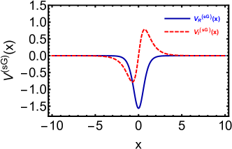
Figure 1: Real part (solid blue line) and imaginary part (red-dashed line) of the one-kink potential (2eflp) for $a_{1}=-0.5$.

To illustrate the nature of the potential, we display, the real part (solid blue line) and imaginary part (red-dashed line) of the Scarf-II potential in Fig. 1.

2.2.2 Two-kink potential for $N=2$

Next we shift our attention to the $N=2$ case, i.e. two-kink soliton solution of the sG equation obtained from Eq. (2efln)

$$u(x,t)=4\tan^{-1}\left[a\sinh\left(b\right)\mbox{sech}\left(c\right)\right],$$ (2eflq)

where, $a=\left(\frac{a_{1}-a_{2}}{a_{1}+a_{2}}\right)$; $b=\frac{1}{2}\left(\theta_{1}+\theta_{2}\right)$ and $c=\frac{1}{2}\left(\theta_{1}-\theta_{2}\right)$. Here $\theta_{1,2}$ is expressed as $\frac{1}{2}\left(a_{1,2}+\frac{1}{a_{1,2}}\right)x+\delta_{1,2}(t)$, $\delta_{1,2}(t)=\frac{1}{2}\left(a_{1,2}-\frac{1}{a_{1,2}}\right)t+\rho_{1,2}$. The time dependence in (2eflq) can be eliminated by choosing the initial time $t=t_{0}$, as $\delta_{1,2}(t_{0})=\frac{1}{2}\left(a_{1,2}-\frac{1}{a_{1,2}}\right)t_{0}+\rho_{1,2}=0$. The resulting solution bears the same form as in (2eflq), while $\theta_{1,2}=\frac{1}{2}\left(a_{1,2}+\frac{1}{a_{1,2}}\right)x$ and ultimately, the parameters $b$ and $c$ are time independent. Then, we construct two-kink potential from (2efg) as

$$V^{(sG)}(x)=\frac{1}{4}\Bigg{[}\Bigg{(}4a\frac{\big{(}b~{}\mbox{sech}(c)\cosh(b)-c~{}\sinh(b)\mbox{sech}(c)\tanh(c)\big{)}}{1+\big{(}a\sinh(b)\mbox{sech}(c)\big{)}^{2}}\Bigg{)}^{2}$$

$$-i\Bigg{(}2\frac{\mbox{d}}{\mbox{dx}}\Bigg{(}4a\frac{\big{(}b~{}\mbox{sech}(c)\cosh(b)-c~{}\sinh(b)\mbox{sech}(c)\tanh(c)\big{)}}{1+\big{(}a\sinh(b)\mbox{sech}(c)\big{)}^{2}}\Bigg{)}\Bigg{)}\Bigg{]}.$$ (2eflr)

Note that this two-kink potential is also $\cal PT$ -invariant and the $\cal PT$ -symmetry is unbroken since from the IST method it is well known that this potential admits two bound states with real energy eigenvalues $E^{(sG)}_{1}=-a^{2}_{1}$ and $E^{(sG)}_{2}=-a^{2}_{2}$.

It is amusing to note that unlike the one-kink potential, the shape of the two-kink potential can be altered by changing the values of the soliton parameters $a_{1}$ and $a_{2}$.

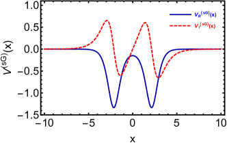
Figure 2: Real part (solid blue line) and imaginary part (red-dashed line) of the two-kink potential (2.2.2) for $a_{1}=0.5$ and $a_{2}=0.7$.

In order to analyse the nature of the two-kink potential, we have plotted the real part (continuous blue line) and the imaginary part (red-dashed line) of the two-kink potential in Fig. 2.

2.2.3 Breather type potential

Next, we move on to construct potential following from the celebrated breather solution of the sG Eq. (2d). In this connection, we start with the breather solution of the sG equation [38] obtained by the IST method:

$$u(x,t)=4\tan^{-1}\left(a_{0}~{}\mbox{sech}\left(a_{3}x+\delta_{3}\right)~{}\cos\left(a_{4}x+\delta_{4}\right)\right),$$ (2efls)

where $a_{0}=\left(\frac{\eta}{\xi}\right)$, $a_{3}=\left(\frac{\eta~{}\nu}{2}\right)$ and $a_{4}=\left(\frac{\xi(\nu-4)}{2}\right)$, in which $\eta$, $\xi$ and $\nu$ are real parameters, $\delta_{3}$ and $\delta_{4}$ are expressed as $-(4-\nu)t-a_{3}x_{0}\nu$ and $\left(\frac{\xi}{2}\right)\nu(t-\tau_{0})$ respectively. Here, $x_{0}$ and $\tau_{0}$ are arbitrary constants. By considering the initial time $t_{0}$ such that $\delta_{3}(t_{0})=-(4-\nu)t_{0}-a_{3}x_{0}\nu=0$ and $\delta_{4}(t_{0})=\left(\frac{\xi}{2}\right)\nu(t_{0}-\tau_{0})=0$, the solution (2efls) becomes

$$u(x)=4\tan^{-1}\left(a_{0}~{}\mbox{sech}\left(a_{3}\right)\cos\left(a_{4}x\right)\right).$$ (2eflt)

The breather solution (2eflt) is obtained by the IST method which involves complex conjugate pairs of eigenvalues. The breather potential resulting from solution (2eflt) is given below,

$$V^{(sG)}(x)=-\frac{(4~{}a_{0}^{2}~{}\mbox{sech}^{2}(a_{3}x)~{}(a_{4}~{}\sin(a_{4}x)+a_{3}~{}\cos(a_{4}x)\tanh(a_{3}x))^{2})}{(1+a^{2}\cos^{2}(a_{4}x)\mbox{sech}^{2}(a_{3}x))^{2}}+$$

$$+2i\frac{\mbox{d}}{\mbox{dx}}\Bigg{(}\frac{(a_{0}~{}\mbox{sech}(a_{3}x)~{}(a_{4}~{}\sin(a_{4}x)+a_{3}~{}\cos(a_{4}x)\tanh(a_{3}x))}{(1+a^{2}\cos^{2}(a_{4}x)\mbox{sech}^{2}(a_{3}x)}\Bigg{)}\Bigg{]},\qquad\qquad$$ (2eflu)

The above complex breather-type potential does not have the $\cal PT$ -symmetry. This non-$\cal PT$ -symmetric potential admits robust shape for all real values of $\xi$ and $\eta$. One can easily notice that the real part and imaginary parts of this breather potential asymptotically vanish. It is amusing to note that while the soliton solutions lead to a potential with $\cal PT$-symmetry, the breather solution fails to result in such $\cal PT$ -symmetric potential. This is of course perfectly understandable as the breather solution (2efls), is obtained by considering the eigenvalues as complex conjugate pairs which results in complex spectral parameters $\zeta_{1}=\xi+i\eta$ and $\zeta_{2}=\xi-i\eta$. The corresponding eigenvalues are thus $E_{1}=\xi^{2}-\eta^{2}+2i\xi\eta$ and $E_{2}=\xi^{2}-\eta^{2}-2i\xi\eta$.

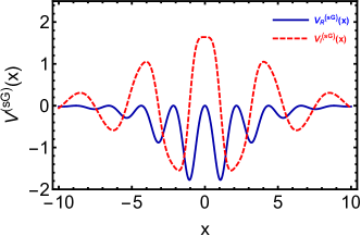
Figure 3: Real part (solid blue line) and imaginary part (red-dashed line) of the breather potential (2.2.3) for $\eta=0.5$, $\xi=1$, $\nu=1.2$.

In Fig. 3, we depict the real part (solid blue line) and imaginary part (red-dashed line) of breather type potential respectively. Notice that both the real and the imaginary parts are symmetric function.

2.2.4 Periodic two kink potential

Now, we focus our attention to construct periodic two kink potential from the periodic two kink solution of the sG equation. The periodic two kink solution of the sG equation (2d) can be written as [42]

$$u(x,t)=4\tan^{-1}[\mbox{sd}(ax+\delta_{5}(t),k)~{}\mbox{cn}(cx+\delta_{6}(t),m)]\,.$$ (2eflv)

The constraint conditions are expressed as $a=m~{}c$; $b=-d=\Big{(}\frac{m^{2}}{2m^{2}k^{2}-3m^{2}+1}\Big{)}$ and $m=\pm\frac{1}{\sqrt{1+k^{2}-k^{4}}}$. Here $\delta_{5}(t)$ and $\delta_{6}(t)$ are given by $bt+s_{0}$ and $dt+r_{0}$ respectively, in which $s_{0}$ and $r_{0}$ are arbitrary constants. Here cn(cx,k), and $\mbox{sd}(bx,m)\Big{(}\equiv\frac{\mbox{sn}(bx,m)}{\mbox{dn}(bx,m)}\Big{)}$ are Jacobi elliptic functions with modulii k and m, respectively. These elliptic functions sn, cn and dn are doubly periodic functions having periods $4K$, $4K$ and $2K$ respectively. One can easily obtain the following solution from solution (2eflv) by considering the initial time $t_{0}$ such that $\delta_{5}(t_{0})=bt_{0}+s_{0}=0$ and $\delta_{6}(t_{0})=dt_{0}+r_{0}=0$

$$u(x)=4\tan^{-1}[\mbox{sd}(ax,k)~{}\mbox{cn}(cx,m)]\,.$$ (2eflw)

Using solution (2eflw), we obtain the following complex potential

$$V^{(SG)}(x)=V^{(sG)}_{R}(x)+iV^{(sG)}_{I}(x)\,,$$ (2eflxa)

where the real and imaginary parts of the periodic potential from the periodic solution of the sG equation are given respectively by

$$V^{(sG)}_{R}(x)=-4\Big{(}\frac{a~{}\zeta_{1}~{}\mbox{nd}(ax,k)-c~{}\zeta_{2}~{}\mbox{sn}(cx,m)}{(1+\mbox{cn}^{2}(cx,m)~{}\mbox{sd}^{2}(ax,k))}\Big{)}^{2}$$ (2eflxb)

and

$$V^{(sG)}_{I}(x)=-2\frac{\mbox{d}}{\mbox{dx}}\Big{(}\frac{a~{}\zeta_{1}~{}\mbox{nd}(ax,k)-c~{}\zeta_{2}~{}\mbox{sn}(cx,m)}{(1+\mbox{cn}^{2}(cx,m)~{}\mbox{sd}^{2}(ax,k))}\Big{)}.$$ (2eflxc)

Here $\zeta_{1}=\mbox{cd}(ax,k)~{}\mbox{cn}(cx,m)$, $\zeta_{2}=\mbox{dn}(cx,m)~{}\mbox{sd}(ax,k)$ and also $\mbox{cd}(bx,k)\Big{(}\equiv\frac{\mbox{cn}(bx,k)}{\mbox{dn}(bx,k)}\Big{)}$ and $\mbox{nd}(bx,k)\Big{(}\equiv\frac{1}{\mbox{dn}(bx,k)}\Big{)}$. It is easily seen that this potential respects $\cal PT$ -symmetry. The obvious question is if the $\cal PT$-symmetry is spontaneously unbroken or not. Unfortunately, since the periodic two-soliton solution is not obtained through the IST method, one does not have the information about the corresponding eigenvalues. However, there are two reasons because of which we believe that in this case too the $\cal PT$-symmetry is not spontaneously broken. Firstly, in the limit when the periodic two-soliton solution goes over to the two-soliton solution (2eflq), we know that the $\cal PT$-symmetry is not spontaneously broken. Secondly, we have numerically calculated the low lying energy eigenvalues and they turn out to be real. It would be nice if one can rigorously show that even in this case the $\cal PT$-symmetry is not spontaneously broken.

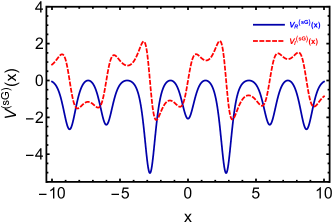
Figure 4: Real part (solid blue line) and imaginary part (red-dashed line) of the periodic two-kink potential (2eflxa) for $c=0.9$, $k=0.9$, $m=0.8$.

In Fig. 4, we display the real part (blue line) and imaginary part (red-dashed line) of periodic two-kink potential.

2.2.5 Periodic breather potential

In what follows, we discuss the construction of the periodic breather potential following from the periodic breather solution of the sG equation. The periodic breather solution of the sG equation is given by [42]

$$u(x,t)=4\tan^{-1}[\mbox{cd}(ax+\delta_{5}(t),k)~{}\mbox{dn}(cx+\delta_{6}(t),m)]\,.$$ (2eflxya)

This solution (2eflxya) reduces to the breather solution (2efls) in the limit $$m\rightarrow 1 k\rightarrow 0 a=c b=-\frac{1}{2(2-m^{2})a} d=\pm\frac{1}{2(2-m^{2})a} t_{0} \delta_{5}(t_{0})=bt_{0}+s_{0} \delta_{6}(t_{0})=dt_{0}+r_{0}$$ and . In the above solution, ; ; and we consider suitable initial time so as to make and to be zero. Then the solution (2eflxya) can be rewritten as

$$u(x)=4\tan^{-1}[\mbox{cd}(ax,k)~{}\mbox{dn}(cx,m)].$$ (2eflxyb)

The complex potential resulting for the above solution (2eflxyb) is

$$V^{(sG)}(x)=-\frac{1}{4}\Bigg{[}\Bigg{(}\frac{4a(k-1)\mbox{dn}(cx,m)~{}\zeta_{3}-c~{}m~{}\mbox{cd}(ax,k)~{}\zeta_{4}}{1+\mbox{cd}^{2}(ax,k)~{}\mbox{dn}^{2}(cx,m)}\Bigg{)}^{2}+$$

$$2i~{}\frac{\mbox{d}}{\mbox{dx}}\Bigg{(}\frac{4a(k-1)\mbox{dn}(cx,m)~{}\zeta_{3}-c~{}m~{}\mbox{cd}(ax,k)~{}\zeta_{4}}{1+\mbox{cd}^{2}(ax,k)~{}\mbox{dn}^{2}(cx,m)}\Bigg{)}\Bigg{]}.$$

Here the parameters $\zeta_{3}$ and $\zeta_{4}$ can be expressed as $\mbox{nd}(ax,k)~{}\mbox{sd}(ax,k)$ and $\mbox{cn}(cx,m)~{}\mbox{sn}(cx,m)$. It is clear that this complex periodic breather-type potential does not have $\cal PT$-symmetry. This non-$\cal PT$ -symmetric potential varies its profile as the parameters $a$ and $c$ are changed.

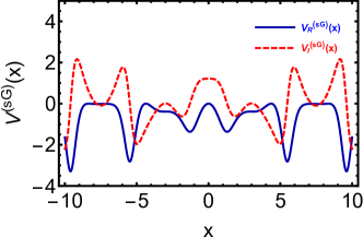
Figure 5: Real part (solid blue line) and imaginary part (red-dashed line) of the periodic breather potential (2.2.5) for $a=c=0.9$, $b=0.4$, $m=0.8$.

In Fig. 5, we display the real part (blue line) and imaginary part (red-dashed line) of periodic breather potential. This clearly shows the non-$\cal PT$ symmetric nature of potential.

3 Construction of complex potentials from the solution of modified KdV equation

After the detailed discussion about the various complex potentials following from the sG equation, we extend our approach to the integrable mKdV equation (2c). As mentioned in the introduction the construction of the $\cal PT$ -symmetric potentials for the mKdv equation has already been discussed by Wadati in his pioneering work [22]. However, it is limited to the case of one and two soliton potentials. It is of interest to construct the complex potentials from the solution of mKdV equation by considering various other interesting non-solitonic solutions like bion, elliptic bion and other periodic solutions [43]. Due to the physical importance of the above mentioned solutions, we extend the elegant theory developed by Wadati to construct potentials corresponding to other interesting solutions of the mKdV equation (2c).

Then by following the procedure outlined in section 2.1, we obtain the following complex potential for the linear Schrödinger equation by using the solution of the mKdV equation

$$V^{(mKdV)} = V^{(mKdV)}_{R}+iV^{(mKdV)}_{I}\equiv-q^{2}-iq_{x}.$$ (2eflxyaa)

Note that as in the sG case, this complex potential is generated by the real solution $q(x,t)$ of the mKdV equation. In what follows, we deal with special elliptic bion solution, bion solution, dnoidal, cnoidal and superposed elliptic solutions of the mKdV system.

3.1 Bion potential

We now consider the following interesting bion solution of the mKdV equation [43].

$$q(x,t)=-2\frac{\mbox{d}}{\mbox{dx}}\Big{[}\tan^{-1}(a~{}\sin(\alpha x+\rho_{4}(t))~{}\mbox{sech}(\beta x+\rho_{5}(t)))\Big{]}\,.$$ (2eflxyaba)

Here $$\rho_{4}(t) \rho_{5}(t) \upsilon t+a_{0} \varsigma t+b_{0} a=-\frac{\beta}{\alpha} \upsilon=(\alpha^{2}-3\beta^{2})\alpha \varsigma=(3\alpha^{2}-\beta^{2})\beta t_{0} \rho_{4}(t_{0})=\upsilon t_{0}+a_{0} \rho_{5}(t_{0})=\varsigma t_{0}+b_{0}$$ and are given as and respectively. The constraint conditions are , and . As before, by choosing the initial time such that and vanish, one can obtain the following stationary form

$$q(x)=-2\frac{d}{dx}\Big{[}\tan^{-1}(a~{}\sin(\alpha x)~{}\mbox{sech}(\beta x))\Big{]}\,.$$ (2eflxyabb)

This bion solution results in the following complex potential

$$V^{(mKdv)}(x)=\Bigg{[}-\Bigg{(}\frac{2a~{}\mbox{sech}(\beta x)(\alpha\cos(\alpha x)-\beta\sin(\alpha x)\tanh(\beta x))}{(1+a^{2}\mbox{sech}^{2}(x\beta)\sin^{2}(x\alpha))}\Bigg{)}^{2}$$

$$-i\frac{\mbox{d}}{\mbox{dx}}\Bigg{(}\frac{2a\mbox{sech}(\beta x)(\alpha\cos(\alpha x)-\beta\sin(\alpha x)\tanh(\beta x))}{(1+a^{2}\mbox{sech}^{2}(x\beta)\sin^{2}(x\alpha))}\Bigg{)}\Bigg{]}.$$ (2eflxyabac)

The above bion potential also possesses $\cal PT$ symmetry. Since it is not derived by the IST method, we do not know for sure its energy eigenvalues and hence it is not clear if the $\cal PT$-symmetry remains unbroken or not. We have numerically evaluated low lying eigenvalues and they are real thereby suggesting that in this case too the $\cal PT$-symmetry is not spontaneously broken. It would be nice if one can rigorously prove it.

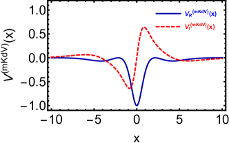
Figure 6: Real part (solid blue line) and imaginary part (red-dashed line) of bion potential for $\alpha=0.5$ and $\beta=0.3$.

A plot of the potential is given in Fig. 6 from where too it is clear that while the real part of the potential is symmetric, the imaginary part is antisymmetric.

3.2 Elliptic bion potential

We consider the following elliptic bion solution of the mKdV equation [43].

$$q(x,t)=-2\frac{\mbox{d}}{\mbox{dx}}\Big{[}\tan^{-1}(a~{}\mbox{sn}(\alpha x+\rho_{4}(t),k)~{}\mbox{dn}(\beta x+{\rho_{5}(t)},m))\Big{]}.$$ (2eflxyabada)

The parameters of solution (2eflxyabada) satisfy the relations, $$a=-\frac{\beta}{\alpha} \frac{\beta}{\alpha}=\left(\frac{k}{(1-m)}\right)^{\frac{1}{4}} \rho_{4,5}(t) \upsilon t+a_{0} \varsigma t+b_{0} \upsilon=(\alpha^{2}(1+k)-3\beta^{2}(2-m))\alpha \varsigma=(3\alpha^{2}(1+k)-\beta^{2}(2-m))\beta t_{0} \rho_{4}(t_{0})=\upsilon t_{0}+a_{0} \rho_{5}(t_{0})=\varsigma t_{0}+b_{0}$$; . Here the parameters are given as and respectively, in which the and . By considering initial time such that and vanish, we obtain the stationary version of (2eflxyabada) which reads as

$$q(x)=-2\frac{\mbox{d}}{\mbox{dx}}\Big{[}\tan^{-1}(a~{}\mbox{sn}(\alpha x,k)~{}\mbox{dn}(\beta x,m))\Big{]}\,.$$ (2eflxyabadb)

This elliptic bion solution results in the following complex potential

$$V^{(mKdV)}(x)=\Bigg{[}-\Bigg{(}\frac{2a~{}(m~{}\beta~{}\gamma_{2}~{}\mbox{sn}(~{}\beta x,m)-\alpha~{}\gamma_{1}~{}\mbox{dn}(\beta x,m))}{(1+a^{2}\gamma^{2})}\Bigg{)}^{2}$$

$$-i\frac{d}{dx}\Bigg{(}\frac{2a~{}(m~{}\beta~{}\gamma_{2}~{}\mbox{sn}(~{}\beta x,m)-\alpha~{}\gamma_{1}~{}\mbox{dn}(\beta x,m))}{(1+a^{2}\gamma^{2})}\Bigg{)}\Bigg{]}.$$ (2eflxyabadae)

Here the expressions for $\gamma$, $\gamma_{1}$ and $\gamma_{2}$ are $\mbox{dn}(\beta x,m)~{}\mbox{sn}(\alpha x,k)$, $\mbox{cn}~{}(\alpha x,k)~{}\mbox{dn}(\alpha x,k)$ and $\mbox{cn}(\beta x,m)~{}\mbox{sn}(\alpha x,k)$ respectively. It is easy to see that this elliptic bion potential is $\cal PT$ -symmetric. Since this solution is not derived by the IST method. We have no clue about the nature of its energy eigenvalues. Hence it is not clear if the $\cal PT$-symmetry remains unbroken or not. We have numerically evaluated few low lying eigenvalues which turn out to be real thereby suggesting that for this case also the $\cal PT$-symmetry is not spontaneously broken. A rigorous proof of this could be an interesting study.

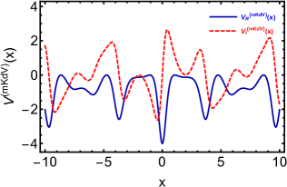
Figure 7: Real part (solid blue line) and imaginary part (red-dashed line) of elliptic bion potential (3.2) for $\alpha=1$; $m=0.8$ and $k=0.2$.

This elliptic bion potential is shown in Fig. 7 and it alters its profile as the parameters $\alpha$ and $\beta$ are varied as shown in Fig. 7.

3.3 Periodic potentials

The above construction procedure of complex potential from the solution of the mKdV system (2c) can be straightforwardly extended to the other periodic potentials like dnoidal, cnoidal and superposed elliptic solutions of the mKdV equation. We tabulate below these remaining solutions and the corresponding potentials for brevity in Table 1.

Table 1: Novel types of complex potentials for the mKdV equation

Type of	$q(x,t)$	$q(x)$	$V^{(mKdV)}(x)$	Constraints
solutions
dnoidal	$\mbox{A}~{}\mbox{dn}(\theta,m)$	$\mbox{A}~{}\mbox{dn}(\beta x,m).$	$\Big{[}-\mbox{A}^{2}~{}\mbox{dn}^{2}(\beta x,m)$	$A^{2}=\beta^{2}$
solution			$+i\mbox{A}~{}\mbox{m}~{}\beta\mbox{cn}(\beta x,m)$	$v=(2-m)\beta^{2}$
			$\mbox{sn}(\beta x,m)\Big{]}$
cnoidal	$\mbox{A}~{}\sqrt{m}~{}\mbox{cn}(\theta,m)$	$\mbox{A}~{}\sqrt{m}~{}\mbox{cn}(\beta x,m).$	$\Big{[}-\mbox{A}^{2}\mbox{m}~{}\mbox{cn}^{2}(\beta(x),m)$	$A^{2}=\beta^{2}$
solution			$+i\mbox{A}~{}\sqrt{m}~{}\beta\mbox{dn}(\beta(x),m)$	$v=(2m-1)\beta^{2}$
			$\mbox{sn}(\beta(x),m)\Big{]}$
Superposed	$\frac{A}{2}\Big{(}\mbox{dn}(\theta,m)\pm$	$\frac{A}{2}\Big{(}\mbox{dn}(\beta x,m)\pm$	$-\Bigg{[}\frac{A^{2}}{4}\Big{(}\mbox{dn}(\beta(x),m)$
			$\pm\sqrt{m}\mbox{cn}(\beta(x),m)\Big{)}^{2}$	$~{}A^{2}=\beta^{2}$
solution	$\sqrt{m}\mbox{cn}(\theta,m)\Big{)}$	$\sqrt{m}\mbox{cn}(\beta x,m)\Big{)}$	$\frac{iA}{2}\frac{\mbox{d}}{\mbox{dx}}\Big{(}\mbox{dn}(\beta(x),m)$	$v=\frac{(1+m)\beta^{2}}{2}$
			$\pm\sqrt{m}\mbox{cn}(\beta(x),m)\Big{)}\Bigg{]}$

In Table 1, $\theta=\beta(x+\rho_{5}(t))$, where $\rho_{5}(t)$ can be expressed as $(-vt+x_{0})$ ($x_{0}$ is a constant). In the second column of the Table 1, we present the time dependent elliptic solutions and we convert those solutions as time independent solutions (stationary solutions) in the third column by choosing the initial time $t_{0}$ appropriately such that $\rho_{4}(t_{0})=-vt_{0}+x_{0}=0$.

All the three elliptic potentials presented in Table 1 are $\cal PT$ -symmetric potentials. The obvious question is if the $\cal PT$-symmetry is spontaneously unbroken or not. Unfortunately, since these periodic soliton solutions are not obtained through the IST method, the nature of the corresponding eigenvalues can not be predicted. However, for two reasons we believe for these cases the $\cal PT$-symmetry not to be spontaneously broken. Firstly, in the limit $m=1$ when these periodic soliton solutions goes over to the one soliton solution and from the IST procedure we know that the eigenvalue is real and hence $\cal PT$-symmetry is not spontaneously broken. Secondly, we have numerically calculated the low lying energy eigenvalues for these three $\cal PT$-invariant potentials and they turn out to be real. It would be nice if one can rigorously show that even in these cases the $\cal PT$-symmetry is not spontaneously broken.

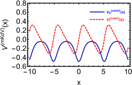
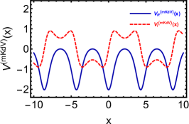
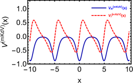
Figure 8: Real part (solid blue line) and imaginary part (red-dashed line) of the dnoidal potential (Left panel) for $A=0.7$, $\beta=1$ and $m=0.9$; cnoidal potential (middle-panel) for $A=1.5$, $\beta=1.2$ and $m=0.9$ and superposed potential (right-panel) for $A=1.1$, $\beta=1.5$ and $m=0.5$ respectively.

In Fig. 8 we have depicted the real and imaginary parts of the dnoidal (left-panel), cnoidal (middle-panel) and superposed potential (right-panel). All these potentials posses robust shape even if we change the corresponding solution parameters.

4 Construction of complex potentials from the solution of mKdV-sG equation

Now we extend our systematic construction of complex potentials from the solution of combined mKdV-sG system which is receiving attention recently [29]. As mentioned in the introduction, this system describes the propagation of few-optical-cycle pulses in a self-focusing Kerr medium which is of paramount of interest. The complete integrability of this physically interesting system has been proved by means of the IST method [29]. The mKdV-sG system is casted as

$$u_{xt}+\Upsilon\left(\frac{3}{2}(u_{x})^{2}u_{xx}+u_{xxxx}\right)-\Upsilon_{1}\sin(u)=0\,,$$ (2eflxyabadaf)

where the field $u$ is a function of $x$ and $t$. The constants $\Upsilon$ and $\Upsilon_{1}$ account for the dispersion and nonlinearity properties of the medium and are chosen to be one without loss of generality. The Lax pair for the system (2eflxyabadaf) is well known [29]. The spatial evolution equations for the mKdV-sG system and the sG system are identical albeit their time evolution differs. Hence the complex potential for the linear Schrödinger equation using solution of this mKdV-sG equation can be obtained following the procedure for the sG system given in section 2. In particular

$$V^{(mKdv-sG)}(x) = V^{(mKdv-sG)}_{R}(x)+iV^{(mKdV-sG)}_{I}(x),$$ (2eflxyabadaga)

where the constituent real and imaginary parts of the $$V^{(mKdV-sG)}(x)$$ are

$$V^{(mKdV-sG)}_{R}(x) = -\frac{u_{x}^{2}}{4},$$ (2eflxyabadagb)

$$V^{(mKdV-sG)}_{I}(x) = -\frac{u_{xx}}{2}.$$ (2eflxyabadagc)

Note that here the quantity $u$ corresponds to the solution of (2eflxyabadaf). Following the sG example, we can similarly correlate the potential of the graphene model with the solution of the mKdV-sG system. Not surprisingly, the connection between the potential of the graphene model and the solution of the mKdV-sG system looks similar to the sG case and is given by:

$$V(x)=\frac{u_{x}}{2}\,,$$ (2eflxyabadagah)

where $u$ is the solution of the mKdV-sG system (2eflxyabadaf). Hence the form of the potential will be entirely different from that of the sG case. This shows the existence of a host of complex exactly solvable potentials for the graphene model.

Like the sG case, for the integrable mKdV-sG equation too people have obtained N-kink soliton solution through the IST method. It turns out that in spite of having different mathematical form from the sG system mKdV-sG system still admits the same stationary form for the one kink soliton as the sG case which is given in Eq. (2eflo). So, here we skip the discussion about the one-kink soliton of the mKdv-sG system. However, the two- kink soliton of the mKdV-sG system has distinct form that of the sG system.

4.0.1 Two kink potential

In this subsection, we focus on the construction of the two kink $\cal PT$ -symmetric potential from the two kink solution of the mKdV-sG equation. This two kink solution of the mKdV-sG equation (2eflxyabadaf) reads as

$$u(x,t)=4\tan^{-1}\left[\frac{a_{11}\cosh((\eta_{2}-\eta_{1})x+\Lambda_{1}(t))}{\sinh((\eta_{1}+\eta_{2})x+\Lambda_{2}(t))}\right],$$ (2eflxyabadagaia)

where $$a_{11}=\sqrt{\frac{(\eta_{1}+\eta_{2})^{2}(c_{10}\eta_{1}+c_{20}\eta_{2})}{c_{10}c_{20}(\eta_{1}-\eta_{2})^{2}}} \eta_{1,2} \Lambda_{1}(t) \Lambda_{2}(t) (A_{20}-A_{10})t+s_{1} (A_{10}+A_{20})+r_{1} s_{1} r_{1} \frac{1}{2}\ln(\frac{c_{10}}{2\eta_{1}}-\frac{c_{20}}{2\eta_{2}}) \frac{1}{2}\ln(\frac{c_{10}c_{20}(\eta_{1}-\eta_{2})^{2}}{4\eta_{1}\eta_{2}(\eta_{1}+\eta_{2})^{2}}) c_{10} c_{20} t_{0} \Lambda_{1}(t_{0})=(A_{20}-A_{10})t_{0}+s_{1}\equiv 0 \Lambda_{2}(t_{0})=(A_{10}+A_{20})t_{0}+r_{1}\equiv 0$$ with being the solion parameters. The expressions for and are given by and , respectively in which and are expressed as and , respectively. Here and are real arbitrary parameters. One can easily reduce the following stationary solution from the solution (2eflxyabadagaia) by considering the initial time as and :

$$u(x)=4\tan^{-1}\left[\frac{a_{11}\cosh((\eta_{2}-\eta_{1})x)}{\sinh((\eta_{1}+\eta_{2})x)}\right].$$ (2eflxyabadagaib)

Using solution (2eflxyabadagaib), we obtain the following complex potential

$$V^{(mKdV-SG)}(x)=V^{(mKdV-sG)}_{R}(x)+iV^{(mKdV-sG)}_{I}(x),$$ (2eflxyabadagaiaja)

where the real and imaginary parts of the two kink potential from the two kink solution of mKdV-sG equation are expressed as

$$V^{(mKdV-sG)}_{R}(x)=-\frac{1}{4}\Bigg{[}\frac{a_{11}\mbox{csch}(b_{12}x)\Big{(}b_{11}~{}\sinh(b_{11}x)-b_{12}~{}\cosh(b_{11}x)\coth(b_{12}x)\Big{)}}{1+\Big{(}a_{11}\frac{\cosh(b_{11}x)}{\sinh(b_{12}x)}\Big{)}^{2}}\Bigg{]}^{2},$$

$$V^{(mKdV-sG)}_{I}(x)=-\frac{1}{2}\frac{\mbox{d}}{\mbox{dx}}\Bigg{[}\frac{a_{11}\mbox{csch}(b_{12}x)\Big{(}b_{11}~{}\sinh(b_{11}x)-b_{12}~{}\cosh(b_{11}x)\coth(b_{12}x)\Big{)}}{1+\Big{(}a_{11}\frac{\cosh(b_{11}x)}{\sinh(b_{12}x)}\Big{)}^{2}}\Bigg{]}.$$

Here $b_{11}=(\eta_{2}-\eta_{1})$,  $b_{12}=(\eta_{1}+\eta_{2})$. It is easy to check that this two-kink potential (2eflxyabadagaiaja) associated with mKdV-sG equation respects $\cal PT$ -symmetry and in fact the $\cal PT$-symmetry is not spontaneously broken. This is because, in the case of the two kink solution of the mKdV-sG system, it is well known that the spectral parameters ($\zeta_{1}$, $\zeta_{2}$) associated with the kink solution (2eflxyabadagaia) are purely imaginary ($i\eta_{1}$, $i\eta_{2}$) thereby resulting in real energy eigenvalues, $E_{1}=-\eta_{1}^{2}$ and $E_{2}=-\eta_{2}^{2}$.

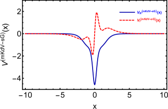
Figure 9: Real part (solid blue line) and Imaginary part (red-dashed line) of two kink potential from the two kink solution of the mKdV-sG equation for $c_{10}=0.5$, $c_{20}=1$, $\eta_{1}=0.5$ and $\eta_{2}=2.5$.

In Fig. 9 we plot the real and the imaginary parts of the two kink potential associated with mKdV-sG equation.

5 Construction of complex potentials from the solutions of Gardner equation

Finally, we shift our attention to another important soliton bearing integrable nonlinear model, i.e. the Gardner equation (GE). This equation is an extended version of the KdV equation with cubic nonlinearity. The integrability nature of the Gardner equation has been studied by using the IST method [44]. The $\cal PT$ -symmetric potential from the solution of the Gardner equation corresponding to the one-soliton solution has already been obtained in Ref. [22]. However, these are other interesting solutions of the Gardner equation such as two-soliton solution, breather and elliptic solutions and it is worth constructing complex potentials corresponding to some of these solutions. This is what we do in this section.

We consider the following dimensionless form of the Gardner equation [45]:

$$u_{t}+6\alpha_{1}uu_{x}+6\beta_{1}u^{2}u_{x}+u_{xxx}=0.$$ (2eflxyabadagaiajak)

Here $\alpha_{1}$ and $\beta_{1}$ are the nonlinearity coefficients. In order to construct the complex potentials of the Gardner equation, we consider its Lax representation. The spatial and temporal evolution equations of the Gardner equations are

$$v_{1x}+i\zeta v_{1} = qv_{2},$$ (2eflxyabadagaiajala)

$$v_{2x}-i\zeta v_{2} = rv_{1}$$ (2eflxyabadagaiajalb)

and

$$v_{1t}=(-4\eta^{3}+2\eta qr+rq_{x}-qr_{x})v_{1}+(-4\eta^{2}q-2\eta q_{x}+2q^{2}r-q_{xx})v_{2},$$ (2eflxyabadagaiajalc)

$$v_{2t}=(-4\eta^{2}r-2\eta r_{x}+2qr^{2}-r_{xx})v_{1}-(-4\eta^{3}+2\eta qr+rq_{x}-qr_{x})v_{2},$$ (2eflxyabadagaiajald)

where $q=u$ and $r=-(\alpha_{1}+\beta_{1}u)$. Following the procedure as outlined in section 2.1, one can construct the complex potentials for the linear Schrödinger equation using the solution of the Gardner equation

$$V^{(G)} = V^{(G)}_{R}+iV^{(G)}_{I},$$ (2eflxyabadagaiajalama)

where the real and imaginary parts of the potentials are given by

$$V_{R}^{(G)} = -\alpha_{1}u-\beta_{1}u^{2},$$ (2eflxyabadagaiajalamb)

$$V_{I}^{(G)} = -\sqrt{\beta_{1}}u_{x}.$$ (2eflxyabadagaiajalamc)

5.1 Two soliton potential

The two soliton solution of the Gardner equation has been derived using the Hirota’s bilinearization method. The form of the two soliton solution of the Gardner equation is [45]

$$u(x,t)=q_{0}\left[\frac{\cosh(k_{2}x-\rho_{7}(t))+\cosh(k_{1}x-\rho_{8}(t))}{\cosh(\kappa x-\rho_{9}(t))+\cosh(\kappa_{1}x-\rho_{10}(t))\cosh(\kappa_{1}x-\rho_{11}(t))}\right]-\frac{1}{2}.$$

Here, $$q_{0}=2\sqrt{k_{1}k_{2}a_{12}} \rho_{7,8}(t) \rho_{9}(t) \rho_{10}(t) \rho_{11}(t) (k_{2,1}^{3}-\frac{3}{2}k_{2,1})t+\tau_{2,1} ((k_{1}^{3}+k_{2}^{3})-\frac{3}{2}(k_{1}+k_{2}))t-\tau_{3}) \frac{1}{2}((k_{1}^{3}-k_{2}^{3})-\frac{3}{2}(k_{1}-k_{2}))t-\tau_{4}) \frac{1}{2}((k_{1}^{3}-k_{2}^{3})-\frac{3}{2}(k_{1}-k_{2}))t+\tau_{4}) \tau_{1}=\frac{(e_{1}+f)}{2} \tau_{2}=\frac{(e-f_{1})}{2} \tau_{3}=c_{1} \tau_{4}=c e=\log(k_{1}) e_{1}=\log(k_{2}) f=\log(a_{12}k_{1}) f_{1}=\log(a_{12}k_{2}) c=(1-a_{12}) c_{1}=\frac{a_{12}^{2}}{2} \kappa=(k_{1}+k_{2}) \kappa_{1}=(k_{1}-k_{2}) a_{12}=\frac{(k_{1}-k_{2})}{(k_{1}+k_{2})} t_{0} \rho_{j}(t_{0})=0 j=7,8,9,10,11 (k_{2}^{3}-\frac{3}{2}k_{2})t_{0}+\tau_{2}=0 (k_{1}^{3}-\frac{3}{2}k_{1})t_{0}+\tau_{1}=0 ((k_{1}^{3}+k_{2}^{3})-\frac{3}{2}(k_{1}+k_{2}))t_{0}-\tau_{3})=0 \frac{1}{2}((k_{1}^{3}-k_{2}^{3})-\frac{3}{2}(k_{1}-k_{2}))t_{0}-\tau_{4})=0 \frac{1}{2}((k_{1}^{3}-k_{2}^{3})-\frac{3}{2}(k_{1}-k_{2}))t_{0}+\tau_{4})=0$$; , , and  are expressed as and , and respectively, in which , , and . The various quantities are defined as , , , , , , , and . Choosing the initial time suitably so that , which requires , , , and , the solution (2eflxyabadagaiajalaman) becomes

$$u(x)=q_{0}\left[\frac{\cosh(k_{2}x)+\cosh(k_{1}x)}{\cosh(\kappa x)+\cosh^{2}(\kappa_{1}x)}\right]-\frac{1}{2}.$$ (2eflxyabadagaiajalamanb)

One can easily construct the following complex two soliton potential by using Eq. (37)

$$V^{(G)}(x) = V^{(G)}_{R}(x)+iV^{(G)}_{I}(x),$$ (2eflxyabadagaiajalamanaoa)

where the real and imaginary parts of the two soliton potential are:

$$V_{R}^{(G)}=-\alpha_{1}\left(q_{0}\left[\frac{\cosh(k_{2}x)+\cosh(k_{1}x)}{\cosh(\kappa x)+\cosh^{2}(\kappa_{1}x)}\right]-\frac{1}{2}\right)$$

$$-\beta_{1}\left(q_{0}\left[\frac{\cosh(k_{2}x)+\cosh(k_{1}x)}{\cosh(\kappa x)+\cosh^{2}(\kappa_{1}x)}\right]-\frac{1}{2}\right)^{2}$$ (2eflxyabadagaiajalamanaob)

and

$$V_{I}^{(G)}=-\sqrt{\beta_{1}}\frac{\mbox{d}}{\mbox{dx}}\left(q_{0}\left[\frac{\cosh(k_{2}x)+\cosh(k_{1}x)}{\cosh(\kappa x)+\cosh^{2}(\kappa_{1}x)}\right]-\frac{1}{2}\right).$$ (2eflxyabadagaiajalamanaoc)

This two soliton potential from the two soliton solution of the Gardner equation is $\cal PT$-symmetric but it is not obvious if $\cal PT$-symmetry is spontaneously unbroken or not. Numerically calculated low lying eigenvalues are real. This suggests that indeed $\cal PT$-symmetry remains unbroken in this case. A rigorous proof of this is of interest in future.

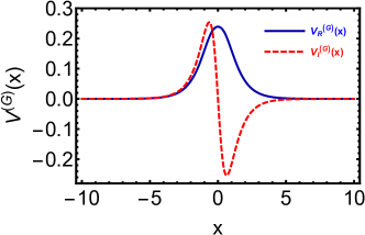
Figure 10: Real part (solid blue line) and imaginary part (red-dashed line) of two soliton potential from the two soliton solution of the Gardner equation for $k_{1}=1.5$, $k_{2}=1.1$, $\alpha_{1}=1$ and $\beta_{1}=1$.

Fig. 10 shows the real and imaginary parts of the two soliton potential from the two soliton solution of the Gardner equation. The shape of this two soliton potential can be altered by changing the values of the solution parameters $k_{1}$ and $k_{2}$.

Finally, we extend the above construction procedure of complex potentials from the periodic solution of the Gardner equation to special dnoidal, cnoidal and superposed elliptic solutions of the Gardner equation, which have been obtained by one of us [46] with $\gamma=6\alpha_{1}$, $\alpha=6\beta_{1}$ and $\delta=1$. For brevity, we present these solutions and the corresponding complex $PT$-invariant potentials in Table 2.

Table 2: Novel type of complex potential for the Gardner equation

Type of	$q(x,t)$	$q(x)$	$V^{(G)}(x)$	Parametric
solutions.				constraints
dnoidal	$A_{1}+B_{1}\times$	$A_{1}+B_{1}\times$	$\Big{[}\alpha_{1}(A_{1}+B_{1}~{}\mbox{dn}(px,m))$	$A_{1}=-\frac{\alpha_{1}}{2\beta_{1}}$
	$\mbox{dn}(\vartheta,m)$	$~{}\mbox{dn}(px,m).$	$-\beta_{1}(A_{1}+B_{1}~{}\mbox{dn}(px,m))^{2}$	$B_{1}^{2}=\frac{p^{2}}{\beta_{1}}$
solution			$-iB_{1}~{}\mbox{m}~{}\sqrt{\beta_{1}}~{}p~{}\mbox{cn}(px,m)$	$v_{1}=$
			$\mbox{sn}(px,m)$]	$(2-m)p^{2}$
				$-\frac{3\alpha_{1}^{2}}{2\beta_{1}}$
cnoidal	$A_{1}+B_{1}\times$	$A_{1}+B_{1}\times$	$\Big{[}\alpha_{1}(A_{1}+B_{1}\sqrt{m}~{}\mbox{cn}(px,m))$	$A_{1}=-\frac{\alpha_{1}}{2\beta_{1}}$
	$\sqrt{m}~{}\mbox{cn}(\vartheta,m)$	$\sqrt{m}~{}\mbox{cn}(px,m).$	$-\beta_{1}(A_{1}+B_{1}\sqrt{m}~{}\mbox{cn}(px,m))^{2}$	$B_{1}^{2}=\frac{p^{2}}{\beta_{1}}$
solution			$-i~{}B_{1}~{}\sqrt{m\beta_{1}}~{}p~{}\mbox{dn}(px,m)$	$v_{1}=$
			$\mbox{sn}(px,m)$]	$(2m-1)p^{2}$
				$-\frac{3\alpha_{1}^{2}}{2\beta_{1}}$
Superposed	$A_{1}+\frac{B_{1}}{2}\times$	$A_{1}+\frac{B_{1}}{2}\times$	$\Bigg{[}\frac{(\alpha_{1}}{2}~{}\Big{(}2A_{1}+B_{1}~{}\mbox{dn}(px,m)$	$A_{1}=-\frac{\alpha_{1}}{2\beta_{1}}$
	$\mbox{dn}(\vartheta,m)+$	$~{}\mbox{dn}(px,m)+$	$+D~{}\mbox{cn}(px,m)\Big{)}-\frac{\beta_{1}}{4}\Big{(}2A_{1}$	$B_{1}^{2}=\frac{p^{2}}{\beta_{1}}$
solution	$\frac{D}{2}\sqrt{m}~{}\mbox{cn}(\vartheta,m)$	$\frac{D}{2}\sqrt{m}~{}\mbox{cn}(px,m)$	$+B_{1}~{}\mbox{dn}(px,m)$	$D=\pm B_{1}$
			$+D~{}\mbox{cn}(px,m)\Big{)}^{2}$	$v_{1}=$
			$-i\frac{\sqrt{\beta_{1}}~{}p~{}\mbox{sn}(px,m)}{2}$	$\frac{(1+m)p^{2}}{2}$
			$\Big{(}B_{1}~{}\mbox{dn}(px,m)$	$-\frac{3\alpha_{1}^{2}}{2\beta_{1}}$
			$+D~{}\mbox{cn}(px,m)\Big{)}\Bigg{]}$

In Table 2, $\vartheta=p(x+\delta_{0}(t))$, where $\delta_{0}(t)$ is given by $(-v_{1}t+x_{0})$ ($x_{0}$ is a constant). We exclude the time dependent part in the third column by choosing the initial time $t_{0}$ such that $\delta_{0}(t_{0})=-v_{1}t_{0}+x_{0}=0$.

It is easily checked that all three potentials presented in Table 2 satisfy $\cal PT$-symmetry.

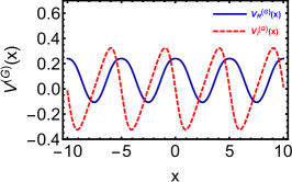
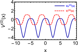
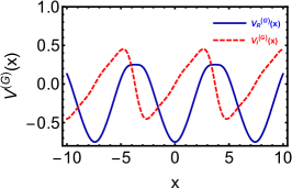
Figure 11: Real part (solid blue line) and imaginary part (red-dashed line) of the elliptic complex potential of the dnoidal (left-panel) potential for $p=0.9$ and $m=0.8$; cnoidal (middle-pannel) potential for $p=1.5$ and $m=0.5$ and superposed (right-panel) potential for $p=1$ and $m=0.5$ respectively. In all the figures $\alpha_{1}=\beta_{1}=1$.

In Fig. 11, we depict the real and the imaginary parts of the dnoidal, cnoidal and superposed potentials from the corresponding solution of the Gardner equation, respectively. All these potentials have robust shape even if we alter the corresponding solution parameters.

6 Conclusion

In this paper, we have constructed a large number of complex potentials including $\cal PT$ -symmetric potentials of the stationary Schrödinger equation from the various interesting soliton and periodic solution of the four fundamental and ubiquitous real NLEEs, namely sG, mKdV, mKdV-sG and Gardner equations, based on their corresponding Lax representation. We have considered several different solutions of those equations namely soliton and periodic soliton solutions and systematically constructed distinct classes of so called Wadati potentials. Remarkably, in majority of cases these potentials turned out to be $\cal PT$-symmetric while in the case of the breather or the periodic breather solutions the corresponding potentials are not $\cal PT$-invariant. We also investigate the robust nature of shape of the complex potentials by altering the corresponding solution parameters. One of the nontrivial issues that we have partially addressed in this paper is whether $\cal PT$-symmetry is spontaneously broken or not in those potentials which are $\cal PT$-invariant. For those cases where the solutions are derived using the IST method one knows for sure that for the solitonic solutions the energy eigenvalues are real and hence $\cal PT$ symmetry is not spontaneously broken. On the other hand, from the IST method one knows that the energy eigenvalues are complex conjugate pair in the case of the complex potentials following from the breather solution. In any case for such complex conjugate eigenvalues the complex potential does not admit $\cal PT$-symmetry. However, we have also obtained potentials by using periodic soliton solutions of these equations. In this case we have no guidance from the IST method. Therefore we have numerically calculated few low lying energy eigenvalues in all these cases and remarkably we found in each and every case of this paper that whenever the complex potential is $\cal PT$-invariant, then the energy eigenvalues turn out to be real and hence $\cal PT$-symmetry is not spontaneously broken. On the otherhand, whenever the complex potential is not $\cal PT$-invariant, we found that the corresponding low lying energy eigenvalues are complex thereby suggesting that in all the $\cal PT$-invariant potentials derived in this way, the $\cal PT$-symmetry is not spontaneously broken. It would be nice if one can rigorously prove this in all such cases.

A salient feature of our above study is that we have constructed complex potentials by starting from real NLEEs. To the best of our knowledge all the identified $\cal PT$ -symmetric potentials are new except for the Scarf-II potential. We have also shown the possible relevance of these $\cal PT$-symmetric potentials (and hence solutions) from the solution of the sG and mKdV-sG systems in the context of the graphene model. Finally, we hope that the various $\cal PT$ and non-$\cal PT$ -symmetric potentials obtained here will shed some light on $\cal PT$ -symmetric quantum mechanics.

References

***

References

- [1] Bender C M, Boettcher S 1998 Phys. Rev. Lett. 80 5243; Bender C M 2005 Contemp. Phys. 46 277.
- [2] El-Ganainy R, Makris K G, Christodoulides D N, Musslimani Z H 2007 Opt. Lett. 32 2632.
- [3] Rüter C E, Markis K G, Ramy El-Ganainy, Christodoulides D N, Segev M, Kip D 2010 Nat. Phys. 6 192–195.
- [4] Peng B, Özdemir S K, Lei F, Monifi F, Gianfreda M, Long G L, Fan S, Nori F, Bender C M, Yang L 2014 Nat. Phys. 5 2927.
- [5] Musslimani Z H, Makris K G, El-Ganainy R, Christodoulides D N 2008 Phys. Rev. Lett. 100 030402.
- [6] Abdullaev F K, Kartashov Y V, Konotop V V, Zezyulin D A 2011 Phys. Rev. A 83 041805(R).
- [7] He Y, Zhu X, Mihalache D, Liu J, Chen Z 2012 Phys. Rev. A 85 013831.
- [8] Moreira F C, Abdullaev F K, Konotop V V, Yulin A V 2012 Phys. Rev. A 86 053815.
- [9] Truong Vu, Y N, D’ Ambroise J, Abdullaev F K, Kevrekidis P G 2015 arXiv:1501.00519v1
- [10] Moreira F C, Konotop V V, Malomed B A 2013 Phys. Rev. A 87 013832.
- [11] Achilleos V, Kevrekidis P G, Frantzeskakis D J, Carretero-Gonzalez R 2013 Phys. Rev. A 86 013808.
- [12] Musslimani Z H, Makris K G, El-Ganainy R, Christodoulides D N, 2008 Phys. Rev. Lett 100, 030402.
- [13] Li H, Shi Z, Jiang X, Zhu X, 2011 Opt. Lett. 36 3290; Musslimani Z H, Makris K G, El-Ganainy R, Christodoulides D N, 2008 J. Phys. A, Math. Theor. 41 244019.
- [14] Hu S, Ma X, Hu W, 2011 Phys. Rev. A 84 043818.
- [15] Hu S, Hu W, 2012 J. Phys. B. At. Mol. Opt. Phys. 45 225401.
- [16] Midya B, Roychoudhury R, 2013 Phy. Rev. A. 87 045803.
- [17] Zezyulin D A, Konotop V V, 2012 Phys.Rev. A 85 043840.
- [18] Avinash Khare, Al-Marzoug S M, Bahlouli H 2012 Phys. Lett. A 376, 2880.
- [19] Honga W P, Jung Y D 2015 Phys. Lett. A 379, 676–679.
- [20] Zhan K, Tian H, Li X, Xu X, Jiao Z, Jia Y 2016 Sci. Rep. 6, 32990.
- [21] Achilleos V, Kevrekidis P G, Frantzeskakis D J, Carretero-González R, 2012 Phys.Rev. A 86 013808; Zezyulin D A, Barashenkov I V, Konotop V V, 2016 Phys. Rev. A 94 063649.
- [22] Wadati M 2008 J. Phys. Soc. Jpn 77 074005.
- [23] Yang J 2014 Opt. Lett. 39 5547.
- [24] Tsoy E N, Allayarov I M, Abdullaev F K 2014 Opt. Lett. 39 4215.
- [25] Yang J, Nixon S 2016 Phys. Lett. A 380 3803.
- [26] Zezyulin D A, Barashenkov I V, Konotop V V 2016 Phys. Rev. A 94 063649.
- [27] Mineev M B, Shmidt V V 1980 Zh. Eksp. Teor. Fiz. 79 893; Rice M, Bishop A R, Krumhansl J A, Trullinger S E 1976 Phys. Rev. Lett. 36 432; Salerno M 1991 Phys. Rev. A 44 5292.
- [28] Lonngren K E 1998 Opt. Quantum Electron. 30 615; Khater A H, El-Kakaawy O H, Callebaut D K 1998 Phys. Scr. 58 545; Ziegler V, Dinkel J, Setzer C, Lonngren K E 2001 Chaos, Solitons Fractals 12 1719; Komatsu T S, Sasa S I 1995 Phys. Rev. E 52 5574.
- [29] Konno K, Kameyama W, Sanuki H 1974 J. Phys. Soc. Jpn. 37 171; Leblond H, Melńikov I V, Mihalache D 2008 Phys. Rev. A 78 043802.
- [30] Ruderman M S, Talipova T, Pelinovsky E 2008 J. Plasma Phys. 74 639; Grimshaw R, Slunyaev A, Pelinovsky E 2010 Chaos 20 013102.
- [31] Meĺnikov I V, Mihalache D, Moldoveanu F, Panoiu, N C 1997 Phys. Rev. A 56 1569; Leblond H, Sanchez F 2003 Phys. Rev. A 67 013804; Meĺnikov I V, Leblond H, Sanchez F, Mihalache D 2004 IEEE J. Sel. Top. Quantum Electron. 10 870; Leblond H, Sazonov S V, Meĺnikov I V, Mihalache D, Sanchez F 2006 IEEE J. Sel. Top. Quantum Electron. 74 063815.
- [32] Barashenkov I V, Zezyulin D A, Konotop V V, 2016 Exactly solvable Wadati potentials in the -symmetric Gross-Pitaevskii equation, in NonHermitian Hamiltonians in Quantum Physics Proc. of the 15 Conf. on Non-Hermitian Hamiltonians in Quantum Physics (Palermo, Italy, 18-23 May 2015) ed Bagarello F, Passante P, Trapani C (Springer International Publishing, Cham, Switzerland) 184 143-155.
- [33] Ho C L, Roy P 2015 EPL, 112 47004.
- [34] R. Rajaraman 1982 Solitons and Instantons North Holland, Amsterdam, The Netherlands.
- [35] Cuevas-Maraver J, Kevrekidis P G, Williams F, eds., 2014 The sine-Gordon model and its applications, Nonlinear systems and complexity, Springer International Publishing, Switzerland.
- [36] Konotop V V, Yang J, Zezyulin D A 2016 Rev. Mod. Phys. 88 035002.
- [37] DelĺAnna L, Martino A D 2009 Phys. Rev. B. 79 045420.
- [38] Ablowitz M J, Segur H 1981 Solitons And Inverse Scattering Transform SIAM, Philadelphia; Caudrey P J, Gibbon J D, Eilbeck J C, Bullough R K 1973 Phys. Rev. Lett. 30 237.
- [39] Cen J, Correa F, Fring A, 2017 arXiv1705.04749.
- [40] Gendenshtein L E 1983 Zh. Eksp. Teor. Fiz. Pis. Red 38 299(Eng. transl. 1983 JETP Lett. 38 35).
- [41] Shi Z, Jiang X, Zhu X, Li H, 2011 Phys. Rev. A 84 053855.
- [42] Fu Z, Liu Shida, Liu Shida 2007 Phys. Scr. 76 15–21.
- [43] Drazin P G, Johnson R S 1989 Solitons: an introduction Cambridge University Press;Kevrekidis P G, Avinash Khare, Saxena A 2003 Phys. Rev. E 68 047701; Kevrekidis P G, Avinash Khare, Saxena A, Herring G 2004 J. Phys. A: Math. Gen. 37 10959.
- [44] Wadati M 1973 J. Phys. Soc. Jpn. 34 1289; Wadati M 1973 J. Phys. Soc. Jpn. 38 681.
- [45] Wazwaz, A M 2009 Partial Differential Equations and Solitary Waves Theory Springer, New York.
- [46] Avinash Khare, Saxena A 2014 J. Maths. Phys. 55 032701.
***