Above and Beyond the Landauer Bound:
Thermodynamics of Modularity

Abstract

Information processing typically occurs via the composition of modular units, such as universal logic gates. The benefit of modular information processing, in contrast to globally integrated information processing, is that complex global computations are more easily and flexibly implemented via a series of simpler, localized information processing operations which only control and change local degrees of freedom. We show that, despite these benefits, there are unavoidable thermodynamic costs to modularity—costs that arise directly from the operation of localized processing and that go beyond Landauer’s dissipation bound for erasing information. Integrated computations can achieve Landauer’s bound, however, when they globally coordinate the control of all of an information reservoir’s degrees of freedom. Unfortunately, global correlations among the information-bearing degrees of freedom are easily lost by modular implementations. This is costly since such correlations are a thermodynamic fuel. We quantify the minimum irretrievable dissipation of modular computations in terms of the difference between the change in global nonequilibrium free energy, which captures these global correlations, and the local (marginal) change in nonequilibrium free energy, which bounds modular work production. This modularity dissipation is proportional to the amount of additional work required to perform the computational task modularly. It has immediate consequences for physically embedded transducers, known as information ratchets. We show how to circumvent modularity dissipation by designing internal ratchet states that capture the global correlations and patterns in the ratchet’s information reservoir. Designed in this way, information ratchets match the optimum thermodynamic efficiency of globally integrated computations. Moreover, for ratchets that extract work from a structured pattern, minimized modularity dissipation means their hidden states must be predictive of their input and, for ratchets that generate a structured pattern, this means that hidden states are retrodictive.

I Introduction

Physically embedded information processing operates via thermodynamic transformations of the supporting material substrate. The thermodynamics is best exemplified by Landauer’s principle: erasing one bit of stored information at temperature $T$ must be accompanied by the dissipation of at least $k_{\text{B}}T\ln{2}$ amount of heat [1] into the substrate. While the Landauer cost is only time-asymptotic and not yet the most significant energy demand in everyday computations—in our cell phones, tablets, laptops, and cloud computing—there is a clear trend and desire to increase thermodynamic efficiency. Digital technology is expected, for example, to reach the vicinity of the Landauer cost in the near future; a trend accelerating with now-promising quantum computers. This seeming inevitability forces us to ask if the Landauer bound can be achieved for more complex information processing tasks than writing or erasing a single bit of information.

In today’s massive computational tasks, in which vast arrays of bits are processed in sequence and in parallel, a task is often broken into modular components to add flexibility and comprehensibility to hardware and software design. This holds far beyond the arenas of today’s digital computing. Rather than tailoring processors to do only the task specified, there is great benefit in modularly deploying elementary, but universal functional components—e.g., NAND, NOR, and perhaps Fredkin [2] logic gates, biological neurons [3], or similar units appropriate to other domains [4]—that can be linked together into circuits which perform any functional operation. This leads naturally to hierarchical design, perhaps across many organizational levels. In these ways, the principle of modularity reduces the challenges of designing, monitoring, and diagnosing efficient processing considerably [5, 6]. Designing each modular component of a complex computation to be efficient is vastly simpler than designing and optimizing the whole. Even biological evolution seems to have commandeered prior innovations, remapping and reconnecting modular functional units to form new organizations and new organisms of increasing survivability [7].

There is, however, a potential thermodynamic cost to modular information processing. For concreteness, recall the stochastic computing paradigm in which an input (a sequence of symbols) is sampled from a given probability distribution and the symbols are correlated to each other. In this setting, a modularly designed computation processes only the local component of the input, ignoring the latter’s global structure. This inherent locality necessarily leads to irretrievable loss of the global correlations during computing. Since such correlations are a thermal resource [8, 9], their loss implies an energy cost—a thermodynamic modularity dissipation. Employing stochastic thermodynamics and information theory, we show how modularity dissipation arises by deriving an exact expression for dissipation in a generic localized information processing operation. We emphasize that this dissipation is above and beyond the Landauer bound for losses in the operation of single logical gates. It arises solely from the modular architecture of complex computations. One immediate consequence is that the additional dissipation requires investing additional work to drive computation forward.

In general, to minimize work invested in performing a computation, we must leverage the global correlations in a system’s environment. Globally integrated computations can achieve the minimum dissipation by simultaneous control of the whole system, manipulating the joint system-environment Hamiltonian to follow the desired joint distribution. Not only is this level of control difficult to implement physically, but designing the required protocol poses a considerable computational challenge in itself, with so many degrees of freedom and a potentially complex state space. Genetic algorithm methods have been proposed, though, for approximating the optimum [10]. Tellingly, they can find unusual solutions that break conventional symmetries and take advantage of the correlations between the many different components of the entire system [11, 12]. However, as we will show, it is possible to rationally design local information processors that, by accounting for these correlations, minimized modularity dissipation.

The following shows how to design optimal modular computational schemes such that useful global correlations are not lost, but stored in the structure of the computing mechanism. Since the global correlations are not lost in these optimal schemes, the net processing can be thermodynamically reversible (dissipationless). Utilizing the tools of information theory and computational mechanics—Shannon information measures and optimal hidden Markov generators—we identify the informational system structures that can mitigate and even nullify the potential thermodynamic cost of modular computation.

A brief tour of our main results will help orient the reader. It can even serve as a complete, but approximate description for the approach and technical details, should this be sufficient for the reader’s interests.

Section II considers the thermodynamics of a composite information reservoir, in which only a subsystem is amenable to external control. In effect, this is our model of a localized thermodynamic operation. We assume that the information reservoir is coupled to an ideal heat bath, as a source of randomness and energy. Thus, external control of the information reservoir yields random Markovian dynamics over the informational states, heat flows into the heat bath, and work investment from the controller. Statistical correlations may exist between the controlled and uncontrolled subsystems, either due to initial or boundary conditions or due to an operation’s history.

To highlight the information-theoretic origin of the dissipation and to minimize the energetic aspects, we assume that the informational states have equal internal (free) energies. Appealing to stochastic thermodynamics and information theory, we then show that the minimum irretrievable modularity dissipation over the duration of an operation due to the locality of control is proportional to the reduction in mutual information between the controlled and uncontrolled subsystems; see Eq. (5). We deliberately refer to “operation” here instead of “computation” since the result holds whether the desired task is interpreted as computation or not. The result holds so long as free-energy uniformity is satisfied at all times, a condition natural in computation and other information processing settings.

Section III applies this analysis to information engines, an active subfield within the thermodynamics of computation in which information effectively acts as the fuel for driving physically embedded information processing [13, 14, 15, 16, 8]. The particular implementations of interest—information ratchets—process an input symbol string by interacting with each symbol in order, sequentially transforming it into an output symbol string, as shown in Fig. 3. This kind of information transduction [17, 14] is information processing in a very general sense: with a properly designed finite-state control, the devices can implement a universal Turing machine [18]. Since information engines rely on localized information processing, reading in and manipulating one symbol at a time in their original design [13], the measure of irretrievable dissipation applies directly. The exact expression for the modularity dissipation is given in Eq. (13).

Sections IV and V specialize information transducers further to the cases of pattern extractors and pattern generators. Section IV’s pattern extractors use structure in their environment to produce work and pattern generators use stored work to create structure from an unstructured environment. The irreversible relaxation of correlations in information transduction can then be curbed by intelligently designing these computational processes. While there are not yet general principles for designing implementations for arbitrary computations, the measure of modularity dissipation that we develop in the following shows how to construct energy-efficient extractors and generators. For example, efficient extractors consume complex patterns and turn them into sequences of independent and identically distributed (IID) symbols.

We show that extractor transducers whose states are predictive of their inputs are optimal, with zero minimal modularity dissipation. This makes immediate intuitive sense since, by design, such transducers can anticipate the next input and adapt accordingly. This observation also emphasizes the principle that thermodynamic agents should requisitely match the structural complexity of their environment to leverage those informational correlations as a thermodynamic fuel [16]. We illustrate this result in the case of the Golden Mean pattern in Fig. 4.

Conversely, Section V shows that when generating patterns from unstructured IID inputs, transducers whose states are retrodictive of their output are most efficient—i.e., have minimal modularity dissipation. This is also intuitively appealing in that pattern generation may be viewed as the time reversal of pattern extraction. Since predictive transducers are efficient for pattern extraction, retrodictive transducers are expected to be efficient pattern generators; see Fig. 6. This also allows one to appreciate that pattern generators previously thought to be asymptotically efficient are actually quite dissipative [19]. Taken altogether, these results provide guideposts for designing efficient, modular, and complex information processors—guideposts that go substantially beyond Landauer’s principle for localized processing.

II Global versus Localized Processing

If a physical system, denote it $\mathcal{Z}$, stores information as it behaves, it acts as an information reservoir. Then, a wide range of physically-embedded computational processes can be achieved by connecting $\mathcal{Z}$ to an ideal heat bath at temperature $T$ and externally controlling the system’s physical parameters, its Hamiltonian. Coupling with the heat bath allows for physical phase-space compression and expansion, which are necessary for useful computations and which account for the work investment and heat dissipation dictated by Landauer’s bound. However, the bound is only achievable when the external control is precisely designed to harness the changes in phase-space. This may not be possible for modular computations. The modularity here implies that control is localized and potentially ignorant of global correlations in $\mathcal{Z}$. This leads to uncontrolled changes in phase-space.

Most computational processes unfold via a sequence of local operations that update only a portion of the system’s informational state. A single step in such a process can be conveniently described by breaking the whole informational system $\mathcal{Z}$ into two constituents: the informational states $\mathcal{Z}^{\text{int}}$ that are controlled and evolving and the informational states $\mathcal{Z}^{\text{stat}}$ that are not part of the local operation on $\mathcal{Z}^{\text{int}}$. We call $\mathcal{Z}^{\text{int}}$ the interacting subsystem and $\mathcal{Z}^{\text{stat}}$ the stationary subsystem. As shown in Fig. 1, the dynamic over the joint state space $\mathcal{Z}=\mathcal{Z}^{\text{int}}\otimes\mathcal{Z}^{\text{stat}}$ is the product of the identity over the stationary subsystem and a local Markov channel over the interacting subsystem. The informational states of the noninteracting stationary subsystem $\mathcal{Z}^{\text{stat}}$ are fixed over the immediate computational task, since this information should be preserved for use in later computational steps.

Such classical computations are described by a global Markov channel over the joint state space:

$$M^{\text{global}}_{z^{\text{i}}_{t},z^{\text{s}}_{t}\rightarrow z^{\text{i}}_{t+\tau},z^{\text{s}}_{t+\tau}}$$

$$\quad=\Pr(Z^{\text{i}}_{t+\tau}\!=\!z^{\text{i}}_{t+\tau},Z^{\text{s}}_{t+\tau}\!=\!z^{\text{s}}_{t+\tau}|Z^{\text{i}}_{t}\!=\!z^{\text{i}}_{t},Z^{\text{s}}_{t}\!=\!z^{\text{s}}_{t}),$$ (1)

where $Z_{t}=Z^{\text{i}}_{t}\otimes Z^{\text{s}}_{t}$ and $Z_{t+\tau}=Z^{\text{i}}_{t+\tau}\otimes Z^{\text{s}}_{t+\tau}$ are the random variables for the informational state of the joint system before and after the computation, with $Z^{\text{i}}$ describing the $\mathcal{Z}^{\text{int}}$ subspace and $Z^{\text{s}}$ the $\mathcal{Z}^{\text{stat}}$ subspace, respectively. (Lowercase variables denote values their associated random variables realize.) The righthand side of Eq. (1) gives the transition probability over the time interval $(t,t+\tau)$ from joint state $(z^{\text{i}}_{t},z^{\text{s}}_{t})$ to state $(z^{\text{i}}_{t+\tau},z^{\text{s}}_{t+\tau})$. The fact that $\mathcal{Z}^{\text{stat}}$ is fixed means that the global dynamic can be expressed as the product of a local Markov computation on $\mathcal{Z}^{\text{int}}$ with the identity over $\mathcal{Z}^{\text{stat}}$:

$$M^{\text{global}}_{(z^{\text{i}}_{t},z^{\text{s}}_{t})\rightarrow(z^{\text{i}}_{t+\tau},z^{\text{s}}_{t+\tau})}=M^{\text{local}}_{z^{\text{i}}_{t}\rightarrow z^{\text{i}}_{t+\tau}}\delta_{z^{\text{s}}_{t},z^{\text{s}}_{t+\tau}}~{},$$ (2)

where the local Markov computation is the conditional marginal distribution:

$$M^{\text{local}}_{z^{\text{i}}_{t}\rightarrow z^{\text{i}}_{t+\tau}}=\Pr(Z^{\text{i}}_{t+\tau}=z^{\text{i}}_{t+\tau}|Z^{\text{i}}_{t}=z^{\text{i}}_{t})~{}.$$ (3)

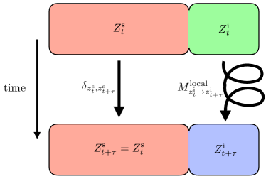
Figure 1: Local computations operate on only a subset $\mathcal{Z}^{\text{int}}$ of the entire information reservoir $\mathcal{Z}=\mathcal{Z}^{\text{int}}\otimes\mathcal{Z}^{\text{stat}}$. The Markov channel that describes the global dynamic is the product of a local operation with the identity operation: $M^{\text{global}}_{(z^{\text{i}}_{t},z^{\text{s}}_{t})\rightarrow(z^{\text{i}}_{t+\tau},z^{\text{s}}_{t+\tau})}=M^{\text{local}}_{z^{\text{i}}_{t}\rightarrow z^{\text{i}}_{t+\tau}}\delta_{z^{\text{s}}_{t},z^{\text{s}}_{t+\tau}}$, such that the stationary noninteracting portion $Z^{\text{s}}$ of the information reservoir remains invariant, but the interacting portion $Z^{\text{i}}$ changes.

When the processor is in contact with a heat bath at temperature $T$, the average entropy production $\langle\Sigma_{t\rightarrow t+\tau}\rangle$ of the universe over the time interval $(t,t+\tau)$ can be expressed in terms of the work done minus the change in nonequilibrium free energy $F^{\text{neq}}$:

$$\langle\Sigma_{t\rightarrow t+\tau}\rangle=\frac{\langle W_{t\rightarrow t+\tau}\rangle-(F^{\text{neq}}_{t+\tau}-F^{\text{neq}}_{t})}{T}~{}.$$

In turn, the nonequilibrium free energy $F^{\text{neq}}_{t}$ at any time $t$ can be expressed as the weighted average of the internal (free) energy $U_{z}$ of the joint informational states minus the uncertainty in those states:

$$F^{\text{neq}}_{t} =\sum_{z}\Pr(Z=z)U_{z}-k_{\text{B}}T\ln 2\operatorname{H}[Z_{t}]~{}.$$

Here, $\operatorname{H}[Z]$ is the Shannon information of the random variable $Z$ that realizes the state of the joint system $\mathcal{Z}$ [20]. When the information bearing degrees of freedom support an information reservoir, where all states $z$ and $z^{\prime}$ have the same internal energy $U_{z}=U_{z^{\prime}}$, the entropy production reduces to the work minus a change in Shannon information of the information-bearing degrees of freedom:

$$\langle\Sigma_{t\rightarrow t+\tau}\rangle=\frac{\langle W_{t\rightarrow t+\tau}\rangle}{T}\!+\!k_{\text{B}}\ln 2(\operatorname{H}[Z_{t+\tau}]\!-\!\operatorname{H}[Z_{t}])~{}.$$ (4)

Essentially, this is an expression of a generalized Landauer Principle: entropy increase guarantees that work production is bounded by the change in Shannon entropy of the informational variables [1].

In particular, for a globally integrated quasistatic operation, where all degrees of freedom are controlled simultaneously as discussed in App. A, there is zero entropy production. And, the globally integrated work done on the system achieves the theoretical minimum:

$$\langle W_{t\rightarrow t+\tau}^{\text{global}}\rangle_{\text{min}}=-k_{\text{B}}T\ln 2(\operatorname{H}[Z_{t+\tau}]-\operatorname{H}[Z_{t}])~{}.$$

The process is reversible since the change in system Shannon entropy balances the change in the reservoir’s physical entropy due to heat dissipation. (Since the internal energy is uniform, the system cannot store the work and must dissipate it as heat to the surrounding environment.) This may not be the case for a generic modular operation.

There are two consequences of the locality of control. First, since $Z^{\text{s}}$ is kept fixed—that is, $Z^{\text{s}}_{t}=Z^{\text{s}}_{t+\tau}$—the change in uncertainty $\operatorname{H}[Z^{\text{i}}_{t+\tau},Z^{\text{s}}_{t+\tau}]-\operatorname{H}[Z^{\text{i}}_{t},Z^{\text{s}}_{t}]$ of the joint informational variables during the operation, which is the second term in lefthand side of Eq. (4), simplifies to:

$$\operatorname{H}[Z_{t+\tau}]-\operatorname{H}[Z_{t}]=\operatorname{H}[Z^{\text{i}}_{t+\tau},Z^{\text{s}}_{t}]-\operatorname{H}[Z^{\text{i}}_{t},Z^{\text{s}}_{t}]~{}.$$

Second, since we operate locally on $Z^{\text{i}}$, with no knowledge of $Z^{\text{s}}$, then the required work is bounded by the generalized Landauer Principle corresponding to the marginal distribution over $Z^{\text{i}}$; see Eq. (2). In other words, in absence of any control over the noninteracting subsystem $Z^{\text{s}}$, which remains stationary over the local computation on $Z^{\text{i}}$, the minimum work performed on $Z^{\text{i}}$ is given by:

$$\langle W_{t\rightarrow t+\tau}\rangle \geq\langle W^{\text{local}}_{t\rightarrow t+\tau}\rangle_{\text{min}}$$

$$=k_{\text{B}}T\ln 2(\operatorname{H}[Z^{\text{i}}_{t}]-H[Z^{\text{i}}_{t+\tau})~{}.$$

This bound is achievable through a sequence of quasistatic and instantaneous protocols, described in App. A.

Combining the last two relations with the expression for entropy production in Eq. (4) gives the modularity dissipation $\Sigma^{\text{mod}}$, which is the minimum irretrievable dissipation of a modular computation that comes from local interactions:

$$\frac{\langle\Sigma^{\text{mod}}_{t\rightarrow t+\tau}\rangle_{\text{min}}}{k_{\text{B}}\ln 2} =\frac{\langle W^{\text{local}}_{t\rightarrow t+\tau}\rangle_{\text{min}}}{k_{B}T\ln 2}+\operatorname{H}[Z^{\text{i}}_{t+\tau},Z^{\text{s}}_{t}]-\operatorname{H}[Z^{\text{i}}_{t},Z^{\text{s}}_{t}]$$

$$=\operatorname{I}[Z^{\text{i}}_{t};Z^{\text{s}}_{t}]-I[Z^{\text{i}}_{t+\tau};Z^{\text{s}}_{t}]~{},$$ (5)

where $\operatorname{I}[X;Y]$ is the mutual information between the random variables $X$ and $Y$.

This is our central result: there is a thermodynamic cost above and beyond the Landauer bound for modular operations. It is a thermodynamic cost arising from a computation’s implementation architecture. Specifically, the minimum entropy production is proportional to the minimum additional work that must be done to execute a computation modularly:

$$\langle W^{\text{local}}_{t\rightarrow t+\tau}\rangle_{\text{min}}-\langle W^{\text{global}}_{t\rightarrow t+\tau}\rangle_{\text{min}}=T\langle\Sigma^{\text{mod}}_{t\rightarrow t+\tau}\rangle_{\text{min}}~{}.$$

The following draws out the implications.

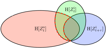
Figure 2: Information diagram for a local computation: Information atoms of the noninteracting subsystem $\operatorname{H}[Z^{\text{s}}_{t}]$ (red ellipse), the interacting subsystem before the computation $\operatorname{H}[Z^{\text{i}}_{t}]$ (green circle), and the interacting subsystem after the computation $\operatorname{H}[Z^{\text{i}}_{t+\tau}]$ (blue circle). The initial state of the interacting subsystem shields the final state from the noninteracting subsystem; graphically the blue and red ellipses only overlap within the green ellipse. The modularity dissipation is proportional to the difference between information atoms $\operatorname{I}[Z^{\text{i}}_{t};Z^{\text{s}}_{t}]$ and $\operatorname{I}[Z^{\text{i}}_{t+\tau};Z^{\text{s}}_{t}]$. Due to statistical shielding, it simplifies to the information atom $\operatorname{I}[Z^{\text{i}}_{t};Z^{\text{s}}_{t}|Z^{\text{i}}_{t+\tau}]$, highlighted by a red dashed outline.

Using the fact that the local operation $M^{\text{local}}$ ignores $Z^{\text{s}}$, we see that the joint distribution over all three variables $Z^{\text{i}}_{t},Z^{\text{s}}_{t},$ and $Z^{\text{i}}_{t+\tau}$ can be simplified to:

$$\Pr(Z^{\text{i}}_{t+\tau} =z^{\text{i}}_{t+\tau},Z^{\text{i}}_{t}=z^{\text{i}}_{t},Z^{\text{s}}_{t}=z^{\text{s}}_{t})$$

$$=\Pr(Z^{\text{i}}_{t+\tau}=z^{\text{i}}_{t+\tau}|Z^{\text{i}}_{t}=z^{\text{i}}_{t})\Pr(Z^{\text{i}}_{t}=z^{\text{i}}_{t},Z^{\text{s}}_{t}=z^{\text{s}}_{t})~{}.$$

Thus, $Z^{\text{i}}_{t}$ shields $Z^{\text{i}}_{t+\tau}$ from $Z^{\text{s}}_{t}$. A consequence is that the mutual information between $Z^{\text{i}}_{t+\tau}$ and $Z^{\text{s}}_{t}$ conditioned on $Z^{\text{i}}_{t}$ vanishes. This is shown in Fig. 2 via an information diagram. Figure 2 also shows that the modularity dissipation, highlighted by a dashed red outline, can be re-expressed as the mutual information between the noninteracting stationary system $Z^{\text{s}}$ and the interacting system $Z^{\text{i}}$ before the computation that is not shared with $Z^{\text{i}}$ after the computation:

$$\langle\Sigma^{\text{mod}}_{t\rightarrow t+\tau}\rangle_{\text{min}}=k_{\text{B}}\ln 2\operatorname{I}[Z^{\text{i}}_{t};Z^{\text{s}}_{t}|Z^{\text{i}}_{t+\tau}]~{}.$$ (6)

This is our second main result. The conditional mutual information on the right bounds how much entropy is produced when performing a local computation. It quantifies the irreversibility of information processing.

We close this section by noting that Eq. (5)’s bound is analogous to the expression for the minimum work required for data representation, with $Z^{\text{i}}_{t}$ being the work medium, $Z^{\text{i}}_{t+\tau}$ the work extraction device, and $Z^{\text{s}}_{t}$ the data representation device [21].

The following unpacks the implications of Eqs. (5) and (6) for information transducers—information processing architectures in which the processor sequentially takes one input symbol at a time and performs localized computation on it, much as a Turing machine operates.

III Information Transducers: Localized processors

Information ratchets [22, 14] are thermodynamic implementations of information transducers [17] that sequentially transform an input symbol string, described by the chain of random variables $Y_{0:\infty}=Y_{0}Y_{1}Y_{2},\ldots$, into an output symbol string, described by the chain of random variables $Y^{\prime}_{0:\infty}=Y^{\prime}_{0}Y^{\prime}_{1}Y^{\prime}_{2},\ldots$. The ratchet traverses the input symbol string unidirectionally, processing each symbol in turn to yield the output sequence. As shown in Fig. 3, at time $t=N\tau$ the information reservoir is described by the joint distribution over the ratchet state $X_{N}$ and the symbol string $\mathbf{Y}_{N}=Y_{0:N}^{\prime}Y_{N:\infty}$, the concatenation of the first $N$ symbols of the output string and the remaining symbols of the input string. (This differs slightly from previous treatments [8] in which only the symbol string is the information reservoir. The information processing and energetics are the same, however.) Including the ratchet state in present definition of the information reservoir allows us to directly determine the modularity dissipation of information transduction.

Going from time $t=N\tau$ to $t+\tau=(N+1)\tau$ preserves the state of the current output history $Y_{0:N}^{\prime}$ and the input future, excluding the $N$th symbol $Y_{N+1:\infty}$, while changing the $N$th input symbol $Y_{N}$ to the $N$th output symbol $Y_{N}^{\prime}$ and the ratchet from its current state $X_{N}$ to its next $X_{N+1}$. In terms of the previous section, this means the noninteracting stationary subsystem $\mathcal{Z}^{\text{stat}}$ is the entire semi-infinite symbol string without the $N$th symbol:

$$Z^{\text{s}}_{t}=(Y_{N+1:\infty},Y^{\prime}_{0:N})~{}.$$ (7)

The ratchet and the $N$th symbol constitute the interacting subsystem $\mathcal{Z}^{\text{int}}$ so that, over the time interval $(t,t+\tau)$, only two variables change:

$$Z^{\text{i}}_{t}=(X_{N},Y_{N})$$ (8)

and

$$Z^{\text{i}}_{t+\tau}=(X_{N+1},Y_{N}^{\prime})~{}.$$ (9)

Despite the fact that only a small portion of the system changes on each time step, the physical device is able to perform a wide variety of physical and logical operations. Ignoring the probabilistic processing aspects, Turing showed that a properly designed (very) finite-state transducer can compute any input-output mapping [23] . Such machines, even those with as few as two internal states and a sufficiently large symbol alphabet [25] or with as few as a dozen states but operating on a binary-symbol strings, are universal in that sense [26].

Information ratchets—physically embedded, probabilistic Turing machines—are able to facilitate energy transfer between a thermal reservoir at temperature $T$ and a work reservoir by processing information in symbol strings. In particular, they can function as an eraser by using work to create structure in the output string [13, 14] or act as an engine by using the structure in the input to turn thermal energy into useful work energy [14]. They are also capable of much more, including detecting, adapting to, and synchronizing to environment correlations [27, 16] and correcting errors [8].

Information transducers are a novel form of information processor from a different perspective, that of communication theory’s channels [17]. They are memoryful channels that map input stochastic processes to output processes using internal states which allow them to store information about the past of both the input and the output. With sufficient hidden states, as just noted from the view of computation theory, information transducers are Turing complete and so able to perform any computation on the information reservoir [28]. Similarly, the physical steps that implement a transducer as an information ratchet involve a series of modular local computations.

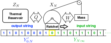
Figure 3: Information ratchet consists of three interacting reservoirs—work, heat, and information. The work reservoir is depicted as gravitational mass suspended by a pulley. The thermal reservoir keeps the entire system thermalized to temperature $T$. At time $N\tau$ the information reservoir consists of (i) a string of symbols $\mathbf{Y}_{N}=Y^{\prime}_{0}Y^{\prime}_{1}\ldots Y^{\prime}_{N-1}Y_{N}Y_{N+1}\ldots$, each cell storing an element from the same alphabet $\mathcal{Y}$ and (ii) the ratchet’s internal state $X_{N}$. The ratchet moves unidirectionally along the string, exchanging energy between the heat and the work reservoirs. The ratchet reads the value of a single cell (highlighted in yellow) at a given time from the input string (green, right), interacts with it, and writes a symbol to the cell in the output string (blue, left) of the information reservoir. Overall, the ratchet transduces the input string $Y_{0:\infty}=Y_{0}Y_{1}\ldots$ into an output string $Y^{\prime}_{0:\infty}=Y^{\prime}_{0}Y^{\prime}_{1}\ldots$. (Reprinted from Ref. [14] with permission.)

The ratchet operates by interacting with one symbol at a time in sequence, as shown in Fig. 3. The $N$th symbol, highlighted in yellow to indicate that it is the interacting symbol, is changed from the input $Y_{N}$ to output $Y^{\prime}_{N}$ over time interval $(N\tau,(N+1)\tau)$. The ratchet and interaction symbol change together according to the local Markov channel over the ratchet-symbol state space:

$$M^{\text{local}}_{(x,y)\rightarrow(x^{\prime},y^{\prime})}=\Pr(X_{N+1}\!=\!x^{\prime},Y_{N}^{\prime}\!=\!y^{\prime}|X_{N}\!=\!x,Y_{N}\!=\!y).$$

This determines how the ratchet transduces inputs to outputs [14].

Each of these localized operations keeps the remaining noninteracting symbols in the information reservoir fixed. If the ratchet only has energetic control of the degrees of freedom it manipulates, then, as discussed in the previous section and App. A, the ratchet’s work production in the $N$th time step is bounded by the change in uncertainty of the ratchet state and interaction symbol:

$$\langle W^{\text{local}}_{N}\rangle_{\text{min}}\!=\!k_{\text{B}}T\ln 2(\operatorname{H}[X_{N},Y_{N}]\!-\!\operatorname{H}[X_{N+1},Y^{\prime}_{N}]).$$ (10)

This bound has been recognized in previous investigations of information ratchets [13, 29]. Here, we make a key, but important and compatible observation: If we relax the condition of local control of energies to allow for global control of all symbols simultaneously, then it is possible to extract more work.

That is, foregoing localized operations—abandoning modularity—allows for (and acknowledges the possibility of) globally integrated interactions. Then, we can account for the change in Shannon information of the information reservoir—the ratchet and the entire symbol string. This yields a looser upper bound on work production that holds for both modular and globally integrated information processing. Assuming that all information reservoir configurations have the same free energies, the change in the nonequilibrium free energy during one step of a ratchet’s computation is proportional to the global change in Shannon entropy:

$$\Delta F^{\text{neq}}_{N\tau\rightarrow(N+t)\tau}\!=\!k_{\text{B}}T\ln 2(\operatorname{H}[X_{N},\mathbf{Y}_{N}]\!-\!\operatorname{H}[X_{N+1},\mathbf{Y}_{N+1}]).$$

Recalling the definition of entropy production $\langle\Sigma\rangle=\langle W\rangle-\Delta F^{\text{neq}}$ reminds us that for entropy to increase, the minimum work investment must match the change in free energy:

$$\langle W^{\text{global}}_{N}\rangle_{\text{min}}$$

$$\quad=k_{\text{B}}T\ln 2(\operatorname{H}[X_{N},\mathbf{Y}_{N}]-\operatorname{H}[X_{N+1},\mathbf{Y}_{N+1}])~{}.$$ (11)

This is the work production that can be achieved through globally integrated quasistatic information processing. And, in turn, it can be used to bound the asymptotic work production in terms of the entropy rates of the input and output processes [14]:

$$\lim_{N\rightarrow\infty}\langle W_{N}\rangle\geq k_{\text{B}}T\ln 2(h_{\mu}-h_{\mu}^{\prime})~{}.$$ (12)

This is known as the Information Processing Second Law (IPSL).

Reference [16] already showed that this bound is not necessarily achievable by information ratchets. This is due to ratchets operating locally. The local bound on work production of modular implementations in Eq. (10) is less than or equal to the global bound on integrated implementations in Eq. (11), since the local bound ignores correlations between the interacting system $\mathcal{Z}^{\text{int}}$ and noninteracting elements of the symbol string in $\mathcal{Z}^{\text{stat}}$. Critically, though, if we design the ratchet such that its states store the relevant correlations in the symbol string, then we can achieve the global bounds. This was hinted at in the fact that the gap between the work done by a ratchet and the global bound can be closed by designing a ratchet that matches the input process’ structure [8]. However, comparing the two bounds now allows us to be more precise.

The difference between the two bounds represents the amount of additional work that could have been performed by a ratchet, if it was not modular and limited to local interactions. If the computational device is globally integrated, with full access to all correlations between the information bearing degrees of freedom, then all of the nonequilibrium free energy can be converted to work, zeroing out the entropy production. Thus, the minimum entropy production for a modular transducer (or information ratchet) at the $N$th time step can be expressed in terms of the difference between Eq. (10) and the entropic bounds in Eq. (11):

$$\frac{\langle\Sigma^{\text{mod}}_{N}\rangle_{\text{min}}}{k_{\text{B}}\ln 2} =\frac{\langle W^{\text{local}}_{N}\rangle_{\text{min}}-\Delta F^{\text{neq}}_{N\tau\rightarrow(N+1)\tau}}{k_{B}T\ln 2}$$ (13)

$$=\operatorname{I}[Y_{N+1:\infty},Y^{\prime}_{0:N};X_{N},Y_{N}]$$

$$\qquad-\operatorname{I}[Y_{N+1:\infty},Y^{\prime}_{0:N};X_{N+1},Y^{\prime}_{N}]$$

$$=\operatorname{I}[Y_{N+1:\infty},Y^{\prime}_{0:N};X_{N},Y_{N}|X_{N+1},Y^{\prime}_{N}]~{}.$$ (14)

This can also be derived directly by substituting our interacting variables $(X_{N},Y_{N})=Z^{\text{i}}_{t}$ and $(X_{N+1},Y^{\prime}_{N})=Z^{\text{i}}_{t+\tau}$ and stationary variables $(Y_{N+1:\infty},Y^{\prime}_{0:N})=Z^{\text{s}}$ into the expression for the modularity dissipation in Eqs. (5) and (6) in Sec. II. Even if the energy levels are controlled so slowly that entropic bounds are reached, Eq. (14) quantifies the amount of lost correlations that cannot be recovered. And, this leads to the entropy production and irreversibility of the transducing ratchet. This has immediate consequences that limit the most thermodynamically efficient information processors.

Figure 4: Multiple ways to transform the Golden Mean Process input, whose $\epsilon$-machine generator is shown in the far left box, into a sequence of uncorrelated symbols. The $\epsilon$-machine is a Mealy hidden Markov model that produces outputs along the edges, with $y:p$ denoting that the edge emits symbol $y$ and is taken with probability $p$. (Top row) Ratchet whose internal states match the $\epsilon$-machine states and so it is able to minimize dissipation—$\langle\Sigma^{\text{ext}}_{\infty}\rangle_{\text{min}}=0$—by making transitions such that the ratchet’s states are synchronized to the $\epsilon$-machine’s states. The transducer representation to the left shows how the states remain synchronized: its edges are labeled $y^{\prime}|y:p$, which means that if the input was $y$, then with probability $p$ the edge is taken and it outputs $y^{\prime}$. The joint Markov representation on the right depicts the corresponding physical dynamic over the joint state space of the ratchet and the interaction symbol. The label $p$ along an edge from the state $x\otimes y$ to $x^{\prime}\otimes y^{\prime}$ specifies the probability of transitioning between those states according to the local Markov channel $M^{\text{local}}_{(x,y)\rightarrow(x^{\prime},y^{\prime})}=p$. (Bottom row) In contrast to the efficient predictive ratchet, the memoryless ratchet shown is inefficient, since it’s memory cannot store the predictive information within the input $\epsilon$-machine, much less synchronize to it.

While previous bounds, such as the IPSL, demonstrated that information in the symbol string can be used as a thermal fuel [13, 14]—leveraging structure in the inputs symbols to turn thermal energy into useful work—they largely ignore the structure of information ratchet states $X_{N}$. The transducer’s hidden states, which can naturally store information about the past, are critical to taking advantage of structured inputs. Until now, we only used informational bounds to predict transient costs to information processing [19, 27]. With the expression for the modularity dissipation of information ratchets in Eq. (14), however, we now have bounds that apply to the ratchet’s asymptotic functioning. In short, this provides the key tool for designing thermodynamically efficient transducers. We will now show that it has immediate implications for pattern generation and pattern extraction.

IV Predictive Extractors

A pattern extractor is a transducer that takes in a structured process $\Pr(Y_{0:\infty})$, with correlations among the symbols, and maps it to a series of independent identically distributed (IID), uncorrelated output symbols. An output symbol can be distributed however we wish individually, but each must be distributed with an identical distribution and independently from all others. The result is that the joint distribution of the output process symbols is the product of the individual marginals:

$$\Pr(Y_{0:\infty}^{\prime})=\prod_{i=0}^{\infty}\Pr(Y_{i}^{\prime})~{}.$$ (15)

If implemented efficiently, this device can use temporal correlations in the input as a thermal resource to produce work. The modularity dissipation of an extractor $\langle\Sigma_{N}^{\text{ext}}\rangle_{\text{min}}$ can be simplified by noting that the output symbols are uncorrelated with any other variable and, thus, fall out of the mutual information terms:

$$\frac{\langle\Sigma_{N}^{\text{ext}}\rangle_{\text{min}}}{k_{B}\ln 2}=\operatorname{I}[Y_{N+1:\infty};X_{N},Y_{N}]-\operatorname{I}[Y_{N+1:\infty};X_{N+1}]~{}.$$

Minimizing this irreversibility, as shown in App. B, leads directly to a fascinating conclusion that relates thermodynamics to prediction: the states of maximally thermodynamically efficient extractors are optimally predictive of the input process.

To take full advantage of the temporal structure of an input process, the ratchet’s states $X_{N}$ must be able to predict the future of the input $Y_{N:\infty}$ from the input past $Y_{0:N}$. Thus, the ratchet shields the input past from the output future such that there is no information shared between the past and future which is not captured by the ratchet’s states:

$$\operatorname{I}[Y_{N:\infty};Y_{0:N}|X_{N}]=0~{}.$$ (16)

Additionally, transducers cannot anticipate the future of the inputs beyond their correlations with past inputs [17]. This means that there is no information shared between the ratchet and the input future when conditioned on the input past:

$$\operatorname{I}[Y_{N:\infty};X_{N}|Y_{0:N}]=0~{}.$$ (17)

Together, Eqs. (16) and (17) are equivalent to both the state $X_{N}$ being predictive and the modularity dissipation vanishing $\langle\Sigma_{N}^{\text{ext}}\rangle_{\text{min}}=0$. The efficiency of predictive ratchets suggests that predictive generators, such as the $\epsilon$-machine [30], are useful in designing efficient information engines that can leverage temporal structure in an environment.

For example, consider an input string that is structured according to the Golden Mean Process, which consists of binary strings in which $1$’s always occur in isolation, surrounded by $0$’s. Figure 4 gives two examples of ratchets, described by different local Markov channels $M^{\text{local}}_{(x,y)\rightarrow(x^{\prime},y^{\prime})}$, that each map the Golden Mean Process to a biased coin. The input process’ $\epsilon$-machine, shown in left box, provides a template for how to design a thermodynamically efficient local Markov channel, since its states are predictive of the process. The Markov channel is a transducer [14]:

$$M^{(y^{\prime}|y)}_{x\rightarrow x^{\prime}}\equiv M^{\text{local}}_{(x,y)\rightarrow(x^{\prime},y^{\prime})}~{}.$$ (18)

By designing transducer states that stay synchronized to the states of the process’ $\epsilon$-machine, we can minimize the modularity dissipation to zero. For example, the efficient transducer shown in Fig. 4 has almost the same topology as the Golden Mean $\epsilon$-machine, with an added transition between states $C$ and $A$ corresponding to a disallowed word in the input. This transducer is able to harness all structure in the input because it synchronizes to the input process and so is able to optimally predict the next input.

The efficient ratchet shown in Fig. 4 (top row) comes from a general method for constructing an optimal extractor given the input’s $\epsilon$-machine. The $\epsilon$-machine is represented by a Mealy hidden Markov model (HMM) with the symbol-labeled state-transition matrices:

$$T^{(y)}_{s\rightarrow s^{\prime}}=\Pr(Y_{N}=y,S_{N+1}=s^{\prime}|S_{N}=s)~{},$$ (19)

where $S_{N}$ is the random variable for the hidden state reading the $N$th input $Y_{N}$. If we design the ratchet to have the same state space as the input process’ hidden state space—$\mathcal{X}=\mathcal{S}$—and if we want the IID output to have bias $\Pr(Y_{N}=0)=b$, then we set the local Markov channel over the ratchet and interaction symbol to be:

$$M^{\text{local}}_{(x,y)\rightarrow(x^{\prime},y^{\prime})}=\begin{cases}b,&\text{if }T^{(y)}_{x\rightarrow x^{\prime}}\neq 0\text{ and }y^{\prime}=0\\ 1-b,&\text{if }T^{(y)}_{x\rightarrow x^{\prime}}\neq 0\text{ and }y^{\prime}=1~{}.\end{cases}$$

This channel, combined with normalized transition probabilities, does not uniquely specify $M^{\text{local}}$, since there can be forbidden words in the input that, in turn, lead to $\epsilon$-machine causal states which always emit a single symbol. This means that there are joint ratchet-symbol states $(x,y)$ such that $M_{(x,y)\rightarrow(x^{\prime},y^{\prime})}$ is unconstrained. For these states, we may make any choice of transition probabilities from $(x,y)$, since this state will never be reached by the combined dynamics of the input and ratchet. The end result is that, with this design strategy, we construct a ratchet whose memory stores all information in the input past that is relevant to the future, since the ratchet remains synchronized to the input’s causal states. In this way, it leverages all temporal order in the input.

By way of contrast, consider a memoryless transducer, such as that shown in Fig. 4 (bottom row). It has only a single state and so cannot store any information about the input past. As discussed in previous explorations, ratchets without memory are insensitive to correlations [16, 8]. This result for stationary input processes is subsumed by the measure of modularity dissipation. Since there is no uncertainty in $X_{N}$, the asymptotic dissipation of memoryless ratchets simplifies to:

$$\langle\Sigma^{\text{ext}}_{\infty}\rangle_{\text{min}} =\lim_{N\rightarrow\infty}k_{\text{B}}\ln 2~{}\operatorname{I}[Y_{N+1:\infty};Y_{N}]$$

$$=k_{\text{B}}\ln 2~{}(\operatorname{H}_{1}-h_{\mu})~{},$$

where in the second step we used input stationarity—every symbol has the same marginal distribution—and so the same single-symbol uncertainty $\operatorname{H}_{1}=\operatorname{H}[Y_{N}]=\operatorname{H}[Y_{M}]$. Thus, the modularity dissipation of a memoryless ratchet is proportional to the length-$1$ redundancy $\operatorname{H}_{1}-h_{\mu}$ [30]. This is the amount of additional uncertainty that comes from ignoring temporal correlations. As Fig. 4 shows, this means that a memoryless extractor driven by the Golden Mean Process dissipates $\langle\Sigma^{\text{ext}}_{\infty}\rangle_{\text{min}}\approx 0.174k_{\text{B}}$ with every bit. Despite the fact that both of these ratchets perform the same computational process—converting the Golden Mean Process into a sequence of IID symbols—the simpler model requires more energy investment to function, due to its irreversibility.

V Retrodictive Generators

Pattern generators are rather like time-reversed pattern extractors, in that they take in an uncorrelated input process:

$$\Pr(Y_{0:\infty})=\prod_{i=0}^{\infty}\Pr(Y_{i})~{},$$ (20)

and turn it into a structured output process $\Pr(Y_{0:\infty})$ that has correlations among the symbols. The modularity dissipation of a generator $\langle\Sigma_{N}^{\text{gen}}\rangle_{\text{min}}$ can also be simplified by removing the uncorrelated input symbols:

$$\frac{\langle\Sigma_{N}^{\text{gen}}\rangle_{\text{min}}}{k_{\text{B}}\ln 2}=\operatorname{I}[Y^{\prime}_{0:N};X_{N}]-\operatorname{I}[Y^{\prime}_{0:N};X_{N+1}Y^{\prime}_{N}]~{}.$$

Paralleling extractors, App. B shows that retrodictive ratchets minimize the modularity dissipation to zero.

Retrodictive generator states carry as little information about the output past as possible. Since this ratchet generates the output, it must carry all the information shared between the output past and future. Thus, it shields output past from output future just as a predictive extractor does for the input process:

$$\operatorname{I}[Y^{\prime}_{N:\infty};Y^{\prime}_{0:N}|X_{N}]=0~{}.$$

However, unlike the predictive states, the output future shields the retrodictive ratchet state from the output past:

$$\operatorname{I}[X_{N};Y^{\prime}_{0:N}|Y^{\prime}_{N:\infty}]=0~{}.$$ (21)

These two conditions mean that $X_{N}$ is retrodictive and imply that the modularity dissipation vanishes. While we have not established the equivalence of retrodictiveness and efficiency for pattern generators, as we have for predictive pattern extractors, there are easy-to-construct examples demonstrating that diverging from efficient retrodictive implementations leads to modularity dissipation at every step.

Consider once again the Golden Mean Process. Figure 5 shows that there are alternate ways to generate such a process from a hidden Markov model. The $\epsilon$-machine, shown on the left, is the minimal predictive model, as discussed earlier. It is unifilar, which means that the current hidden state $S^{+}_{N}$ and current output $Y^{\prime}_{N}$ uniquely determine the next hidden state $S^{+}_{N+1}$ and that once synchronized to the hidden states one stays synchronized to them by observing only output symbols. Thus, its states are a function of past outputs. This is corroborated by the fact that the information atom $\operatorname{H}[S^{+}_{N}]$ is contained by the information atom for the output past $\operatorname{H}[Y^{\prime}_{0:N}]$. The other hidden Markov model generator shown in Fig. 5 (right) is the time reversal of the $\epsilon$-machine that generates the reverse process. This is much like the $\epsilon$-machine, except that it is retrodictive instead of predictive. The recurrent states $B$ and $C$ are co-unifilar as opposed to unifilar. This means that the next hidden state $S^{-}_{N+1}$ and the current output $Y^{\prime}_{N}$ uniquely determine the current state $S^{-}_{N}$. The hidden states of this minimal retrodictive model are a function of the semi-infinite future. And, this can be seen from the fact that the information atom for $\operatorname{H}[S^{-}_{N}]$ is contained by the information atom for the future $\operatorname{H}[Y^{\prime}_{N:\infty}]$.

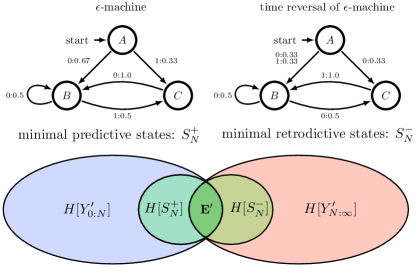
Figure 5: Alternate minimal generators of the Golden Mean Process: predictive and retrodictive. (Left) The $\epsilon$-machine has the minimal set of causal states $S^{+}$ required to predictively generate the output process. As a result, the uncertainty $\operatorname{H}[S^{+}_{N}]$ is contained by the uncertainty $\operatorname{H}[Y^{\prime}_{0:N}]$ in the output past. (Right) The time reversal of the reverse-time $\epsilon$-machine has the minimal set of states required to retrodictively generate the output. Its states are a function of the output future. Thus, its uncertainty $\operatorname{H}[S^{-}_{N}]$ is contained by the output future’s uncertainty $\operatorname{H}[Y^{\prime}_{N:\infty}]$.

These two different hidden Markov generators both produce the Golden Mean Process, and they provide a template for constructing ratchets to generate that process. For a hidden Markov model described by symbol-labeled transition matrix $\{T^{(y)}\}$, with hidden states in $\mathcal{S}$ as described in Eq. (19), the analogous generative ratchet has the same states $\mathcal{X}=\mathcal{S}$ and is described by the joint Markov local interaction:

$$M^{\text{local}}_{(x,y)\rightarrow(x^{\prime},y^{\prime})}=T^{(y^{\prime})}_{x\rightarrow x^{\prime}}~{}.$$

Such a ratchet effectively ignores the IID input process and obeys the same informational relationships between the ratchet states and outputs as the hidden states of hidden Markov model with its outputs.

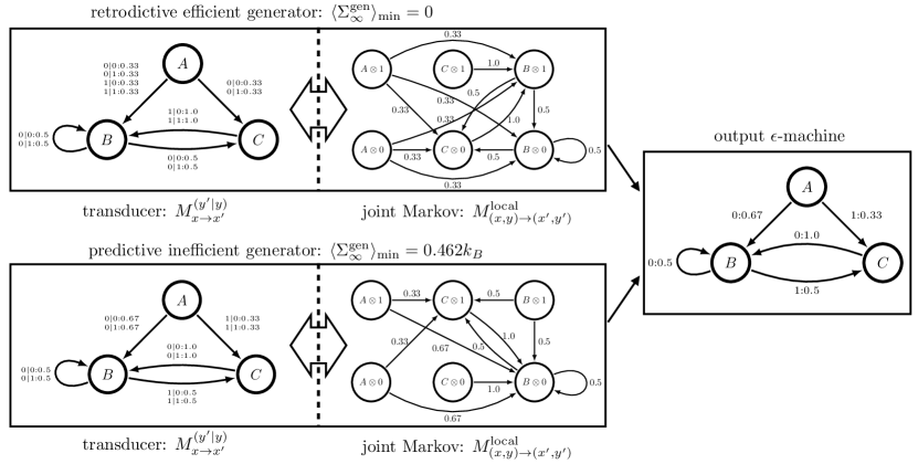
Figure 6: Alternative generators of the Golden Mean Process: (Right) The process’ $\epsilon$-machine. (Top row) Optimal generator designed using the topology of the minimal retrodictive generator. It is efficient, since it stores as little information about the past as possible, while still storing enough to generate the output. (Bottom row) The predictive generator stores far more information about the past than necessary, since it is based off the predictive $\epsilon$-machine. As a result, it is far less efficient. It dissipates at least $\tfrac{2}{3}k_{\text{B}}T\ln 2$ extra heat per symbol and requires that much more work energy per symbol emitted.

Figure 6 shows both the transducer and joint Markov representation of the minimal predictive generator and minimal retrodictive generator. The retrodictive generator is potentially perfectly efficient, since the process’ minimal modularity dissipation vanishes: $\langle\Sigma^{\text{gen}}_{N}\rangle_{\text{min}}=0$ for all $N$. However, despite being a standard tool for generating an output, the predictive $\epsilon$-machine is necessarily irreversible and dissipative. The $\epsilon$-machine-based ratchet, as shown in Fig. 6(bottom row), approaches an asymptotic dynamic where the current state $X_{N}$ stores more than it needs to about the past output past $Y^{\prime}_{0:N}$ in order to generate the future $Y^{\prime}_{N:\infty}$. As a result, it irretrievably dissipates:

$$\langle\Sigma^{\text{gen}}_{\infty}\rangle_{\text{min}} =k_{\text{B}}\ln 2\lim_{N\rightarrow\infty}(\operatorname{I}[Y^{\prime}_{0:N};X_{N}]\!-\!\operatorname{I}[Y^{\prime}_{0:N};X_{N+1},Y^{\prime}_{N}])$$

$$=\tfrac{2}{3}k_{\text{B}}\ln 2$$

$$\approx 0.462~{}k_{\text{B}}~{}.$$

With every time step, this predictive ratchet stores information about its past, but it also erases information, dissipating $2/3$ of a bit worth of correlations without leveraging them. Those correlations could have been used to reverse the process if they had been turned into work. They are used by the retrodictive ratchet, though, which stores just enough information about its past to generate the future.

It was previously shown that storing unnecessary information about the past leads to additional transient dissipation when generating a pattern [27, 19]. This cost also arises from implementation. However, our measure of modularity dissipation shows that there are implementation costs that persist through time. The two locally-operating generators of the Golden Mean Process perform the same computation, but have different bounds on their dissipation per time step. Thus, the additional work investment required to generate the process grows linearly with time for the $\epsilon$-machine implementation, but is zero for the retrodictive implementation.

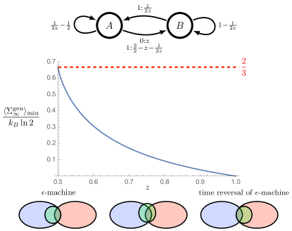
Figure 7: (Top) A parametrized family of HMMs that generate the Golden Mean Process for $z\in[.5,1]$. (Middle) As parameter $z$ increases, the information stored in the hidden states about the output past decreases. At $z=0.5$ the HMM is the $\epsilon$-machine, whose states are a function of the past. At $z=1.0$, the HMM is the time reversal of the reverse-time $\epsilon$-machine, whose states are a function of the future. The modularity dissipation decreases monotonically as $z$ increases and the hidden states’ memory of the past decreases. (Bottom) Information diagrams corresponding to the end cases and a middle case. Labeling as in Fig. 5.

Moreover, we can consider generators that fall in-between these extremes using the parametrized HMM shown in Fig. 7 (top). This HMM, parametrized by $z$, produces the Golden Mean Process at all $z\in[.5,1]$, but the hidden states share less and less information with the output past as $z$ increases, as shown by Ref. [31]. One extreme $z=0.5$ corresponds to the minimal predictive generator, the $\epsilon$-machine. The other at $z=1$ corresponds to the minimal retrodictive generator, the time reversal of the reverse-time $\epsilon$-machine. The graph there plots the modularity dissipation as a function of $z$. It decreases with $z$, suggesting that the unnecessary memory of the past leads to additional dissipation. So, while we have only proved that retrodictive generators are maximally efficient, this demonstrates that extending beyond that class can lead to unnecessary dissipation and that there may be a direct relationship between unnecessary memory and dissipation.

Taken altogether, we see that the thermodynamic consequences of localized information processing lead to direct principles for efficient information transduction. Analyzing the most general case of transducing arbitrary structured processes into other arbitrary structured processes remains a challenge. That said, pattern generators and pattern extractors have elegantly symmetric conditions for efficiency that give insight into the range of possibilities. Pattern generators are effectively the time-reversal of pattern extractors, which turn structured inputs into structureless outputs. As such they are most efficient when retrodictive, which is the time-reversal of being predictive. Figure 5 illustrated graphically how the predictive $\epsilon$-machine captures past correlations and stores the necessary information about the past, while the retrodictive ratchet’s states are analogous, but store information about the future instead. This may seem unphysical—as if the ratchet is anticipating the future. However, since the ratchet generates the output future, this anticipation is entirely physical, because the ratchet controls the future, as opposed to mysteriously predicting it, as an oracle would.

VI Conclusion

Modularity is a key design theme in physical information processing, since it gives the flexibility to stitch together many elementary logical operations to implement a much larger computation. Any classical computation can be composed from local operations on a subset of information reservoir observables. Modularity is also key to biological organization, its functioning, and our understanding of these [4].

However, there is an irretrievable thermodynamic cost, the modularity dissipation, to this localized computing, which we quantified in terms of the global entropy production. This modularity-induced entropy production is proportional to the reduction of global correlations between the local and interacting portion of the information reservoir and the fixed, noninteracting portion. This measure forms the basis for designing thermodynamically efficient information processing. It is proportional to the additional work investment required by the modular form of the computation, beyond the work required by a globally integrated and reversible computation.

Turing machine-like information ratchets provide a natural application for this new measure of efficient information processing, since they process information in a symbol string through a sequence of local operations. The modularity dissipation allows us to determine which implementations are able to achieve the asymptotic bound set by the IPSL which, substantially generalizing Landauer’s bound, says that any type of structure in the input can be used as a thermal resource and any structure in the output has a thermodynamic cost. There are many different ratchet implementations that perform a given computation, in that they map inputs to outputs in the same way. However, if we want an implementation to be thermodynamically efficient, the modularity dissipation, monitored by the global entropy production, must be minimized. Conversely, we now appreciate why there are many implementations that dissipate and are thus irreversible. This establishes modularity dissipation as a new thermodynamic cost, due purely to an implementation’s architecture, that complements Landauer’s bound on isolated logical operations.

We noted that there are not yet general principles for designing devices that minimize modularity dissipation and thus work investment for arbitrary information transduction. However, for the particular cases of pattern generation and pattern extraction we find that there are prescribed classes of ratchets that are guaranteed to be dissipationless, if operated quasistatically. The ratchet states of these devices are able to store and leverage the global correlations among the symbol strings, which means that it is possible to achieve the reversibility of globally integrated information processing but with modular computational design. Thus, while modular computation often results in dissipating global correlations, this inefficiency can be avoided when designing processors by employing the tools of computations mechanics outlined here.

Appendix A Quasistatic Markov Channels

To satisfy information-theoretic bounds on work dissipation, we describe a quasistatic channel where we slowly change system energies to manipulate the distribution over $\mathcal{Z}$’s states. Precisely, our challenge is to evolve over time interval $(t,t+\tau)$ an input distribution $\Pr(Z_{t}=z_{t})$ according the Markov channel $M$, so that system’s conditional probability at time $t+\tau$ is:

$$\Pr(Z_{t+\tau}=z_{t+\tau}|Z_{t}=z_{t})=M_{z_{t}\rightarrow z_{t+\tau}}~{}.$$

Making this as efficient as possible in a thermal environment at temperature $T$ means ensuring that the work invested in the evolution achieves the lower bound:

$$\langle W\rangle\geq k_{B}T\ln 2(\operatorname{H}[Z_{t}]-\operatorname{H}[Z_{t+\tau}])~{}.$$

This expresses the Second Law of Thermodynamics for the system in contact with a heat bath.

To ensure the appropriate conditional distribution, we introduce an ancillary system $\mathcal{Z}^{\prime}$, which is a copy of $\mathcal{Z}$. So that it is efficient, we take $\tau$ to be large with respect to the system’s relaxation time scale and break the overall process into three steps that occur over the time intervals $(t,t+\tau_{0})$, $(t+\tau_{0},t+\tau_{1})$, and $(t+\tau_{1},t+\tau)$, where $0<\tau_{0}<\tau_{1}<\tau$.

Our method of manipulating $\mathcal{Z}$ and $\mathcal{Z}^{\prime}$ is to control the energy $E(t,z,z^{\prime})$ of the joint state $z\otimes z^{\prime}\in\mathcal{Z}\otimes\mathcal{Z}^{\prime}$ at time $t$. We also control whether or not probability is allowed to flow in $\mathcal{Z}$ or $\mathcal{Z}^{\prime}$. This corresponds to raising or lowering energy barriers between system states.

At the beginning of the control protocol we choose $\mathcal{Z}^{\prime}$ to be in a uniform distribution uncorrelated with $\mathcal{Z}$. This means the joint distribution can be expressed:

$$\Pr(Z_{t}=z_{t},Z^{\prime}_{t}=z_{t}^{\prime})=\frac{\Pr(Z_{t}=z_{t})}{|\mathcal{Z}^{\prime}|}~{}.$$ (22)

Since we are manipulating an energetically mute information reservoir, we also start with the system in a uniformly zero-energy state over the joint states of $\mathcal{Z}$ and $\mathcal{Z}^{\prime}$:

$$E(t,z,z^{\prime})=0~{}.$$ (23)

While this energy and the distribution change when executing the protocol, we return $\mathcal{Z}^{\prime}$ to the independent uniform distribution and the energy to zero at the end of the protocol. This ensures consistency and modularity. However, the same results can be achieved by choosing other starting energies with $\mathcal{Z}^{\prime}$ in other distributions.

The three steps that evolve this system to quasistatically implement the Markov channel $M$ are as follows:

1. Over the time interval $(t,t+\tau_{0})$, continuously change the energy such that the energy at the end of the interval $E(t+\tau_{0},z,z^{\prime})$ obeys the relation:

   $$e^{-(E(t+\tau_{0},z,z^{\prime})-F(t+\tau_{0}))/k_{B}T}=\Pr(Z_{t}=z)M_{z\rightarrow z^{\prime}}~{},$$

   while allowing state space and probability to flow in $\mathcal{Z}^{\prime}$, but not in $\mathcal{Z}$. Since the protocol is quasistatic, $\mathcal{Z}^{\prime}$ follows the Boltzmann distribution and at time $t+\tau_{0}$ the distribution over $\mathcal{Z}\otimes\mathcal{Z}^{\prime}$ is:

   $$\Pr(Z_{t+\tau_{0}}=z,Z^{\prime}_{t+\tau_{0}}=z^{\prime})=\Pr(Z_{t}=z)M_{z\rightarrow z^{\prime}}~{}.$$

   This yields the conditional distribution of the current ancillary variable $Z^{\prime}_{t+\tau}$ on the initial system variable $Z_{t}$:

   $$\Pr(Z^{\prime}_{t+\tau_{0}}=z^{\prime}|Z_{t}=z)=M_{z\rightarrow z^{\prime}}~{},$$

   since the system variable $Z_{t}$ remains fixed over the interval. This protocol effectively applies the Markov channel $M$ to evolve from $\mathcal{Z}$ to $\mathcal{Z}^{\prime}$. However, we want the Markov channel to apply strictly to $\mathcal{Z}$.

   Being a quasistatic protocol, there is no entropy production and the work flow is simply the change in nonequilibrium free energy:

   $$\langle W_{1}\rangle =\Delta F^{\text{neq}}$$

   $$=\Delta\langle E\rangle-T\Delta S[Z,Z^{\prime}]~{}.$$

   Since the average initial energy is uniformly zero, the change in average energy is the average energy at time $t+\tau_{0}$. And so, we can express the work done:

   $$\langle W_{1}\rangle =\langle E(t+\tau_{0})\rangle-T\Delta S[Z,Z^{\prime}]$$

   $$=\langle E(t+\tau_{0})\rangle$$

   $$\qquad+k_{\text{B}}T\ln 2(\operatorname{H}[Z_{t},Z^{\prime}_{t}]-\operatorname{H}[Z_{t+\tau_{0}},Z_{t+\tau_{0}}^{\prime}])~{}.$$

2. Now, swap the states of $\mathcal{Z}$ and $\mathcal{Z}^{\prime}$ over the time interval $(t+\tau_{0},t+\tau_{1})$. This is logically reversible. Thus, it can be done without any work investment over the second time interval:

   $$\langle W_{2}\rangle=0~{}.$$ (24)

   The result is that the energies and probability distributions are flipped with regard to exchange of the system $\mathcal{Z}$ and ancillary system $\mathcal{Z}^{\prime}$:

   $$E(t+\tau_{1},z,z^{\prime}) =E(t+\tau_{0},z^{\prime},z)$$

   $$\Pr(Z_{t+\tau_{1}}\!=\!z,Z^{\prime}_{t+\tau_{1}}\!=\!z^{\prime}) =\Pr(Z_{t+\tau_{0}}\!=\!z^{\prime},Z^{\prime}_{t+\tau_{0}}\!=\!z)~{}.$$

   Most importantly, however, this means that the conditional probability of the current system variable is given by $M$:

   $$Pr(Z_{t+\tau_{1}}=z^{\prime}|Z_{t}=z) =\Pr(Z^{\prime}_{t+\tau_{0}}=z^{\prime}|Z_{t}=z)$$

   $$=M_{z\rightarrow z^{\prime}}~{}.$$

   The ancillary system must still be reset to a uniform and uncorrelated state and the energies must be reset.

3. Finally, we again hold $\mathcal{Z}$’s state fixed while allowing $\mathcal{Z}^{\prime}$ to change over the time interval $(t+\tau_{1},t+\tau)$ as we change the energy, ending at $E(t+\tau,z,z^{\prime})=0$. This quasistatically brings the joint distribution to one where the ancillary system is uniform and independent of $\mathcal{Z}$:

   $$\Pr(Z_{t+\tau}=z,Z_{t+\tau}^{\prime}=z^{\prime})=\frac{\Pr(Z_{t+\tau}=z)}{|\mathcal{Z}^{\prime}|}~{}.$$ (25)

   Again, the invested work is the change in average energy plus the change in thermodynamic entropy of the joint system:

   $$\langle W_{3}\rangle =\langle\Delta E\rangle$$

   $$\quad+k_{\text{B}}T\ln 2(\operatorname{H}[Z_{t+\tau_{1}},Z^{\prime}_{t+\tau_{1}}]-\operatorname{H}[Z_{t+\tau},Z_{t+\tau}^{\prime}])$$

   $$=-\langle E(t+\tau_{1})\rangle$$

   $$\quad+k_{\text{B}}T\ln 2(\operatorname{H}[Z_{t+\tau_{1}},Z^{\prime}_{t+\tau_{1}}]-\operatorname{H}[Z_{t+\tau},Z_{t+\tau}^{\prime}])~{}.$$

   This ends this three-step protocol.

Summing up the heat terms, gives the total dissipation:

$$\langle W_{\text{total}}\rangle =\langle W_{t}\rangle+\langle W_{2}\rangle+\langle W_{3}\rangle$$

$$=k_{\text{B}}T\ln 2(\operatorname{H}[Z_{t},Z^{\prime}_{t}]-\operatorname{H}[Z_{t+\tau_{0}},Z_{t+\tau_{0}}^{\prime}])$$

$$\quad+k_{\text{B}}T(\operatorname{H}[Z_{t+\tau_{1}},Z^{\prime}_{t+\tau_{1}}]-\operatorname{H}[Z_{t+\tau},Z_{t+\tau}^{\prime}])$$

$$\quad+\langle E(t+\tau_{0})\rangle-\langle E(t+\tau_{1})\rangle~{}.$$

Recall that the distributions $\Pr(Z_{t+\tau_{1}},Z^{\prime}_{t+\tau_{1}})$ and $\Pr(Z_{t+\tau_{0}},Z_{t+\tau_{0}}^{\prime})$, as well as $E(t+\tau_{0},z,z^{\prime})$ and $E(t+\tau_{1},z,z^{\prime})$, are identical under exchange of $\mathcal{Z}$ and $\mathcal{Z}^{\prime}$, so $H[Z_{t+\tau_{1}},Z^{\prime}_{t+\tau_{1}}]=H[Z_{t+\tau_{0}},Z_{t+\tau_{0}}^{\prime}]$ and $\langle E(t+\tau_{0})\rangle=\langle E(t+\tau_{1})\rangle$. Additionally, we know that both the starting and ending distributions have a uniform and uncorrelated ancillary system, so their entropies can be expressed:

$$\operatorname{H}[Z_{t},Z^{\prime}_{t}] =\operatorname{H}[Z_{t}]+\log_{2}|\mathcal{Z}^{\prime}|$$ (26)

$$\operatorname{H}[Z_{t+\tau},Z^{\prime}_{t+\tau}] =\operatorname{H}[Z_{t+\tau}]+\log_{2}|\mathcal{Z}^{\prime}|~{}.$$ (27)

Substituting this in to the above expression for total invested work, we find that we achieve the lower bound with this protocol:

$$\langle W_{\text{total}}\rangle=k_{\text{B}}T\ln 2(\operatorname{H}[Z_{t}]-\operatorname{H}[Z_{t+\tau}])~{}.$$ (28)

Thus, the protocol implements a Markov channel that achieves the information-theoretic bounds. It is similar to that described in Ref. [19].

The basic principle underlying the protocol is that when manipulating system energies to change state space, choose the energies so that there is no instantaneous probability flow. That is, if one stops changing the energies, the distribution will not change. However, there are cases in which it is impossible prevent instantaneous flow. Then, there are necessarily inefficiencies that arise from the dissipation of the distribution flowing out of equilibrium.

Appendix B Transducer Dissipation

B.1 Predictive Extractors

For a pattern extractor, being reversible means that the transducer is predictive of the input process. More precisely, an extracting transducer that produces zero entropy is equivalent to it being a predictor of its input.

As discussed earlier, a reversible extractor satisfies:

$$\operatorname{I}[Y_{N+1:\infty};X_{N+1}]=\operatorname{I}[Y_{N+1:\infty};X_{N}Y_{N}]~{},$$

for all $N$, since it must be reversible at every step to be fully reversible. The physical ratchet being predictive of the input means two things. It means that $X_{N}$ shields the past $Y_{0:N}$ from the future $Y_{N:\infty}$. This is equivalent to the mutual information between the past and future vanishing when conditioned on the ratchet state:

$$\operatorname{I}[Y_{0:N};Y_{N:\infty}|X_{N}]=0~{}.$$

Note that this also implies that any subset of the past or future is independent of any other subset conditioned on the ratchet state:

$$\operatorname{I}[Y_{a:b};Y_{c:d}|X_{N}]=0\text{ where }b\leq N\text{ and }c\geq N~{}.$$

The other feature of a predictive transducer is that the past shields the ratchet state from the future:

$$\operatorname{I}[X_{N};Y_{N:\infty}|Y_{0:N}]=0~{}.$$

This is guaranteed by the fact that transducers are nonanticipatory: they cannot predict future inputs outside of their correlations with past inputs.

We start by showing that if the ratchet is predictive, then the entropy production vanishes. It is useful to note that being predictive is equivalent to being as anticipatory as possible and having:

$$\operatorname{I}[X_{N};Y_{N:\infty}]=\operatorname{I}[Y_{0:N};Y_{N:\infty}]~{},$$

which can be seen by subtracting $\operatorname{I}[Y_{0:N};Y_{N:\infty};X_{N}]$ from each side of the immediately preceding expression. Thus, it is sufficient to show that the mutual information between the partial input future $Y_{N+1:\infty}$ and the joint distribution of the predictive variable $X_{N}$ and next output $Y_{N}$ is the same as mutual information with the joint variable $(Y_{0:N},Y_{N})=Y_{0:N+1}$ of the past inputs and the next input:

$$\operatorname{I}[Y_{N+1:\infty};X_{N},Y_{N}]=\operatorname{I}[Y_{N+1:\infty};Y_{0:N},Y_{N}]~{}.$$

To show this for a predictive variable, we use Fig. 8, which displays the information diagram for all four variables with the information atoms of interest labeled.

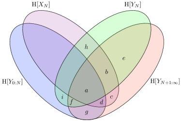
Figure 8: Information diagram for dependencies between the input past $Y_{0:N}$, next input $Y_{N}$, current ratchet state $X_{N}$, and input future $Y_{N+1:\infty}$, excluding the next input. We label certain information atoms to help illustrate the algebraic steps in the associated proof.

Assuming that $X_{N}$ is predictive zeros out a number of information atoms, as shown below:

$$\operatorname{I}[X_{N};Y_{N},Y_{N+1:\infty}|Y_{0:N}] =b+c+h=0$$

$$\operatorname{I}[X_{N};Y_{N}|Y_{0:N}] =b+h=0$$

$$\operatorname{I}[Y_{0:N};Y_{N},Y_{N+1:\infty}|X_{N}] =i+f+g=0$$

$$\operatorname{I}[Y_{0:N};Y_{N}|X_{N}] =i+f=0~{}.$$

These four equations make it clear that $g=c=0$. Thus, substituting $\operatorname{I}[Y_{N+1:\infty};X_{N},Y_{N}]=a+b+c+d+e+f$ and $\operatorname{I}[Y_{N+1:\infty};Y_{0:N},Y_{N}]=a+b+d+e+f+g$, we find that their difference vanishes:

$$\operatorname{I}[Y_{N+1:\infty};X_{N},Y_{N}]-I[Y_{N+1:\infty};Y_{0:N},Y_{N}] =c-g$$

$$=0~{}.$$

There is zero dissipation, since $X_{N+1}$ is also predictive, meaning $\operatorname{I}[Y_{N+1:\infty};Y_{0:N},Y_{N}]=\operatorname{I}[Y_{N+1:\infty};X_{N+1}]$, so:

$$\frac{\langle\Sigma^{\text{ext}}_{N}\rangle_{\text{min}}}{k_{\text{B}}T\ln 2} =\operatorname{I}[Y_{N+1:\infty};X_{N},Y_{N}]-I[Y_{N+1:\infty};X_{N+1}]$$

$$=\operatorname{I}[Y_{N+1:\infty};X_{N},Y_{N}]-I[Y_{N+1:\infty};Y_{0:N+1}]$$

$$=0~{}.$$

Going the other direction, using zero entropy production to prove that $X_{N}$ is predictive for all $N$ is now simple.

We already showed that $\operatorname{I}[Y_{N+1:\infty};X_{N},Y_{N}]=\operatorname{I}[Y_{N+1:\infty};Y_{0:N},Y_{N}]$ if $X_{N}$ is predictive. Combining with zero entropy production ($\operatorname{I}[Y_{N+1:\infty};X_{N+1}]=\operatorname{I}[Y_{N+1:\infty};X_{N},Y_{N}]$) immediately implies that $X_{N+1}$ is predictive, since $\operatorname{I}[Y_{N+1:\infty};X_{N+1}]=\operatorname{I}[Y_{N+1:\infty};Y_{0:N},Y_{N}]$ plus the fact that $X_{N+1}$ is equivalent to $X_{N+1}$ being predictive.

With this recursive relation, all that is left to establish is the base case, that $X_{0}$ is predictive. Applying zero entropy production again we find the relation necessary for prediction:

$$\operatorname{I}[Y_{1:\infty};X_{1}] =\operatorname{I}[Y_{1:\infty};X_{0},Y_{0}]$$

$$=\operatorname{I}[Y_{1:\infty};Y_{0}]~{},$$

From this, we find the equivalence $\operatorname{I}[Y_{1:\infty};Y_{0}]=\operatorname{I}[Y_{1:\infty};X_{0},Y_{0}]$, since $X_{0}$ is independent of all inputs, due to it being nonanticipatory. Thus, zero entropy production is equivalent to predictive ratchets for pattern extractors.

B.2 Retrodictive Generators

An analogous argument can be made to show the relationship between retrodiction and zero entropy production for pattern generators, which are essentially time reversed extractors.

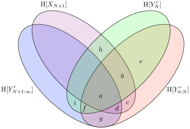
Figure 9: Information shared between the output past $Y^{\prime}_{0:N}$, next output $Y^{\prime}_{N}$, next ratchet state $X_{N+1}$, and output future $Y^{\prime}_{N+1:\infty}$, excluding the next input. Key information atoms are labeled.

Efficient pattern generators must satisfy:

$$\operatorname{I}[Y_{0:N}^{\prime};X_{N}]=\operatorname{I}[Y_{0:N}^{\prime};X_{N+1}Y_{N}^{\prime}]~{}.$$

The ratchet being retrodictive means that the ratchet state $X_{N}$ shields the past $Y^{\prime}_{0:N}$ from the future $Y^{\prime}_{N:\infty}$ and that the future shields the ratchet from the past:

$$\operatorname{I}[Y^{\prime}_{0:N};Y^{\prime}_{N:\infty}|X_{N}] =0$$

$$\operatorname{I}[Y^{\prime}_{0:N};X_{N}|Y^{\prime}_{N:\infty}] =0~{}.$$

Note that generators necessarily shield past from future $\operatorname{I}[Y^{\prime}_{0:N};Y^{\prime}_{N:\infty}|X_{N}]=0$, since all temporal correlations must be stored in the generator’s states. Thus, for a generator, being retrodictive is equivalent to:

$$\operatorname{I}[Y^{\prime}_{0:N};X_{N}]=\operatorname{I}[Y^{\prime}_{0:N};Y^{\prime}_{N:\infty}]~{}.$$

This can be seen by subtracting $\operatorname{I}[Y^{\prime}_{0:N};X_{N};Y^{\prime}_{N:\infty}]$ from both sides, much as done with the extractor.

First, to show that being retrodictive implies zero minimal entropy production, it is sufficient to show that:

$$\operatorname{I}[Y_{0:N}^{\prime};X_{N+1},Y_{N}^{\prime}]=\operatorname{I}[Y_{0:N}^{\prime};Y_{N:\infty}^{\prime}]~{},$$

since we know that $\operatorname{I}[Y_{0:N}^{\prime};X_{N}]=\operatorname{I}[Y_{0:N}^{\prime};Y_{N:\infty}^{\prime}]$. To do this, consider the information diagram in Fig. 9. There we see that the difference between the two mutual informations of interest reduce to the difference between the two information atoms:

$$\operatorname{I}[Y_{0:N}^{\prime};X_{N+1}Y_{N}^{\prime}]-\operatorname{I}[Y_{0:N}^{\prime};Y_{N:\infty}^{\prime}]=c-g~{}.$$

The fact that the ratchet state $X_{N+1}$ shields the past $Y^{\prime}_{0:N+1}$ from the future $Y^{\prime}_{N+1:\infty}$ and the future shields the ratchet from the past gives us the following four relations:

$$\operatorname{I}[Y^{\prime}_{0:N}Y^{\prime}_{N};Y^{\prime}_{N+1:\infty}|X_{N+1}] =i+f+g=0$$

$$\operatorname{I}[Y^{\prime}_{N};Y^{\prime}_{N+1:\infty}|X_{N+1}] =i+f=0$$

$$\operatorname{I}[Y^{\prime}_{0:N}Y^{\prime}_{N};X_{N+1}|Y^{\prime}_{N+1:\infty}] =h+b+c=0$$

$$\operatorname{I}[Y^{\prime}_{N};X_{N+1}|Y^{\prime}_{N+1:\infty}] =h+b=0~{}.$$

These equations show that that $c=g=0$ and thus:

$$\frac{\langle\Sigma^{\text{gen}}_{N}\rangle_{\text{min}}}{k_{\text{B}}T\ln 2}=0~{}.$$

Going the other direction—zero entropy production implies retrodiction—requires that we use $\operatorname{I}[Y_{0:N}^{\prime};X_{N}]=\operatorname{I}[Y_{0:N}^{\prime};X_{N+1},Y_{N}^{\prime}]$ to show $\operatorname{I}[Y^{\prime}_{0:N};X_{N}]=\operatorname{I}[Y^{\prime}_{0:N};Y^{\prime}_{N:\infty}]$. If $X_{N+1}$ is retrodictive, then we can show that $X_{N}$ must be as well. However, this makes the base case of the recursion difficult, since there is not yet a reason to conclude that $X_{\infty}$ is retrodictive. While we conjecture the equivalence of optimally retrodictive generators and efficient generators, at this point we can only conclusively say that retrodictive generators are also efficient.

References

- [1] R. Landauer. Irreversibility and heat generation in the computing process. IBM J. Res. Develop., 5(3):183–191, 1961.
- [2] E. Fredkin and T. Toffoli. Conservative logic. Intl. J. Theo. Phys., 21(3/4):219–253, 1982.
- [3] F. Rieke, D. Warland, R. de Ruyter van Steveninck, and W. Bialek. Spikes: Exploring the Neural Code. Bradford Book, New York, 1999.
- [4] U. Alon. An Introduction to Systems Biology: Design Principles of Biological Circuits. Chapman and Hall/CRC, Boca Raton, Lousiana, 2007.
- [5] K. Ulrich. Fundamentals of modularity. In S. Dasu and C. Eastman, editors, Management of Design, pages 219–231. Springr, Amsterdam, Netherlands, 1994.
- [6] C.-C. Chen and N. Crilly. From modularity to emergence: a primer on design and science of complex systems. Technical Report CUED/C-EDC/TR.155, Department of Engineering, University of Cambridge, Cambridge, United Kingdom, September 2016.
- [7] J. Maynard-Smith and E. Szathmary. The Major Transitions in Evolution. Oxford University Press, Oxford, reprint edition, 1998.
- [8] A. B. Boyd, D. Mandal, and J. P. Crutchfield. Correlation-powered information engines and the thermodynamics of self-correction. Phys. Rev. E, 95(1):012152, 2017.
- [9] S. Lloyd. Use of mutual information to decrease entropy: Implications for the second law of thermodynamics. Phys. Rev. A, 39:5378–5386, 1989.
- [10] R. Storn and K. Price. Differential evolution - a simple and efficient heuristic for global optimization over continuous space. J. Global Optim., 11(341-359), 1997.
- [11] J. D. Lohn, G. S. Hornby, and D. S. Linden. An evolved antenna for deployment on nasa’s space technology 5 mission. In U.-M. O’Reilly, T. Yu, R. Riolo, and B. Worzel, editors, Genetic Programming Theory and Practice II, pages 301–315. Springer US, New York, 2005.
- [12] J. Koza. Genetic Programming: On the Programming of Computers by Means of Natural Selection. Bradford Book, New York, 1992.
- [13] D. Mandal and C. Jarzynski. Work and information processing in a solvable model of Maxwell’s demon. Proc. Natl. Acad. Sci. USA, 109(29):11641–11645, 2012.
- [14] A. B. Boyd, D. Mandal, and J. P. Crutchfield. Identifying functional thermodynamics in autonomous Maxwellian ratchets. New J. Physics, 18:023049, 2016.
- [15] N. Merhav. Sequence complexity and work extraction. J. Stat. Mech., page P06037, 2015.
- [16] A. B. Boyd, D. Mandal, and J. P. Crutchfield. Leveraging environmental correlations: The thermodynamics of requisite variety. J. Stat. Phys., 167(6):1555–1585, 2016.
- [17] N. Barnett and J. P. Crutchfield. Computational mechanics of input-output processes: Structured transformations and the -transducer. J. Stat. Phys., 161(2):404–451, 2015.
- [18] J. G. Brookshear. Theory of computation: Formal languages, automata, and complexity. Benjamin/Cummings, Redwood City, California, 1989.
- [19] A. J. P. Garner, J. Thompson, V. Vedral, and M. Gu. When is simpler thermodynamically better? arXiv, 1510.00010, 2015.
- [20] J. M. R. Parrondo, J. M. Horowitz, and T. Sagawa. Thermodynamics of information. Nature Physics, 11(2):131–139, February 2015.
- [21] S. Still. Thermodynamic cost and benefit of data representations. arXiv:1705.00612v1, 2017.
- [22] Z. Lu, D. Mandal, and C. Jarzynski. Engineering Maxwell’s demon. Physics Today, 67(8):60–61, January 2014.
- [23] A. Turing. On computable numbers, with an application to the Entschiedungsproblem. Proc. Lond. Math. Soc., 42, 43:230–265, 544–546, 1937.
- [24] Space limitations here do not allow a full digression on possible implementations. Suffice it to say that for unidirectional tape reading, the ratchet state requires a storage register or an auxiliary internal working tape as portrayed in Fig. 3 of Ref. [32].
- [25] C. E. Shannon. A universal Turing machine with two internal states. In C. E. Shannon and J. McCarthy, editors, Automata Studies, number 34 in Annals of Mathematical Studies, pages 157–165. Princeton University Press, Princeton, New Jersey, 1956.
- [26] M. Minsky. Computation: Finite and Infinite Machines. Prentice-Hall, Englewood Cliffs, New Jersey, 1967.
- [27] A. B. Boyd, D. Mandal, P. M. Riechers, and J. P. Crutchfield. Transient dissipation and structural costs of physical information transduction. Phys. Rev. Lett., 118:220602, 2017.
- [28] P. Strasberg, J. Cerrillo, G. Schaller, and T. Brandes. Thermodynamics of stochastic Turing machines. Phys. Rev. E, 92(4):042104, 2015.
- [29] N. Merhav. Relations between work and entropy production for general information-driven, finite-state engines. J. Stat. Mech.: Th. Expt., 2017:1–20, 2017.
- [30] J. P. Crutchfield and D. P. Feldman. Regularities unseen, randomness observed: Levels of entropy convergence. CHAOS, 13(1):25–54, 2003.
- [31] C. J. Ellison, J. R. Mahoney, R. G. James, J. P. Crutchfield, and J. Reichardt. Information symmetries in irreversible processes. CHAOS, 21(3):037107, 2011.
- [32] J. P. Crutchfield. The calculi of emergence: Computation, dynamics, and induction. Physica D, 75:11–54, 1994.