Data recovery: from limited-aperture to full-aperture

Abstract

The inverse scattering problems have been popular for the past thirty years. While very successful in many cases, progress has lagged when only limited-aperture measurement is available. In this paper, we perform some elementary study to recover data that can not be measured directly. To be precise, we aim at recovering the full-aperture far field data from limited-aperture measurement. Due to the reciprocity relation, the multi-static response matrix (MSR) has a symmetric structure. Using the Green’s formula and single layer potential, we propose two schemes to recover full-aperture MSR. The recovered data is tested by a recently proposed direct sampling method and the factorization method. The numerical results show the possibility to recover, at least partially, the missing data and consequently improve the reconstruction of the scatterer.

Keywords: inverse scattering, multi-static response matrix, limited-aperture, data recovery.

AMS subject classifications: 35P25, 35Q30, 45Q05, 78A46

1 Introduction

The inverse scattering theory has been a fast-developing area for the past thirty years. The aim is to detect and identify the unknown objects using acoustic, electromagnetic, or elastic waves. Many methods have been proposed, e.g., iterative methods, decomposition methods, the linear sampling method, the factorization method and direct sampling methods [4, 5, 6, 7, 9, 11, 13, 14, 15, 18, 19, 23, 24]. Most of the above algorithms use full-aperture data, i.e., data of all the observation directions due to all incident directions. However, in many cases of practical interest, it is not possible to measure the full-aperture data, e.g., underground mineral prospection, mine location in the battlefield, and anti-submarine detection. Consequently, only limited-aperture data over a range of angles are available.

Various reconstruction algorithms using limited-aperture data have been developed [1, 3, 10, 12, 14, 17, 20, 21, 25]. Although uniqueness of the inverse problems can be proved in some cases [8], the quality of the reconstructions are not satisfactory. Indeed, limited-aperture data put forward a severe challenge for all the existing numerical methods. A typical feature is that the "shadow region" is elongated in down range [17]. Physically, the information from the "shadow region" is very weak, especially for high frequency waves [20]. For two-dimensional problems, the numerical experiments of the decomposition methods in [12, 25] indicate that satisfactory reconstructions need an aperture not smaller than 180 degrees.

Other than developing methods using limited-aperture data, we take an alternative approach to recover the data that can not be measured directly. As a consequence, methods using full-aperture data can be employed. We take the acoustic scattering by time-harmonic plane waves as the model problem. The measurement data are only available for limited-aperture observation angles but for all incident directions. The goal is to recover data for all observation angles. The case to recover full-aperture data from limited-aperture observation angles due to limited-aperture incident directions will be considered in future.

For scattering problems, it is well-known that the full-aperture data can be uniquely determined by the limited-aperture data. However, because of the severely ill-posed nature of the analytic continuation, it is in general not possible to recover full-aperture data using techniques such as extrapolation [2]. We take a different way by seeking an analytic function in a suitable space based on the PDE theory governing the scattering problem. More precisely, we look for kernels of layer potentials that generate the measured data approximately by regularization. Then these kernels are used to obtain the full-aperture data.

This paper is organized as follows. In Section 2, we briefly introduce the scattering problem of interests and the multi-static response (MSR) matrix, which is the far field pattern. Due to the reciprocity relation of the far field pattern, the MSR has a symmetry property, which can be used to recover partial missing data. In Section 3.1, we propose a technique using the Green’s formula to recover the full MSR. Another recovery technique based on the single layer potential is proposed in subsection 3.2. Combining these techniques and the symmetry property, a novel algorithm is proposed to recover the full-aperture MSR. In Section 4, numerical examples are presented to demonstrate the performance of the data recover techniques. The recovered data are tested using a direct sampling method and the factorization method. We draw some conclusions and discuss future works in Section 5.

2 The Multi-static Response Matrix

Let $k$ be the wave number of a time harmonic wave and $\Omega\subset{\mathbb{R}}^{n}(n=2,\,3)$ be a bounded domain with Lipschitz-boundary $\partial\Omega$ such that the exterior ${\mathbb{R}}^{n}\backslash\overline{\Omega}$ is connected. Let the incident field $u^{i}$ be given by

$$u^{i}(x)\ =\ u^{i}(x;d)=e^{ikx\cdot d},\quad x\in{\mathbb{R}}^{n}\,,$$ (2.1)

where $d\in S^{n-1},S^{n-1}:=\{x\in{\mathbb{R}}^{n}:|x|=1\}$, denotes the direction of the plane wave.

The scattering problem for an inhomogeneous medium is to find the total field $u=u^{i}+u^{s}$ such that

$$\Delta u+k^{2}(1+q)u=0\quad\mbox{in }{\mathbb{R}}^{n},$$ (2.2)

$$\lim_{r:=|x|\rightarrow\infty}r^{\frac{n-1}{2}}\left(\frac{\partial u^{s}}{\partial r}-iku^{s}\right)=\,0,$$ (2.3)

where $q\in L^{\infty}({\mathbb{R}}^{n})$ such that its imaginary part $\Im(q)\geq 0$ and $q=0$ in ${\mathbb{R}}^{n}\backslash\overline{\Omega}$. The Sommerfeld radiation condition (2.3) holds uniformly with respect to all directions $\hat{x}:=x/|x|\in S^{n-1}$. If the scatterer $\Omega$ is impenetrable, the direct scattering problem is to find the total field $u=u^{i}+u^{s}$ such that

$$\Delta u+k^{2}u=0\quad\mbox{in }{\mathbb{R}}^{n}\backslash\overline{\Omega},$$ (2.4)

$$\mathcal{B}(u)=0\quad\mbox{on }\partial\Omega,$$ (2.5)

$$\lim_{r:=|x|\rightarrow\infty}r^{\frac{n-1}{2}}\left(\frac{\partial u^{s}}{\partial r}-iku^{s}\right)=\,0,$$ (2.6)

where $\mathcal{B}$ denotes one of the following three boundary conditions:

$$(1)\,\mathcal{B}(u):=u\,\,\mbox{on}\ \partial\Omega;\qquad(2)\,\mathcal{B}(u):=\frac{\partial u}{\partial\nu}\,\,\mbox{on}\ \partial\Omega;\qquad(3)\,\mathcal{B}(u):=\frac{\partial u}{\partial\nu}+\lambda u\,\,\mbox{on}\ \partial\Omega$$

corresponding, respectively, to the cases when the scatterer $\Omega$ is sound-soft, sound-hard, and of the impedance type. Here, $\nu$ is the unit outward normal to $\partial\Omega$ and $\lambda\in L^{\infty}(\partial\Omega)$ is the (complex valued) impedance function such that $\Im(\lambda)\geq 0$ almost everywhere on $\partial\Omega$. Uniqueness of the scattering problems (2.2)–(2.3) and (2.4)–(2.6) can be shown with the help of Green’s theorem, Rellich’s lemma and unique continuation principle, see e.g., [8]. The proof of existence can be done by variational approaches (cf. [8, 22] for the Dirichlet boundary condition and [4] for other boundary conditions) or by integral equation methods (cf. [8]).

Radiating solutions of the Helmholtz equation have the following asymptotic behavior [14, 18]:

$$u^{s}(x;d)=\frac{e^{i\frac{\pi}{4}}}{\sqrt{8k\pi}}\left(e^{-i\frac{\pi}{4}}\sqrt{\frac{k}{2\pi}}\right)^{n-2}\frac{e^{ikr}}{r^{\frac{n-1}{2}}}\left\{u^{\infty}(\hat{x};d)+\mathcal{O}\left(\frac{1}{r}\right)\right\}\quad\mbox{as }\,r:=|x|\rightarrow\infty$$ (2.7)

uniformly with respect to all directions $\hat{x}:=x/|x|\in S^{n-1}$. The complex valued function $u^{\infty}(\hat{x})=u^{\infty}(\hat{x};d)$ defined on the unit sphere $S^{n-1}$ is known as the scattering amplitude or far-field pattern with $\hat{x}\in S^{n-1}$ denoting the observation direction.

It is well known that the scatterer $\Omega$ can be uniquely determined by the far field pattern $u^{\infty}(\hat{x},d)$ for all $\hat{x},d\in S^{n-1}$ [8]. Due to analyticity, $u^{\infty}(\hat{x},d)$ for $(\hat{x},d)\in S^{n-1}\times S^{n-1}$ is uniquely determined by $u^{\infty}(\hat{x},d)$ for $(\hat{x},d)\in S_{0}^{n-1}\times S^{n-1}$ if $S_{0}^{n-1}\subsetneq S^{n-1}$ has a nonempty interior. Unfortunately, it is practically impossible to obtain $u^{\infty}(\hat{x},d)$ on $S^{n-1}$ from $u^{\infty}(\hat{x},d)$ on $S_{0}^{n-1}$ using the analytic continuation (see Atkinson [2]).

In this paper, we consider the discrete version of $u^{\infty}(\hat{x},d)$, i.e., the multi-static response (MSR) matrix in ${\mathbb{R}}^{2}$. Let $\theta_{i}:=(i-1)\pi/m,\,i=1,2,\ldots,2m$,

$$d_{i}:=(\cos\theta_{i},\sin\theta_{i}),\quad i=1,2,\ldots,2m,$$

and

$$\hat{x}_{j}:=(\cos\theta_{j},\sin\theta_{j}),\quad j=1,2,\ldots,2m.$$

The multi-static response (MSR) matrix $\mathbb{F}_{full}\in{\mathbb{C}}^{2m\times 2m}$ is defined as

$$\mathbb{F}_{full}:=\left(\begin{array}[]{cccc}u_{1,1}^{\infty}\quad u_{1,2}^{\infty}\quad\cdots\quad u_{1,2m}^{\infty}\\ u_{2,1}^{\infty}\quad u_{2,2}^{\infty}\quad\cdots\quad u_{2,2m}^{\infty}\\ \vdots\,\qquad\vdots\,\quad\ddots\,\qquad\vdots\\ u_{2m,1}^{\infty}\,\,u_{2m,2}^{\infty}\,\,\cdots\quad u_{2m,2m}^{\infty}\\ \end{array}\right),$$ (2.12)

where $u^{\infty}_{i,j}=u^{\infty}(\hat{x}_{j};d_{i})$ for $1\leq i,j\leq 2m$ corresponding to $2m$ observation directions $\hat{x}_{j}$ and $2m$ incident directions $d_{i}$.

Assume that the far field pattern can only be measured in a limited-aperture. In particular, the measured data are the first $l$ columns of $\mathbb{F}_{full}$

$$\mathbb{F}^{(l)}_{limit}:=\left(\begin{array}[]{cccc}u_{1,1}^{\infty}\,u_{1,2}^{\infty}\,\cdots\,u_{1,l}^{\infty}\\ u_{2,1}^{\infty}\,u_{2,2}^{\infty}\,\cdots\,u_{2,l}^{\infty}\\ \vdots\,\quad\vdots\,\quad\ddots\,\quad\vdots\\ u_{2m,1}^{\infty}\,u_{2m,2}^{\infty}\,\cdots\,u_{2m,l}^{\infty}\\ \end{array}\right),\quad 1\leq l<2m.$$ (2.17)

The inverse problem considered in this paper is to firstly recover $\mathbb{F}_{full}$ from $\mathbb{F}^{(l)}_{limit}$, and then reconstruct the scatterer $\Omega$ from the recovered $\mathbb{F}_{full}$. Note that $\mathbb{F}_{full}$ is NOT symmetric, i.e., $\mathbb{F}_{full}\neq\mathbb{F}_{full}^{T}$. Here and throughout the paper we use the superscript $"T"$ to denote the transpose of a matrix. We can partition the $2m$-by-$2m$ MSR matrix $\mathbb{F}_{full}$ into a $2$-by-$2$ block matrix

$$\mathbb{F}_{full}=\left(\begin{array}[]{cc}\mathbb{F}_{11}&\mathbb{F}_{12}\\ \mathbb{F}_{21}&\mathbb{F}_{22}\\ \end{array}\right),$$ (2.20)

where $\mathbb{F}_{ij}\in{\mathbb{C}}^{m\times m},i,j=1,2$. The following theorem is a consequence of the reciprocity relation.

Theorem 2.1.

$\mathbb{F}_{11}=\mathbb{F}_{22}^{T},\quad\mathbb{F}_{12}=\mathbb{F}_{12}^{T}$ and $\mathbb{F}_{21}=\mathbb{F}_{21}^{T}$.

Proof.

Recall that the far field pattern is the same if the direction of the incident field and the observation direction are interchanged [8], i.e.,

$$u^{\infty}(\hat{x},d)=u^{\infty}(-d,-\hat{x}),\quad\mbox{for all}\,\,\hat{x},d\in S^{1}.$$ (2.21)

For all $u^{\infty}_{i,j}\in\mathbb{F}_{11}$, using the reciprocity relation (2.21), we have

$$u^{\infty}_{i,j} = u^{\infty}(\hat{x}_{j};d_{i})$$

$$= u^{\infty}(-d_{i};-\hat{x}_{j})$$

$$= u^{\infty}(-(\cos\theta_{i},\sin\theta_{i});-(\cos\theta_{j},\sin\theta_{j}))$$

$$= u^{\infty}((\cos(\theta_{i}+\pi),\sin(\theta_{i}+\pi));(\cos(\theta_{j}+\pi),\sin(\theta_{j}+\pi)))$$

$$= u^{\infty}((\cos\theta_{i+m},\sin\theta_{i+m});(\cos\theta_{j+m},\sin\theta_{j+m}))$$

$$= u^{\infty}_{j+m,i+m},\quad 1\leq i,j\leq m.$$

Thus, we have $\mathbb{F}_{11}=\mathbb{F}_{22}^{T}$.

Similarly, For all $u^{\infty}_{i,j+m}\in\mathbb{F}_{12}$, using the reciprocity relation (2.21) again, we have

$$u^{\infty}_{i,j+m} = u^{\infty}(\hat{x}_{j+m};d_{i})$$

$$= u^{\infty}(-d_{i};-\hat{x}_{j+m})$$

$$= u^{\infty}(-(\cos\theta_{i},\sin\theta_{i});-(\cos\theta_{j+m},\sin\theta_{j+m}))$$

$$= u^{\infty}((\cos(\theta_{i}+\pi),\sin(\theta_{i}+\pi));(\cos(\theta_{j+m}+\pi),\sin(\theta_{j+m}+\pi)))$$

$$= u^{\infty}((\cos\theta_{i+m},\sin\theta_{i+m});(\cos\theta_{j},\sin\theta_{j}))$$

$$= u^{\infty}_{j,i+m},\quad 1\leq i,j\leq m.$$

Thus, we have $\mathbb{F}_{12}=\mathbb{F}_{12}^{T}$. The equality $\mathbb{F}_{21}=\mathbb{F}_{21}^{T}$ can be treated analogously. ∎

As a direct consequence of Theorem 2.1, the following data

$$\widetilde{\mathbb{F}}^{(l)}_{limit}:=\left(\begin{array}[]{cccc}u_{m+1,l+1}^{\infty}\,u_{m+1,l+2}^{\infty}\,\cdots\,u_{m+1,2m}^{\infty}\\ u_{m+2,l+1}^{\infty}\,u_{m+2,l+2}^{\infty}\,\cdots\,u_{m+2,2m}^{\infty}\\ \vdots\,\qquad\vdots\,\qquad\ddots\,\qquad\vdots\\ u_{m+l,l+1}^{\infty}\,u_{m+l,l+2}^{\infty}\,\cdots\,u_{m+l,2m}^{\infty}\\ \end{array}\right),\quad 1\leq l<2m,$$ (2.26)

can be obtained directly from $\mathbb{F}^{(l)}_{limit}$. Here, we have set $u_{i,j}^{\infty}:=u_{i-2m,j}^{\infty}$ if $i>2m,1\leq j<2m$.

Remark 2.2.

If we set

$$\widehat{\mathbb{F}}_{full}:=\left(\begin{array}[]{cc}\mathbb{F}_{12}&\mathbb{F}_{11}\\ \mathbb{F}_{22}&\mathbb{F}_{21}\\ \end{array}\right),$$

then $\widehat{\mathbb{F}}_{full}$ is symmetric, i.e., $\widehat{\mathbb{F}}_{full}=\widehat{\mathbb{F}}_{full}^{T}$. The result also holds for phaseless MSR matrix.

3 Data Recover Schemes

In this section, we propose two methods to recover $\mathbb{F}_{full}$ from $\mathbb{F}^{(l)}_{limit}$. The first one is based on the Green’s formula. The second one is based on the single layer potential.

3.1 Method of Green’s Formula

Let $B$ be a bounded domain with connected complement such that $\overline{\Omega}\subset B$ and the boundary $\partial B$ is of class $C^{2}$. Let $\nu$ denote the unit normal vector to the boundary $\partial B$ directed into the exterior of $B$. The fundamental solution $\Phi(x,y),x,y\in{\mathbb{R}}^{2},x\neq y,$ of the Helmholtz equation is given by

$$\Phi(x,y):=\frac{i}{4}H^{(1)}_{0}(k|x-y|),$$ (3.28)

where $H^{(1)}_{0}$ is the Hankel function of the first kind of order zero. The scattered field $u^{s}(\cdot;d)$ is a radiating solution to the Helmholtz equation in ${\mathbb{R}}^{2}\backslash\overline{B}$ such that the Green’s formula holds [8]

$$u^{s}(x;d)=\int_{\partial B}\left\{u^{s}(y;d)\frac{\partial\Phi(x,y)}{\partial\nu(y)}-\frac{\partial u^{s}(y;d)}{\partial\nu(y)}\Phi(x,y)\right\}ds(y),\quad x\in{\mathbb{R}}^{2}\backslash\overline{B}.$$ (3.29)

Letting $x$ tend to the boundary $\partial B$ and using the jump relations, it can be shown that

$$(\phi,\psi):=\Big{(}u^{s},\frac{\partial u^{s}}{\partial\nu}\Big{)}\Big{|}_{\partial B}\in H^{1/2}(\partial B)\times H^{-1/2}(\partial B)$$

solves the following boundary integral equations

$$\phi(x)=2\int_{\partial B}\left\{\phi(y)\frac{\partial\Phi(x,y)}{\partial\nu(y)}-\psi(y)\Phi(x,y)\right\}ds(y),\quad x\in\partial B,$$ (3.30)

$$\psi(x)=2\frac{\partial}{\partial\nu(x)}\int_{\partial B}\left\{\phi(y)\frac{\partial\Phi(x,y)}{\partial\nu(y)}-\psi(y)\Phi(x,y)\right\}ds(y),\quad x\in\partial B.$$ (3.31)

For later use, we define the space

$$W:=\{(\phi,\psi)\in H^{1/2}(\partial B)\times H^{-1/2}(\partial B):(\phi,\psi)\,\mbox{ is a solution to}\,\eqref{phipsi1}-\eqref{phipsi2}.\}.$$

Using the Green’s formula (3.29), $u^{\infty}(\cdot;d)$ has the following form (cf. [14])

$$u^{\infty}(\hat{x};d)=\int_{\partial B}\left\{u^{s}(y;d)\frac{\partial e^{-ik\hat{x}\cdot y}}{\partial\nu(y)}-\frac{\partial u^{s}}{\partial\nu}(y;d)e^{-ik\hat{x}\cdot y}\right\}ds(y),\quad\hat{x}\in S^{1}.$$ (3.32)

Note that the Cauchy data $\Big{(}u^{s},\frac{\partial u^{s}}{\partial\nu}\Big{)}\Big{|}_{\partial B}$ is independent of the variable $\hat{x}$. From (3.32) the far field pattern can be computed in any direction if the Cauchy data $\Big{(}u^{s},\frac{\partial u^{s}}{\partial\nu}\Big{)}\Big{|}_{\partial B}$ is known.

Let $S_{0}^{1}$ be the measurement surface, which is an open subset of the unit sphere $S^{1}$ with nonempty interior (open relative to $S^{1}$). If we already know the far field pattern in $S_{0}^{1}$, then it is natural to approximate the Cauchy data $\Big{(}u^{s},\frac{\partial u^{s}}{\partial\nu}\Big{)}\Big{|}_{\partial B}$ by solving the following integral equation

$$F(\phi(\cdot;d),\psi(\cdot;d))(\hat{x})=u^{\infty}(\hat{x};d),\quad\hat{x}\in\,S_{0}^{1},$$ (3.33)

where $F:W\rightarrow L^{2}(S_{0}^{1})$ is defined by

$$F(\phi(\cdot;d),\psi(\cdot;d))(\hat{x}):=\int_{\partial B}\left\{\phi(y;d)\frac{\partial e^{-ik\hat{x}\cdot y}}{\partial\nu(y)}-\psi(y;d)e^{-ik\hat{x}\cdot y}\right\}ds(y),\quad\hat{x}\in S_{0}^{1}.$$ (3.34)

Theorem 3.1.

The operator $F:W\rightarrow L^{2}(S_{0}^{1})$ is compact, injective with dense range in $L^{2}(S_{0}^{1})$.

Proof.

The operator $F$ is certainly compact since its kernel is analytic in both variables.

Let $(\phi,\psi)\in W$ satisfy $F(\phi(\cdot;d),\psi(\cdot;d))(\hat{x})=0$ in $S_{0}^{1}$. By analyticity, we have

$$\int_{\partial B}\left\{\phi(y;d)\frac{\partial e^{-ik\hat{x}\cdot y}}{\partial\nu(y)}-\psi(y;d)e^{-ik\hat{x}\cdot y}\right\}ds(y)=0,\quad\hat{x}\in S^{1}.$$ (3.35)

Note that the left hand side of (3.35) is actually the far field pattern of the scattered field $w^{s}$ given by

$$w^{s}(x):=\int_{\partial B}\left\{\phi(y;d)\frac{\partial\Phi(x,y)}{\partial\nu(y)}-\psi(y;d)\Phi(x,y)\right\}ds(y),\quad x\in{\mathbb{R}}^{2}\backslash\overline{B}.$$

By Rellich’s lemma and (3.35), $w^{s}$ vanishes in ${\mathbb{R}}^{2}\backslash\overline{B}$. Now, jump relations yield

$$0=\frac{1}{2}\phi(x)+\int_{\partial B}\left\{\phi(y)\frac{\partial\Phi(x,y)}{\partial\nu(y)}-\psi(y)\Phi(x,y)\right\}ds(y),\quad x\in\partial B,$$

$$0=\frac{1}{2}\psi(x)+\frac{\partial}{\partial\nu(x)}\int_{\partial B}\left\{\phi(y)\frac{\partial\Phi(x,y)}{\partial\nu(y)}-\psi(y)\Phi(x,y)\right\}ds(y),\quad x\in\partial B.$$

Recall that $(\phi,\psi)\in W$, which implies that $(\phi,\psi)$ is also a solution of (3.30)-(3.31). Hence, $\phi=\psi=0$ and $F$ is injective.

We consider the adjoint $F^{\ast}$ of $F$ and show that it is injective as well which proves the denseness of the range of $F$. For all $h\in L^{2}(S_{0}^{1})$ we extend $h$ by zero in $S^{1}\backslash S_{0}^{1}$ to obtain $h\in L^{2}(S^{1})$. Recall the Herglotz wave function $v_{h}$ of the form

$$v_{h}(y):=\int_{S^{1}}e^{iky\cdot\hat{x}}h(\hat{x})ds(\hat{x}),\quad y\in{\mathbb{R}}^{2}.$$

Then we obtain that the adjoint operator $F^{\ast}:L^{2}(S_{0}^{1})\rightarrow H^{-1/2}(\partial B)\times H^{1/2}(\partial B)$ is given by

$$F^{\ast}h=\left(\frac{\partial v_{h}}{\partial\nu},\;\;-v_{h}\right)\Big{|}_{\partial B}.$$ (3.36)

Interchanging the order of integration, we have

$$(F(\phi,\psi),h)_{L^{2}(S_{0}^{1})} = \int_{S_{0}^{1}}\int_{\partial B}\left\{\phi(y;d)\frac{\partial e^{-ik\hat{x}\cdot y}}{\partial\nu(y)}-\psi(y;d)e^{-ik\hat{x}\cdot y}\right\}ds(y)\overline{h(\hat{x})}ds(\hat{x})$$

$$= \int_{\partial B}\left\{\phi(y;d)\frac{\partial\overline{v_{h}(y)}}{\partial\nu(y)}-\psi(y;d)\overline{v_{h}(y)}\right\}ds(y)$$

$$= \Big{\langle}\Big{(}\phi,\psi\Big{)},\Big{(}\frac{\partial v_{h}}{\partial\nu},-v_{h}\Big{)}\Big{\rangle}$$

$$= \langle(\phi,\psi),F^{\ast}h\rangle,$$

where the last two equalities hold in the sense of dual paring $\langle H^{1/2}(\partial B)\times H^{-1/2}(\partial B),H^{-1/2}(\partial B)\times H^{1/2}(\partial B)\rangle$. Here and in the following, $\overline{z}$ denotes the complex conjugate of $z\in{\mathbb{C}}$.

We proceed by showing that the adjoint operator $F^{\ast}$ is injective. Let $h\in L^{2}(S_{0}^{1})$ be such that $F^{\ast}h=0$ on $\partial B$. Again extending $h$ by zero in $S^{1}\backslash S_{0}^{1}$ to obtain $h\in L^{2}(S^{1})$. We find that the Cauchy data of the Herglotz wave function $v_{h}$ vanishes on $\partial B$. Note that the Herglotz wave function $v_{h}$ is an entire solution of the Helmhlotz equation in ${\mathbb{R}}^{2}$. Thus by Holmgren’s uniqueness theorem we deduce that $v_{h}$ vanishes identically in ${\mathbb{R}}^{2}$. This further implies that $h=0$ on $\partial B$ [8] and the proof is complete. ∎

Method of Green’s Formula (MGF)

• Given partial data $\mathbb{F}^{(l)}_{limit}$, set $\widetilde{\mathbb{F}}^{(l)}_{limit}$ by Theorem 2.1.

• Solve $(\phi,\psi)$ for (3.33) using $\mathbb{F}^{(l)}_{limit}\cup\widetilde{\mathbb{F}}^{(l)}_{limit}$ by Tikhonov regularization.

• Use (3.32) to obtain $\mathbb{F}_{full}$.

3.2 Method of Single Layer Potential

We consider the scattered field $u^{s}$ in the form of a single-layer potential

$$u^{s}(x)=\int_{\partial B}\Phi(x,y)\phi(y)ds(y),\quad x\in{\mathbb{R}}^{2}\backslash\overline{B}$$

with an unknown density $\phi\in L^{2}(\partial B)$. Its far field pattern is given by

$$u^{\infty}(\hat{x})=\int_{\partial B}e^{ik\hat{x}\cdot y}\phi(y)ds(y),\quad\hat{x}\in\,S^{1}.$$ (3.37)

Inspired by this, we introduce the following integral equation of the first kind

$$S_{\infty}\phi=u^{\infty},$$ (3.38)

where the far field integral operator $S_{\infty}:L^{2}(\partial B)\rightarrow L^{2}(S^{1})$ is defined by

$$(S_{\infty}\phi)(\hat{x}):=\int_{\partial B}e^{-ik\hat{x}\cdot y}\phi(y)ds(y).$$ (3.39)

The properties of the far field integral operator $S_{\infty}$ have been collected in the following theorem.

Theorem 3.2.

The far field integral operator $S_{\infty}:L^{2}(\partial B)\rightarrow L^{2}(S^{1})$ is injective and has dense range provided $k^{2}$ is not a Dirichlet eigenvalue for the negative Laplacian in $B$.

We omit the proof since, except for minor adjustments, they literally coincide with those of Theorem 5.19 in [8], where, the 3D case is considered. The requirement on $k^{2}$ is not essential since we have the freedom to choose $B$.

To recover full-aperture data $\mathbb{F}_{full}$, one may firstly solve the equation (3.38) by the Tikhonov regularization in $L^{2}(S^{1}_{0})$ and then insert the solution $\phi$ into $u^{\infty}(\hat{x}):=(S_{\infty}\phi)(\hat{x})$ to obtain the missed data. Again, the integral operator $S_{\infty}$ has an analytic kernel and therefore equation (3.38) is severely ill-posed.

Method of Single Layer Potential (MSLP)

• Given partial data $\mathbb{F}^{(l)}_{limit}$, set $\widetilde{\mathbb{F}}^{(l)}_{limit}$ by Theorem 2.1.

• Solve $\phi$ for (3.38) using $\mathbb{F}^{(l)}_{limit}\cup\widetilde{\mathbb{F}}^{(l)}_{limit}$ by Tikhonov regularization.

• Use (3.37) to obtain $\mathbb{F}_{full}$.

3.3 From limited-aperture to full-aperture

The direct application of the above two methods does not produce good recovery of the full-aperture data due to the severe ill-posedness. To improve the result, we propose a step by step alternative technique which makes use of the symmetry of $\mathbb{F}_{full}$. Roughly speaking, we use MGF or MSLP to recover a few data using the known data. Then Theorem 2.1 is used to obtain more data. The process is repeated until $\mathbb{F}_{full}$ is recovered.

Now we ready to introduce the algorithm to recover the full-aperture MSR.

• DR-MSR:

• Step 1. Measure the limited-aperture far field pattern $\mathbb{F}^{(l)}_{limit}$.

• Step 2. Using MGF or MSLP, recover the far field pattern

  $$M_{new}:=\{\hat{x}_{l+1},\hat{x}_{l+1},\cdots\hat{x}_{l+t},\hat{x}_{2m-st-t+1},\hat{x}_{2m-st-t+2},\cdots,\hat{x}_{2m-st}\},$$

  i.e., compute data in $2t$ new directions close to known data.

• Step 3. Recover $\widetilde{\mathbb{F}}^{(l)}_{limit}$ in (2.17) using Theorem 2.1.

• Step 4. If $\mathbb{F}_{full}$ is obtained, stop. Otherwise, set $l=l+t,s=s+1$ and go to Step 2.

Remark 3.3.

The scheme makes no use of the boundary conditions or topological properties of the underlying object $\Omega$. In other words, the full-aperture data is retrieved without any a priori information on $\Omega$.

4 Numerical Examples and Discussions

The numerical examples are divided into two groups. We first present some numerical examples to demonstrate how to use the proposed methods to recover data. The second group of numerical examples are to test the recovered data, which are used by some non-iterative methods to reconstruct the support of the scatterer. The results show that the reconstruction improves significantly, indicating that the recovered data does help in certain cases. Two scatterers are considered (see Fig. 1):

Kite: $$\quad x(t)\ =(\cos t+0.65\cos 2t-0.65,1.5\sin t),\quad 0\leq t\leq 2\pi,$$ (4.1)

Peanut: $$\quad x(t)\ =\sqrt{3\cos^{2}t+1}(\cos t,\sin t),\quad 0\leq t\leq 2\pi.$$ (4.2)

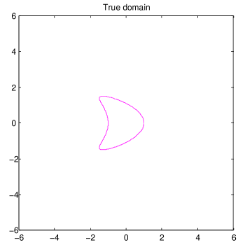
(a) Kite

(b) Peanut

Figure 1: Domains considered.

The synthetic scattering data are generated by the boundary integral equation method, i.e., $u^{\infty}_{p,q},\,p,q=1,2,\cdots,2m$, for $2m$ equidistantly distributed directions in $(0,2\pi]$. We first verify Theorem 2.1. Let $k=6$, $m=4$ and take the kite as an example. The MSR matrix $\mathbb{F}_{full}$ is $8\times 8$. The four block matrices are given as follows.

$$\mathbb{F}_{11} = \left(\begin{array}[]{cccc}-2.6282+1.8817i&0.1698+0.4158i&0.1657-0.2286i&1.0722-0.6313i\\ 0.0028-0.9694i&-2.5830+1.9160i&0.3264+0.1581i&-0.4424-0.9227i\\ -0.0740+0.7809i&0.2839-0.5024i&-2.4052+1.5689i&0.3264+0.1581i\\ 0.1929-0.5886i&0.2202+0.4858i&0.2839-0.5024i&-2.5830+1.9160i\\ \end{array}\right),$$

$$\mathbb{F}_{22} = \left(\begin{array}[]{cccccccc}-2.6282+1.8817i&0.0028-0.9694i&-0.0740+0.7809i&0.1929-0.5886i\\ 0.1698+0.4158i&-2.5830+1.9160i&0.2839-0.5024i&0.2202+0.4858i\\ 0.1657-0.2286i&0.3264+0.1581i&-2.4052+1.5689i&0.2839-0.5024i\\ 1.0722-0.6313i&-0.4424-0.9227i&0.3264+0.1581i&-2.5830+1.9160i\\ \end{array}\right),$$

$$\mathbb{F}_{12} = \left(\begin{array}[]{cccccccc}-0.5250+0.1132i&1.0722-0.6313i&0.1657-0.2286i&0.1698+0.4158i\\ 1.0722-0.6313i&-0.0050-0.3054i&0.1510+0.3285i&-0.5603-0.0594i\\ 0.1657-0.2286i&0.1510+0.3285i&-0.3128-0.5104i&-0.6526-1.3338i\\ 0.1698+0.4158i&-0.5603-0.0594i&-0.6526-1.3338i&-0.0441-0.9080i\\ \end{array}\right),$$

$$\mathbb{F}_{21} = \left(\begin{array}[]{cccccccc}-0.4473-0.3633i&0.1929-0.5886i&-0.0740+0.7809i&0.0028-0.9694i\\ 0.1929-0.5886i&-0.0441-0.9080i&-0.6526-1.3338i&-0.5603-0.0594i\\ -0.0740+0.7809i&-0.6526-1.3338i&-0.3128-0.5104i&0.1510+0.3285i\\ 0.0028-0.9694i&-0.5603-0.0594i&0.1510+0.3285i&-0.0050-0.3054i\\ \end{array}\right).$$

It is obvious that Theorem 2.1 holds:

$$\mathbb{F}_{11}=\mathbb{F}_{22}^{T},\quad\mathbb{F}_{12}=\mathbb{F}_{12}^{T}\quad\mbox{ and }\quad\mathbb{F}_{21}=\mathbb{F}_{21}^{T}.$$

In the rest of the section, we fix $k=6$ and divide $(0,2\pi)$ uniformly into $300\,(2m)$ directions. Assuming that the incident directions cover the full aperture, the observation directions only span a subset of $(0,2\pi)$. In particular, let $\hat{x}:=(\cos\phi,\sin\phi)$ with the observation angle $\phi$. Then we consider the measurements for three cases:

$$(1)\,\phi\in(0,\pi/2),\quad(2)\,\phi\in(0,2\pi/3),\quad\mbox{and}\quad(3)\,\phi\in(0,\pi).$$

Namely, we have the synthetic data $\mathbb{F}^{(l)}_{limit}$ for $l=1,\ldots,75$, $l=1,\ldots,100$, and $l=1,\ldots,150$, respectively. Then $\mathbb{F}^{(l)}_{limit}$ is perturbed by random noises

$$\mathbb{F}_{limit}^{(l),\delta}\,=\,\mathbb{F}_{limit}^{(l)}+\delta\|\mathbb{F}_{limit}^{(l)}\|\frac{R_{1}+R_{2}i}{\|R_{1}+R_{2}i\|},$$

where $R_{1}$ and $R_{2}$ are two matrixes containing pseudo-random values drawn from a normal distribution with mean zero and standard deviation one. The value of $\delta$ is the noise level, which is taken as $\delta=0.05$.

4.1 Data Recovery

Examples in this subsection are to test the validity of data recover algorithms proposed in Section 3. Given $\mathbb{F}_{limit}^{(l),\delta}$, the goal is to recover $\mathbb{F}_{full}^{\delta}$, the full-aperture MSR. We take the kite as the scatterer. The artificial domain $B$ is chosen to be a disc centered at the origin with radius $5$.

Figures 2-4 show the data reconstructions with different measurement apertures $(0,\pi/2),(0,2\pi/3),$ and $(0,\pi),$ respectively. We show the recovered data for the incident direction $d=(1,0)$, i.e., the first row of $\mathbb{F}_{full}^{\delta}$ in Figures 2$(a)$-4$(a)$. Only few data are well reconstructed. This is reasonable because both methods, MGF and MSLP, involve solving severely ill-posed integral equations. In particular, the symmetry does not apply in this case. Similar results with respective to $d=(0,1)$ are shown in Figures 2$(b)$-4$(b)$.

For incident angles in $[\pi,3\pi/2]$, we have obtained nearly exact far field pattern for all observation directions. In Figures 2$(c)(d)$-4$(c)(d)$ we show results for two incident directions $d=(-1,0)$ and $d=(0,-1)$. This further verify the symmetric structure of the multi-static response matrix.

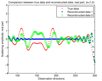
(a) $d=(1,0)$

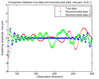
(b) $d=(0,1)$

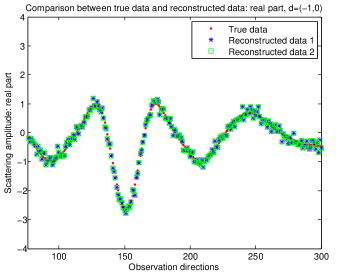
(c) $d=(-1,0)$

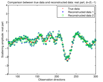
(d) $d=(0,-1)$

Figure 2: Exact data and recovered data with four different incident directions. Reconstructed data $1$ is obtained by MGF. Reconstructed data $2$ is obtained by MSLP. The measurements are taken with observation angles $\phi\in(0,\pi/2)$.

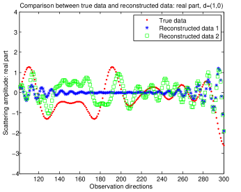
(a) $d=(1,0)$

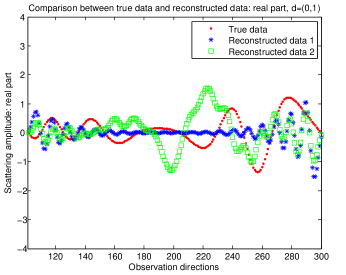
(b) $d=(0,1)$

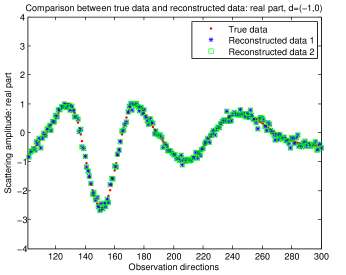
(c) $d=(-1,0)$

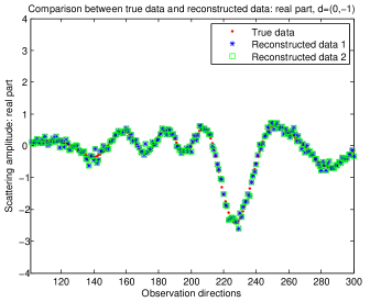
(d) $d=(0,-1)$

Figure 3: Exact data and recovered data with four different incident directions. Reconstructed data $1$ is obtained by MGF. Reconstructed data $2$ is obtained by MSLP. The measurements are taken with observation angles $\phi\in(0,2\pi/3)$.

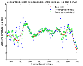
(a) $d=(1,0)$

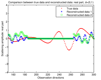
(b) $d=(0,1)$

(c) $d=(-1,0)$

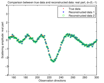
(d) $d=(0,-1)$

Figure 4: Exact data and recovered data with four different incident directions. Reconstructed data $1$ is obtained by MGF. Reconstructed data $2$ is obtained by MSLP. The measurements are taken with observation angles $\phi\in(0,\pi)$.

4.2 Applications in Sampling Methods

We first test the recovered data by a novel direct sampling method (DSM) proposed in [18], which uses an indicator functional defined as

$$I(z):=|\phi(z;-d)\mathbb{F}_{full}\phi^{T}(z;\hat{x})|^{2},$$ (4.7)

where $\phi(z;-d):=(e^{-ikz\cdot d_{1}},e^{-ikz\cdot d_{2}},\cdots,e^{-ikz\cdot d_{2m}})$ and $\phi(z;\hat{x}):=(e^{ikz\cdot\hat{x}_{1}},e^{ikz\cdot\hat{x}_{2}},\cdots,e^{ikz\cdot\hat{x}_{2m}})$. The indicator takes its maximum on or near the boundary of the scatterer. Consequently, the plot of the indicator can be used to reconstruct the scatterer.

This method can be modified to use only limited-aperture data by introducing

$$I_{limit}(z):=|\phi(z;-d)\mathbb{F}^{(l)}_{limit}\phi_{limit}^{T}(z;\hat{x})|^{2},$$ (4.8)

where $\phi_{limit}(z;\hat{x}):=(e^{ikz\cdot\hat{x}_{1}},e^{ikz\cdot\hat{x}_{2}},\cdots,e^{ikz\cdot\hat{x}_{l}})$ corresponds to the limited-aperture observation directions and $\mathbb{F}^{(l)}_{limit}$ is the limited-aperture data given by (2.17).

Denote by $\mathbb{F}^{(2)}_{full}$ and $\mathbb{F}^{(3)}_{full}$ the recovered full-aperture data using MGF and MSLP, respectively. We introduce the following indicator

$$I_{full}^{(ii)}(z):=|\phi(z;-d)\mathbb{F}^{(ii)}_{full}\phi^{T}(z;\hat{x})|^{2},\quad ii=2,3.$$ (4.9)

Alternatively, one can reconstruct the scatterer by $I_{full}^{(ii)}(z)$, $ii=2,3$ using recovered full-aperture data. As will seen shortly, the quality of the reconstructions indeed improves.

We used a grid $\mathcal{G}$ of $121\times 121$ equally spaced sampling points on some rectangle $[-6,6]\times[-6,6]$. For each point $z\in\mathcal{G}$, we compute the indicator functionals given in (4.8)-(4.9).

The typical feature for limited-aperture problems is that the concave part cannot be reconstructed if the the observation angles do not cover the concave part of the obstacle. A common criterion for judging the quality of a reconstruction method is whether the concave part of the obstacle can be successfully recovered. The resulting reconstructions by using the indicator functional $I_{limit}(z)$ with limited-aperture far field patterns are shown in Figures 5$(a)$, $(d)$, and $(g)$ for different observation apertures. Clearly, the quality improves with the increase of observation apertures. We also observe that the illuminated part is well constructed, but the shadow region is elongated down range.

As shown in the second and third columns of Figure 5, the reconstructions are indeed improved by using the data recover techniques. In particularly, the two wings of the kite appear and the shadow region is reconstructed very well. Considering the severe ill-posedness of the data reconstruction of an analytic function and the relative noise level $\delta=5\%$, the target reconstructions given in Figure 5 are satisfactory. Similar results are shown in Figures 6 for the peanut.

(a) $I_{limit}(z)$

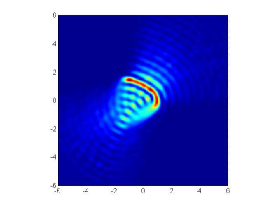
(b) $I^{(2)}_{full}(z)$

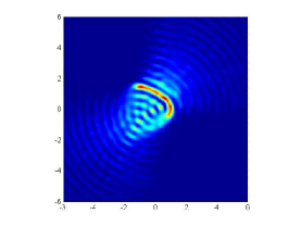
(c) $I^{(3)}_{full}(z)$

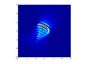
(d) $I_{limit}(z)$

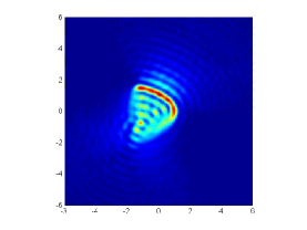
(e) $I^{(2)}_{full}(z)$

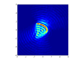
(f) $I^{(3)}_{full}(z)$

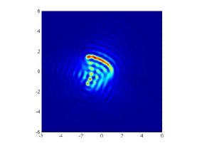
(g) $I_{limit}(z)$

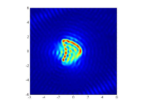
(h) $I^{(2)}_{full}(z)$

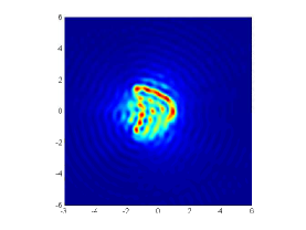
(i) $I^{(3)}_{full}(z)$

Figure 5: Shape and location reconstructions for kite by the direct sampling method. Top row: $\phi\in(0,\pi/2)$; Middle row: $\phi\in(0,2\pi/3)$; Bellow row: $\phi\in(0,\pi)$;.

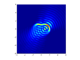
(a) $I_{limit}(z)$

(b) $I^{(2)}_{full}(z)$

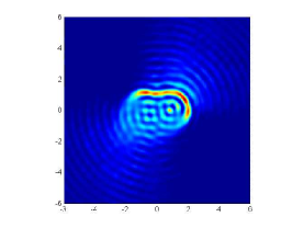
(c) $I^{(3)}_{full}(z)$

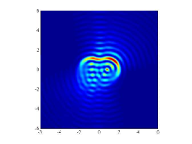
(d) $I_{limit}(z)$

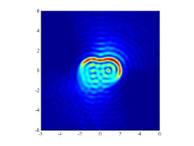
(e) $I^{(2)}_{full}(z)$

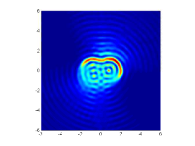
(f) $I^{(3)}_{full}(z)$

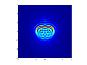
(g) $I_{limit}(z)$

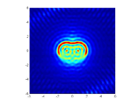
(h) $I^{(2)}_{full}(z)$

(i) $I^{(3)}_{full}(z)$

Figure 6: Shape and location reconstructions for peanut by the direct sampling method. Top row: $\phi\in(0,\pi/2)$; Middle row: $\phi\in(0,2\pi/3)$; Bellow row: $\phi\in(0,\pi)$;.

Finally, the recovered data is tested using the factorization method proposed by Kirsch [13, 14]. To our knowledge, the factorization method has not been established for limited aperture data. However, the factorization method applies using the recovered full-aperture data $\mathbb{F}^{(ii)}_{full}$, $ii=2,3$. Let $\{(\sigma_{n},\psi_{n}):n=1,...,2m\}$ represent the eigensystem of the matrix $F_{\sharp}$ given by

$$F_{\sharp}:=|\Re(\mathbb{F}^{(ii)}_{full})|+|\Im(\mathbb{F}^{(ii)}_{full})|.$$

We then define the indicator function

$$I^{(ii)}_{FM}(z):=\Biggl{[}\sum_{n=1}^{2m}\frac{|\phi_{z}^{*}\psi_{n}|^{2}}{|\sigma_{n}|}\Biggr{]}^{-1},\quad ii=2,3,$$

where $\phi_{z}=(e^{-ik\theta_{1}\cdot z},e^{-ik\theta_{2}\cdot z},\dots,e^{-ik\theta_{2m}\cdot z})^{\top}\in{\mathbb{C}}^{2m}$. Although the sum is finite, we expect the values of $I_{FM}(z)$ to be much smaller for the points belonging to $\Omega$ than for those lying in the exterior ${\mathbb{R}}^{2}\backslash\overline{D}$. Figure 7 shows the corresponding results with respect to measurements in $(0,\pi/2)$.

(a) $I^{(2)}_{FM}(z)$

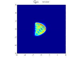
(b) $I^{(3)}_{FM}(z)$

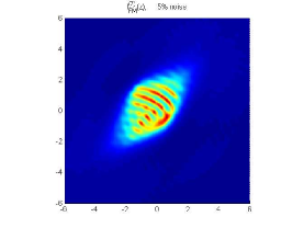
(c) $I^{(2)}_{FM}(z)$

(d) $I^{(3)}_{FM}(z)$

Figure 7: Reconstructions by the factorization method using recovered data. The observation angle $\phi\in(0,\pi/2)$. (a)-(b): without noise; (c)-(d): 5% noise.

5 Concluding Remarks

The limited-aperture problems arise in various areas of practical applications such as radar, remote sensing, geophysics, and nondestructive testing. It is well known that the illuminated part can be reconstructed well, while the shadow domain fails to be recovered. In this paper, based on the PDE theory for scattering problems, we introduce two techniques to recover the missing data that can not be measured directly. Using the recovered full-aperture data, a direct sampling method proposed in a recent paper [18] and the factorization method yield satisfactory reconstructions.

We conclude with some future works.

• The data recover techniques need to solve the ill-posed equations. We have used the Tikhonov regularization with regularization parameter $\alpha=10^{-2}$. The recovered data get worse as the direction moves further away from the measurable directions. A fast and stable method for solving the ill-posed equations is highly desired.

• Of greater practical importance would be the case that limited-aperture is not only for observation directions, but also the incident directions.

• It would be interesting and useful to consider the buried objects, where the measurements are only available in the upper half space.

References

• [1] C.Y. Ahn, K. Jeon, Y.K. Ma and W.K. Park, A study on the topological derivative-based imaging of thin electromagnetic inhomogeneities in limited-aperture problems, Inverse Problems 30, (2014), 105004.
• [2] D. Atkinson, Analytic extrapolations and inverse problems, Applied Inverse Problems (Lecture Notes in Physics 85) ed P. C. Sabatier, (Berlin: Springer), (1978), 111-121.
• [3] G. Bao and J. Liu, Numerical solution of inverse problems with multi-experimental limited aperture data, SIAM J.Sci.Comput. 25, (2003), 1102-1117.
• [4] F. Cakoni and D. Colton, A Qualitative Approach in Inverse Scattering Theory, AMS Vol.188, Springer-Verlag, 2014.
• [5] Y. Chen, Inverse scattering via Heisenberg’s uncertainty principle, Inverse Problems 13, (1997), 253-282.
• [6] J. Chen, Z. Chen and G. Huang, Reverse time migration for extended obstacles: acoustic waves, Inverse Problems 29, (2013), 085005.
• [7] D. Colton and A. Kirsch, A simple method for solving inverse scattering problems in the resonance region. Inverse Problems 12 (1996), 383-393.
• [8] D. Colton and R. Kress, Inverse Acoustic and Electromagnetic Scattering Theory (Third Edition), Springer, 2013.
• [9] D. Colton and P. Monk, A novel method for solving the inverse scattering problem for time-harmonic acoustic waves in the resonance region, SIAM J.Appl.Math, 45, (1985), 1039-1053.
• [10] M. Ikehata, E. Niemi and S. Siltanen, Inverse obstacle scattering with limited-aperture data, Inverse Probl. Imaging 1, (2012), 77–94.
• [11] K. Ito, B. Jin, and J. Zou, A direct sampling method to an inverse medium scattering problem, Inverse Problems 28, (2012), 025003.
• [12] R. L. OCHS, JR., The limited aperture problem of inverse acoustic scattering: Dirichlet boundary conditions, SIAM J. Appl. Math. 47(6), (1987), 1320–1341.
• [13] A. Kirsch, Charaterization of the shape of a scattering obstacle using the spectral data of the far field operator, Inverse Problems 14, (1998), 1489–1512.
• [14] A. Kirsch and N. Grinberg, The Factorization Method for Inverse Problems, Oxford University Press, 2008.
• [15] A. Kirsch and R. Kress, An optimization method in inverse acoustic scattering, In Brebbia et al., editor, Boundary Elements, IX, Vol3, Fluid Flow and Potential Applications, Springer, (1987), 3-18.
• [16] A. Kirsch and X. Liu. A modification of the factorization method for the classical acoustic inverse scattering problems, Inverse Problems 30, (2014), 035013.
• [17] J. Li, P. Li, H. Liu and X. Liu, Recovering multiscale buried anomalies in a two-layered medium, Inverse Problems 31, (2015), 105006.
• [18] X. Liu, A novel sampling method for multiple multiscale targets from scattering amplitudes at a fixed frequency, Inverse Problems 33, (2017), 085011.
• [19] X. Liu and B. Zhang, Recent progress on the factorization method for inverse acoustic scattering problems (in Chinese), Sci. Sin. Math, 45, (2015), 873-890.
• [20] R.D. Mager and N. Bleistein, An approach to the limited aperture problem of physical optics far field inverse scattering, Tech. Report Ms-R-7704, University of Denver, Denver, CO, 1977.
• [21] R.D. Mager and N. Bleistein, An examination of the limited aperture problem of physical optics inverse scattering IEEE Trans, Antennas Propag. 26, (1978) 695–699.
• [22] W. Mclean, Strongly Elliptic Systems and Boundary Integral Equation, Cambridge University Press, Cambridge, 2000.
• [23] R. Potthast, A study on orthogonality sampling, Inverse Problems 26, (2010), 074075.
• [24] J. Sun, An eigenvalue method using multiple frequency data for inverse scattering problems, Inverse Problems 28, (2012), 025012.
• [25] A. Zinn, On an optimisation method for the full- and limited-amperture problem in inverse acoustic scattering for a sound-soft obstacle, Inverse Problems 5, (1989), 239-253.