A Review of Self-Exciting Spatio-Temporal Point Processes and Their Applications

Abstract

Self-exciting spatio-temporal point process models predict the rate of events as a function of space, time, and the previous history of events. These models naturally capture triggering and clustering behavior, and have been widely used in fields where spatio-temporal clustering of events is observed, such as earthquake modeling, infectious disease, and crime. In the past several decades, advances have been made in estimation, inference, simulation, and diagnostic tools for self-exciting point process models. In this review, I describe the basic theory, survey related estimation and inference techniques from each field, highlight several key applications, and suggest directions for future research.

1 Introduction

Self-exciting spatio-temporal point processes, an extension of temporal Hawkes processes, model events whose rate depends on the past history of the process. These have proven useful in a wide range of fields: seismological models of earthquakes and aftershocks, criminological models of the dynamics of crime, epidemiological forecasting of the incidence of disease, and many others. In each field, the spatio-temporal distribution of events is of scientific and practical interest, both for prediction of new events and to improve understanding of the process generating the events. We may have a range of statistical questions about the process: does the rate of events vary in space and time? What spatial or temporal covariates may be related to the rate of events? Do events trigger other events, and if so, how are the triggered events distributed in space and time?

Regression is a natural first approach to answer these questions. By dividing space into cells, either on a grid or following natural or political boundaries, and dividing the observed time window into short discrete intervals, we can aggregate events and regress the number of events observed in a given cell and interval against spatial and temporal covariates, prior counts of events in neighboring cells, and so on. This approach has been widely used in applications. However, it suffers several disadvantages: most notably, the Modifiable Areal Unit Problem means that estimated regression coefficients and their variances may vary widely depending on the boundaries or grids chosen for aggregation, and there is no natural “correct” choice (Fotheringham and Wong, 1991).

Instead, we can model the rate of occurrence of events directly, without aggregation, by treating the data as arising from a point process. If the questions of scientific interest are purely spatial, the events can be analyzed using methods for spatial point processes (Diggle, 2014), and their times can be ignored. If time is important, descriptive statistics for the first- and second-order properties of a point process, such as the average intensity and clustering behavior, can also be extended to spatio-temporal point processes (Diggle, 2014, chapter 11).

When descriptive statistics are not enough to understand the full dynamics of the point process, we can use spatio-temporal point process models. These models estimate an intensity function which predicts the rate of events at any spatial location $s$ and time $t$. The simplest case is the homogeneous Poisson process, where the intensity is constant in space and time. An example of a more flexible inhomogeneous model is the log-Gaussian Cox process, reviewed by Diggle et al. (2013), in which the log intensity is assumed to be drawn from a Gaussian process. With a suitable choice of spatio-temporal correlation function, the underlying Gaussian process can be estimated, though this can be computationally challenging.

Cluster processes, which directly model clustering behavior, split the process in two: cluster centers, generally unobserved, are drawn from a parent process, and each cluster center begets an offspring process centered at the parent (Daley and Vere-Jones, 2003, Section 6.3). The observed process is the superposition of the offspring processes. A common case is the Poisson cluster process, in which cluster centers are drawn from a Poisson process; special cases include the Neyman–Scott process, in which offspring are also drawn from a Poisson process, and the Matérn cluster process, in which offspring are drawn uniformly from disks centered at the cluster centers. Common cluster processes, other spatio-temporal models, and descriptive statistics were reviewed by González et al. (2016).

In this review, I will focus on self-exciting spatio-temporal point process models, where the rate of events at time $t$ may depend on the history of events at times preceding $t$, allowing events to trigger new events. These models are characterized by a conditional intensity function, discussed in Section 2, which is conditioned on the past history of the process, and has a direct representation as a form of cluster process. Parametrization by the conditional intensity function has allowed a wide range of self-exciting models incorporating features like seasonality, spatial and temporal covariates, and inhomogeneous background event rates to be developed across a range of application areas.

Dependence on the past history of the process is not captured by log-Gaussian Cox processes or spatial regression, but can be of great interest in some applications: the greatest development of self-exciting models has been in seismology, where prediction of aftershocks triggered by large earthquakes is important for forecasting and early warning. However, literature on theory, estimation, and inference for self-exciting models has largely been isolated within each application, so the purpose of this review is to synthesize these developments and place them in context, drawing connections between each application and paving the way for new uses.

Self-exciting models can be estimated using standard maximum likelihood approaches, discussed in Section 3.1 below. Once a self-exciting model is estimated, we are able to answer a range of scientifically interesting questions about the dynamics of their generating processes. Section 3.2 reviews stochastic declustering methods, which attribute events to the prior events which triggered them, or to the underlying background process, using the estimated form of the triggering function. Section 3.3 then introduces algorithms to efficiently simulate new data, and Section 3.4 discusses methods for estimating model standard errors and confidence intervals. Bayesian approaches are discussed in Section 3.5, and general model-selection and diagnostic techniques in Section 3.6.

Finally, Section 4 introduces three major application areas of self-exciting spatio-temporal point processes: earthquake forecasting, models of the dynamics of crime, and models of infectious disease. These demonstrate the utility of self-exciting models and illustrate each of the techniques described in Section 3. Section 4.4 introduces a further extension of self-exciting point processes, extending them from spatio-temporal settings to applications involving events occurring on networks.

2 Self-Exciting Spatio-Temporal Point Processes

2.1 Hawkes Processes

Consider a temporal simple point process of event times $t_{i}\in[0,T)$, such that $t_{i}<t_{i+1}$, and a right-continuous counting measure $N(A)$, defined as the number of events occurring at times $t\in A$. Associated with the process is the history ${\cal H}_{t}$ of all events up to time $t$. We may characterize the process by its conditional intensity, defined as

$$\lambda(t\mid{\cal H}_{t})=\lim_{\Delta t\to 0}\frac{\operatorname{\mathbb{E}}\left[N\left([t,t+\Delta t)\right)\mid{\cal H}_{t}\right]}{\Delta t}.$$

The self-exciting point process model was introduced for temporal point processes by Hawkes (1971). Self-exciting processes can be defined in terms of a conditional intensity function in the equivalent forms

$$\lambda(t\mid{\cal H}_{t}) =\nu+\int_{0}^{t}g(t-u)\operatorname{d\!}N(u)$$

$$=\nu+\sum_{i\mathrel{\mathop{\mathchar 58\relax}}t_{i}<t}g(t-t_{i}),$$

where $\nu$ is a constant background rate of events and $g$ is the triggering function which determines the form of the self-excitation. The process is called “self-exciting” because the current conditional intensity is determined by the past history ${\cal H}_{t}$ of the process. Depending on the form chosen for the triggering function $g$, the process may depend only on the recent history (if $g$ decays rapidly) or may have longer term effects. Typically, because $\lambda(t\mid{\cal H}_{t})\geq 0$, we require $g(u)\geq 0$ for $u\geq 0$ and $g(u)=0$ for $u<0$.

Hawkes processes have been put to many uses in a range of fields, modeling financial transactions (Bauwens and Hautsch, 2009; Bacry, Mastromatteo and Muzy, 2015), neuron activity (Johnson, 1996), terrorist attacks (Porter and White, 2012), and a wide range of other processes. They are particularly useful in processes that exhibit clustering: Hawkes and Oakes (1974) demonstrated that any stationary self-exciting point process with finite intensity may be interpreted as a Poisson cluster process. The events may be partitioned into disjoint processes: a background process of cluster centers $N_{c}(t)$, which is simply a Poisson process with rate $\nu$, and separate offspring processes of triggered events inside each cluster, whose intensities are determined by $g$. Each triggered event may then trigger further events. Fig. 1 illustrates this separation. The number of offspring of each event is drawn from a Poisson distribution with mean

$$m=\int_{0}^{\infty}g(t)\operatorname{d\!}t.$$

Provided $m<1$, cluster sizes are almost surely finite, as each generation of offspring follows a geometric progression, with expected total cluster size of $1/(1-m)$ including the initial background event. This partitioning also permits other useful results, such as an integral equation for the distribution of the length of time between the first and last events of a cluster (Hawkes and Oakes, 1974, Theorem 5).

Figure 1: At top, a hypothetical observed self-exciting point process of events from $t=0$ to $t=10$. Below, the separation of that process into a background process and two generations of offspring processes. The arrows indicate the cluster relationships of which events were triggered by which preceding events; solid circles are background events, and open circles and squares are triggered events. At bottom, the combined process with generation indicated by shapes and shading. This cluster structure is not directly observed, though it may be inferred with the methods of Section 3.2.

2.2 Spatio-Temporal Form

Spatio-temporal models extend the conditional intensity function to predict the rate of events at locations $s\in X\subseteq\mathbb{R}^{d}$ and times $t\in[0,T)$. The function is defined in the analogous way to temporal Hawkes processes:

$$\lambda(s,t\mid{\cal H}_{t})=\lim_{\Delta s,\Delta t\to 0}\frac{\operatorname{\mathbb{E}}\left[N\left(B(s,\Delta s)\times[t,t+\Delta t)\right)\mid{\cal H}_{t}\right]}{|B(s,\Delta s)|\Delta t},$$ (1)

where $N(A)$ is again the counting measure of events over the set $A\subseteq X\times[0,T)$ and $|B(s,\Delta s)|$ is the Lebesgue measure of the ball $B(s,\Delta s)$ with radius $\Delta s$.

A self-exciting spatio-temporal point process is one whose conditional intensity is of the form

$$\lambda(s,t\mid{\cal H}_{t})=\mu(s)+\sum_{i\mathrel{\mathop{\mathchar 58\relax}}t_{i}<t}g(s-s_{i},t-t_{i}),$$ (2)

where $\{s_{1},s_{2},\dots,s_{n}\}$ denotes the observed sequence of locations of events and $\{t_{1},t_{2},\dots,s_{n}\}$ the observed times of these events. Generally the triggering function $g$ is nonnegative, and is often a kernel function or power law decay function; often, for simplicity, it is taken to be separable in space and time, so that $g(s-s_{i},t-t_{i})=f(s-s_{i})h(t-t_{i})$, similar to covariance functions in other spatio-temporal models (Cressie and Wikle, 2011, Section 6.1). Sometimes a general nonparametric form is used, as in the model described in Section 3.2.3.

For ease of notation, the explicit conditioning on the past history ${\cal H}_{t}$ will be omitted for the rest of this review, and should be read as implied for all self-exciting conditional intensities.

As with Hawkes processes, spatio-temporal self-exciting processes can be treated as Poisson cluster processes, with the mean number of offspring

$$m=\int_{X}\int_{0}^{T}g(s,t)\operatorname{d\!}t\operatorname{d\!}s.$$ (3)

The triggering function $g$, centered at the triggering event, is the intensity function for the offspring process. Properly normalized, it induces a probability distribution for the location and times of the offspring events. The cluster process representation will prove crucial to the efficient estimation and simulation of self-exciting processes, and the estimation of the cluster structure of the process will be the focus of Section 3.2.

To illustrate the cluster process behavior of spatio-temporal self-exciting processes, Fig. 2 compares a simulated realization of a spatio-temporal inhomogeneous Poisson process against a self-exciting process using the same Poisson process realization as its background process. The self-exciting process, simulated using a Gaussian triggering function with a short bandwidth, shows clusters (of expected total cluster size 4) emerging from the Poisson process. The simulation was performed using Algorithm 5, to be discussed in Section 3.3, which directly uses the cluster process representation to make simulation more efficient.

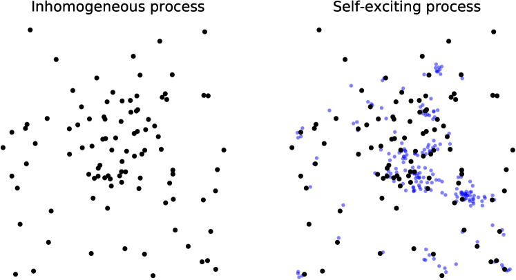
Figure 2: At left, a realization of an inhomogeneous Poisson process, in which the intensity is higher inside a central square and lower outside. At right, a self-exciting process with average total cluster size of 4, using the inhomogeneous Poisson process as the background process. Excited events are shown in blue. The cluster structure of the process is clearly visible, with clumps emerging from the self-excitation.

2.3 Marks

Point processes may be marked if features of events beyond their time or location are also observed (Daley and Vere-Jones, 2003, Section 6.4). For example, if earthquakes are treated as a spatiotemporal point process of epicenter locations and times, the magnitude of each earthquake is an additional observed variable which is an important part of the process: the number and distribution of aftershocks may depend upon it. A marked point process is hence a point process of events $\{(s_{i},t_{i},\kappa_{i})\}$, where $s_{i}\in X\subseteq\mathbb{R}^{d}$, $t_{i}\in[0,T)$, and $\kappa_{i}\in{\cal K}$, where ${\cal K}$ is the mark space (e.g. the space of earthquake magnitudes). A special case is the multivariate point process, in which the mark space is a finite set $\{1,\dots,m\}$ for a finite integer $m$. Often the mark in a multivariate point process indicates the type of each event, such as the type of crime reported.

Marks can have several useful properties. A process has independent marks if, given the locations and times $\{(s_{i},t_{i})\}$ of events, the marks are mutually independent of each other, and the distribution of $\kappa_{i}$ depends only on $(s_{i},t_{i})$. Separately, a process has unpredictable marks if $\kappa_{i}$ is independent of all locations and marks $\{(s_{j},t_{j},\kappa_{j})\}$ of previous events ($t_{j}<t_{i}$).

A marked point process has a ground process, the point process of event locations and times without their corresponding marks. Using the ground process conditional intensity $\lambda_{g}(s,t)$, we can write the marked point process’s conditional intensity function as

$$\lambda(s,t,\kappa)=\lambda_{g}(s,t)f(\kappa\mid s,t),$$ (4)

where $f(\kappa\mid s,t)$ is the conditional density of the mark at time $t$ and location $s$ given the history of the process up to $t$. In general, the ground process may depend on the past history of marks as well as the past history of event locations and times. For simplicity of notation, the following sections will largely consider point processes without marks, except where noted, but most methods apply to marked and unmarked processes alike.

2.4 Log-Likelihood

The likelihood function for a particular parametric conditional intensity model is not immediately obvious: given the potentially complex dependence caused by self-excitation, even the distribution of the total number of events observed in a time interval is difficult to obtain, and the spatial distributions of this varying number of events must also be accounted for. Instead, for a realization of $n$ points from a point process, we start with its Janossy density (Daley and Vere-Jones, 2003, Section 5.3). For a temporal point process, where a realization is the set of event times $\{t_{1},t_{2},\dots,t_{n}\}$ in a set $T$, the Janossy density is defined by the Janossy measure $J_{n}$,

$$J_{n}(A_{1}\times\cdots\times A_{n})=n!p_{n}\Pi_{n}^{\text{sym}}(A_{1}\times\cdots\times A_{n}),$$

where the total number of events is $n$, $p_{n}$ is the probability of a realization of the process containing exactly $n$ events, $(A_{1},\dots,A_{n})$ is a partition of $T$ where $A_{i}$ represents possible times for event $i$, and $\Pi_{n}^{\text{sym}}(\cdot)$ is a symmetric probability measure determining the joint distribution of the times of events in the process, given there are $n$ total events. The Janossy measure is not a probability measure: it represents the sum of the probabilities of all $n!$ permutations of $n$ points. It is nonetheless useful, as its density $j_{n}(t_{1},\dots,t_{n})\operatorname{d\!}t_{1}\cdots\operatorname{d\!}t_{n}$ has an intuitive interpretation as the probability that there are exactly $n$ events in the process, one in each of the $n$ infinitesimal intervals $(t_{i},t_{i}+\operatorname{d\!}t_{i})$.

This interpretation connects the Janossy density to the likelihood function, which can be written as (Daley and Vere-Jones, 2003, Definition 7.1.II)

$$L_{T}(t_{1},\dots,t_{n})=j_{n}(t_{1},\dots,t_{n}\mid T)$$ (5)

for a process on a bounded Borel set of times $T$; for simplicity in the rest of this section, we’ll consider times in the interval $[0,T)$. Here $j_{n}(t_{1},\dots,t_{n}\mid T)$ denotes the local Janossy density, interpreted as the probability that there are exactly $n$ events in the process before time $T$, one in each of the infinitesimal intervals.

The likelihood can be rewritten in terms of the conditional intensity function, which is usually easier to define than the Janossy density, by connection with survival and hazard functions. Consider the conditional survivor functions $S_{k}(t\mid t_{1},\dots,t_{k-1})=\Pr(t_{k}>t\mid t_{1},\dots,t_{k-1})$. Using these functions and the conditional probability densities $p_{k}(t\mid t_{1},\dots,t_{k-1})$ of event times, we can write the Janossy density recursively as

$$\begin{split}j_{n}(t_{1},\dots,t_{n}\mid T)={}&p_{1}(t_{1})p_{2}(t_{2}\mid t_{1})\cdots p_{n}(t_{n}\mid t_{1},\dots,t_{n-1})\times{}\\ &S_{n+1}(T\mid t_{1},\dots,t_{n}).\end{split}$$ (6)

Additionally, we may define the hazard functions

$$\begin{split}h_{k}(t\mid t_{1},\dots,t_{k_{1}})&=\frac{p_{k}(t\mid t_{1},\dots,t_{k-1})}{S_{k}(t\mid t_{1},\dots,t_{k-1})}\\ &=-\mathinner{\dfrac{\operatorname{d\!}{}\log S_{k}(t\mid t_{1},\dots,t_{k-1})}{\operatorname{d\!}{t}}}.\end{split}$$ (7)

The hazard function has a natural interpretation as the conditional instantaneous event rate—which means the conditional intensity $\lambda(t)$ can be written directly in terms of the hazard functions:

$$\lambda(t)=\begin{cases}h_{1}(t)&0<t<t_{1}\\ h_{k}(t\mid t_{1},\dots,t_{k-1})&t_{k-1}<t\leq t_{k},k\geq 2.\end{cases}$$

This allows us to write the likelihood from eq. (5) in terms of the conditional intensity function instead of the Janossy density. Observe that from eq. (7) we may write

$$S_{k}(t\mid t_{1},\dots,t_{k-1})=\exp\left(-\int_{t_{k-1}}^{t}h_{k}(u\mid t_{1},\dots,t_{k-1})\operatorname{d\!}u\right)$$

Substituting eq. (7) into eq. (6), replacing the hazard function with the conditional intensity, and combining terms leads to the likelihood, for a complete parameter vector $\Theta$, of (Daley and Vere-Jones, 2003, Proposition 7.2.III)

$$L(\Theta)=\left[\prod_{i=1}^{n}\lambda(t_{i})\right]\exp\left(-\int_{0}^{T}\lambda(t)\operatorname{d\!}t\right).$$

By treating spatial locations as marks, we may obtain extend this argument to spatio-temporal processes and obtain the log-likelihood (Daley and Vere-Jones, 2003, Proposition 7.3.III):

$$\ell(\Theta)=\sum_{i=1}^{n}\log\left(\lambda(s_{i},t_{i})\right)-\int_{0}^{T}\int_{X}\lambda(s,t)\operatorname{d\!}s\operatorname{d\!}t,$$ (8)

where $X$ is the spatial domain of the observations. For spatio-temporal marked point processes with intensity defined as in eq. (4), the log-likelihood is written in terms of the ground process, and has an extra mark term (Daley and Vere-Jones, 2003, Proposition 7.3.III):

$$\begin{split}\ell(\Theta)={}&\sum_{i=1}^{n}\log\left(\lambda_{g}(s_{i},t_{i})\right)+\sum_{i=1}^{n}\log\left(f(m_{i}\mid s_{i},t_{i})\right)\\ &{}-\int_{0}^{T}\int_{X}\lambda_{g}(s,t)\operatorname{d\!}s\operatorname{d\!}t.\end{split}$$

In unmarked processes, the first term in eq. (8) is easy to calculate, assuming the conditional intensity is straightforward, but the second term can require computationally expensive numerical integration methods.

There are several approaches to evaluate this integral. The spatial domain $X$ can be arbitrary—e.g. a polygon defining the boundaries of a city—so Meyer, Elias and Höhle (2012) (see Section 4.3) used two-dimensional numeric integration via cubature, as part of a numerical maximization routine. This requires an expensive numeric integration at every step of the numerical maximization, making the procedure unwieldy.

Schoenberg (2013) observed that, for some conditional intensities, it may be much easier to analytically integrate over $\mathbb{R}^{2}$ instead of an arbitrary $X$. Hence the approximation

$$\int_{0}^{T}\int_{X}\lambda(s,t)\operatorname{d\!}s\operatorname{d\!}t\leq\int_{0}^{\infty}\int_{\mathbb{R}^{2}}\lambda(s,t)\operatorname{d\!}s\operatorname{d\!}t$$

may reduce the integral to a form which may be evaluated directly. The approximation is exact when the effect of self-excitation is contained entirely within $X$ and before $t=T$, and overestimates otherwise; because overestimation decreases the calculated log-likelihood, Schoenberg argued that likelihood maximization will avoid parameter values where overestimation is large. Lippiello et al. (2014) argued that the temporal approximation biases parameter estimates more than the spatial one, and advocated only approximating $X$ by $\mathbb{R}^{2}$. This approximation was used by Mohler (2014), discussed in Section 4.2. Lippiello et al. (2014) also proposed a more accurate spatial approximation method based on a transformation of the triggering function to polar coordinates.

3 Estimation and Inference

Suppose now we have observed a realization of a self-exciting point process, with event locations $\{s_{1},s_{2},\dots,s_{n}\}$ and times $\{t_{1},t_{2},\dots,t_{n}\}$ over a spatial region $X$ and temporal window $[0,T)$. We have a model for the conditional intensity function and would like to be able to estimate its parameters, perform inference, and simulate new data if needed. This section discusses common approaches to these problems in the literature, focusing largely on maximum likelihood estimation, though with a brief discussion of Bayesian approaches in Section 3.5.

Fitting conditional intensity functions is not the only way to approach spatio-temporal point processes; there is also extensive literature which primarily uses descriptive statistics, such as first and second order moments of the process. I will not delve into this literature here, as it is less useful for understanding self-exciting processes; nonetheless, Vere-Jones (2009) gives a brief review, and more thorough treatments are available from González et al. (2016) and Diggle (2014).

3.1 Maximum Likelihood

Self-exciting point process models are most commonly fit using maximum likelihood. This is usually impossible to perform analytically: the form of the log-likelihood in eq. (8) involves a sum of logarithms of conditional intensities, which themselves involve sums over previous points, making analytical maximization intractable. Numerical evaluation of the intensity takes $O(n^{2})$ time, and the log-likelihood can be nearly flat in large regions of the parameter space, causing problems for numerical maximization algorithms and making convergence extremely slow; in some examples explored by Veen and Schoenberg (2008), numerical maximization may fail to converge altogether. Nonetheless, for small datasets where the log-likelihood is computationally tractable to evaluate, numerical maximization is often used.

Alternately, Veen and Schoenberg (2008) showed the likelihood can be maximized with the expectation maximization (EM) algorithm (Dempster, Laird and Rubin, 1977; McLachlan and Krishnan, 2008) by introducing a latent quantity $u_{i}$ for each event $i$, which indicates whether the event came from the background ($u_{i}=0$) or was triggered by a previous event $j$ ($u_{i}=j$). This follows naturally from the cluster process representation discussed in Sections 2.1 and 2.2: if $u_{i}=0$, event $i$ is a cluster center, and otherwise it is the offspring (directly or indirectly) of a cluster center.

Veen and Schoenberg (2008) derived the complete-data log-likelihood for a specific earthquake clustering model. More generally, consider a model of the form given in eq. (2). If the branching structure $u_{i}$ is assumed to be known, the complete-data log-likelihood for a parameter vector $\Theta$ can be written as

$$\begin{split}\ell_{c}(\Theta)={}&\sum_{i=1}^{n}\operatorname{\mathbb{I}}(u_{i}=0)\log\left(\mu(s_{i})\right)\\ &{}+\sum_{i=1}^{n}\sum_{j=1}^{n}\operatorname{\mathbb{I}}(u_{i}=j)\log\left(g(s_{i}-s_{j},t_{i}-t_{j})\right)\\ &{}-\int_{0}^{T}\int_{X}\lambda(s,t)\operatorname{d\!}s\operatorname{d\!}t,\end{split}$$

where $\operatorname{\mathbb{I}}(\cdot)$ is the indicator function, which is one when its argument is true and zero otherwise. The branching structure dramatically simplifies the log-likelihood, as each event’s intensity comes only from its trigger (the background or a previous event); this is analogous to the common EM approach to mixture models, where the latent variables indicate the underlying distribution from which each point came.

To complete the E step, we take the expectation of $\ell_{c}(\Theta)$. This requires estimating the triggering probabilities $\Pr(u_{i}=j)=\operatorname{\mathbb{E}}[\operatorname{\mathbb{I}}(u_{i}=j)]$ for all $i$, $j$, based on the current parameter values $\hat{\Theta}$ for this iteration. We can calculate these probabilities as

$$\Pr(u_{i}=j) =\begin{cases}\frac{g(s_{i}-s_{j},t_{i}-t_{j})}{\lambda(s_{i},t_{i})}&t_{j}<t_{i}\\ 0&t_{j}\geq t_{i}\end{cases}$$ (9)

$$\Pr(u_{i}=0) =1-\sum_{j=1}^{i-1}P(u_{i}=j)=\frac{\mu(s_{i})}{\lambda(s_{i},t_{i})}.$$ (10)

This leads to the expected complete-data log-likelihood

$$\begin{split}\operatorname{\mathbb{E}}[\ell_{c}(\Theta)]={}&\sum_{i=1}^{n}\Pr(u_{i}=0)\log\left(\mu(s_{i})\right)\\ &{}+\sum_{i=1}^{n}\sum_{j=1}^{n}\Pr(u_{i}=j)\log\left(g(s_{i}-s_{j},t_{i}-t_{j})\right)\\ &{}-\int_{0}^{T}\int_{X}\lambda(s,t)\operatorname{d\!}s\operatorname{d\!}t,\end{split}$$

which is much easier to analytically or numerically maximize with respect to each parameter in the M step. Once new parameter estimates are found, the procedure returns to the E step, estimating new triggering probabilities, and repeats until the log-likelihood converges, or until the estimated parameter values change by less than some pre-specified tolerance.

The EM algorithm has several advantages over other numerical maximization methods. Introducing the branching structure avoids the typical numerical issues encountered by other maximization algorithms, making the maximization at each iteration much easier, and the triggering probabilities also have a dual use in stochastic declustering algorithms, discussed in the next section.

One important warning must be kept in mind, however. If we have observed only data in the region $X$ and time interval $[0,T)$, but the underlying process extends outside this region and time, our parameter estimates will be biased by boundary effects (Zhuang, Ogata and Vere-Jones, 2004). Unobserved events just outside $X$ or before $t=0$ can produce observed offspring which may be incorrectly attributed to the background process, and observed events near the boundary can produce offspring outside it, leading estimates of the mean number of offspring $m$ (see eq. (3)) to be biased downward. Boundary effects can also bias the estimated intensity $\lambda(s,t)$ in ways analogous to the bias experienced in kernel density estimation (Cowling and Hall, 1996), but these effects are not well characterized for common self-exciting models.

3.2 Stochastic Declustering

For some types of self-exciting point processes, the background event rate $\mu(s)$ is fit nonparametrically from the observed data, for example by kernel density estimation or using splines (Ogata and Katsura, 1988). This could be fit by maximum likelihood—Mohler (2014) fit the background as a weighted kernel density via maximum likelihood, for example—but in some cases, we would like to estimate $\mu(s)$ using events from the background process only, and not using events which were triggered by those events. We may also want to analyze the background process intensity separately from the triggered events, since the background process may have an important physical interpretation. This requires a procedure which can separate background events from triggered events, as illustrated in Fig. 1: stochastic declustering.

3.2.1 Model-Based Stochastic Declustering.

This version of stochastic declustering, introduced by Zhuang, Ogata and Vere-Jones (2002), assumes that the triggering function $g$ has a parametric form, but that the background $\mu(s)$ should be estimated nonparametrically from only background events. Estimating the background requires determining whether each event was triggered by the background, but to do so requires $g$, so the procedure is iterative, starting with initial parameter values and alternately updating the background estimate and $g$ until convergence.

Consider the total spatial intensity function, defined as (Zhuang, Ogata and Vere-Jones, 2002)

$$m_{1}(s)=\lim_{T\to\infty}\frac{1}{T}\int_{0}^{T}\lambda(s,t)\operatorname{d\!}t,$$ (11)

where $T$ is the length of the observation period. The function $m_{1}(s)$ does not require declustering to estimate, since it sums over all events, including triggered events; by replacing the limit in eq. (11) with a finite-data approximation and substituting in eq. (2), we obtain

$$m_{1}(s) \approx\frac{1}{T}\int_{0}^{T}\mu(s)+\sum_{i\mathrel{\mathop{\mathchar 58\relax}}t_{i}<t}g(s-s_{i},t-t_{i})\operatorname{d\!}t$$

$$=\mu(s)+\frac{1}{T}\int_{0}^{T}\sum_{i\mathrel{\mathop{\mathchar 58\relax}}t_{i}<t}g(s-s_{i},t-t_{i})\operatorname{d\!}t.$$

We hence obtain the relation

$$\mu(s)\approx m_{1}(s)-\frac{1}{T}\sum_{i\mathrel{\mathop{\mathchar 58\relax}}t_{i}<t}\int_{0}^{T}g(s-s_{i},t-t_{i})\operatorname{d\!}t.$$ (12)

We can now use a suitable nonparametric technique, such as kernel density estimation, to form $\hat{m}_{1}(s)$:

$$\hat{m}_{1}(s)=\frac{1}{T}\sum_{i=1}^{n}k(s-s_{i}),$$

where $k$ is a kernel function. It may also be desirable to estimate the second term on the right-hand side of eq. (12), denoted $\gamma(s)$, the same way. To do so, we use the same latent quantity $u_{i}$ defined and estimated in Section 3.1. We can estimate the cluster process by, for example, a weighted kernel density estimate, using

$$\hat{\gamma}(s)=\frac{1}{T}\sum_{i=1}^{n}\Pr(u_{i}\neq 0)k(s-s_{i}).$$

This leads to the estimator

$$\begin{split}\hat{\mu}(s)&=\hat{m}_{1}(s)-\hat{\gamma}(s)\\ &=\frac{1}{T}\sum_{i=1}^{n}(1-\Pr(u_{i}\neq 0))k(s-s_{i}).\end{split}$$ (13)

We now need to iteratively estimate parameters of the triggering function $g$. Provided these can be found by maximum likelihood, Zhuang, Ogata and Vere-Jones (2002) suggested the following algorithm:

Algorithm 1.

Let $\hat{\mu}(s)=1$ initially.

1. Using maximum likelihood (see Section 3.1), fit the parameters of the conditional intensity function

   $$\lambda(s,t)=\hat{\mu}(s)+\sum_{i\mathrel{\mathop{\mathchar 58\relax}}t_{i}<t}g(s-s_{i},t-t_{i}).$$

2. Calculate $\Pr(u_{i}\neq 0)$ for all $i$ using the parameters found in step 1 and eq. (10).

3. Using the new branching probabilities, form a new $\hat{\mu}^{*}(s)$ using eq. (13).

4. If $\max_{s}|\hat{\mu}(s)-\hat{\mu}^{*}(s)|>\epsilon$, for a pre-chosen tolerance $\epsilon>0$, return to step 1. Otherwise, terminate the algorithm.

We can now perform stochastic declustering by thinning the process. With the final estimated $\hat{\mu}(s)$, we recalculate $\Pr(u_{i}\neq 0)$ and keep each event with probability $1-\Pr(u_{i}\neq 0)$; the rest of the events are considered triggered events and deleted. We are left with those identified as background events.

In the original implementation of this algorithm, Zhuang, Ogata and Vere-Jones (2002) used an adaptive kernel function $k$ in eq. (13) whose bandwidth was chosen separately for each event, rather than being uniform for the whole dataset. After choosing an integer $n_{p}$ between 10 and 100, for each event they found the smallest disk centered at that event which includes at least $n_{p}$ other events (forced to be larger than some small value $\epsilon$, chosen on the order of the observation error in locations). The radius of this disk was used as the bandwidth for the kernel at each event. This method was chosen because, in clustered datasets, any single bandwidth oversmooths in some areas and is too noisy in others. A method to estimate kernel parameters from the data will be introduced in Section 3.2.2.

Zhuang, Ogata and Vere-Jones (2002) also adapted the declustering algorithm to produce a “family tree”: a tree connecting background events to the events they trigger, and so on from each event to those it triggered. The algorithm considers each pair of events and determines whether one should be considered the ancestor of the other:

Algorithm 2.

Begin with the final estimated $\hat{\mu}(s)$ from Algorithm 1.

1. For each pair of events $i$, $j$ (with $t_{i}>t_{j}$), calculate $\Pr(u_{i}=j)$ and $\Pr(u_{i}=0)$.

2. Set $i=1$.

3. Generate a uniform random variate $R_{i}\sim\text{Uniform}(0,1)$.

4. If $R_{i}<\Pr(u_{i}=0)$, consider event $i$ to be a background event.

5. Otherwise, select the smallest $J$ such that $R_{i}<\Pr(u_{i}=0)+\sum_{j=1}^{J}\Pr(u_{i}=j)$. Consider the $i$th event to be a descendant of the $J$th event.

6. When $i=N$, the total number of events, terminate; otherwise, set $i=i+1$ and return to step 3.

Though the thinning algorithm and family tree construction are stochastic and hence do not produce unique declusterings, Zhuang, Ogata and Vere-Jones (2002) argue this is an advantage, as uncertainty in declustering can be revealed by running the declustering process repeatedly and examining whether features are consistent across declustered processes. These methods have been used to answer important scientific questions in seismology, discussed in Section 4.1.

3.2.2 Forward Likelihood-based Predictive approach.

In a semiparametric model, where the background $\mu(s)$ is estimated nonparametrically from background events, the nonparametric estimator (such as a kernel smoother) may have tuning parameters which need to be adapted to the data. The model-based stochastic declustering procedure discussed above uses an adaptive kernel in $\mu(s)$, but we may wish to use a standard kernel density estimator with bandwidth estimated from the data. However, if we follow Algorithm 1, adjusting the bandwidth with maximum likelihood at each iteration, the bandwidth would go to zero, placing a point mass at each event.

To avoid this problem, Chiodi and Adelfio (2011) introduced the Forward Likelihood-based Predictive approach (FLP). Rather than directly maximizing the likelihood, consider increments in the log-likelihood, using the first $k$ observations to predict the $(k+1)$th:

$$\begin{split}\delta_{k,k+1}(\Theta\mid{\cal H}_{t_{k}})={}&\log\lambda(s_{k+1},t_{k+1}\mid\Theta,{\cal H}_{t_{k}})\\ &{}-\int_{t_{k}}^{t_{k+1}}\int_{X}\lambda(s,t\mid\Theta,{\cal H}_{t_{k}})\operatorname{d\!}s\operatorname{d\!}t,\end{split}$$

where the past history ${\cal H}_{t_{k}}$ explicitly indicates that the intensity experienced by point $k+1$ depends only on the first $k$ observations (i.e. the estimate of $\mu(s)$ only includes the first $k$ points). A parameter estimate $\hat{\Theta}$ is formed by numerically maximizing the sum

$$\text{FLP}(\hat{\Theta})=\sum_{k=k_{1}}^{n-1}\delta_{k,k+1}(\hat{\Theta}\mid{\cal H}_{t_{k}}),$$

where $k_{1}=\lfloor n/2\rfloor$. Adelfio and Chiodi (2015a) and Adelfio and Chiodi (2015b) developed the FLP method into a semiparametric method following an alternated estimation procedure similar to Algorithm 1. The procedure splits the model parameters into the nonparametric smoothing parameters $\Sigma$ and the triggering function parameters $\Theta$, and iteratively fits them in the following steps:

Algorithm 3.

Begin with a default estimate for $\Sigma$, for example by Silverman’s rule for kernel bandwidths (Silverman, 1986). Use this to estimate $\mu(s_{i})$ for each event $i$.

1. Using the estimated values of $\mu(s_{i})$ and holding $\Sigma$ fixed, estimate the triggering function parameters $\Theta$ via maximum likelihood.

2. Calculate $\Pr(u_{i}=0)$ for each event $i$ using the current parameter estimates.

3. Estimate the smoothing parameters by maximizing $\text{FLP}(\hat{\Sigma})$, holding $\Theta$ fixed.

4. Calculate new estimates of $\mu(s_{i})$ for each event $i$, using a weighted estimator with the weights calculated in step 2.

5. Check for convergence in the estimates of $\Sigma$ and $\Theta$ and either terminate or return to step 1.

Adelfio and Chiodi (2015b) applied this method to a large catalog of earthquakes in Italy, using the earthquake models to be discussed in Section 4.1, finding improved performance over a version of the model where smoothing parameters were fixed solely with Silverman’s rule.

3.2.3 Model-Independent Stochastic Declustering.

Marsan and Lengliné (2008) proposed a model-independent declustering algorithm (MISD) for earthquakes which removed the need for a parametric triggering function $g(s,t)$, instead estimating the shape of $g(s,t)$ from the data. They assumed a conventional conditional intensity with constant background rate $\lambda_{0}$,

$$\lambda(s,t)=\lambda_{0}+\sum_{i\mathrel{\mathop{\mathchar 58\relax}}t_{i}<t}g(s-s_{i},t-t_{i}),$$

but $g(s,t)$ was simply assumed to be piecewise constant in space and time, with the constant for each spatial and temporal interval estimated from the data. Marsan and Lengliné (2010) showed their method can be considered an EM algorithm, following the same steps as in Section 3.1: estimate the probabilities $\Pr(u_{i}=j)$ in the E step and then maximize over parameters of $g(s,t)$ and $\lambda_{0}$ in the M step, eventually leading to convergence and final estimates of the branching probabilities.

Fox, Schoenberg and Gordon (2016) extended this method to the case where the background $\lambda_{0}$ is not constant in space by assuming a piecewise constant background function $\mu(s)$ or by using a kernel density estimate of the background, then quantified uncertainty in the background and in $g(s,t)$ by using a version of the parametric bootstrap method to be discussed in Section 3.4. This can be considered a general nonparametric approach to spatio-temporal point process modeling as well as a declustering method, since with confidence intervals for the nonparametric triggering function, useful inference can be drawn for the estimated triggering function’s shape.

3.3 Simulation

It is often useful to simulate data from a chosen model. For temporal point processes, a range of simulation methods are described by Daley and Vere-Jones (2003, section 7.5). Several spatio-temporal methods are based on a thinning procedure which first generates a large quantity of events, then thins them according to their conditional intensity, starting at the first event and working onward so history dependence can be taken into account. The basic method was introduced for nonhomogeneous Poisson processes by Lewis and Shedler (1979).

Ogata (1998) proposed a two-stage algorithm for general self-exciting processes which requires thinning fewer events and is hence more efficient. Events are generated sequentially, and the time of each event is determined before its location. To generate times, we require a version of the conditional intensity which is only a function of time, having integrated out space:

$$\lambda_{X}(t) =\nu_{0}+\sum_{j\mathrel{\mathop{\mathchar 58\relax}}t_{j}<t}\nu_{j}(t)$$

$$\nu_{0} =\int_{X}\mu(s)\operatorname{d\!}s$$

$$\nu_{j}(t) =\int_{X}g(s,t)\operatorname{d\!}s.$$

This allows us to simulate times of events before simulating their locations. The algorithm below, though apparently convoluted, amounts to drawing the waiting time until the next event from an exponential distribution, drawing its location according to the distribution induced by $g$, and repeating, rejecting (thinning) some proposed times proportional to their intensities $\lambda_{X}$:

Algorithm 4.

Start with $a=b=c=0$ and $i=1$.

1. Set $s_{a}=0$ and generate $U_{b}\sim\text{Uniform}(0,1)$. Let $\Lambda_{c}=\nu_{0}$ and $u_{a}=-\log(U_{b})/\Lambda_{c}$.

2. If $u_{a}>T$, stop. Otherwise, let $t_{i}=u_{a}$, let $J=0$, and skip to step 7.

3. Let $b=b+1$ and $a=a+1$. Generate $U_{b}\sim\text{Uniform}(0,1)$ and let $u_{a}=-\log(U_{b})/\Lambda_{c}$.

4. Let $s_{a}=s_{a-1}+u_{a}$. If $s_{a}>T$, stop; otherwise let $b=b+1$ and generate $U_{b}\sim\text{Uniform}(0,1)$.

5. If $U_{b}>\lambda_{X}(s_{a})/\Lambda_{c}$, set $c=c+1$ and let $\Lambda_{c}=\lambda_{X}(s_{a})$, then go to step 3.

6. Let $t_{i}=s_{a}$, set $b=b+1$, generate $U_{b}\sim\text{Uniform}(0,1)$, and find the smallest $J$ such that $\sum_{j=0}^{J}\nu_{j}(t_{i})>U_{b}\lambda_{X}(t_{i})$.

7. If $J=0$ then generate $s\in X$ from the non-homogeneous Poisson intensity $\mu(s)$ and go to step 10.

8. Otherwise, set $b=b+1$, then set $s_{i}$ by drawing from the normalized spatial distribution of $g$ centered at $s_{J}$.

9. If $s_{i}$ is not in $X$, return to step 3.

10. Otherwise, set $i=i+1$ and return to step 3.

This can be computationally expensive. The intensity $\lambda_{X}$ must be evaluated at each candidate point, involving a large sum, and the thinning in step 5 means multiple candidate times will often have to be generated. Another method, developed for earthquake models, directly uses the cluster structure of the self-exciting process, eliminating the need for thinning or repeated evaluation of $\lambda(s,t)$ (Zhuang, Ogata and Vere-Jones, 2004):

Algorithm 5.

Begin with a fully specified conditional intensity $\lambda(s,t)$.

1. Generate events from the background process using the intensity $\mu(s)$, by using a simulation method for nonhomogeneous stationary Poisson processes (e.g. Lewis and Shedler, 1979). Call this catalog of events $G^{(0)}$.

2. Let $l=0$.

3. For each event $i$ in $G^{(l)}$, simulate its $N^{(i)}$ offspring, where $N^{(i)}\sim\text{Poisson}(m)$ (with $m$ defined as in eq. (3)), and the offspring’s location and time are generated from the triggering function $g$, normalized as a probability density. Call these offspring $O_{i}^{(l)}$.

4. Let $G^{(l+1)}=\bigcup_{i\in G^{(l)}}O_{i}^{(l)}$.

5. If $G^{(l)}$ is not empty, set $l=l+1$ and return to step 3. Otherwise, return $\bigcup_{j=0}^{l}G^{(j)}$ as the final set of simulated events.

This algorithm has been widely used in the seismological literature for studies of simulated earthquake catalogs. However, both methods suffer from the same edge effects as discussed in Section 3.1: if the background is simulated over a time interval $[0,T)$, the offspring of events occurring just before $t=0$ are not accounted for. Similarly, if events occurred just outside the spatial region $X$, they can have offspring inside $X$, which will not be simulated. This can be avoided by simulating over a larger space-time window and then only selecting simulated events inside $X$ and $[0,T)$. Møller and Rasmussen (2005) developed a perfect simulation algorithm for temporal Hawkes processes which avoids edge effects, but its extension to spatio-temporal processes remains to be developed.

3.4 Asymptotic Normality and Inference

Ogata (1978) demonstrated asymptotic normality of maximum likelihood parameter estimates for temporal point processes, and showed the covariance converges to the inverse of the expected Fisher information matrix, suggesting an estimator based on the Hessian of the log-likelihood at the maximum likelihood estimate. This estimator has been frequently used for spatio-temporal models in seismology; however, Wang, Schoenberg and Jackson (2010), comparing it with sampling distributions found by repeated simulation, found that standard errors based on the Hessian can be heavily biased for small to moderate observation period lengths, suggesting the finite-sample behavior is poor.

Rathbun (1996) later demonstrated that for spatio-temporal point processes, maximum likelihood estimates of model parameters are consistent and asymptotically normal as the observation time $T\to\infty$, under regularity conditions on the form of the conditional intensity function $\lambda(s,t)$. An estimator for the asymptotic covariance of the estimated parameters is

$$\hat{\Sigma}=\left(\sum_{i=1}^{n}\frac{\Delta(s_{i},t_{i})}{\lambda(s_{i},t_{i})}\right)^{-1},$$ (14)

where $\Delta(s_{i},t_{i})$ is a matrix-valued function whose entries are

$$\Delta_{ij}(s,t)=\frac{\dot{\lambda}_{i}(s,t)\dot{\lambda}_{j}(s,t)}{\lambda(s,t)}$$

and $\dot{\lambda}_{i}(s,t)$ denotes the partial derivative of $\lambda(s,t)$ with respect to the $i$th parameter. From $\hat{\Sigma}$ we can derive Wald tests of parameters of interest, and by inverting the tests we can obtain confidence intervals for any parameter.

Rather than relying on asymptotic normality, another approach is the parametric bootstrap, which has been used for temporal point process models in neuroscience (Sarma et al., 2011). The parametric bootstrap, though computationally intensive, is conceptually simple:

Algorithm 6.

Using the parameter values $\hat{\Theta}$ from a previously fitted model, and starting with $i=1$:

1. Using a simulation algorithm from Section 3.3, simulate a new dataset in the same spatio-temporal region.

2. Fit the same model to this new data, obtaining new parameter values $\hat{\Theta}^{(i)}$.

3. Repeat steps 1 and 2 with $i=i+1$, up to some pre-specified number of simulations $B$ (e.g 1000).

   (Alternately, the algorithm can be adaptive, by checking the confidence intervals after every $b$ steps and stopping when they seem to have converged.)

4. Calculate bootstrap 95% confidence intervals for each parameter by using the 2.5% and 97.5% quantiles of the estimated $\hat{\Theta}^{(i)}$.

This is straightforward to implement, relies on minimal assumptions, and is asymptotically consistent in some circumstances. However, just as asymptotically normal standard errors may be biased for finite sample sizes, the bootstrap has no performance guarantees on small samples. Wang, Schoenberg and Jackson (2010) tested neither the parametric bootstrap nor the estimator of Rathbun (1996) in their simulations, so no direct comparison is possible here, and those intending to use the bootstrap should test its performance in simulation.

It is sometimes desirable to estimate only a subset of the parameters in a model, either because full estimation is intractable or because some covariates are unknown. Dropping terms from the conditional intensity results in a partial likelihood, and parameter estimates obtained by maximizing the partial likelihood may differ from those obtained from the complete likelihood. Schoenberg (2016) explored the circumstances under which the parameter estimates are not substantially different, finding that partial likelihood estimates are identical under assumptions about the separability of the omitted parameters, and are still consistent in more general additive models under assumptions that the omitted parameters have relatively small effects on the intensity. In either case, the maximum partial likelihood estimates still have the asymptotic normality properties discussed above.

3.5 Bayesian Approaches

Rasmussen (2013) introduced two methods for Bayesian estimation for self-exciting temporal point processes: direct Markov Chain Monte Carlo (MCMC) on the likelihood, using Metropolis updates within a Gibbs sampler, and a method based on the cluster process structure of the process. Loeffler and Flaxman (2017) recently adapted MCMC to fit a version of the self-exciting crime model discussed in Section 4.2, using the Stan modeling language (Stan Development Team, 2016) and Hamiltonian Monte Carlo to obtain samples from the posteriors of the parameters. Ross (2016), however, working with the seismological models discussed in Section 4.1, argued that direct Monte Carlo methods are impractical: a sampling method involving repeated rejection requires evaluating the likelihood many times, an $O(n^{2})$ operation, and the strong correlation of some parameters can make convergence difficult.

Instead, building on the cluster process method suggested by Rasmussen (2013), Ross (2016) proposed taking advantage of the same latent variable formulation introduced for maximum likelihood in Section 3.1. If the latent $u_{i}$s are known for all $i$, events in the process can be partitioned into $N+1$ sets $S_{0},\dots,S_{N}$, where

$$S_{j}=\{t_{i}\mid u_{i}=j\},\qquad 0\leq j<N.$$

Events in each set $S_{j}$ can be treated as coming from a single inhomogeneous Poisson process, with intensity proportional to the triggering function $g$ (or to $\mu(s)$, for $S_{0}$). This allows the log-likelihood to be partitioned, reducing dependence between parameters and dramatically improving sampling performance. The algorithm now involves sampling $u_{i}$ (using the probabilities defined in eqs. (9)–(10)), then using these to sample the other parameters, in a procedure very similar to the expectation maximization algorithm for these models.

3.6 Model Selection and Diagnostics

In applications, model selection is usually performed using the Akaike information criterion (AIC) or related criteria like the Bayesian information criterion (BIC) and the Hannan–Quinn criterion; Chen et al. (2018) compared the performance of these methods in selecting the correct model in a range of settings and sample sizes, finding AIC more effective in small samples and less in larger samples. A variety of tests and residual plots are available for evaluating the fit of spatio-temporal point process models. Bray and Schoenberg (2013) provide a comprehensive review focusing on earthquake models; I will give a brief summary here.

First, we observe that any process characterized by its conditional intensity $\lambda(s,t)$ may be thinned to obtain a homogeneous Poisson process (Schoenberg, 2003), allowing examination of the fit of the spatial component of the model. We define $b=\inf_{s,t}\lambda(s,t)$, and for each event $i$ in the observed process, calculate the quantity

$$p_{i}=\frac{b}{\lambda(s_{i},t_{i})}$$

Retain event $i$ with probability $p_{i}$. If this is done with an estimated intensity $\hat{\lambda}(s,t)$ from the chosen model, the thinned process (now ignoring time) will be Poisson with rate $b$, and can be examined for homogeneity, for example with the $K$-function (Ripley, 1977), which calculates the proportion of events per unit area which are within a given distance. This will detect if the thinned process still has clustering not accounted for by the model.

If $b$ is small, the thinned process will contain very few events, making the test uninformative. Clements, Schoenberg and Veen (2012) propose to solve this problem with “super-thinning”, which superimposes a simulated Poisson process. We choose a rate $k$ for the super-thinned process, such that $b\leq k\leq\sup_{s,t}\lambda(s,t)$, and thin with probabilities

$$p_{i}=\min\left\{\frac{k}{\lambda(s_{i},t_{i})},1\right\}.$$

We add to the thinned process a simulated inhomogeneous Poisson process with rate $\max\{k-\lambda(s,t),0\}$. The sum process is, if the estimated model is correct, homogeneous with rate $k$.

Graphical diagnostics are also available. For purely spatial point processes, Baddeley et al. (2005) developed a range of residual diagnostic tools to display differences between the fitted model and the data, demonstrating further properties of these residuals in Baddeley, Møller and Pakes (2007) and Baddeley, Rubak and Møller (2011). Zhuang (2006) showed these tools could be extended directly to spatio-temporal point processes, producing residual maps which display the difference between the predicted number of events and the actual number, over grid cells or some other division of space. Bray et al. (2014) argued that a grid is a poor choice: if grid cells are small, the expected number of events per cell is low and the distribution of residuals is skewed, but if grid cells are large, over- and under-prediction within a single cell can cancel out. Instead, they proposed using the Voronoi tesselation of space: for each event location $s_{i}$, the corresponding Voronoi cell consists of all points which are closer to $s_{i}$ than to any other event. This generates a set of convex polygons. By integrating the conditional intensity over a reasonable unit of time and over each Voronoi cell, we obtain a map of expected numbers of events, which we can subtract from the true number in each cell (which is 1 by definition). This produces a map which can be visually examined for defects in prediction.

As an example, Fig. 3 is a Voronoi residual map of the self-exciting point process previously shown in Fig. 2, produced following the procedure suggested by Bray et al. (2014). A model was fit to the simulated point process data which does not account for the inhomogeneous background process, instead assuming a constant background rate, and a spatial pattern in the residuals is apparent, with positive residuals (more events than predicted) in areas where the background rate is higher and negative residuals outside those areas.

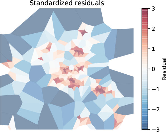
Figure 3: A Voronoi residual map of the self-exciting point process shown in Fig. 2. The model was fit assuming a constant background intensity and does not account for the inhomogeneous rate, leading to positive residuals in the center area and negative residuals outside. Residual values are standardized according to an approximate distribution given by Bray et al. (2014).

4 Applications

This section will review four major applications of self-exciting point processes: earthquake models, crime forecasting, epidemic infection forecasting, and events on networks. This is by no means an exhaustive list—self-exciting point process models have been applied to problems as disparate as wildfire occurrence (Peng, Schoenberg and Woods, 2005) and civilian deaths in Iraq (Lewis et al., 2011). The selected applications illustrate the features that make self-exciting point processes valuable: parameters of the triggering function $g$ have important physical interpretations and can be used to test scientific hypotheses about the event triggering process, while the background $\mu$ flexibly incorporates spatial and temporal covariates whose effects can be estimated. Purely descriptive methods, or methods such as log-Gaussian Cox processes, do not permit the same inference about the event triggering process.

4.1 Earthquake Aftershock Sequence Models

After a large earthquake, a sequence of smaller aftershocks is typically observed in the days and weeks afterwards, usually near the epicenter of the main shock (Freed, 2005). These tremors are triggered by the seismic disturbance of the main shock, and the distribution of their magnitudes and arrival times has proven to be relatively consistent, allowing the development of models for their prediction and analysis.

Sequences of earthquakes and aftershocks show rich behavior, such as spatial and temporal clustering, complex spatial dependence, and gradual shifts in overall seismicity. Self-exciting point processes are a natural choice to model this behavior, as they can directly capture spatio-temporal aftershock triggering behavior and can incorporate temporal trends and spatial inhomogeneity. The Epidemic-Type Aftershock Sequence (ETAS) model, developed and expanded over several decades, provides a flexible foundation for modeling this behavior, and has been widely applied to earthquake sequences in Japan, California, and elsewhere. A comprehensive review is provided by Ogata (1999).

The initial ETAS model was purely temporal, modeling the rate of earthquakes at time $t$ as a superposition of a constant rate of background seismicity and of aftershocks triggered by these background events:

$$\lambda(t)=\mu+\sum_{i\mathrel{\mathop{\mathchar 58\relax}}t_{i}<t}\frac{K_{i}}{(t-t_{i}+c)^{p}}$$

Here $\mu$ is the background seismic activity rate and $K_{i}$ is related to the recorded magnitude $M_{i}$ of earthquake $i$ by the relationship

$$K_{i}=K_{0}e^{\alpha(M_{i}-M_{0})},$$

where $M_{0}$ is the minimum magnitude threshold for earthquakes to be recorded in the dataset, and $K_{0}$, $\alpha$, and $p$ are constants. Earthquake magnitudes are treated as unpredictable marks. The functional form of the triggering function, known as the modified Omori formula, was determined empirically by studies of aftershock sequences.

The temporal ETAS model was soon extended to a spatio-temporal model of the form in eq. (2). A variety of triggering functions $g$ were used, ranging from bivariate normal kernels to more complicated exponential decay functions and power laws; some triggering functions allow the range of spatial influence to depend on the earthquake magnitude. The inhomogeneous background $\mu(s)$, which represents spatial differences in fault structure and tectonic plate physics, can be obtained by a simple kernel density estimate (Musmeci and Vere-Jones, 1992) or by the stochastic declustering methods discussed in Section 3.2.

Zhuang, Ogata and Vere-Jones (2004) demonstrated that stochastic declustering can be used to test model assumptions. They applied the ETAS model and stochastic declustering to a catalog of 19,139 earthquakes compiled by the Japanese Meteorological Agency, then used the declustered data to test assumptions typically used in modeling earthquakes; for example, the distribution of earthquake magnitudes is assumed to be the same for main shocks and aftershocks, and both mainshocks and aftershocks trigger further aftershocks with the same spatial and temporal distribution. By identifying main shocks and aftershocks and connecting them with their offspring, it was possible to test each assumption, finding that some do not hold and leading to a revised model (Ogata and Zhuang, 2006).

Further, by using AIC, different triggering functions have been compared to improve understanding of the underlying triggering mechanisms. For example, spatial power law triggering functions were found more effective than normal kernels, suggesting aftershocks can be triggered at long ranges, and the rate of aftershock triggering depends on the magnitude of the mainshock. This has led to improved earthquake forecasting algorithms based on the ETAS model (Zhuang, 2011). Harte (2012) explored the effects of model misspecification and boundary effects on model fits, finding that a good fit for the background component is also essential, as a poor background fit tends to bias the model to consider background events as triggered events instead, overestimating the rate of triggering and the expected number of offspring events $m$.

Some research suggests that the parameters of the ETAS model are not spatially homogeneous, and that a more realistic model would allow the parameters to vary in space. Ogata, Katsura and Tanemura (2003) introduced a method which allows parameters to vary in space, linearly interpolated between values defined at the corners of a Delaunay triangulation of the space defined by the earthquake locations. To ensure spatial smoothness in these values, a smoothness penalty term was added to the log-likelihood. Nandan et al. (2017) took a similar approach, partitioning the region $X$ drawing $q$ points uniformly at random within $X$, obtaining the Voronoi tesselation, and allowing each Voronoi cell to have a separate set of parameters. No spatial smoothness was imposed, and the number of points $q$ was selected via BIC.

Similar concerns apply to temporal nonstationarity. Kumazawa and Ogata (2014) considered two approaches to model changes in parameters over time: a change-point model, in which parameters are fitted separately to events before and after a suspected change point, and a continuously varying model in which several parameters, including the triggering rate, were assumed to be first-order spline functions in time. Temporal smoothness was enforced with a penalty term in the log-likelihood, and AIC was used to compare the fits in series of earthquakes recorded in Japan, finding evidence of nonstationarity in an earthquake swarm.

4.2 Crime Forecasting

After the development of ETAS models, Mohler et al. (2011) drew an analogy between aftershock models and crime. Criminologists have demonstrated that near-repeat victimization is common for certain types of crime—for example, burglars often return to steal from the same area repeatedly (Short et al., 2009; Townsley, Homel and Chaseling, 2003; Bernasco, Johnson and Ruiter, 2015), and some shootings may cause retaliatory shootings soon after (Ratcliffe and Rengert, 2008; Loeffler and Flaxman, 2017), typically within just a few hundred meters. These can be treated as “aftershocks” of the original crime.

Similarly, several criminological theories suggest the background rate of crime can be expected to widely vary by place. Routine activities theory (Cohen and Felson, 1979) states that criminal acts require three factors to occur together: likely offenders, suitable targets, and the absence of capable guardians. These factors vary widely in space depending on socioeconomic factors, business and residential development, and the activities of police or other guardians (e.g. vigilant neighbors). Rational choice theory (Clarke and Cornish, 1985) considers criminals making rational decisions to commit offenses based on the risks and rewards they perceive—and the availability of low-risk high-reward crime varies in space. Weisburd (2015), using crime data across several cities, argued for a law of crime concentration, stating that a large percentage of crime occurs within just a few percent of street segments (lengths of road between two intersections) in a given city. Bolstering this, Gorr and Lee (2015) demonstrated that a policing program based on both chronic hot spots and temporary flare-ups can be more effective than a program based on only one or the other.

These theories suggest a model of crime which assumes the conditional intensity of crime occurrence can be divided into a chronic background portion, which may vary in space depending on a variety of factors, and a self-exciting portion which accounts for near-repeats and retaliations (Mohler et al., 2011):

$$\lambda(s,t)=\nu(t)\mu(s)+\sum_{i\mathrel{\mathop{\mathchar 58\relax}}t_{i}<t}g(s-s_{i},t-t_{i}),$$

where $g$ is a triggering function and $\nu(t)$ reflects temporal changes from weather, seasonality, and so on. Initially, $\nu$, $\mu$, and $g$ were determined nonparametrically following Algorithm 1, though weighted kernel density estimation was too expensive to perform on the full dataset of 5,376 residential burglaries, so they modified the algorithm to subsample the dataset on each iteration. An alternate approach, requiring no subsampling, would be to use a fast approximate kernel density algorithm to reduce the computational cost (Gray and Moore, 2003).

Mohler (2014) introduced a parametric approach intended to simplify model fitting and also incorporate “leading indicators”—other crimes or events which may be predictive of the crime of interest. In a model forecasting serious violent crime, for example, minor offenses like disorderly conduct and public drunkenness have proven useful in predictions, since they may reflect behavior which will escalate into more serious crime (Cohen, Gorr and Olligschlaeger, 2007). The intensity is simplified to make the background constant in time ($\nu(t)=1$), and to incorporate leading indicators, the background is based on a weighted Gaussian kernel density estimate, in which $\nu(t)=1$ and

$$\mu(s)=\sum_{i=1}^{n}\frac{\alpha_{M_{i}}}{2\pi\eta^{2}T}\exp\left(-\frac{\|s-s_{i}\|^{2}}{2\eta^{2}}\right),$$

where $T$ is the length of the time window encompassed by the dataset, $s_{i}$ and $t_{i}$ the location and time of crime $i$, $M_{i}$ is a mark giving the type of crime $i$ (where $M_{i}=1$ by convention for the crime being predicted), and $\alpha$ is a vector of weights determining the contribution of each event type to the background crime rate. The sum is over all crimes, avoiding the additional computational cost of stochastic declustering. The marks are treated as unpredictable, and only the ground process is estimated, not the conditional distribution of marks.

Similarly to $\mu(s)$, the triggering function $g$ is a Gaussian in space with an exponential decay in time:

$$g(s,t,M)=\frac{\theta_{M}}{2\pi\omega\sigma^{2}}\exp(-t/\omega)\exp\left(-\frac{\|s\|^{2}}{2\sigma^{2}}\right).$$

$\theta$ performs a similar function to $\alpha$, weighting the contribution of each type of crime to the conditional intensity. The bandwidth parameters $\sigma^{2}$ and $\eta^{2}$ determine the spatial influence of a given crime type, while $\omega$ determines how quickly its effect decays in time. In principle, different spatial and temporal decays could be allowed for each type of crime, but this would dramatically increase the number of parameters.

Mohler (2014) fit the parameters of this model on a dataset of 78,852 violent crimes occurring in Chicago, Illinois between 2007 and 2012. The crime of interest was homicide, using robberies, assaults, weapons violations, batteries, and sexual assaults as leading indicators. The resulting model was used to identify “hotspots”: small spatial regions with unusually high rates of crime. Previous research has suggested that directing police patrols to hotspots can produce measurable crime reductions, with results varying by the type of policing intervention employed (Braga, Papachristos and Hureau, 2014). To test the self-exciting model’s effectiveness in this role, Mohler (2014) compared its daily predictions to true historical records of crime, finding that it outperforms methods that consider only fixed hotspots (equivalent to setting $\theta_{i}=0$ for all $i$) and those that only consider near-repeats ($\alpha_{i}=0$ for all $i$).

4.3 Epidemic Forecasting

Forecasting of epidemics of disease, such as influenza, typically rely on time series data of infections or infection indicators (such as physician reports of influenza-like illness, without laboratory confirmation), and hence often rely on time series modeling or compartment models, such as the susceptible–infectious–recovered model (Nsoesie et al., 2013). This data does not typically include the location and time of individual infections, instead containing only aggregate rates over a large area.

When individual-level data is available, however, point processes can model the clustered nature of infections. Spatial point processes have been widely used for this purpose (Diggle, 2014, chapter 9), and when extended to spatio-temporal analysis, self-exciting point processes are a natural choice, with excitation representing the transmission of disease. Again following the ETAS literature, Meyer, Elias and Höhle (2012) introduced a self-exciting spatio-temporal point process model adapted for predicting the incidence of invasive meningococcal disease (IMD), a form of meningitis caused by the bacterium Neisseria meningitidis, which can be transmitted between infected humans and sometimes forms epidemics. Unaffected carriers can retain the bacterium in their nasopharynx, suggesting that observed cases of IMD can be divided into “background” infections, transmitted from an unobserved carrier to a susceptible individual, and triggered infections transmitted from this individual to others.

In a dataset of 636 infections observed in Germany from 2002–2008, each infection’s time, location (by postal code), and finetype (strain) was recorded. The model includes unique features: rather than empirically estimating the background function, it is composed of a function of population density and of a vector of covariates (in this case, the number of influenza cases in each district of Germany, hypothesized to be linked to IMD). The resulting conditional intensity function is

$$\begin{split}\lambda(s,t)={}&\rho(s,t)\exp\left(\beta^{\prime}z(s,t)\right)\\ &{}+\sum_{j\in I^{*}(s,t)}e^{\eta_{j}}g(t-t_{j})f(\|s-s_{j}\|),\end{split}$$

where $I^{*}(s,t)$ is the set of all previous infections within a known fixed distance $\delta$ and time $\epsilon$. Here $\rho(s,t)$ represents the population density, $z(s,t)$ the vector of spatio-temporal covariates, and $\eta_{j}=\gamma_{0}+\gamma^{\prime}m_{j}$, where $m_{j}$ is a vector of unpredictable marks on each event, such as the specific strain of infection. The spatial triggering function $f$ is a Gaussian kernel, and the temporal triggering function $g$ is assumed to be a constant function, as there were comparatively few direct transmissions of IMD in the dataset from which to estimate a more flexible function.

The results were promising, showing that the self-exciting model can be used to estimate the epidemic behavior of IMD. The unpredictable marks $m_{j}$ included patient age and the finetype (strain) of bacterium responsible. Comparisons between finetypes revealed which has the greatest epidemic potential, and the age coefficient allowed comparisons of the spread behavior between age groups.

Meyer and Held (2014) then proposed to replace $f$ with a power law function, previously found to better model the long tails in the movement of people (Brockmann, Hufnagel and Geisel, 2006). Using the asymptotic covariance estimator given in eq. (14), they also produced confidence intervals for their model parameters, though without verifying the necessary regularity assumptions on the conditional intensity function (Meyer, 2010, section 4.2.3). A similar modeling approach was used to test if psychiatric hospital admissions have an epidemic component, via a permutation test for the parameters of the epidemic component of the model (Meyer et al., 2016).

Schoenberg, Hoffman and Harrigan (2017) introduced a recursive self-exciting epidemic model in which the expected number of offspring $m$ of an event is not constant but varies as a function of the conditional intensity, intended to account for the natural behavior of epidemics: when little of the population has been exposed to the disease, the rate of infection can be high, but as the disease becomes more prevalent, more people have already been exposed and active prevention measures slow its spread. The model takes the form

$$\lambda(s,t)=\mu+\int_{X}\int_{0}^{t}H\left(\lambda(s^{\prime},t^{\prime})\right)g(s-s^{\prime},t-t^{\prime})\operatorname{d\!}N(s^{\prime},t^{\prime}),$$

where $g$ is a chosen triggering function and $H$ is the productivity function, determining the rate of infection stimulated by each event as a function of its conditional intensity. Schoenberg, Hoffman and Harrigan (2017) took $H(x)=\kappa x^{-\alpha}$, with $\kappa>0$, to model decreasing productivity, and fit to a dataset of measles cases in Los Angeles, California with maximum likelihood to demonstrate the effectiveness of the model.

4.4 Events on Social Networks

The models discussed so far have considered events in two-dimensional space (e.g. latitude and longitude coordinates of a crime or infection). Recently, however, self-exciting point processes have been extended to other types of events, including events taking place on social networks.

Fox et al. (2016) considered a network of officers at the West Point Military Academy. Each officer is a node on the network, and directed edges between officers represent the volume of email sent between them. Fox et al. (2016) developed several models, the most general of which models the rate at which officer $i$ sends email as

$$\lambda_{i}(t)=\nu_{i}\mu(t)+\sum_{j}\sum_{r_{k}^{ij}<t}\theta_{ij}\omega_{i}e^{-\omega_{i}(t-r_{k}^{ij})}.$$

Here $r_{k}^{ij}$ represents the time of the $k$th message sent from officer $j$ to officer $i$, $\omega_{i}$ is a temporal decay effect for officer $i$, and $\theta_{ij}$ models a pairwise reply rate for officer $i$’s replies to officer $j$. The background rate $\mu(t)$ is allowed to vary in time to model time-of-day and weekly effects, with a offset $\nu_{i}$ for each officer. The model is fit by expectation maximization and standard errors found by parametric bootstrap.

Zipkin et al. (2015) considered the same dataset, but instead of modeling a self-exciting process for each officer, they assigned one to each edge between officers, which enabled them to develop methods for a missing-data problem: can the sender or recipient be inferred if one or both are missing from a given message? The self-exciting model had promising results, and they suggested a possible application in inferring participants in gang violence.

Taking an alternate approach, Green, Horel and Papachristos (2017) modeled the contagion of gun violence through social networks in Chicago. The network nodes were all individuals who had been arrested by Chicago police during the study period, connected by edges for each pair of individuals who had been arrested together, assumed to indicate strong pre-existing social ties. Rather than predicting the rate on edges, as Fox et al. (2016) did, this study modeled the probability of each individual being a victim of a shooting as a function of seasonal variations (the background) and social contagion of violence, as the probability of being involved in a shooting is assumed to increase if someone nearby in the social network was recently involved as well.

This is formalized in the conditional intensity for individual $k$,

$$\lambda_{k}(t)=\mu(t)+\sum_{t_{i}<t}\phi_{k_{i},k}(t-t_{i}),$$

where $\mu(t)$ represents seasonal variation and the self-excitation function $\phi_{k_{i},k}$ is composed of two pieces, a temporal decay $f_{\beta}(t)$ and a network distance $g_{\alpha}(u,v)$:

$$f_{\beta}(t) =\beta e^{-\beta t}$$

$$g_{\alpha}(u,v) =\begin{cases}\alpha\,\text{dist}(u,v)^{-2}&\text{when }\text{dist}(u,v)\leq 3\\ 0&\text{otherwise}\end{cases}$$

$$\phi_{u,v}(t) =f_{\beta}(t)g_{\alpha}(u,v),$$

where $\text{dist}(u,v)$ is the minimum distance (number of edges) between nodes $u$ and $v$. The model was fit numerically via maximum likelihood, and a form of declustering performed by attributing each occurrence of violence to the larger of the background $\mu(t)$ or the sum of contagion from previous events, rather than using a stochastic declustering method as discussed in Section 3.2.

5 Conclusions

When a spatio-temporal point process can be divided into clusters of events triggered by common causes, self-exciting models are a powerful tool to understand the dynamics of the process. This review has highlighted developments in several areas of application which enable fast maximum likelihood and Bayesian estimation, declustering of events, and a variety of model diagnostics. Not all of these tools are widely adopted, particularly graphical diagnostics which have only been developed over the past few years, and there are many open problems: Bayesian estimation, for example, could lead to hierarchical models which consider several separate realizations of a process (such as crime data from different cities), and the application of self-exciting models to data on networks is in its infancy, and likely has many other possible applications.

Interpretation of self-exciting models does require care, however. For example, consider an infectious disease with no known carriers—all transmission is from infected to susceptible individuals, and any given case could, in principle, be traced back to the index case. The division into background and cluster processes makes less conceptual sense here, since there is not a background process producing new cases from nowhere; if a self-exciting model were fit to infection data, the background process would capture cases caused by unobserved infections, and an improved rate of case reporting would decrease the apparent importance of the background process. Unobserved infections would also mean that $m$, the estimated number of infections triggered by each case, would be underestimated, as some triggered infections would not appear in the data.

But when the underlying generative process is clustered, self-exciting spatio-temporal point processes are fast, flexible, and interpretable tools, with growing application in many scientific fields.