Numerical Simulations of Supernova Remnant Evolution in a Cloudy Interstellar Medium

Abstract

The mixed morphology class of supernova remnants has centrally peaked X-ray emission along with a shell-like morphology in radio emission. White & Long proposed that these remnants are evolving in a cloudy medium wherein the clouds are evaporated via thermal conduction once being overrun by the expanding shock. Their analytical model made detailed predictions regarding temperature, density and emission profiles as well as shock evolution. We present numerical hydrodynamical models in 2D and 3D including thermal conduction, testing the White & Long model and presenting results for the evolution and emission from remnants evolving in a cloudy medium. We find that, while certain general results of the White & Long model hold, such as the way the remnants expand and the flattening of the X-ray surface brightness distribution, in detail there are substantial differences. In particular we find that the X-ray luminosity is dominated by emission from shocked cloud gas early on, leading to a bright peak which then declines and flattens as evaporation becomes more important. In addition, the effects of thermal conduction on the intercloud gas, which is not included in the White & Long model, are important and lead to further flattening of the X-ray brightness profile as well as lower X-ray emission temperatures.

1 Introduction

Supernovae are the primary source of hot gas in galaxies. The shocks created in a supernova explosion can expand to distances of more than 100 pc and create large, hot, low density volumes of gas that persist for millions of years. Supernova remnant (SNR) evolution has been explored theoretically for several decades with increasing levels of complexity. However, the appearance of SNRs and the way the shocks couple with the interstellar medium (ISM) depend crucially on the nature of the medium into which the remnant expands, in particular its density and inhomogeneity.

For many years SNRs were divided into two categories, shell-like and plerionic. The first category has emission that peaks at the edge of the remnant while plerions are centrally brightened. It was believed that in the latter case a pulsar wind powers the emission, while for shell-like remnants, emission from the outer blastwave shock dominates. However, cases that did not fit either morphology were found and referred to as either thermal composite, because of their centrally concentrated and yet thermal X-ray emission along with edge brightened radio emission, or mixed morphology supernova remnants (MMSNR).

Rho & Petre (1998) first argued that the mixed morphology remnants formed a truly distinct class of SNRs. In more recent years more remnants in this class have been found and evidence has been presented that these remnants are, as a rule, undergoing interactions with dense clouds. In particular Yusef-Zadeh et al. (2003) showed a strong correlation of OH maser emission with mixed morphology, indicating that shocks in molecular clouds are present around MMSNRs. In addition, shock-cloud interaction indicators such as broad velocity wings (Frail & Mitchell, 1998) or an enhanced ${}^{12}\mathrm{CO}(J=2-1)/^{12}\mathrm{CO}(J=1-0)$ ratio (Seta et al., 1998) are observed in many MMSNRs (see review by Slane et al., 2015).

At present, there are $\sim 40$ known MMSNRs, but the nature of the central X-ray emission is poorly understood. X-ray spectra show evidence for the presence of ejecta in some such MMSNRs, but the inferred mass of the X-ray emitting material appears to be much larger than any reasonable ejecta contributions. The observed temperature profiles show little variation with radius, in contrast to the steep profile associated with the Sedov phase. Possibly related is the observation that the plasma in many MMSNRs is observed to be overionized (e.g., Kawasaki et al., 2002; Yamaguchi et al., 2009), indicating a rapid cooling phase (Uchida et al., 2012; Moriya, 2012).

Nearly half of the known MMSNRs are observed to produce gamma-ray emission, presumably indicating the interaction between protons accelerated by the SNR (or re-accelerated cosmic rays) and molecular cloud material or dense post-shock regions of radiative shocks (Uchiyama et al., 2010; Lee et al., 2015).

Even well before many of these observations that characterized MMSNRs in detail, White & Long (1991, hereafter WL) put forward an analytical model that attempted to explain remnants with centrally peaked X-ray emission. WL included terms in the fluid equations describing evolution in spherical symmetry of a SNR that allowed for a continual injection of mass and momentum as the result of cloud evaporation. In this way they aimed to describe the evolution and emission distribution generated when a SN explodes in a cloudy medium and where thermal conduction evaporates the clouds that have been enveloped by the blastwave. We note that there was no term in the equations accounting for the transfer of energy within the hot gas by thermal conduction. We will discuss the ramifications of this further below.

2 Methods

WL created their models for SNR evolution in a cloudy medium starting from the usual set of equations for hydrodynamics under the assumption of spherical symmetry but with added terms to account for the effects of cloud evaporation on the mass, momentum and energy in the remnant. Though they included a term for mass injection into the intercloud medium as a result of thermal conduction, as mentioned above, they did not explicitly include thermal conduction. For our numerical hydrodynamical calculations presented here we employ the code FLASH (Fryxell et al., 2000, 2010, http://flash.uchicago.edu/site/flashcode/) without any extra terms added to account for mass loss from clouds since they are unnecessary in multiple dimensions as long as the physics is correctly modeled. An essential aspect of the modeling is the inclusion of thermal conduction, which is accurately and efficiently included via the Diffuse module included in version 4.3 of FLASH. We discuss the details of our use of this module in the appendix. The initial conditions for our cloudy medium runs include an initial distribution of clouds in space with varying sizes. The cloud size distribution and density were not important for WL as long as the fundamental assumptions of their calculations were not violated, namely that the clouds are much denser than the intercloud medium, the clouds are uniformly distributed in space and the filling factor of the clouds is small. We fulfill these criteria by randomly placing clouds that are a factor of 100 times denser than the intercloud medium with an overall small volume filling factor (dictated by the $C$ parameter, see below). We set off the SN explosion in this medium by putting the appropriate amount of thermal energy in a small number of parcels at the center of the remnant. We do not include any ejecta mass, which would be important at early times during the ejecta dominated phase. The characteristic time for the transition from the ejecta dominated to Sedov phase is (Truelove & McKee, 1999) $t_{ch}=E^{-1/2}M_{\mathrm{ej}}\rho^{-1/3}$, which for our values of explosion energy and density, and assuming 5 $M_{\odot}$ of ejecta, is about 2700 yr. It will take several times this value for the evolution to truly settle into a Sedov solution evolution in the remnant as a whole, though the approach will be faster for the region behind the forward shock. For this reason we do not expect the early time evolution (e.g. X-ray luminosity) to be very realistic (though of course this also applies to the WL model). In our runs the thermal energy leads to rapid expansion and partial conversion of the thermal energy to kinetic energy as expected for Sedov-Taylor expansion (e.g., Chevalier, 1974). Most of the results we discuss in this paper were carried out in 2D cylindrical symmetry, though we have done runs in 3D as well as a check on the effects of the 2D assumption.

For all of our runs, we use an explosion energy of $10^{51}$ ergs. As with the Sedov-Taylor solution, we expect the explosion energy to set the overall scale of the remnant but not to affect such things as the division of energy between thermal and kinetic forms. We use an ambient intercloud density of 0.25 cm^-3 and a temperature of $10^{4}$ K. These values are typical for the warm interstellar medium, though the temperature is perhaps slightly high for realistic heating and cooling balance. The exact value for the temperature should not have a significant affect on our results. The clouds are assumed to have a density of 25 cm^-3, which then leads to a temperature of 100 K to maintain pressure balance in the ambient medium. (Note that we are not tracking the ionization which would change these values if the ionization level were lower in the clouds than in the intercloud medium.) These values are consistent with typical cold neutral (H I) cloud values. We do not expect the cloud temperature to be important to the remnant evolution. The cloud density could have some effect, since a larger density, for the same ratio of cloud mass to intercloud mass, would imply a lower cloud filling factor, though we think that our assumed density is realistic. For the cloud sizes we use a power law in radius. We took the distribution used in McKee & Ostriker (1977), which was partly based on observations by Hobbs (1974) and has lower and upper radius cutoffs of 0.48 and 10 pc and a power law exponent of -3 in radius. We create realizations of the cloud distribution by drawing randomly from this power law distribution and also choosing cloud location randomly within the simulation volume. We discard clouds that overlap with previously generated clouds such that each cloud is distinct from all the others. We also discard clouds that extend outside of the simulation volume. For our 2D cylindrically symmetric runs the clouds are, in effect, tori with circular cross sections. In our 3D runs, which are done in cartesian coordinates, the clouds are true spheres.

The actual cloud size distribution in the Galaxy is poorly constrained and so our adopted parameters of the cloud size distribution may not accurately reflect the true cloud size distribution, (though others have found similar results, e.g. Gosachinskij & Morozova, 1999; Chieze & Lazareff, 1980). There is evidence that interstellar clouds have a morphology that is closer to filamentary or “clumpy sheets” (Heiles & Troland, 2003), though more regular clouds are observed as well. We do not expect the cloud geometry to have a very substantial effect on SNR evolution or observables since, once shocked, the complex flows inside the remnant create large distortions of the clouds in any case. However, if a remnant encounters a cloud that is comparable in size to the remnant, both the appearance and evolution of the remnant would be strongly affected. In such cases the remnant would have a strongly asymmetric appearance. Exploration of such cases is beyond the scope of this paper.

WL found that their solutions could be parametrized by just two parameters: $C$, the ratio of the mass in clouds to that in the intercloud medium, and $\tau$ the ratio of the cloud evaporation timescale to the remnant age. While $C$ is clearly a fixed value that characterizes the conditions in the ambient medium, WL concede that $\tau$ may not be. Since the temperature of the interior of a remnant evolves with time and the evaporation timescale would generally be expected to depend on the temperature and/or the pressure. In fact it can be shown, using the results of Dalton & Balbus (1993), that in the limit of highly saturated evaporation, the evaporation timescale is $\tau_{\mathrm{evap}}\propto R_{\mathrm{cl}}^{7/6}P^{-5/6}$, with no explicit dependence on temperature. Since the pressure in the Sedov-Taylor solution drops as $t^{-6/5}$, if the medium surrounding the enveloped clouds is close to that for Sedov-Taylor expansion in a uniform medium, we expect that the evaporation timescale should be proportional to the remnant age and so $\tau$ should be constant. Deviations from these assumptions, for example because the evaporation is not highly saturated or because the cloud-cloud or cloud-shock interactions cause substantial deviations from a Sedov-Taylor evolution that lead to different evolution of the evaporation rate, would then be expected to cause variation of $\tau$ with remnant age. We discuss this further below.

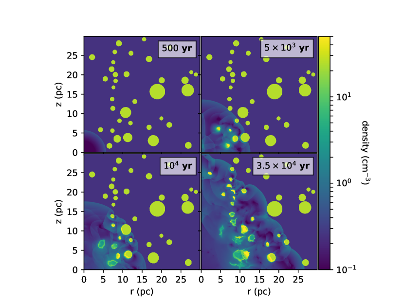
Figure 1: Snapshots of the density for a 2D cylindrically symmetric run of SNR evolution in a cloudy medium. The cloud filling factor is set by the WL parameter $C=10$.

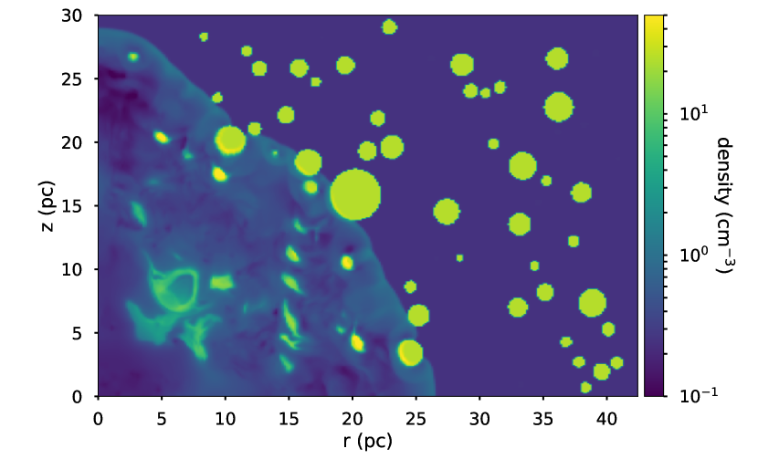
Figure 2: Slice of the density for a 3D run of SNR evolution in a cloudy medium, again with WL parameter $C=10$. The slice is taken parallel to the $z$ axis and at a 45$\arcdeg$ angle to the $x$ and $y$ axes. The age of the remnant here is $3.5\times 10^{4}$ yr.

3 Results

In Figure 1 we show the density for four snapshots of the evolution for one simulation. For this case we use a value for the WL parameter $C=10$, ratio of mass in clouds to that in the intercloud medium. Given the definition of $C$, the volume filling factor of clouds is

$$f=\frac{C}{\chi+C}$$ (1)

where $\chi$ is the ratio of the cloud density to the intercloud density. With our assumption that $\chi=100$, for the $C=10$ case, $f=0.091$. For our 2D cylindrically symmetric runs, the clouds are really toroids. However, for these cases the area filling factor, that is the fraction of the $r-z$ plane filled with clouds, is quite close to the volume filling factor of the toroidal clouds. If the clouds are evenly distributed in cylindrical radial distance this will always be the case. We have explored a range of $C$ values ranging from 3 to 30. We take 10 as our standard case for much of the discussion in this paper. Figure 2 shows the density for a slice through one of our 3D runs. That run also had $C=10$. Note the similar area filling factor for the clouds. The fact that it is a slice through a 3D volume results in the cloud radii appearing systematically smaller than the true cloud radii.

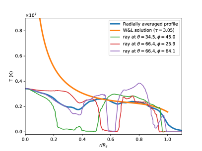
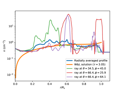
Figure 3: Temperature (left) and density (right) radial profiles for a 3D run. The rays show all the variations along the particular sight line as indicated in the legend (using spherical coordinate) while the “radially averaged” curves only include the parcels that are hot ($T>10^{5}$ K). The “W&L solution” curves show the WL type profiles for the actual values of $C$ in the simulation and the value for $\tau$ that results in the same mass in hot gas as in the simulation. The SNR age for this run is $2.5\times 10^{4}$ yr.

In Figure 3 we show temperature and density profiles for the same 3D run as in Figure 2. The rays shown illustrate the variations along a line of sight from the origin outward along the direction given by the angles listed in the legend. We also show the radially averaged profiles for temperature and density, but for those we exclude cloud material, here defined as parcels with temperature below $10^{5}$ K. The averaging is done by calculating a volume weighted sum of all parcels within each radial bin that have hot gas in them and dividing by the volume of parcels (whether or not they have hot gas) in the same radial bin. The WL profile uses the actual value of $C$ for the simulation at the given time ($2.5\times 10^{4}$ yr) and given the current shape of the shock front ($C=9.0$), which is calculated as the mass in clouds within the shock front divided by the mass in the intercloud medium inside the same volume, both for the initial, undisturbed medium. The value of $\tau$ used is that which leads to the same mass of hot gas as for the simulation. We see that, while for much of the outer parts of the remnant, the radially averaged profile is similar to the WL profile, in the inner region the density and temperature stay flat for the simulation while the WL profile has a steeply rising temperature and falling density similar to a Sedov-Taylor type profile. In addition, the density variations, as well as averaged values, are important for the X-ray emission, as discussed below, since emissivity goes as density squared.

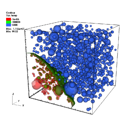
Figure 4: 3D rendering of the shock and clouds for one of our 3D runs. The cloud and shock surfaces are shown as temperature contours. The age of the remnant is $1.5\times 10^{4}$ yr. The box is 30 pc on a side. Note the strong distortions of the shock front.

3.1 Shock Evolution

The similarity solution of WL results in expansion of the shock front with the same power law in time as for the Sedov-Taylor solution, i.e. $R_{s}\propto t^{2/5}$. For our calculations, evaluating the shock radius is not entirely straightforward since in regions where a cloud is being encountered the shock is slowed and the front in general is complex. In Figure 4 we show 3D contours of the shock and clouds which illustrate the complexity of the shock front. We found that the simplest approach and the one that is closest to what one would find from observations is to find the outermost pressure contour that is substantially above the ambient pressure, $P/k_{B}=10^{4}$ cm^-3 K for our case with an ambient pressure of 5200 cm^-3 K, and use that to calculate the volume inside the remnant. The shock radius is then just $R_{s,\mathrm{eff}}=(3V_{s}/4\pi)^{1/3}$, where $V_{s}$ is the volume enclosed by the shock. (Note: the find_contours and grid_points_in_poly methods in the scikit-image measure python module provide effective methods for finding parcels inside the shock.) This leads to a relatively smooth shock expansion except for some cases in which the shock wraps around a large cloud leading to a jump in the shock radius. An alternative and easier approach is to use the volume of hot gas to define the shock radius, though in that case the volume in the clouds contained in the SNR is not included. In practice for our calculations that volume is small compared with the hot gas volume and the derived shock radius is very similar.

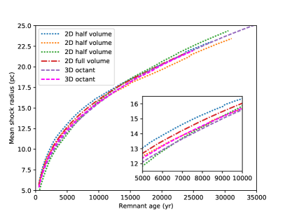
Figure 5: Evolution of the mean shock radius for different $C=10$ runs. This illustrates the variations that are possible with different cloud realizations. We note that the shock evolutions for the 3D cases are consistent with the 2D cylindrically symmetric cases as is the 2D case using the full volume (positive and negative $z$). The inset shows a detail to illustrate more clearly the differences during a medium age period.

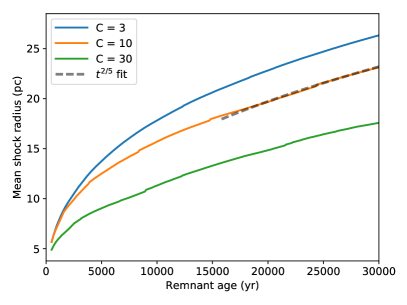
Figure 6: Comparison of the evolution of the mean shock radius for runs with different values for $C$, the ratio of ISM mass in clouds to that in the intercloud medium. The density of the clouds and the intercloud medium is the same for all of the runs, $25$ cm^-3 and $0.25$ cm^-3, respectively. Only the filling factor of the clouds is varied. As expected larger $C$ values lead to slower shock expansion. The dashed curve labeled “$t^{2/5}$ fit” is a fit to the shock radius evolution assuming that $R_{s}\propto t^{2/5}$ for the $C=10$ case, where the fitting was done only for the range in $t$ as plotted. This shows that the evolution approaches the $t^{2/5}$ law found by WL. For this case an effective density, i.e. the density that the corresponding Sedov-Taylor expansion would require, is 0.455 cm^-3.

For our calculations we do find that the shock evolution depends to some degree on the particular cloud realization used. This is illustrated in Figure 5 which shows the shock evolution for several different cloud realizations. For most of our runs we have used only half of the 2D volume, $z\geq 0$. The figure shows that the shock evolution for different runs using the 2D half volume differ though the variations are at about the 10% level. We have tested the effects of using the 2D half volume by doing a full volume run, shown as the red dash-dotted line in Figure 5. We find no significant difference in that run as compared with other runs with the same $C$ value. We have also compared with a 3D runs (using one octant of the space) done in cartesian coordinates. Again, as demonstrated in Figure 5 we find no significant difference from the 2D half volume runs. Because of the computational and visualization demands of the 3D runs, they were done with only 5 levels of grid refinement rather than the 6 levels used for the 2D runs. We have found, by doing 2D runs at 5 and 6 levels of refinement, that while there are minor differences in the density distributions, with more filamentary structure visible in the higher resolution runs, the overall evolution of the remnants are nearly identical. Thermal conduction aids in this respect since small scale details tend to be smoothed out when it is included.

The expansion law for the runs shown in Figure 5 is generally not far from the WL $t^{2/5}$ value, though again there are significant variations around that. One way to test that is to compute $v_{s}t/r_{s}$, which for a $t^{2/5}$ expansion law should give 2/5. Doing this involves taking numerical derivatives of the shock radius expansion curve which inevitably results in a noisy curve. In general we find that the expansion law is close to but slightly below this value on average, though with excursions above and below it.

In Figure 6 we show the shock radius evolution for runs with different $C$ values. Since the mean density in the medium increases with $C$ it is expected that the shock expansion rate should decrease as $C$ increases. In the results of WL, the expansion rate is characterized via the parameter $K$ (their equation 8) where

$$r_{s}=\left[\frac{25(\gamma+1)KE}{16\pi\rho_{1}}\right]^{1/5}t^{2/5},$$ (2)

$r_{s}$ is the shock radius, $E$ is the explosion energy, $\gamma=5/3$, and $\rho_{1}$ is the ambient intercloud density (0.25 cm^-3 for our runs). WL lists values for $K/K(\mathrm{Sedov})$ as a function of $\tau$, the ratio of cloud evaporation time to remnant age. $K(\mathrm{Sedov})=1.528$ is the $K$ value for the case of no clouds. We can invert equation 2 to determine the effective value of K for our runs. Doing this we find that K varies considerably over a typical run though it flattens at late times. For most of our runs, K defined this way starts high, $>2$, but ends near 0.9. The WL model predicts, given a value of $\tau$ of $\sim 5-10$ (see discussion below) and $C=10$, $K\sim 0.816-1.149$. This is in fairly good agreement with our results. K can also be alternatively be defined using WL’s equation (6) as

$$K=\frac{4\pi\rho_{1}r_{s}^{3}v_{s}^{2}}{(\gamma+1)E}.$$ (3)

With this definition, we find more stable values for K, which still fall roughly in the predicted range.

3.2 Cloud Evaporation Rate

Within the WL model the value of $\tau$, the ratio of evaporation timescale to remnant age, is treated as a free parameter. In our numerical work, this is not the case, since given the initial conditions the cloud evaporation timescale will follow from the physics, including the temperature of the surrounding hot gas and the complex heat flow patterns that develop as the clouds are both evaporated and disrupted by shear flows. In addition, clouds close to the explosion center can be heated enough by being shocked that they could be considered part of the hot gas, though still overdense. However, as we discuss below, such clouds are overpressured compared to the surrounding medium and so they expand and cool at later times in the remnant evolution.

Clouds that are farther from the center do not get heated to high temperatures by the expanding shock but are subject to shear flows and thermal conduction. However, even for these clouds, characterizing the evaporation rate is not entirely straightforward since gas exists at a range of temperatures and densities within the remnant at any given time. As a result defining which gas has been evaporated is not entirely clear cut.

We have tried a variety of approaches for determining the effective evaporation timescale for our simulated remnants. One approach is to use a density criterion to decide what is cloud material and what is evaporated. In our case we defined the mass in clouds as the mass of gas with density above a 2.5 cm^-3, which is the geometric mean of the density of intercloud medium, 0.25 cm^-3, and the cloud density, 25 cm^-3. The mass of gas evaporated from clouds at any given point in the remnant’s evolution is then the mass that was in clouds initially within the shock volume minus the mass in clouds at the current time. The average evaporation rate is then the evaporated mass divided by the remnant age. Connecting this evaporation rate to that predicted in the WL model is not entirely straightforward however, since they did not tally that quantity. Instead we can connect the intercloud mass, that is all the mass inside the shock that is not in a cloud, with the total integrated mass in the WL model since the density, $\rho$, or scaled density, $g=\rho/\rho_{s}$ stands for all the non-cloud gas in the model. Thus we compare the intercloud gas in a simulation with

$$M_{x}=\int_{0}^{r_{s}}4\pi r^{2}\rho\,dr=4\pi r_{s}^{3}\rho_{s}\int_{0}^{1}g(x)x^{2}\,dx,$$ (4)

(from WL) where $g\equiv\rho/\rho_{s}$ is derived by integrating the set of equations in WL for given values of $\tau$ and $C$. To find the value of $\tau$ corresponding to a particular time for a simulated remnant we use the actual value for $C$, calculated as the initial ratio of mass in clouds to that in the intercloud medium within the shock volume. We then do a search, using a root finding method, wherein we calculate the values of $M_{x}$ given values of $\tau$ until we match the value for the simulated remnant. This is the method used to produce Figure 7.

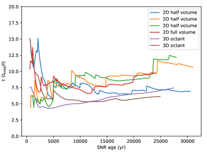
Figure 7: Evaporation timescale factor, $\tau$, of WL vs. remnant age. In the WL model $\tau$ is a constant, but here we see that it varies considerably over the age of our simulated remnants. The 3D runs show smoother behavior because more clouds are sampled at any given age. Here $\tau$ is calculated using the density criterion for deciding whether gas is intercloud or cloud gas with $n<2.5$ cm^-3 as the dividing line. All the runs plotted here have $C$ set to 10.

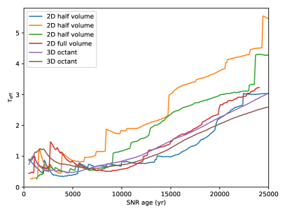
Figure 8: Evaporation timescale factor, $\tau$, of WL vs. remnant age. In this case we use the temperature criterion to differentiate between cloud and intercloud gas with $T>10^{5}$ K as the dividing line. This method ensures that the X-ray emitting gas mass (though not the luminosity) for the corresponding WL model matches that for the simulated remnant. The $\tau$ values calculated this way are substantially below those in Figure 7, primarily because of hot, but still dense, gas generated by shocking clouds close to the explosion center. Such gas is counted as cloud gas (and thus not evaporated) by the method of the previous figure, but should radiate X-rays.

Another approach is to calculate the mass of X-ray emitting gas, essentially all gas in the remnant that is hotter than 10⁵ K, and match that with the X-ray emitting mass, $M_{x}$, for a given WL model. That approach leads to values of $\tau$ that are considerably lower than for the density based criterion, mostly because of the production of hot, dense gas via shock heating. The results for $\tau$ using the temperature based criterion are shown in Figure 8.

The status of the shocked cloud gas is somewhat ambiguous in the model, however since it is overpressured when shocked and some of it re-expands and cools adiabatically at later times below X-ray emitting temperatures. For clouds shocked by slower shocks, only a surface layer is raised to X-ray emitting temperatures. Thus, at later times, the removal of material from clouds is primarily by thermal conduction and cloud evaporation as discussed by WL does apply.

We expect that the evaporation timescale for the remnant as a whole should depend in a similar way to that for individual clouds (though see Balbus, 1985, regarding the effect on evaporation rate of a collection of clouds). For “classical” evaporation, i.e. cloud evaporation when the heat flux is far from saturation, the evaporation timescale goes as $t_{\mathrm{evap}}\propto R_{\mathrm{cl}}^{2}n_{\mathrm{cl}}T_{h}^{-5/2}$ where $R_{\mathrm{cl}}$ is the cloud radius, $n_{\mathrm{cl}}$ is the cloud density and $T_{h}$ is the temperature of the hot gas far from the cloud. In the case of highly saturated heat flux, which is the more typical condition in SNRs during the non-radiative phase, we get $t_{\mathrm{evap}}\propto R_{\mathrm{cl}}^{7/6}n_{\mathrm{cl}}P^{-5/6}$, where $P$ is the thermal pressure in the hot gas. Since, ignoring the effects of shocks, the density in the clouds is expected to be roughly constant and, as mentioned above, the pressure should decrease as $t^{-6/5}$, the evaporation timescale should increase proportional to $t$. From this we would expect the WL parameter $\tau\equiv t_{\mathrm{evap}}/t$ to be roughly constant and to only depend on the density and size of the clouds.

For our assumptions regarding mean mass per particle we find

$$t_{\mathrm{class}}=3.02\times 10^{14}\frac{R_{\mathrm{cl}}^{2}n_{\mathrm{cl}}}{T_{h}^{5/2}}\;\mathrm{Myr}$$ (5)

and

$$t_{\mathrm{sat}}=1.48\times 10^{3}\frac{R_{\mathrm{cl}}^{7/6}n_{\mathrm{cl}}}{P_{h}^{5/6}}\;\mathrm{Myr}$$ (6)

where $R_{\mathrm{cl}}$ is the cloud radius in pc, $n_{\mathrm{cl}}$ is the cloud density in cm^-3, $T_{h}$ is the temperature of the surrounding hot gas and $P_{h}$ is the thermal pressure (presumed to be roughly equal in the cloud and hot gas) in cm^-3 K. We find that with these values, it is not typical to get values for $\tau$ less than one. These expressions also make it clear that the primary determinant of the $\tau$ value is the cloud size distribution. We have confirmed this by doing runs with smaller clouds, using 0.2 and 5.0 pc as the lower and upper size limits, but with the same volume filling factor (and thus $C$ value). As expected we find that the clouds evaporate faster, leading to smaller values of $\tau$.

While our discussion above indicates that $\tau$ should be roughly constant, we find that it evolves considerably over the course of SNR evolution. This is not too surprising since, especially for the 2D evolution, a small number of clouds is encountered and the location and size of the clouds affects the evaporation rate. This is demonstrated in Figures 7 and 8 where we plot $\tau$, calculated two different ways, as a function of remnant age for a variety of our runs. The differences between the 2D runs can be attributed to the differences in the particular cloud realization for the runs with some with larger clouds placed closer to the origin and the spacing of clouds differing. As can be seen, the 3D runs show less variation between themselves and over time. This can be understood as deriving from the larger number of clouds encountered and thus more complete sampling of the cloud size distribution. A full volume 3D run would likely show an even smoother variation though the finite cloud volume would still be expected to create variations over the course of the cloud evolution. There is some indication here that there is faster evaporation (smaller $\tau$) in the 3D simulations than in the 2D simulations, which could be understood as being caused by the larger surface area to volume ratio effectively for the spherical clouds in 3D than for the toroids under cylindrical symmetry. Nevertheless, the shock expansion does not show any marked difference between 2D and 3D cases nor does the calculated X-ray emission as we discuss in the next section.

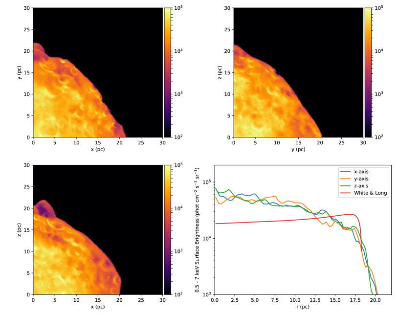
Figure 9: Brightness profiles for a 3D run in the $0.5-7$ keV band. The images are created by integrating along a given axis while the lower right line plot is radially averaged in addition. The emissivity assumes collisional ionization equilibrium and uses APEC (Foster et al., 2012; Smith et al., 2001) to calculate the photon emissivity as a function of temperature. The age of the remnant is $1.5\times 10^{4}$ yr. For the White & Long curve we used the actual values determined at the given time for the values for $C$ and $\tau$ which are 7 and 9 respectively.

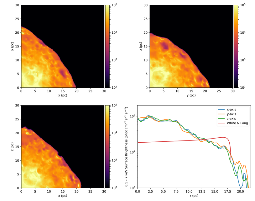
Figure 10: Same as Figure 9 except for a run with a different cloud realization. The differences in the brightness profiles illustrate the level of variation caused by differences in the random distribution of clouds in the ambient medium.

3.3 X-ray Emission Distribution

One of the principal motivations for the WL model was to explain the appearance of SNRs with centrally peaked thermal X-ray emission. WL showed that they could achieve a range of different X-ray emission distributions depending on the choice of their parameters $C$ and $\tau$. From their Figure 4 it can be seen that centrally peaked X-ray emission requires values of $C\gtrsim 20$, depending on the value of $\tau$. For $\tau=2$ (WL Figure 4a) none of the emission profiles is truly centrally peaked. With $\tau=10$ (WL Fig. 4b) centrally peaked emission is achieved, though only for fairly high $C$. For our evaluation of the emission in our simulated remnants we have chosen to use a more realistic emissivity than the constant $\Lambda_{x}=10^{-22}$ ergs cm³ s^-1 used by WL (note that in the units for this coefficient, the exponent for cm in WL was mistakenly shown as -3 rather than 3). Here we use a photon emissivity for optically thin emission in the $0.5-7$ keV band (see Figure 11) as calculated using APEC (Foster et al., 2012; Smith et al., 2001) with the assumption of collisional ionization equilibrium (CIE). We discuss the assumption of CIE below.

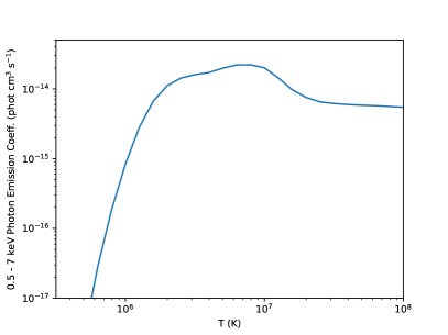
Figure 11: Emission coefficient for optically thin radiative cooling by gas in collisional ionization equilibrium. This coefficient is for photons emitted in the $0.5-7$ keV band and includes both line and continuum emission.

This choice of emission coefficient covers a typical X-ray observation energy range, e.g. with Chandra. From Figure 11 it is clear that this emissivity weights the emission profile strongly toward gas in the temperature range of $\sim 10^{6.5}-10^{7}$. A detector with sensitivity at lower energies could see the emission from lower temperature gas generated at the boundaries of the clouds which is expected to be strong. The lower right panels of Figures 9 and 10 show a comparison of the WL profile that corresponds with the $\tau$ and $C$ values at that time for each run. Note that here we use the effective value for $C$ rather than the mean value. By this we mean that we use $C=m_{\mathrm{cl}}/m_{\mathrm{ic}}$ where $m_{\mathrm{cl}}$ is the cloud mass, $m_{\mathrm{ic}}$ is the intercloud mass and both are for the initial medium contained within the current volume of the shock. This will tend to make the effective $C$ smaller than the mean value over the whole medium because the shock is slowed where it encounters clouds, though in practice we have found this effect to be fairly minor. The same APEC emissivity was used to generate the WL profile as for those from the simulations. The relative flatness of the WL profile is caused by the lower density and higher temperature near the center as compared with the simulations (see Figure 3).

Figure 12: Evolution of the $0.5-7$ keV photon luminosity in our simulations. At early times the luminosity is low because the very high gas temperature and because few clouds have been encountered. The peak in emission comes when the shock encounters clouds and is still fast enough that the shock transmitted into the clouds can heat gas to X-ray emitting temperatures. Later cloud evaporation raises the hot gas density while expansion lowers the pressure, leading to roughly constant luminosity.

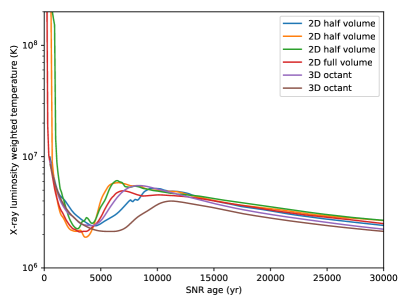
Figure 13: Evolution of the X-ray weighted temperature in simulated remnants. At the time of peak luminosity, much of the emission is coming from relatively low temperature shocked cloud gas, which leads to low temperature emission. At later times more of the emission comes from the hot intercloud gas which is hotter.

The evolution of the $0.5-7$ keV photon luminosity is shown in Figure 12 for several simulations with $C=10$. The emissivity-weighted temperature is shown in Figure 13. The luminosity starts low both because the remnant volume is low (i.e. the shock radius is small) and because the temperature is very high, above the temperature range of highest emission efficiency in the band (see Figure 11). (Note that because we do not include ejecta mass or extra circumstellar material, the very early emission is not expected to be accurately modeled.) The luminosity then reaches a peak at an age of $\sim 2000$ yr. This peak is associated with a time when the SNR encounters its first cloud. The shock is fast enough at this point (in our runs) to heat the entire cloud to X-ray emitting temperatures. Later the clouds close to the explosion site re-expand and cool (adiabatically since we have not included radiative cooling). This is because the shocked clouds are overpressured relative to the intercloud medium and also the pressure in the remnant is decreasing as it expands. An example of this can be seen in Figure 2 where a hollow looking cloud can be seen which has re-expanded and cooled. These clouds cool enough that they fall below X-ray emitting temperatures, i.e. $T\lesssim 10^{5}$ K. For clouds farther from the origin, only their inward facing edges get heated sufficiently to produce X-rays (see the arcs in Figure 9). Cloud material at those later times is continually being evaporated off the clouds, which increases the density of the hot gas, but at the same time the expansion of the remnant cools the gas. The net result, as can be seen from the figure, is an almost flat or slightly decreasing X-ray photon luminosity. This contrasts with the behavior predicted by WL (their eq. 21) which is for the luminosity to increase in proportion to the remnant volume. The evolution of the emissivity weighted temperature of the emission has a nearly inverted profile compared with the luminosity evolution. That can be explained by the fact that the shocked cloud gas is relatively cool, though dense, so when that gas is hot enough to emit X-rays, the emissivity-weighted temperature is low. As a remnant transitions to the phase where most of the emission is coming from the lower density and hotter gas, the emission temperature increases and then flattens out.

These differences in luminosity evolution are some of the most substantial differences between our calculated results and the WL model. The domination of the emission by the shocked cloud gas shows that the MM remnant’s brightness distribution, especially at early times, does not depend as much on evaporated mass as on the shock interactions of the blast wave with the clouds. In this sense, the value of $\tau$ derived based on density, as shown in Figure 7 is not such an important parameter, though it is consistent with our expectations for the evaporation timescale, including the fact that it is roughly constant during remnant evolution. Instead the effective $\tau$, shown in Figure 8, where the temperature of the gas is the criterion for differentiating cloud gas from intercloud gas is a better measure for understanding the X-ray luminosity evolution, though given that some of that gas later cools via expansion, this $\tau$ is not a good measure of gas that has been thermally evaporated.

4 Discussion

There are a number of additional processes that could affect SNR-cloud interaction in the ISM. Chief among these is radiative cooling. WL did not include cooling and we do not include it in our results presented here, though we intend to explore it in future work. In preliminary calculations we have found that the shape and size of shocked clouds is strongly affected, but the overall evolution of the remnant, for ages early enough that the remnant has not yet gone radiative as a whole, is not substantially changed. Korolev et al. (2015) have recently studied the longer term evolution of SNR evolution in a cloudy medium including radiative cooling but not thermal conduction with 2D numerical simulations.

If radiative cooling is important, then non-equilibrium ionization should be taken into account. In SNRs in general and for shocks into clouds in particular, we expect the post shock gas to be underionized and far from CIE. This is also true for gas that is evaporated from the entrained clouds (Ballet et al., 1986; Slavin, 1989). It is also expected that the hot gas that was created early in the remnant’s lifetime will be overionized after the remnant has expanded and cooled. This effect will be enhanced by the presence of thermal conduction which draws thermal energy away from the hot interior toward the cooler outer parts of the remnant. In addition there could be turbulent mixing in the medium that would combine hot and cold gas producing yet another type of non-equilibrium ionization state (Slavin et al., 1993). All of these effects can have potentially large impacts on the emitted X-ray spectrum if the ionization is sufficiently far from CIE. These effects will need to be taken into account in order to make quantitative predictions for the emission spectrum for SNRs evolving in a cloudy ISM. We are currently in the process of improving the treatment of non-equilibrium ionization by FLASH, which will then allow efficient and accurate calculations of NEI effects.

Another possibly important influence on remnant evolution is the magnetic field. The field can affect the overall expansion of the remnant as well as the evaporation of clouds in the remnant. The anisotropic thermal conduction within the remnant when the clouds are threaded by the field is likely to have complex effects which deserve to be studied in detail. Our aim in the current study has been to examine SNR evolution under conditions similar to those intended in WL and so we do not include the magnetic field at this stage. Finally, we do not include heating via photoionization. This could be important in the post-shock regions of radiative shocks but is likely a minor effect for the young to middle-aged remnants evolving in the low density, warm ISM such as we examine in this work.

5 Conclusions

The WL model was put forward in an attempt to explain the mixed morphology class of SNRs as being caused by the evaporation of dense clouds that are overrun by the blast wave. We have presented numerical hydrodynamical models of SNRs evolving in a cloudy medium including thermal conduction in order to test whether the results of WL hold up when more of the physics is included. We find that some of their results are broadly confirmed including: remnants expand with roughly the same $t^{2/5}$ power law dependence on age as a standard Sedov-Taylor expansion, 2) the cloud evaporation timescale increases roughly in proportion to the remnant age (i.e. $\tau$ is roughly constant), and 3) the presence of clouds causes the remnant X-ray brightness to be centrally peaked. However, the lack of the inclusion of the dynamical effects of cloud-shock interaction and thermal conduction within the hot gas that are present in multidimensional calculations lead to substantial differences from the results of WL. Probably the largest difference is with the predicted X-ray luminosity evolution which, rather than rising in proportion to the shocked volume, has an early peak and then flattens to a nearly constant level. This can be traced to the shock heating of the clouds close to the explosion site, which provides the peak, and later to the expansion cooling of the shocked clouds along with a transition to evaporative mass loss as the dominant mass loss mechanism for the clouds. The differences in temperature and density distribution in the remnants caused by thermal conduction within the hot gas and the shocking of the clouds leads to a flat X-ray brightness distribution in the remnants. For certain combinations of parameters, the brightness profile for WL models can match that from our models, though the parameters do not correspond to the physics, i.e. evaporation timescale and cloud-to-intercloud mass ratio, actually present in the simulation. In general we find that the X-ray emission weighted temperature is lower for our models than for WL models because of the inclusion of lower temperature hot gas associated with the clouds, either shocked or evaporated gas.

Our results point to important differences from the WL model for SNRs evolving in a cloudy ISM which could have implications for the interpretation of SNR observations, particularly in the X-rays. However, to make more robust predictions, particularly for the X-ray spectrum, will require the inclusion of more physical processes in future simulations. In particular radiative cooling and non-equilibrium ionization could substantially affect the observed spectrum of SNRs such as those we have modeled. We have begun to look at the effects of these processes and those calculations will allow us to make detailed predictions for the spectra of mixed morphology SNRs in future work.

Appendix A FLASH parameters for the use of thermal conduction

The Diffuse module of FLASH uses a number of parameters that govern how thermal conduction is calculated. Both standard Spitzer conductivity, $\kappa\propto T^{5/2}$, and saturated conductivity (McKee & Cowie, 1977) $\kappa\propto\rho c^{3}$ are supported with a smooth transition from “classical” to saturated governed by the saturation parameter $\sigma$. The parameter values that we have used in the flash.par files for runs with thermal conduction included are listed in table 1. The particular unit that we used is included via the switch -unit=physics/Diffuse/DiffuseMain/Unsplit to the setup command. In addition, to use the power law conductivity, we added REQUIRES physics/materialProperties/Conductivity/ ConductivityMain/PowerLaw to the Config file in our simulations directory. With these settings, electron thermal conduction is used with a power law conductivity, $\kappa=aT^{5/2}$ modified by the saturation limit from Cowie & McKee (1977) and using the harmonic mean weighting (chosen through the diff_eleFlMode parameter) as in Balbus & McKee (1982), $q=(1/q_{\mathrm{class}}+1/q_{\mathrm{sat}})^{-1}$, where $q_{\mathrm{class}}$ is the “classical” Spitzer heat conduction and $q_{\mathrm{sat}}$ is the “saturated” conduction, which corresponds to the heat flux being transported at the maximum rate possible by the electrons, $q_{\mathrm{sat}}=5\phi_{s}\rho c^{3}$. Balbus & McKee (1982) argue that $\phi_{s}\approx 0.3$ (though with substantial uncertainty) and we use that value in this work. Here $a$ is the Spitzer conductivity coefficient (Spitzer, 1962), $1.84\times 10^{-5}/ln\Lambda$, where $\Lambda$ is the Coulomb logarithm. For conditions that we are exploring, $a\approx 6\times 10^{-7}$. In FLASH the implementation of saturation uses $q_{\mathrm{sat}}=\alpha_{\mathrm{ele}}\rho_{\mathrm{ele}}c_{\mathrm{ele}}^{3}$ effectively, so to use $\phi_{s}=0.3$ we set $\alpha_{\mathrm{ele}}=0.04491$. This is derived under the assumption of a fully ionized plasma with a He abundance of 10% by number. These assumptions also lead to setting eos_singleSpeciesA to 0.6123. In reality the cooler parts of the plasma will most likely be partially ionized or nearly neutral, though in those regions conductivity is very low in any case. The parameter diff_thetaImplct sets the scheme for the diffusion solver, where 0.5 is for the Crank-Nicholson method, 0.0 for fully explicit and 1.0 for fully implicit. As indicated in the table, we use the Crank-Nicholson scheme. Since that scheme is unconditionally stable we set the dt_diff_factor to $10^{10}$ so as to effectively prevent the very restrictive diffusion timestep constraint from limiting the timestep.

We have tested the thermal conductivity by calculating the steady evaporation of a spherical cloud in cylindrical symmetry (in 2D) under moderately saturated conditions. The resulting mass loss rate and temperature profile closely matched that predicted by the results of Dalton & Balbus (1993) who found analytical solutions for steadily evaporating clouds as a function of the degree of saturation. These results give us confidence that thermal conduction is functioning correctly in the code.

Table 1: Diffusion related parameters settings for FLASH runs with conductivity

parameter name	parameter value
useConductivity	.true.
useDiffuse	.true.
useDiffuseTherm	.true.
dt_diff_factor	1.E10
cond_densityExponent	0.0
cond_temperatureExponent	2.5
cond_K0	6.E-7
diff_useEleCond	.true.
diff_eleFlMode	fl_harmonic
diff_eleFlCoef	0.04491
diff_thetaImplct	0.5
diff_eleXlBoundaryType	zero-gradient
diff_eleXrBoundaryType	zero-gradient
diff_eleYlBoundaryType	zero-gradient
diff_eleYrBoundaryType	zero-gradient
diff_eleZlBoundaryType	zero-gradient
diff_eleZrBoundaryType	zero-gradient

References

- Balbus (1985) Balbus, S. A. 1985, ApJ, 291, 518
- Balbus & McKee (1982) Balbus, S. A., & McKee, C. F. 1982, ApJ, 252, 529
- Ballet et al. (1986) Ballet, J., Arnaud, M., & Rothenflug, R. 1986, A&A, 161, 12
- Chevalier (1974) Chevalier, R. A. 1974, ApJ, 188, 501
- Chieze & Lazareff (1980) Chieze, J. P., & Lazareff, B. 1980, A&A, 91, 290
- Cowie & McKee (1977) Cowie, L. L., & McKee, C. F. 1977, ApJ, 211, 135
- Dalton & Balbus (1993) Dalton, W. W., & Balbus, S. A. 1993, ApJ, 404, 625
- Foster et al. (2012) Foster, A. R., Ji, L., Smith, R. K., & Brickhouse, N. S. 2012, ApJ, 756, 128
- Frail & Mitchell (1998) Frail, D. A., & Mitchell, G. F. 1998, ApJ, 508, 690
- Fryxell et al. (2000) Fryxell, B., Olson, K., Ricker, P., et al. 2000, ApJS, 131, 273
- Fryxell et al. (2010) —. 2010, FLASH: Adaptive Mesh Hydrodynamics Code for Modeling Astrophysical Thermonuclear Flashes, Astrophysics Source Code Library, , , ascl:1010.082
- Gosachinskij & Morozova (1999) Gosachinskij, I. V., & Morozova, V. V. 1999, Odessa Astronomical Publications, 12, 113
- Heiles & Troland (2003) Heiles, C., & Troland, T. H. 2003, ApJ, 586, 1067
- Hobbs (1974) Hobbs, L. M. 1974, ApJ, 191, 395
- Kawasaki et al. (2002) Kawasaki, M. T., Ozaki, M., Nagase, F., et al. 2002, ApJ, 572, 897
- Korolev et al. (2015) Korolev, V. V., Vasiliev, E. O., Kovalenko, I. G., & Shchekinov, Y. A. 2015, Astronomy Reports, 59, 690
- Lee et al. (2015) Lee, S.-H., Patnaude, D. J., Raymond, J. C., et al. 2015, ApJ, 806, 71
- McKee & Cowie (1977) McKee, C. F., & Cowie, L. L. 1977, The Astrophysical Journal, 215, 213
- McKee & Ostriker (1977) McKee, C. F., & Ostriker, J. P. 1977, ApJ, 218, 148
- Moriya (2012) Moriya, T. J. 2012, ApJ, 750, L13
- Rho & Petre (1998) Rho, J., & Petre, R. 1998, ApJ, 503, L167
- Seta et al. (1998) Seta, M., Hasegawa, T., Dame, T. M., et al. 1998, ApJ, 505, 286
- Slane et al. (2015) Slane, P., Bykov, A., Ellison, D. C., Dubner, G., & Castro, D. 2015, Space Sci. Rev., 188, 187
- Slavin (1989) Slavin, J. D. 1989, ApJ, 346, 718
- Slavin et al. (1993) Slavin, J. D., Shull, J. M., & Begelman, M. C. 1993, ApJ, 407, 83
- Smith et al. (2001) Smith, R. K., Brickhouse, N. S., Liedahl, D. A., & Raymond, J. C. 2001, ApJ, 556, L91
- Spitzer (1962) Spitzer, L. 1962, Physics of Fully Ionized Gases (Interscience Publishers)
- Truelove & McKee (1999) Truelove, J. K., & McKee, C. F. 1999, ApJS, 120, 299
- Uchida et al. (2012) Uchida, H., Koyama, K., Yamaguchi, H., et al. 2012, PASJ, 64, 141
- Uchiyama et al. (2010) Uchiyama, Y., Blandford, R. D., Funk, S., Tajima, H., & Tanaka, T. 2010, ApJ, 723, L122
- White & Long (1991) White, R. L., & Long, K. S. 1991, ApJ, 373, 543
- Yamaguchi et al. (2009) Yamaguchi, H., Ozawa, M., Koyama, K., et al. 2009, ApJ, 705, L6
- Yusef-Zadeh et al. (2003) Yusef-Zadeh, F., Wardle, M., Rho, J., & Sakano, M. 2003, ApJ, 585, 319