The Effect of Atmospheric Cooling on the Vertical Velocity Dispersion and Density Distribution of Brown Dwarfs

Abstract

We present a Monte Carlo simulation designed to predict the vertical velocity dispersion of brown dwarfs in the Milky Way. We show that since these stars are constantly cooling, the velocity dispersion has a noticeable trend with spectral type. With realistic assumptions for the initial-mass function, star-formation history, and the cooling models, we show that the velocity dispersion is roughly consistent with what is observed for M dwarfs, decreases to cooler spectral types, and increases again for the coolest types in our study ($\sim$T9). We predict a minimum in the velocity dispersions for L/T transition objects, however the detailed properties of the minimum predominately depend on the star-formation history. Since this trend is due to brown dwarf cooling, we expect the velocity dispersion as a function of spectral type should deviate from constancy around the hydrogen-burning limit. We convert from velocity dispersion to vertical scale height using standard disk models, and present similar trends in disk thickness as a function of spectral type. We suggest that future, wide-field photometric and/or spectroscopic missions may collect sizable samples of distant ($\sim\!1$ kpc) of dwarfs that span the hydrogen-burning limit. As such, we speculate that such observations may provide a unique way of constraining the average spectral type of hydrogen-burning.

1 Introduction

Brown dwarfs are substellar objects that lack the necessary mass to sustain hydrogen fusion in their cores (e.g. Kumar, 1962; Hayashi & Nakano, 1963). Hence, these objects are constantly cooling throughout their lifetimes (e.g. Burrows, Hubbard, & Lunine, 1989), which leads to the known mass-age degeneracy: a brown dwarf detected with a specific temperature could have a range of ages, depending on its mass (e.g. Baraffe & Chabrier, 1996; Burrows et al., 1997).

Disk kinematics are powerful probes of the structure and evolution of the Milky Way, but also provide constraints on the process of star formation. It is commonly accepted that stars are formed in giant molecular clouds that occupy a thin Galactic disk, then diffuse over time by successive interactions with the disk material (e.g. Spitzer & Schwarzschild, 1951). This so-called disk heating can be used as a Galactic chronometer, which makes stellar kinematics a weak tracer of stellar population age (e.g. Wielen, 1977). Nearby populations of early-M dwarfs are observed to have kinematic ages of $\sim\!3$ Gyr (e.g. Reid et al., 2002; Reiners & Basri, 2009), but extending this chronology to the substellar population is not trivial, particularly if their formation process differs from that of main-sequence stars. Luhman (2012) review the proposed formation scenarios for brown dwarfs and the various effects on their initial kinematics and present-day spatial distributions. Early formation models speculated that brown dwarfs are preferentially ejected from their birthsites (e.g. Reipurth & Clarke, 2001), which should enhance their initial velocities and imply kinematic ages older than the main-sequence population. Most kinematic and spatial distributions of cluster brown dwarfs seem to rule out the ejection scenario, and favor models that have initial kinematics comparable to main-sequence stars (e.g. White & Basri, 2003; Joergens, 2006; Luhman et al., 2006; Parker et al., 2011). Moreover disk brown dwarfs are reported with a range of kinematic ages, in same cases younger than M-dwarfs (e.g. Zapatero Osorio et al., 2007; Faherty et al., 2009; Schmidt et al., 2010) or older (e.g. Seifahrt et al., 2009; Blake, Charbonneau, & White, 2010; Burgasser et al., 2015). Whether the lack of empirical consensus stems from some observational effect (such as small sample size) or points to new astrophysics (such as formation mechanisms) is not readily clear. However brown dwarf kinematics provide important insights into their formation, cooling, and disk heating.

The effect of atmospheric cooling on populations of brown dwarfs has been discussed in great detail throughout the literature, but there are three works that are particularly relevant to our study. (1) Burgasser (2004) present a series of Monte Carlo simulations to predict the present-day mass function (PDMF) of brown dwarfs. Using various assumptions for the initial mass function (IMF), birth rate, and cooling models (Burrows et al., 1997; Baraffe et al., 2003), they confirm the relatively low number density of mid-L dwarfs, even for shallow IMFs. (2) Deacon & Hambly (2006) develop a similar calculation to model the present-day luminosity function (PDLF), which have been used to rule out extreme (halo-type) birth rates (Day-Jones et al., 2013) and confirm the low space density of L/T transition dwarfs (Marocco et al., 2015). The increasing number of late-T field dwarfs has been seen in several studies (e.g. Metchev et al., 2008; Kirkpatrick et al., 2012; Burningham et al., 2013), which is seemingly a pile up of cool dwarfs. (3) Burgasser et al. (2015) propose a two-phase star-formation history to explain the old kinematic ages ($6.5\pm 0.4$ Gyr) of L dwarfs in their sample of 85 M8–L6 dwarfs. Therefore the aim of our work is to build on such kinematic models and predict the vertical number density of brown dwarfs in the Galactic disk.

We organize this paper as follows: in Section 2 we describe our Monte Carlo simulation, in Section 3 we present our estimates for the disk thickness, in Section 4 we discuss our results in the context of what can be achieved with the next generation of surveys, and in Section 5 we summarize our key findings.

2 Monte Carlo Simulations

To characterize the effects of brown dwarf cooling on their Galactic properties, we develop a simple Monte Carlo simulation that is similar to several other studies (e.g. Reid et al., 1999; Burgasser, 2004; Day-Jones et al., 2013; Burgasser et al., 2015). We start with the usual assumption that the creation function is separable in mass and time:

$$C(m,t)\,\mathrm{d}m\,\mathrm{d}t=\phi(m)\,\psi(t)\,\mathrm{d}m\,\mathrm{d}t,$$ (1)

where $\phi(m)$ is the IMF and $\psi(t)$ is the star-formation history (SFH). Although these two distributions are often the focus of many studies, we only wish to adopt plausible functional forms and reasonable range of parameters to set bounds on the effects of atmospheric cooling. Therefore we use a powerlaw IMF

$$\phi(m;\alpha)\,\mathrm{d}m\propto m^{-\alpha}\,\mathrm{d}m,$$ (2)

for $0.0005\!\leq\!m\!\leq\!0.1~{}M_{\odot}$, and we consider models with $\alpha\!\in\![0,0.5,1.0,1.5]$, but discuss the role of these mass limits in Appendix A. For these mass limits, our simulation is valid for spectral types $\sim$M8–T9.

We adopt a gamma-distribution form for the SFH:

$$\psi(t;\beta,\tau)\,\mathrm{d}t\propto\left(\frac{t}{\tau}\right)^{\beta}\exp\left(-\frac{t}{\tau}\right)\,\frac{\mathrm{d}t}{\tau}$$ (3)

for $0\!\leq\!t\!\leq\!t_{0}$, where $t_{0}$ is the age of the Milky Way, which we take to be 12 Gyr. To avoid confusion, we use $t$ to refer to the time since the formation of the Milky Way disk and $a$ as the age of a brown dwarf. These two quantities are related as: $a\!=\!t_{0}-t$. We consider models with $\tau\!\in\![0.3,0.5,0.7,0.9,1.1]~{}\mathrm{Gyr}$ and $\beta\!\in\![2.5,3.5,4.5,5.5,6.5]$ (an exponential model being the special case of $\beta\!=\!0$). The parameters $\beta$ and $\tau$ represent the power-law slope at early times ($t\!\ll\!\tau$) and the exponential decay at late times ($t\!\sim\!\tau$), respectively. This parameterization of the SFH has a maximum star-formation rate at $t_{max}\!=\!\tau\beta$, and it is qualitatively similar to that proposed by Snaith et al. (2015). Also, this SFH is consistent with that of the typical Milky Way-like galaxy (Papovich et al., 2015), which we estimate from their work will have $(\beta,\tau)\!\approx\!(4.5,0.7~{}\mathrm{Gyr})$.

With these two distribution functions, the creation of simulated brown dwarfs is parameterized by three tunable values $(\alpha,\beta,\tau)$, which we refer to as the galaxy model. For each galaxy model, we draw $10^{9}$ random masses and formation times (or ages) from Equations 2 and 3, respectively.

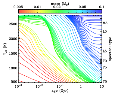
Figure 1: Cooling curves from Burrows et al. (1997). Here we show the effective temperature as a function of age. The lines represent the tracks expected for different stellar masses, as indicated by their color and the color map at the top. The dashed lines indicate the min/max mass for our study. We transform between effective temperature and spectral type using the relation derived by Filippazzo et al. (2015). For our non-cooling models, we hold the temperature and spectral type fixed to the value at 1 Myr.

We adopt the cooling models of Burrows et al. (1997) for solar metallicity to describe the effective temperature as a function of stellar mass and age. In Figure 1, we show these cooling models with appropriate spectral type ranges indicated (see Equation 4 below for additional details). Although we expect metallicity to affect the way brown dwarfs cool, our primary goal is to illustrate the order-of-magnitude effect of cooling and will discuss additional concerns with metallicity-dependent models in Section 4. To determine the current effective temperatures, we linearly interpolate these cooling models for the simulated masses and ages.

To compare our simulations to observations, we must convert between effective temperature ($T_{eff}$) and spectral type (${\cal S}$), and we adopt the polynomial model derived by Filippazzo et al. (2015) for field dwarfs:

$$T_{eff}({\cal S}) = 4747-700.5\times({\cal S}-60)$$ (4)

$$+115.5\times({\cal S}-60)^{2}$$

$$-11.91\times({\cal S}-60)^{3}$$

$$+0.6318\times({\cal S}-60)^{4}$$

$$-0.01606\times({\cal S}-60)^{5}$$

$$+0.0001546\times({\cal S}-60)^{6},$$

where $T_{eff}$ is Kelvin and ${\cal S}$ is the numeric spectral type. Throughout this work, we encode spectral type for dwarf stars as starting at 0 (for O0V), incrementing by 10 for each major spectral type and by 1 for each minor type. For example, a G2V star is represented as ${\cal S}\!=\!42$. The Filippazzo et al. (2015) relation is valid for $66\!\leq\!{\cal S}\!\leq\!89$ (M6–T9). We also considered the Stephens et al. (2009) temperature-type relation and find similar results to those discussed below.

We assign vertical velocities to our simulated stars using the results of Wielen (1977), who solves the Fokker-Planck equation and demonstrates that the vertical velocity dispersion increases with age. Under different assumptions for the velocity and/or time dependence of the diffusion coefficient, Wielen (1977) derives various relationships between the vertical velocity dispersion and the age of the population. We adopt the velocity-dependent diffusion coefficient that varies with time, as it offers the highest degree of flexibility, which gives a velocity dispersion of the form:

$$\sigma_{v}^{3}=\sigma_{v,0}^{3}+\frac{3}{2}\,\gamma_{v,p}\,T_{\gamma}\,\left(\exp\left(\frac{a}{T_{\gamma}}\right)-1\right),$$ (5)

where ($\sigma_{v,0},\gamma_{v,p},T_{\gamma}$) are tunable parameters to be determined from observations. Given the observations of cluster brown dwarfs (e.g. Moraux & Clarke, 2005), we assume that brown dwarf initial kinematics are comparable to main-sequence stars. Therefore we use the vertical velocity dispersions of Dehnen & Binney (1998) and Aumer & Binney (2009) as a calibration set. However, these results are reported as a function of spectral type, not age as we require. Therefore we compute the average stellar population birth time, weighted over the adopted SFH:

$$\left<t({\cal S})\right>=\frac{\int_{t^{\prime}}^{t_{0}}t\,\psi(t)\,\mathrm{d}t}{\int_{t^{\prime}}^{t_{0}}\psi(t)\,\mathrm{d}t}$$ (6)

where the lower limit of integration is $t^{\prime}\!=\!t_{0}-t_{MS}({\cal S})$ and $t_{MS}({\cal S})$ is the main-sequence lifetime as a function of spectral type:

$$\log t_{MS}({\cal S}) = 0.92+0.040\times({\cal S}-40)$$ (7)

$$-0.00051\times({\cal S}-40)^{2}$$

$$+0.000045\times({\cal S}-40)^{3}$$

where $t_{MS}({\cal S})$ is in gigayears — Equation 7 is polynomial fit to tabulted data (Lang, 1993). Now the SFH-weighted average age is: $\left<a({\cal S})\right>\!=\!t_{0}-\left<t({\cal S})\right>$. Since this transformation between spectral type and age depends on the SFH through Equation 6, it must be computed for each combination of $(\beta,\tau)$. In Table 2, we give best-fit values for $(\sigma_{w,0},\gamma_{w,p},T_{\gamma})$ and reduced $\chi^{2}_{\nu}$ determined for stars with $t_{MS}({\cal S})\!\leq\!t_{0}$ (${\cal S}\!\lesssim\!44$). The values originally quoted by Wielen (1977) are for the three-space velocity dispersion, but here we explicitly only deal with $w$-component of the velocity dispersion. In fact, the vertical velocity dispersions quoted by Wielen (1977) in their Table 1 yield similar results to our estimates in Table 2: $\sigma_{w,0}\!=\!9$ km s^-1, $\gamma_{w,p}\!=\!68$ (km s^-1)³ Gyr^-1, and $T_{\gamma}\!=\!2$ Gyr. In Figure 2, we show the kinematic data with the calibrated diffusion law for the SFH of $(\beta,\tau)\!=\!(4.5,0.7~{}\mathrm{Gyr})$.

We have verified that our choice of the parameterization of the diffusion law does not dictate our findings discussed below by considering the alternatives (e.g. Wielen, 1977; Aumer & Binney, 2009). Of course, the parameter values of the diffusion law depend strongly on the diffusion model and the SFH, but the key aspect is that we must capture the trend of increasing velocity dispersion with population age or main-sequence lifetime (see Figures 2 or 3 for examples).

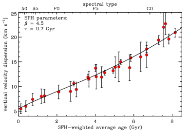
Figure 2: Calibrated diffusion law. The data points here are taken from Dehnen & Binney (1998) and Aumer & Binney (2009), and the solid line represents the best fit to the velocity-dependent diffusion model where the diffusion constant varies with time (Equation 16 of Wielen, 1977). We convert between spectral type and SFH-weighted average age using the assumed SFH (see Equation 6), and therefore this diffusion law must be calibrated for each unique combination of the SFH parameters. Here we show the nominal model of $(\beta,\tau)\!=\!(4.5,0.7~{}\mathrm{Gyr})$, which is consistent with a Milky Way-like galaxy (Papovich et al., 2015).

With the diffusion model calibrated for the choice of SFH, we have a self-consistent description for the velocity dispersion as a function of stellar age. The velocity dispersion measured for a population over a range of spectral types (or effective temperatures) will be:

$$\left<\sigma^{2}_{w}\right>=\frac{1}{N}\sum_{i=1}^{N}\sigma^{2}_{w}(a_{i})$$ (8)

where $N$ is the number of samples in the desired spectral type range. Now the simulated parameter $\left<\sigma^{2}_{w}\right>^{1/2}$ is directly comparable to published estimates for the velocity dispersion.

We also consider a non-cooling model to establish a baseline for comparison. Here we repeat the above procedure, but fix the effective temperature to the value at 1 Myr and increase the velocity dispersion according to the same calibrated Wielen (1977) diffusion laws. At this point we have a library of simulated dwarfs, each of which has been assigned mass, age, effective temperature, spectral type, and vertical velocity, all of which are consistent with our assumptions on the IMF, SFH, cooling models, and calibrated observations (such as Equation 4 or Equation 7). We construct this library for the suite of galaxy models listed above, and compute various distributions to compare with observations.

As a final note, we present the analytic integral in Appendix B that is approximated by this Monte Carlo simulation.

3 Results

Using our libraries of simulated disk brown dwarfs, we are able to compute several quantities, namely, the distribution of spectral types, luminosities (assuming the $M_{J}(\mathrm{Vega})-{\cal S}$ relation described by Dupuy & Liu, 2012), and PDLFs. We confirm the findings presented by Burgasser (2004); Day-Jones et al. (2013); Marocco et al. (2015), but omit their presentation here for brevity. Instead, we turn to develop a unique component stemming from the kinematics of the brown dwarf population.

In Figure 3, we show the expected vertical velocity dispersion as a function of spectral type, where the data points are taken from the literature (see the figure caption for details) and the red/blue lines indicate our cooling/non-cooling models, respectively. All of our galaxy models show a few characteristic behaviors: First, the velocity dispersions from the non-cooling models are always constant, and roughly consistent with what is seen in low-mass dwarfs. Second, the cooling models have a roughly constant velocity dispersion for $\sim$M8–L2, then decrease significantly. The shape, depth, and minimum spectral type of this deviation depend on the adopted galactic model ($\alpha,\beta,\tau$). Our goal here is not to constrain these model parameters and/or attempt to reproduce the brown dwarf kinematic measurements, but rather point out that this deviation occurs for any reasonable choice of the galaxy model. Additionally, the deviation is only present when we allow the brown dwarfs to cool, which suggests that atmospheric cooling may leave an imprint on the Galactic-scale distribution of brown dwarfs at fixed spectral type. Third, the T/Y-transition objects generally have velocity dispersions consistent with the M-dwarfs, suggesting that atmospheric cooling for L-dwarfs proceeds faster than diffusion throughout the disk (e.g. Burgasser, 2004).

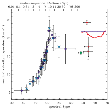
Figure 3: Example vertical velocity dispersion. Here we show our model kinematics for $(\alpha,\beta,\tau)\!=\!(0.5,4.5,0.7~{}\mathrm{Gyr})$ with the cooling (red line) and non-cooling (blue line) models for brown dwarfs. The data points are taken from the literature ((dark-blue circles: Dehnen & Binney, 1998), (light-blue stars: Aumer & Binney, 2009), (right-facing triangles: Reiners & Basri, 2009), and (pentagons: Burgasser et al., 2015)). We indicate spectral types that are above the hydrogen-burning limit as shades of blue, types that plausibly straddle the limit as green, and types likely entirely below the limit as shades of red. The non-cooling models (blue line) are always constant and the cooling models (red line) deviate significantly, generally reaching a minimum between L5–T0. It is important to stress, our intention is not to reproduce the brown dwarf observations, but rather to demonstrate the effects of cooling on their kinematics. We consider this deviation as evidence that the atmospheric cooling may leave a detectable signature in the brown dwarf kinematics.

As mentioned above, the properties of the deviation depend on the choice of galaxy model. We find that the power-law slope of the IMF has the least importance, and our range of IMF slopes can only account for a $\lesssim\!1\%$ change in the depth of the deviation. Furthermore the SFH parameters ($\beta,\tau$) have considerably more effect details of the deviation, which is qualitatively consistent to the Burgasser et al. (2015) finding. To investigate that somewhat further, we consider the ratio of star-formation in the last 2 Gyr to that in the first 2 Gyr of the life of the Milky Way:

$$R=\frac{\int_{10}^{12}\,\psi(t)\,\mathrm{d}t}{\int_{0}^{2}\,\psi(t)\,\mathrm{d}t},$$ (9)

as a means of tracing the fraction of young-to-old brown dwarfs. In Figure 4 we show the maximum deviation in the velocity dispersion (computed as the maximum difference between the non-cooling and cooling models) as a function of the ratio of recent-to-old star-formation; the data points are color coded by the IMF slope. We see that the deviation is largest for SFHs that are dominated by recent star formation, further suggesting that cooling is a key effect. We find that maximum deviation generally occurs for spectral types L5–T0.

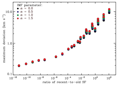
Figure 4: Velocity dispersion deviation. We show the maximum deviations (defined as the maximum difference between the non-cooling and cooling models) as a function of the ratio of recent-to-old star formation (as defined by Equation 9). The color of the plot symbol refers to the power-law slope of the IMF (black: $\alpha\!=\!0$, blue: $\alpha\!=\!0.5$, green: $\alpha\!=\!1$, and red: $\alpha\!=\!1.5$). The SFH has the largest influence on the properties of the velocity dispersion deviation illustrated in Figure 3, with the IMF slope playing a lesser role. The additional assumptions, such as diffusion law and mass limits, are largely irrelevant in dictating the velocity dispersion deviations.

These results are almost completely insensitive to many of our underlying assumptions. First, the range of masses in the IMF has no significant effect on these results provided the mass range is within the range reliably sampled by the cooling models (see Appendix A). Second, the choice of the velocity-dispersion parameterization has little effect, other than to say it is necessary that the velocity dispersion must predict the precipitous increase seen in spectral types $\lesssim$G4V shown in Figure 3.

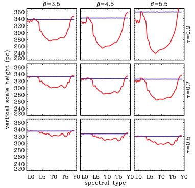
Figure 5: Predicted vertical scale height. We convert from velocity dispersion to scale height assuming the $n\!=\!2$ model developed by van der Kruit (1988) and a disk surface mass density of $\Sigma\!=\!68~{}M_{\odot}~{}\mathrm{pc}^{-2}$ (Bovy & Rix, 2013). As in Figure 3, the non-cooling/cooling models are indicated by solid blue/red lines, respectively. Here we show $\alpha\!=\!0.5$ with a range of ($\beta,\tau$), centered on the baseline value estimated by Papovich et al. (2015). Current modeling techniques have the accuracy to detect a change of $\Delta z_{scl}\!\approx\!50$ pc (e.g. Ryan et al., 2011), however few surveys have the sufficient sample size and spectral type resolution/accuracy needed to resolve such deviations.

As outlined in Section 1, many studies find that the vertical velocity dispersions of L dwarfs is larger than that of M dwarfs (e.g. Seifahrt et al., 2009; Blake, Charbonneau, & White, 2010; Burgasser et al., 2015). To examine this effect, Burgasser et al. (2015) developed a very similar Monte Carlo simulation to our work, and they see hints of the deviation described above for comparable Galactic models. However they propose a two-phase SFH where brown dwarfs are systematically older than main-sequence stars, which they assume are formed at a constant rate throughout the life of the Milky Way. In this way, their two-phase Monte Carlo simulation predicts a roughly increasing or constant velocity dispersion between the late-M and early-L dwarfs. This effect seems to naturally arise in our models (see Figure 3), which is a consequence of our SFH that has more late-time star formation. Moreover, our model predicts the strongest deviation from constancy for types later than $\sim$L4, for which the Burgasser et al. (2015) sample is limited (6/85).

Table 1: Estimates of the Vertical Scale Height^†

Reference	spectral type	$z_{scl}$	Notes
		(pc)
Chen et al. (2001)	F0–M4	$330\pm 3$	type computed from Covey et al. (2007)
Zheng et al. (2001)	$\cdots$	300	spectral type not clear
Ryan et al. (2005)	$>$M6	$350\pm 50$
Pirzkal et al. (2005)	$>$M4	$400\pm 100$
Jurić et al. (2008)	M0–M4	$\sim\!250$	additionally fit thick disk and halo, types computed
			from Covey et al. (2007)
Pirzkal et al. (2009)	M4–M9	$370_{-65}^{+60}$
Pirzkal et al. (2009)	M0–M9	$300\pm 70$
Bochanski et al. (2010)	M0–M8	$300\pm 15$	additionally fit thick disk component
Ryan et al. (2011)	$>$M8	$290\pm 40$
Holwerda et al. (2014)	M5–M9	$400\pm 100$	use $\operatorname{sech}^{2}(\cdot)$ model
van Vledder et al. (2016)	M0–M9	$290\pm 20$	additionally fit halo component

4 Discussion

We have demonstrated that atmospheric cooling may leave an imprint on the kinematics as a function of spectral type via disk heating, since hot brown dwarfs must be young. By somewhat reversing this argument, we can use observations as a function of spectral type to place constraints on the spectral type of the hydrogen-burning limit, averaged over metallicity. Many kinematic surveys do not have sufficient sample sizes to permit examination of velocity dispersions in fine bins of spectral type, as may be needed to see the deviations predicted here. Furthermore, most kinematic samples are limited to the earliest L-dwarfs, and we predict the deviations to begin around $\sim$L3 (c.f. Burgasser et al., 2015). However it may be possible to leverage the known relationships between disk thickness ($z_{scl}$) and velocity dispersion, then use brown dwarf number counts as a similar tool (e.g. Bahcall, 1986). van der Kruit (1988) proposes a flexible family of vertical density distributions that can explain a host of observational phenomena:

$$\rho(z)=2^{-2/n}\rho_{scl}\operatorname{sech}^{2/n}\left(\frac{n\,z}{2\,z_{scl}}\right),$$ (10)

where $n$ is the shape parameter. The classic isothermal disk solution and exponential parameterization are special cases where $n\!=\!1$ and $n\!=\!\infty$, respectively. This class of functions leads to the following relationship:

$$z_{scl}=\zeta_{n}\,\frac{{\sigma_{20}}^{2}}{\Sigma_{68}},$$ (11)

where $\sigma_{20}$ and $\Sigma_{68}$ are the velocity dispersion in units of 20 km s^-1 (the average value of main-sequence stars: $\mathrm{G0}\!\geq\!{\cal S}\!\geq\!\mathrm{M9}$, see Figure 3) and the surface mass density in units of 68 $M_{\odot}~{}\mathrm{pc}^{-2}$ (Bovy & Rix, 2013), respectively. The normalization constant depends on the shape parameter:

$$\zeta_{n}\approx\begin{cases}217~{}\mathrm{pc}&n=1\\ 277~{}\mathrm{pc}&n=2\\ 435~{}\mathrm{pc}&n=\infty.\end{cases}$$ (12)

We convert our predicted velocity dispersion to vertical scale height using the $n\!=\!2$ model (van der Kruit, 1988; de Grijs & van der Kruit, 1996) in Figure 5. Assuming the baseline model of $(\alpha,\beta,\tau)\!=\!(0.5,4.5,0.7~{}\mathrm{Gyr})$, we predict that a pure late-L/early-T dwarf sample should occupy a disk that has a scale height of $z_{scl}\!\sim\!280$ pc, which is about $\sim\!15\%$ thinner than what is seen for late-M dwarfs (see Table 1). Additionally, the critical point in Figure 5 where the cooling-model (red line) scale heights deviate from the non-cooling model (blue line) is $\sim$L3, which would be indicative of an absolute lower-bound on the hydrogen-burning limit for solar metallicity. Through careful calibration of the dwarfs that are known to be burning hydrogen (such as by the lithium test), it may be possible to relate the spectral type of deviation to the hydrogen-burning limit. Since the velocity dispersions of T/Y transition objects is similar to that of the M-dwarfs, we expect Y-dwarfs will occupy a disk similar to the M-dwarfs ($\sim\!300$ pc, see Table 1). In Table 2, we report the vertical velocity dispersion and scale height for M8–L2 and L6–T0 types.

Table 2: Results for Monte Carlo Simulations

								M8–L2		L6–T0
$\alpha$	$\beta$	$\tau$	$\sigma_{w,0}$	$\gamma_{w,p}$	$T_{\gamma}$	$\chi^{2}_{\nu}$	$\log R$	$\sigma_{w}$	$z_{scl}$	$\sigma_{w}$	$z_{scl}$
		(Gyr)	(km/s)	((km/s)3/Gyr)	(Gyr)		(km/s)	(km/s)	(pc)	(km/s)	(pc)
0.5	2.5	0.3	$4.9\pm 0.9$	$138\pm 17$	$4.2\pm 0.4$	0.70	$-11.1$	22.5	349	22.4	347
0.5	2.5	0.5	$5.1\pm 0.9$	$144\pm 19$	$3.9\pm 0.4$	0.62	$-5.7$	22.3	342	22.0	335
0.5	2.5	0.7	$5.1\pm 0.9$	$152\pm 20$	$3.7\pm 0.4$	0.56	$-3.4$	22.2	339	21.6	321
0.5	2.5	0.9	$5.2\pm 0.9$	$160\pm 22$	$3.4\pm 0.4$	0.53	$-2.1$	22.2	339	20.9	303
0.5	2.5	1.1	$5.2\pm 0.9$	$166\pm 23$	$3.1\pm 0.3$	0.51	$-1.3$	22.3	342	20.2	283
0.5	3.5	0.3	$5.0\pm 0.9$	$133\pm 17$	$4.0\pm 0.4$	0.65	$-10.1$	22.3	343	22.2	340
0.5	3.5	0.5	$5.2\pm 0.8$	$136\pm 18$	$3.6\pm 0.4$	0.55	$-4.8$	22.0	334	21.6	323
0.5	3.5	0.7	$5.3\pm 0.8$	$141\pm 20$	$3.3\pm 0.3$	0.51	$-2.5$	21.9	331	21.0	303
0.5	3.5	0.9	$5.4\pm 0.8$	$145\pm 21$	$2.9\pm 0.3$	0.49	$-1.3$	22.0	333	20.1	279
0.5	3.5	1.1	$5.4\pm 0.8$	$145\pm 22$	$2.5\pm 0.3$	0.49	$-0.4$	22.2	340	19.3	257
0.5	4.5	0.3	$5.1\pm 0.9$	$128\pm 17$	$3.8\pm 0.4$	0.60	$-9.1$	22.1	337	22.0	333
0.5	4.5	0.5	$5.3\pm 0.8$	$127\pm 18$	$3.3\pm 0.3$	0.51	$-3.9$	21.7	327	21.2	311
0.5	4.5	0.7	$5.5\pm 0.8$	$129\pm 20$	$2.8\pm 0.3$	0.49	$-1.7$	21.7	325	20.3	285
0.5	4.5	0.9	$5.6\pm 0.8$	$128\pm 21$	$2.4\pm 0.2$	0.50	$-0.4$	21.9	332	19.3	257
0.5	4.5	1.1	$5.7\pm 0.8$	$121\pm 21$	$1.9\pm 0.2$	0.54	$+0.4$	22.5	350	18.8	243
0.5	5.5	0.3	$5.2\pm 0.9$	$122\pm 17$	$3.6\pm 0.4$	0.55	$-8.2$	21.9	331	21.7	326
0.5	5.5	0.5	$5.5\pm 0.8$	$118\pm 18$	$3.0\pm 0.3$	0.48	$-3.1$	21.5	319	20.8	299
0.5	5.5	0.7	$5.7\pm 0.8$	$116\pm 19$	$2.5\pm 0.2$	0.51	$-0.8$	21.5	321	19.7	267
0.5	5.5	0.9	$5.8\pm 0.7$	$108\pm 20$	$1.9\pm 0.2$	0.59	$+0.4$	22.1	338	18.8	243
0.5	5.5	1.1	$6.0\pm 0.7$	$93\pm 19$	$1.4\pm 0.1$	0.69	$+1.2$	23.6	386	19.0	249
0.5	6.5	0.3	$5.3\pm 0.8$	$117\pm 17$	$3.4\pm 0.3$	0.52	$-7.4$	21.7	325	21.5	319
0.5	6.5	0.5	$5.6\pm 0.8$	$109\pm 18$	$2.7\pm 0.3$	0.49	$-2.3$	21.3	313	20.4	286
0.5	6.5	0.7	$5.9\pm 0.7$	$101\pm 19$	$2.1\pm 0.2$	0.59	$-0.0$	21.6	321	19.1	251
0.5	6.5	0.9	$6.1\pm 0.7$	$86\pm 18$	$1.5\pm 0.1$	0.75	$+1.2$	22.9	362	18.8	243
0.5	6.5	1.1	$6.3\pm 0.7$	$64\pm 16$	$1.1\pm 0.1$	0.95	$+2.0$	26.7	492	20.7	296
1.0	2.5	0.3	$4.9\pm 0.9$	$138\pm 17$	$4.2\pm 0.4$	0.70	$-11.1$	22.5	349	22.4	347
1.0	2.5	0.5	$5.1\pm 0.9$	$144\pm 19$	$3.9\pm 0.4$	0.62	$-5.7$	22.3	342	22.0	334
1.0	2.5	0.7	$5.1\pm 0.9$	$152\pm 20$	$3.7\pm 0.4$	0.56	$-3.4$	22.2	339	21.5	320
1.0	2.5	0.9	$5.2\pm 0.9$	$160\pm 22$	$3.4\pm 0.4$	0.53	$-2.1$	22.2	339	20.9	301
1.0	2.5	1.1	$5.2\pm 0.9$	$166\pm 23$	$3.1\pm 0.3$	0.51	$-1.3$	22.2	341	20.1	278
1.0	3.5	0.3	$5.0\pm 0.9$	$133\pm 17$	$4.0\pm 0.4$	0.65	$-10.1$	22.3	343	22.2	340
1.0	3.5	0.5	$5.2\pm 0.8$	$136\pm 18$	$3.6\pm 0.4$	0.55	$-4.8$	22.0	334	21.6	323
1.0	3.5	0.7	$5.3\pm 0.8$	$141\pm 20$	$3.3\pm 0.3$	0.51	$-2.5$	21.9	331	20.9	302
1.0	3.5	0.9	$5.4\pm 0.8$	$145\pm 21$	$2.9\pm 0.3$	0.49	$-1.3$	22.0	333	20.0	275
1.0	3.5	1.1	$5.4\pm 0.8$	$145\pm 22$	$2.5\pm 0.3$	0.49	$-0.4$	22.1	338	19.0	249
1.0	4.5	0.3	$5.1\pm 0.9$	$128\pm 17$	$3.8\pm 0.4$	0.60	$-9.1$	22.1	337	22.0	333
1.0	4.5	0.5	$5.3\pm 0.8$	$127\pm 18$	$3.3\pm 0.3$	0.51	$-3.9$	21.7	327	21.2	311
1.0	4.5	0.7	$5.5\pm 0.8$	$129\pm 20$	$2.8\pm 0.3$	0.49	$-1.7$	21.7	324	20.2	283
1.0	4.5	0.9	$5.6\pm 0.8$	$128\pm 21$	$2.4\pm 0.2$	0.50	$-0.4$	21.9	330	19.1	251
1.0	4.5	1.1	$5.7\pm 0.8$	$121\pm 21$	$1.9\pm 0.2$	0.54	$+0.4$	22.3	345	18.3	231
1.0	5.5	0.3	$5.2\pm 0.9$	$122\pm 17$	$3.6\pm 0.4$	0.55	$-8.2$	21.9	331	21.7	326
1.0	5.5	0.5	$5.5\pm 0.8$	$118\pm 18$	$3.0\pm 0.3$	0.48	$-3.1$	21.5	319	20.8	298
1.0	5.5	0.7	$5.7\pm 0.8$	$116\pm 19$	$2.5\pm 0.2$	0.51	$-0.8$	21.5	320	19.5	263
1.0	5.5	0.9	$5.8\pm 0.7$	$108\pm 20$	$1.9\pm 0.2$	0.59	$+0.4$	22.0	335	18.4	234
1.0	5.5	1.1	$6.0\pm 0.7$	$93\pm 19$	$1.4\pm 0.1$	0.69	$+1.2$	23.3	376	18.4	233
1.0	6.5	0.3	$5.3\pm 0.8$	$117\pm 17$	$3.4\pm 0.3$	0.52	$-7.4$	21.7	325	21.5	319
1.0	6.5	0.5	$5.6\pm 0.8$	$109\pm 18$	$2.7\pm 0.3$	0.49	$-2.3$	21.3	313	20.3	285
1.0	6.5	0.7	$5.9\pm 0.7$	$101\pm 19$	$2.1\pm 0.2$	0.59	$-0.0$	21.5	320	18.9	246
1.0	6.5	0.9	$6.1\pm 0.7$	$86\pm 18$	$1.5\pm 0.1$	0.75	$+1.2$	22.7	356	18.3	230
1.0	6.5	1.1	$6.3\pm 0.7$	$64\pm 16$	$1.1\pm 0.1$	0.95	$+2.0$	26.1	472	19.8	270
1.5	2.5	0.3	$4.9\pm 0.9$	$138\pm 17$	$4.2\pm 0.4$	0.70	$-11.1$	22.5	349	22.4	347
1.5	2.5	0.5	$5.1\pm 0.9$	$144\pm 19$	$3.9\pm 0.4$	0.62	$-5.7$	22.3	342	22.0	334
1.5	2.5	0.7	$5.1\pm 0.9$	$152\pm 20$	$3.7\pm 0.4$	0.56	$-3.4$	22.2	339	21.5	320
1.5	2.5	0.9	$5.2\pm 0.9$	$160\pm 22$	$3.4\pm 0.4$	0.53	$-2.1$	22.2	339	20.8	299
1.5	2.5	1.1	$5.2\pm 0.9$	$166\pm 23$	$3.1\pm 0.3$	0.51	$-1.3$	22.2	340	19.9	272
1.5	3.5	0.3	$5.0\pm 0.9$	$133\pm 17$	$4.0\pm 0.4$	0.65	$-10.1$	22.3	343	22.2	340
1.5	3.5	0.5	$5.2\pm 0.8$	$136\pm 18$	$3.6\pm 0.4$	0.55	$-4.8$	22.0	334	21.6	323
1.5	3.5	0.7	$5.3\pm 0.8$	$141\pm 20$	$3.3\pm 0.3$	0.51	$-2.5$	21.9	331	20.9	301
1.5	3.5	0.9	$5.4\pm 0.8$	$145\pm 21$	$2.9\pm 0.3$	0.49	$-1.3$	21.9	332	19.8	271
1.5	3.5	1.1	$5.4\pm 0.8$	$145\pm 22$	$2.5\pm 0.3$	0.49	$-0.4$	22.0	335	18.6	240
1.5	4.5	0.3	$5.1\pm 0.9$	$128\pm 17$	$3.8\pm 0.4$	0.60	$-9.1$	22.1	337	22.0	333
1.5	4.5	0.5	$5.3\pm 0.8$	$127\pm 18$	$3.3\pm 0.3$	0.51	$-3.9$	21.7	327	21.2	311
1.5	4.5	0.7	$5.5\pm 0.8$	$129\pm 20$	$2.8\pm 0.3$	0.49	$-1.7$	21.7	324	20.2	281
1.5	4.5	0.9	$5.6\pm 0.8$	$128\pm 21$	$2.4\pm 0.2$	0.50	$-0.4$	21.8	328	18.8	243
1.5	4.5	1.1	$5.7\pm 0.8$	$121\pm 21$	$1.9\pm 0.2$	0.54	$+0.4$	22.1	338	17.7	217
1.5	5.5	0.3	$5.2\pm 0.9$	$122\pm 17$	$3.6\pm 0.4$	0.55	$-8.2$	21.9	331	21.7	326
1.5	5.5	0.5	$5.5\pm 0.8$	$118\pm 18$	$3.0\pm 0.3$	0.48	$-3.1$	21.5	319	20.8	298
1.5	5.5	0.7	$5.7\pm 0.8$	$116\pm 19$	$2.5\pm 0.2$	0.51	$-0.8$	21.5	320	19.4	260
1.5	5.5	0.9	$5.8\pm 0.7$	$108\pm 20$	$1.9\pm 0.2$	0.59	$+0.4$	21.9	330	18.0	223
1.5	5.5	1.1	$6.0\pm 0.7$	$93\pm 19$	$1.4\pm 0.1$	0.69	$+1.2$	22.9	362	17.6	213
1.5	6.5	0.3	$5.3\pm 0.8$	$117\pm 17$	$3.4\pm 0.3$	0.52	$-7.4$	21.7	325	21.5	318
1.5	6.5	0.5	$5.6\pm 0.8$	$109\pm 18$	$2.7\pm 0.3$	0.49	$-2.3$	21.3	313	20.3	285
1.5	6.5	0.7	$5.9\pm 0.7$	$101\pm 19$	$2.1\pm 0.2$	0.59	$-0.0$	21.5	318	18.6	240
1.5	6.5	0.9	$6.1\pm 0.7$	$86\pm 18$	$1.5\pm 0.1$	0.75	$+1.2$	22.4	346	17.6	214
1.5	6.5	1.1	$6.3\pm 0.7$	$64\pm 16$	$1.1\pm 0.1$	0.95	$+2.0$	25.4	444	18.6	240
0.0	2.5	0.3	$4.9\pm 0.9$	$138\pm 17$	$4.2\pm 0.4$	0.70	$-11.1$	22.5	349	22.4	347
0.0	2.5	0.5	$5.1\pm 0.9$	$144\pm 19$	$3.9\pm 0.4$	0.62	$-5.7$	22.3	342	22.0	335
0.0	2.5	0.7	$5.1\pm 0.9$	$152\pm 20$	$3.7\pm 0.4$	0.56	$-3.4$	22.2	339	21.6	321
0.0	2.5	0.9	$5.2\pm 0.9$	$160\pm 22$	$3.4\pm 0.4$	0.53	$-2.1$	22.2	339	21.0	304
0.0	2.5	1.1	$5.2\pm 0.9$	$166\pm 23$	$3.1\pm 0.3$	0.51	$-1.3$	22.3	343	20.4	286
0.0	3.5	0.3	$5.0\pm 0.9$	$133\pm 17$	$4.0\pm 0.4$	0.65	$-10.1$	22.3	343	22.2	340
0.0	3.5	0.5	$5.2\pm 0.8$	$136\pm 18$	$3.6\pm 0.4$	0.55	$-4.8$	22.0	334	21.6	323
0.0	3.5	0.7	$5.3\pm 0.8$	$141\pm 20$	$3.3\pm 0.3$	0.51	$-2.5$	21.9	331	21.0	304
0.0	3.5	0.9	$5.4\pm 0.8$	$145\pm 21$	$2.9\pm 0.3$	0.49	$-1.3$	22.0	334	20.2	282
0.0	3.5	1.1	$5.4\pm 0.8$	$145\pm 22$	$2.5\pm 0.3$	0.49	$-0.4$	22.3	342	19.5	263
0.0	4.5	0.3	$5.1\pm 0.9$	$128\pm 17$	$3.8\pm 0.4$	0.60	$-9.1$	22.1	337	22.0	333
0.0	4.5	0.5	$5.3\pm 0.8$	$127\pm 18$	$3.3\pm 0.3$	0.51	$-3.9$	21.7	327	21.2	312
0.0	4.5	0.7	$5.5\pm 0.8$	$129\pm 20$	$2.8\pm 0.3$	0.49	$-1.7$	21.7	325	20.4	286
0.0	4.5	0.9	$5.6\pm 0.8$	$128\pm 21$	$2.4\pm 0.2$	0.50	$-0.4$	22.0	333	19.5	262
0.0	4.5	1.1	$5.7\pm 0.8$	$121\pm 21$	$1.9\pm 0.2$	0.54	$+0.4$	22.6	353	19.1	253
0.0	5.5	0.3	$5.2\pm 0.9$	$122\pm 17$	$3.6\pm 0.4$	0.55	$-8.2$	21.9	331	21.7	326
0.0	5.5	0.5	$5.5\pm 0.8$	$118\pm 18$	$3.0\pm 0.3$	0.48	$-3.1$	21.5	319	20.8	299
0.0	5.5	0.7	$5.7\pm 0.8$	$116\pm 19$	$2.5\pm 0.2$	0.51	$-0.8$	21.6	321	19.8	269
0.0	5.5	0.9	$5.8\pm 0.7$	$108\pm 20$	$1.9\pm 0.2$	0.59	$+0.4$	22.2	341	19.1	251
0.0	5.5	1.1	$6.0\pm 0.7$	$93\pm 19$	$1.4\pm 0.1$	0.69	$+1.2$	23.9	394	19.6	264
0.0	6.5	0.3	$5.3\pm 0.8$	$117\pm 17$	$3.4\pm 0.3$	0.52	$-7.4$	21.7	325	21.5	319
0.0	6.5	0.5	$5.6\pm 0.8$	$109\pm 18$	$2.7\pm 0.3$	0.49	$-2.3$	21.3	313	20.4	287
0.0	6.5	0.7	$5.9\pm 0.7$	$101\pm 19$	$2.1\pm 0.2$	0.59	$-0.0$	21.6	322	19.2	256
0.0	6.5	0.9	$6.1\pm 0.7$	$86\pm 18$	$1.5\pm 0.1$	0.75	$+1.2$	23.1	367	19.2	255
0.0	6.5	1.1	$6.3\pm 0.7$	$64\pm 16$	$1.1\pm 0.1$	0.95	$+2.0$	27.1	508	21.5	319

Again there is insufficient spectral type resolution to see any deviations on the order of a few subtypes, which is due in-large part to small-number statistics in the small fields observed with the Hubble Space Telescope (HST). For example, Ryan & Reid (2016) show that one may expect a surface density of $\sim\!0.05$ arcmin^-2 per five subtypes (for the lowest density field), or $1-2$ brown dwarfs (${\cal S}\!\gtrsim$M8) for a typical high-latitude field. With the planned Large-Scale Synoptic Telescope (LSST), Wide-Field Infrared Survey Telescope (WFIRST), or Euclid missions, sufficient numbers and type accuracy may make it possible to observe deviations in the scale height as a function of spectral type due to atmospheric cooling. Indeed, the infrared spectroscopy from the High-Latitude Survey (HLS) with WFIRST (Spergel et al., 2015) may even provide crude metallicity discrimination that would refine the cooling models. The HLS is expected to survey $\sim\!2\,000$ deg², therefore the Ryan & Reid (2016) models predict $\sim\!35\,000$ L0–L5 dwarfs and $\sim\!30\,000$ for L5–L9 dwarfs. The typical HST-based scale height estimates are based on 10s of dwarfs and an uncertainty of $\sim\!50$ pc (see Table 1). If the uncertainty on the scale heights scales $\propto\!1/\sqrt{N}$, then the typical uncertainty ought to decrease to $\sim\!5$ pc, and so estimating deviations on this order is plausible. Conversely, Best et al. (2017) recently published a sample of $\approx\!10\,000$ MLT-dwarfs with proper motions measured in Pan-STARRS, therefore the sample broken by subtype is expected to be considerably smaller. Additionally, slitless spectroscopy from James Webb Space Telescope (JWST) will be instrumental in constraining the faint-end of the number counts, which would sample a thick disk or Galactic halo. Nevertheless it is interesting to speculate that the macroscopic (Galactic-scale) distribution of brown dwarfs holds clues to the microscopic (brown dwarf-scale) physics.

As a final point, although the number counts and disk scale height may probe similar Galactic physics as the kinematic measurements, they will be subject to entirely different biases and uncertainties. For example, three-dimensional velocity estimates are often biased to samples of nearby objects, where the total number of testable objects may be limited and/or pathological in some way (e.g. Seifahrt et al., 2009). In fact, the very broad range of reported velocity dispersions ($\sigma_{w}\!\sim\!15-25$ km s^-1 Zapatero Osorio et al., 2007; Faherty et al., 2009; Seifahrt et al., 2009; Schmidt et al., 2010; Blake, Charbonneau, & White, 2010; Burgasser et al., 2015) hints at possiblity for various sample biases, which could be as benign as small number statistics. Burgasser et al. (2015) consider three additional biases in their kinematic sample: (1) “pointing” asymmetries resulting from source confusion near the Galactic plane and/or declination restrictions from the observatory; (2) “youth biases” between the M and L samples; and (3) a cosmic bias resulting from simply observing multiple distinct populations of M/L dwarfs. Ultimately, they are unable to draw any firm conclusions due to the small number of L dwarfs (28/85). However, such biases and/or sample sizes are likely explanations for the tension between our predicted velocity dispersions and those often measured.

On the other hand, the brown dwarf number counts are expected to peak at $J\!\simeq\!24$ AB mag (Ryan & Reid, 2016), which is a readily achievable flux limit for most surveys (whether space- or ground-based). Such surveys will probe distances to several kiloparsecs and alleviate any concerns for sample pathology, although other forms of biases may be introduced. The most likely concern is some sort of identification degeneracy, where observed colors and image morphologies do not exclusively map to brown dwarfs (e.g. Yan, Windhorst, & Cohen, 2003; Caballero, Burgasser, & Klement, 2008). It is hard to quantify this degeneracy further as it depends critically on the observational parameters of the survey, but this is an issue that slitless infrared spectroscopy would remedy (such as with WFIRST). Indeed spectroscopic observations with HST/Wide-Field Camera 3 are already quite successful at probing distant and/or very cool dwarfs (e.g. Masters et al., 2012).

5 Summary

We have presented a Monte Carlo simulation that predicts the vertical velocity dispersion of brown dwarfs in the Milky Way, using realistic cooling expectations. We link our velocity dispersions to the vertical scale height of the brown dwarf population, which we predict is $\sim\!15$% thinner than that for T0 dwarfs. We recognize that this decrease is due to atmospheric cooling in the brown dwarfs, and the spectral type of the departure from constancy would signal the the average hydrogen-burning limit or where cooling is a significant factor. Given the current sample sizes and survey conditions, we speculate this may be the purview of future wide-field missions (such as WFIRST, LSST, or Euclid).

Appendix A The Effect of the Lower Mass Limit

The lower-mass limit roughly sets the the range of spectral types for which our simulation is complete. Therefore, we considered our nominal Galaxy model for $(\alpha,\beta,\gamma)\!=\!(0.5,4.5,0.7~{}\mathrm{Gyr})$ with a range of lower-mass limits of $m_{0}\!\in\![0.0005,0.001,0.0015,0.002,0.0025]$ M_⊙. Obviously the non-cooling models are profoundly affected: the simulation never creates stars below a certain temperature, since the initial temperatures are a fixed function of stellar mass (see Figure 6). The cooling models are mostly unaffected by varying the lower-mass limit since the majority of the star formation occurred at early times. If we consider SFHs with more recent star formation (such as $\tau\!\sim\!t_{0}$, where $t_{0}$ is the age of the Milky Way disk), then the velocity dispersions of T-dwarfs become larger than those for the L-dwarfs, and this disparity increases with increasing the lower-mass limit. This arises because the only valid T-dwarfs must be old (massive), and have cooled to their lower temperatures — and the young (low mass) dwarfs were artificially omitted. Therefore SFHs with significant recent star formation may be incomplete in T-dwarf velocity dispersions if the lower-mass limit is too large. As a final note, this effect becomes even more exacerbated for very bottom-heavy IMFs, where the relative number of stars near the lower-mass limit becomes large.

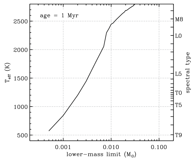
Figure 6: The effective temperature at $a\!=\!1$ Myr from Burrows et al. (1997) with spectral types from Filippazzo et al. (2015). The velocity dispersions for the non-cooling models will be incomplete for spectral types when the lower-mass limit is larger than this relation. For example, the spectral type T5 will be incomplete if the lower-mass limit is set as $m_{0}\!\geq\!0.0015$ M_⊙. However the cooling models will only suffer this incompleteness if there is a significant amount of recent star formation. As discussed in Appendix A, the incomplete velocity dispersions will be biased to older stars and be larger than that of the complete types. Upon experimentation with the lower-mass limit, we find that our velocity dispersions are not substantially affected by our choice of $m_{0}\!=\!0.0005$ M_⊙.

Appendix B Analytic Integration

In the above, we presented a Monte Carlo calculation for predicting the vertical velocity dispersion as a function of spectral type (or effective temperature). We pursued this avenue for analysis so we may make direct comparisons to various published results (e.g. Burgasser, 2004; Deacon & Hambly, 2006; Day-Jones et al., 2013; Burgasser et al., 2015; Marocco et al., 2015), however it is worth mentioning that these Monte Carlo simulations are simply a way of numerical approximating a complex integral. We have verified that our simulations reproduce those published results, but are exactly given by:

$$\left<\sigma^{2}_{w}\right>=\frac{\int\int\psi(t)\,\phi(m)\,\sigma^{2}_{w}(t_{0}-t)\,\Pi(T_{eff}(t_{0}-t,m);T_{0},T_{1})\,\mathrm{d}t\,\mathrm{d}m}{\int\int\psi(t)\,\phi(m)\,\Pi(T_{eff}(t_{0}-t,m);T_{0},T_{1})\,\mathrm{d}t\,\mathrm{d}m}$$ (B1)

where $\Pi(\cdot)$ is the boxcar-windowing function:

$$\Pi(x;x_{0},x_{1})=\begin{cases}0&x<x_{0}\\ 1&x_{0}\leq x\leq x_{1}\\ 0&x_{1}<x,\end{cases}$$ (B2)

and $T_{0}$/$T_{1}$ are the minimum/maximum effective temperature that correspond to a given maximum/minimum spectral type in question, respectively. Equation B1 is similar to the results described by Aumer & Binney (2009), but extended to include atmospheric cooling.

References

- Aumer & Binney (2009) Aumer, M. & Binney J. J. 2009, MNRAS, 397, 1286
- Bahcall (1986) Bahcall, J. N. 1986, ARA&A, 24, 577
- Baraffe & Chabrier (1996) Baraffe, I. & Chabrier, G. 1996, ApJ, 461, L51
- Baraffe et al. (2003) Baraffe, I., Chabrier, G., Barman, T., Allard, F., & Hauschildt, P. H. 2003, A&A, 402, 701
- Best et al. (2017) Best, W. M. J., et al. 2017, arXiv: 1701.00490, ApJ submitted
- Blake, Charbonneau, & White (2010) Blake, C. H., Charbonneau, D., & White, R. J. 2010, ApJ, 723, 684
- Bochanski et al. (2010) Bochanski, J. J., Hawley, S. L., Covey, K. R., West, A. A., Reid, I. N., Golimowski, D. A., & Ivezić, Ž 2010, AJ, 139, 2679
- Bovy & Rix (2013) Bovy, J. & Rix, H.-W. 2013, ApJ, 779, 115
- Burningham et al. (2013) Burningham B., et al., 2013, MNRAS, 433, 457
- Burgasser (2004) Burgasser, A. J., 2004, ApJS, 155, 191
- Burgasser et al. (2015) Burgasser, A. J., et al. 2015, ApJS, 220, 18
- Burrows, Hubbard, & Lunine (1989) Burrows, A., Hubbard, W. B., & Lunine, J. I. 1989, ApJ, 345, 939
- Burrows et al. (1997) Burrows, A., et al. 1997, ApJ, 491, 856
- Caballero, Burgasser, & Klement (2008) Caballero, J. A., Burgasser, A. J., & Klement, R. 2008, A&A, 488, 181
- Chen et al. (2001) Chen, B., et al. 2001, ApJ, 553, 184
- Covey et al. (2007) Covey, K. R., et al. 2007, AJ, 134, 2398
- Day-Jones et al. (2013) Day-Jones, A. C., et al. 2013, MNRAS, 430, 1171
- Deacon & Hambly (2006) Deacon, N. R. & Hambly, N. C. 2006, MNRAS, 371, 1722
- de Grijs & van der Kruit (1996) de Grijs R. & van der Kruit, P. C. 1996, A&AS, 117, 19
- Dehnen & Binney (1998) Dehnen, W. & Binney, J. J. 1998, MNRAS, 298, 387
- Dupuy & Liu (2012) Dupuy, T. J. & Liu, M. C. 2012, ApJS, 201, 19
- Faherty et al. (2009) Faherty, J. K., Burgasser, A. J., Cruz, K. L., et al. 2009, AJ, 137, 1
- Filippazzo et al. (2015) Filippazzo, J. C., Rice, E. L., Faherty, J., Cruz, K. L., van Gordon, M. M., & Looper, D. L. 2015, ApJ, 810, 158
- Hayashi & Nakano (1963) Hayashi, C., & Nakano, T. 1963, Prog. Theor. Phys., 30, 4
- Holwerda et al. (2014) Holwerda, B., et al. 2014, ApJ, 788, 77
- Joergens (2006) Joergens, V. 2006, A&A, 450, 1135
- Jurić et al. (2008) Jurić, M., et al. 2008, ApJ, 673, 864
- Kirkpatrick et al. (2012) Kirkpatrick J. D., et al., 2012, ApJ, 753, 156
- Kumar (1962) Kumar, S. S., 1962, AJ, 67, 579
- Lang (1993) Lang, K. R. 1978, Astrophysical Formulæ, (3rd ed.; Springer-Verlag Berlin Heidelberg)
- Luhman et al. (2006) Luhman, K. L., Whitney, B. A., Meade, M. R., Babler, B. L., Indebetouw, R., Bracker S., & Churchwell, E. B. 2006, ApJ, 647, 1180
- Luhman (2012) Luhman, K. L. 2012, ARA&A, 50, 65
- Marocco et al. (2015) Marocco, F., et al. 2015, MNRAS, 449, 3651
- Masters et al. (2012) Masters, D., et al. 2012, ApJ, 752, L14
- Metchev et al. (2008) Metchev S. A., Kirkpatrick J. D., Berriman G. B., Looper D., 2008, ApJ, 676, 1281
- Moraux & Clarke (2005) Moraux, E. & Clarke, C. 2005, A&A, 429, 895
- Papovich et al. (2015) Papovich, C., et al. 2015, ApJ, 803, 26
- Parker et al. (2011) Parker, R. J., Bouvier, J., Goodwin, S. P., Moraux, E., Allison, R. J., Guieu, S., & Güdel, M. 2011, MNRAS, 412, 2489
- Pirzkal et al. (2005) Pirzkal, N., et al. 2005, ApJ, 622, 319
- Pirzkal et al. (2009) Pirzkal, N., et al. 2009, ApJ, 695, 1591
- Reid et al. (1999) Reid, I. N., et al. 1999, ApJ, 521, 613
- Reid et al. (2002) Reid, I. N., Kirkpatrick, J. D., Liebert, J., et al. 2002, AJ, 124, 519
- Reiners & Basri (2009) Reiners, A., & Basri, G. 2009, ApJ, 705, 1416
- Reipurth & Clarke (2001) Reipurth B & Clarke C. 2001, AJ, 122, 432
- Ryan et al. (2005) Ryan, R. E., Hathi, N. P., Cohen, S. H., & Windhorst, R. A. 2005, ApJ, 631, L159
- Ryan et al. (2011) Ryan, R. E., et al. 2011, ApJ, 739, 83
- Ryan & Reid (2016) Ryan, R. E. & Reid, I. N., 2016, AJ, 151, 92
- Schmidt et al. (2010) Schmidt, S. J., West, A. A., Hawley, S. L., & Pineda, J. S. 2010, AJ, 139,1808
- Seifahrt et al. (2009) Seifahrt, A., Reiners, A., Almaghrbi, K. A. M., & Basri, G. 2009, A&A, 512, A37
- Snaith et al. (2015) Snaith, O., Haywoo, M., Di Matteo, P., Lehnert, M. D., Combes, F., Katz, D. & Gómez, A. 2015, A&A, 578, 87
- Spergel et al. (2015) Spergel, D. et al. 2015, arXiv: 1503.03757
- Spitzer & Schwarzschild (1951) Spitzer, L., Jr., & Schwarzschild, M. 1951, ApJ, 114, 385
- Stephens et al. (2009) Stephens, D. C., et al. 2009, ApJ, 702, 154
- van der Kruit (1988) van der Kruit, P. C. 1988, A&A, 192, 117
- van Vledder et al. (2016) van Vledder, I., van der Vlugt, D., Holwerda, B. W., Kenworthy, M. A., Bouwens, R. J., & Trent, M. 2016, MNRAS, 458, 425
- Wielen (1977) Wielen, R. 1977, A&A, 60, 263
- White & Basri (2003) White, R. J. & Basri, G. 2003, ApJ, 582, 1109
- Yan, Windhorst, & Cohen (2003) Yan, H., Windhorst, R. A., & Cohen, S. H. 2003, ApJ, 585, L93
- Zapatero Osorio et al. (2007) Zapatero Osorio, M. R., Martín E. J., Béjar, V. J. S., Bouy, H., Deshpande, R., & Wainscoat, R. J. 2007, ApJ, 666, 1205
- Zheng et al. (2001) Zheng, Z., Flynn, C., Gould, A., Bahcall, J. N., & Salim, S. 2001, ApJ, 555, 393