X-ray morphological analysis of the Planck ESZ clusters

Abstract

X-ray observations show that galaxy clusters have a very large range of morphologies. The most disturbed systems which are good to study how clusters form and grow and to test physical models, may potentially complicate cosmological studies because the cluster mass determination becomes more challenging. Thus, we need to understand the cluster properties of our samples to reduce possible biases. This is complicated by the fact that different experiments may detect different cluster populations. For example, SZ selected cluster samples have been found to include a greater fraction of disturbed systems than X-ray selected samples. In this paper we determined eight morphological parameters for the Planck Early Sunyaev-Zeldovich (ESZ) objects observed with XMM-Newton. We found that two parameters, concentration and centroid-shift, are the best to distinguish between relaxed and disturbed systems. For each parameter we provide the values that allow one to select the most relaxed or most disturbed objects from a sample. We found that there is no mass dependence on the cluster dynamical state. By comparing our results with what was obtained with REXCESS clusters, we also confirm that indeed the ESZ clusters tend to be more disturbed, as found by previous studies.

1 Introduction

Galaxy clusters were first detected as high concentrations of galaxies in the sky. In addition to the galaxies, there is a hot X-ray emitting intracluster medium (ICM) that accounts for the bulk of the cluster baryons. That makes X-ray surveys a powerful tool for cluster detection. More recently, Sunyaev-Zeldovich (SZ, Sunyaev & Zeldovich 1972) observations have opened a new window for cluster detection and are now providing new catalogs. Due to the different dependence of the SZ and X-ray emission on the gas density, there is currently a debate regarding whether the two experiments are detecting the same population of galaxy clusters. In particular, since the X-ray emission scales with the square of the gas density, X-ray surveys are more prone to detect centrally peaked, more relaxed galaxy clusters (e.g. Eckert et al. 2011). Being less sensitive to the central gas density the SZ experiments detect more unrelaxed clusters (e.g. Planck Collaboration et al. 2011a).

The first indications that dynamically disturbed objects are more represented in the SZ than X-ray surveys were found by Planck Collaboration et al. (2011a) and Planck Collaboration et al. (2013) by comparing the scaled density profiles of the newly-detected SZ clusters with the ones of REXCESS clusters, a representative X-ray sample. The SZ objects have on average flatter gas density distributions (i.e. are more disturbed morphology). Recently Rossetti et al. (2016) used the projected distance between the X-ray peak and the BCG as an indicator of relaxation for galaxy clusters. They found that X-ray selected samples tend to be more relaxed than SZ selected clusters and they interpreted the result as an indication of the cool core bias. In a second paper, Rossetti et al. (2017) also investigated another morphological parameter (concentration) and they confirmed their first paper’s result and they supported the cool core bias interpretation by performing a set of simulations. The result has been also confirmed by Andrade-Santos et al. (2017) who compared the concentration, cuspiness and central density for the ESZ sample (only the clusters with redshift lower than 0.35) and an X-ray flux limited sample. Although both papers obtained similar results, they provide a different explanation for the selection effects. Andrade-Santos et al. (2017) described a simple model which predict that cool core clusters are over-represented in X-ray samples because of the Malmquist bias and were able to reproduce their results just considering the average luminosity difference between cool core and non cool core clusters. Rossetti et al. (2017) performed a set of dedicated simulations by considering the different shape of the surface brightness profile for cool core and non cool core clusters to produce a realistic population of galaxy clusters and investigate the effect of the X-ray and SZ selection. They found that Malmquist and CC biases are probably at the origin of the different fraction of relaxed systems in the two samples but unlikely it can explain the whole difference. The above-mentioned papers are based on Planck selected samples while, interestingly, Nurgaliev et al. (2017), via two other methods (i.e. centroid shifts and photon asymmetry), did not find significant differences in the observed morphology of X-ray and SPT selected samples. On the other hand, the different papers also used different X-ray samples (with different redshift and mass properties, as well as selection methods) for the comparison which complicate the interpretation of the different results as discussed in more detail by Rossetti et al. (2017).

The different fractions of relaxed and unrelaxed systems in the samples have important implications for cosmology. In fact, the cluster mass, which is the most fundamental property to use clusters for cosmological studies, can be over- or underestimated during a cluster merger when clusters are generally not in hydrostatic equlibrium (e.g. Randall et al. 2002). Moreover, compression and heating can alter both temperature and luminosity (e.g. Ricker & Sarazin 2001). Even for relaxed systems, accurate determination of the mass requires good knowledge of both the gas density and temperature profiles up to $R_{500}$, which are not available for many systems. And in the future almost all groups and clusters detected with eROSITA will have too few photons to measure their temperature and mass profiles (Borm et al. 2014). Thus, cosmological studies using groups and clusters of galaxies rely heavily on a detailed understanding of the scaling relations. Measures of the dynamical states of the systems offer important information to obtain precise scaling relations and understand their scatter. For example, Mantz et al. (2015) showed that the identification of substructure in galaxy clusters allowed an accurate selection of relaxed systems that led to tight constraints on the cosmological evolution of the gas mass fraction. Moreover, although to test the cosmological models we need the mass function of the whole population, the X-ray masses, obtained under the assumption of HE are more robust for relaxed clusters (e.g. Rasia et al. 2006, Lau et al. 2009). A recent study by Applegate et al. (2016) based on relaxed systems disfavor strong departures from hydrostatic equilibrium and show a good agreement between X-ray and lensing masses (see also the results by Israel et al. 2014). Andrade-Santos et al. (2012) showed that since disturbed systems tend to be less luminous and less massive they can be used in the scaling relations once the level of substructures is known and parametrized so that their positions in the mass-observable planes can be corrected (e.g. Ventimiglia et al. 2008). Opposed to the cosmological studies, astrophysical investigations usually focus more on highly disturbed galaxy clusters where phenomena like turbulence and particle (re-)acceleration are more prominent and easier to be investigated. Furthermore, most of these disturbed galaxy clusters are outliers in many scaling relations, thus their identification is fruitful for many different studies.

To characterize the dynamical state of a galaxy cluster requires access to a large set of information in different wavelengths (e.g. gas thermodynamical properties distribution from X-ray data; total mass distribution from the lensing analysis) which are available only for a few individual clusters. An alternative is to compute well defined morphological parameters, making use of the relatively cheap X-ray images and profiles. Several morphological indicators have been proposed in the last few decades: e.g., BCG-X-ray peak offset (e.g. Jones & Forman 1984, Jones & Forman 1999), centroid shifts (Mohr et al., 1993), power ratios (Buote & Tsai, 1995, 1996), concentration parameter (Santos et al., 2008), and photon asymmetry (Nurgaliev et al., 2013). Pinkney et al. (1996) and Böhringer et al. (2010) showed that because of the different projection effects, none of these methods is good in all cases and a combination of them might be more effective to quantify the level of substructures. Thus, given the large amount of new data that will be collected from current and future surveys, and that both X-ray and SZ detection methods may have some common biases (Angulo et al. 2012; Lin et al. 2015), it is important to investigate the morphological indicators for large cluster samples and i) identify which parameter(s) most efficiently allow us to classify relaxed and disturbed objects, and ii) verify if the X-ray morphologies of X-ray and SZ samples are consistent.

The subdivision of relaxed and disturbed systems is itself very hard because there is no rigorous definition and a simple subdivision into two classes is probably over-simplistic. In fact, the measure of the level of relaxation of galaxy clusters as given by the morphological parameters is a continuos function, from very relaxed systems (i.e. objects with circular X-ray isophotes and without substructures) to very disturbed objects (i.e. clear evidence of merging). While most of the systems are not on the tail of the distribution, as discussed above, several studies are only interested on the extreme systems (either the most relaxed or the most disturbed). Thus, instead of finding parameter values that split the objects in two subsamples, for these studies, it is more important to have threshold values that selectively exclude most, if not all, the relaxed or unrelaxed systems.

In this paper we study a set of 8 morphological parameters. Some of them are derived from the X-ray images, while others are derived from the surface brightness (SB) and electron density profiles. The goal is to identify which are the best parameters to pinpoint the most relaxed and most disturbed galaxy clusters.

We assume a $\Lambda$CDM cosmology with $H_{0}$=70 km/s/Mpc, $\Omega_{\Lambda}$=0.7 and $\Omega_{m}$=0.3. The outline of the paper is organized as follows. In §2 we present the data preparation and analysis. The definitions of the morphological parameters are presented in §3 and the results in §4. In §5 and §6 we discuss the results and present our conclusions.

2 Data analysis

2.1 The sample

Simulations have shown that the SZ quantities weakly depends on the dynamical state of the objects (e.g. Motl et al. 2005) suggesting that SZ selected samples might be more representative of the underlying cluster population and so more appropriate for the study we are carrying out in this paper.

ESA’s Planck Mission has provided a long list of cluster candidates from which two large and statistically representative samples have been extracted: i) the ESZ sample (Planck Collaboration et al. 2011b), and ii) the PSZ1 cosmology sample (Planck Collaboration et al. 2014). Both samples would be suitable for our analyses but we choose the ESZ sample because when we started this analyses (beginning of 2016) its XMM-Newton coverage (public data for 149 vs 142 clusters, respectively) was larger than for the PSZ1 cosmological sample.

The ESZ sample consists of 189 massive clusters (one is a false detection), by imposing a signal-to-noise ratio threshold of 6 on the catalogue of Sunyaev-Zel’dovich (SZ) detections above the Galactic plane ($|b|>15^{\circ}$). The clusters span a quite broad redshift range, from 0.01 to 0.55. XMM-Newton has observed 155 of these Planck clusters, but for five of them the observations are completely flared and cannot be used for the characterization of the cluster properties.

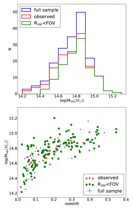
Figure 1: top: Distribution of the Planck cluster masses within $R_{500}$ for the ESZ sample. The blue histogram refers to all the 188 objects, the red histogram to the clusters observed with XMM-Newton (excluding the flared observations), and the green histogram to the clusters that completely fit within the XMM-Newton FOV. bottom: Mass-redshift distribution for the ESZ sample with the same colors are in the top panel.

2.2 Data reduction

Observation data files (ODFs) were downloaded from the XMM-Newton archive and processed with the XMM v.16.0.0 software for data reduction. The initial data processing to generate calibrated event files from raw data was done by running the tasks emchain and epchain. We only consider single, double, triple, and quadruple events for MOS (i.e. PATTERN$\leq$12) and single for pn (i.e. PATTERN==0), and we applied the standard procedure for the removal of bright pixels and hot columns (i.e. FLAG==0) and the pn out-of-time correction. All the data were cleaned for periods of high background due to the soft protons, following the procedure extensively described in Lovisari et al. (2015).

2.3 Image analyses

The X-ray images were created in the 0.3-2 keV energy band to maximize the signal-to-noise using a binning of 82 physical pixels corresponding to a resolution of 4.1 arcsec. The background subtraction was performed using a combination of blank-sky field (BSF) and filter wheel closed (FWC) observations as described in Lovisari et al. (2011). Briefly, we selected the data sets with the most similar background properties for each cluster. We filtered the events by applying the same selection criteria used for the observations. For each detector we added/subtracted the renormalized FWC observations to the corresponding BSF images to compensate for the difference between the out-of-field-of-view (OOFOV) events (which are a good indicator of the level of the particle background) in the observation and in the BSF data. The normalization factors were obtained by fitting the OOFOV events of both the observation and the BSF in the 3-10 keV energy band (for more details about this choice see Zhang et al. 2009) with a model that includes a power-law and several gaussian lines to account for the fluorescent emission observed in both detectors. The normalization factors were derived as the ratio of the powerlaw normalization of the observation to the BSF. The data from the three detectors were combined into a single image and divided by the combined exposure map after the MOS exposures were rescaled by a factor to account for the difference in effective area. The weighting factors have been obtained by determining the scaling of the cluster surface brightness profiles observed with each of the three detectors (see Böhringer et al. 2010). Thanks to this procedure all the gaps (e.g. CCD gaps) are removed from the final images. Regions exposed with less than 5$\%$ of the total exposure were excluded
Point-like X-ray sources were detected with the edetect-chain task and visually inspected to discriminate between real point sources and extended cluster substructures. The latter were not removed from the data files. After removing the point sources, the holes were refilled using the CIAO task dmfilth.

2.4 Surface brightness

We determined the surface brightness (SB) profiles, centered on the X-ray peak of the main cluster component, from the background-subtracted, vignetting-corrected images, as described in the previous section. The chosen energy band provides an optimal ratio of the source over background flux for XMM-Newton data and ensures an almost temperature-independent X-ray emission. For the calculation of the profiles, to avoid “humps” in the SB profiles due to the presence of substructures or a secondary peak (e.g. in the case of an infalling system), we removed all substructures clearly visible by eye. For bimodal mergers, the profiles were obtained independently for the two subclusters. The SB profiles were fitted with a double $\beta$-model:

$$S_{X}(r)=\sum\limits_{i=1}^{2}S_{0,i}\left[1+\left(\frac{r}{r_{c,i}}\right)^{2}\right]^{-3\beta+0.5}$$ (1)

where $r_{c,i}$ and $S_{0,i}$ are the core radius and central surface brightness of each of the two components, respectively. This model usually provides a good fit for all the clusters once the main substructures are removed.

2.5 $R_{500}$

Galaxy clusters are at the nodes of the cosmic web, so at large radii they are expected to show signatures of accretion processes (e.g. Roncarelli et al. 2006). Hydrodynamical simulations have shown that within $R_{500}$, galaxy clusters are relatively relaxed unless a merger event modifies the existing conditions. Thus, $R_{500}$ represents the optimal radius for the morphological analysis to obtain a comprehensive view of the dynamical state of the clusters. Due to their low redshifts, a small fraction of objects do extend beyond the XMM-Newton FOV, so we also computed the morphological parameters within 0.5$R_{500}$.
Using the spectral temperature, $T_{init}$, measured in the region that maximizes the signal-to-noise in the 0.3-2 keV band, we estimated an initial $R_{500,init}$ using the equation from Arnaud et al. (2005):

$$R_{500,init}=1.104\times(T_{init}/5\ {\rm keV})^{0.57}E(z)^{-1}$$ (2)

where E(z) is the ratio of the Hubble constant at redshift z to its present day value. We then calculated the total gas mass ($M_{gas}$) by integrating the density profile within that radius and computed $Y_{X}$=$M_{gas}{\times}T_{init}$. By using the $M$-$Y_{X}$ relation given in Arnaud et al. (2010), assuming self-similar evolution,

$$E(z)^{0.4}M_{500}=10^{14.567}\left[\frac{Y_{X,500}}{2\times 10^{14}M_{\odot}keV}\right]^{0.561}M_{\odot}$$ (3)

we estimate $M_{500}$ and $R_{500}$. We then re-extracted a spectra in the region within 0.15-0.75$R_{500}$ to determine a new temperature and re-computed $Y_{X}$ using the new $R_{500}$ and $M_{500}$. The procedure is repeated until convergence, which happens when the difference between the initial and the new temperature is smaller than 1$\%$.

The spectral analysis were done using XSPEC (Arnaud, 1996). All the spectra were re-binned to ensure at least 25 counts per bin and a minimum energy width per bin of 1/3 of the full width half maximum (FWHM) to prevent to oversample the instrument spectral resolution. Spectra were fit in the 0.3-10 keV energy range with an absorbed APEC (Smith et al. 2001) thermal plasma with a column density from Willingale et al. (2013). The EPIC spectra were fitted simultaneously, with temperatures and metallicities linked and enforcing the same normalization value for MOS, and allowing the pn normalization to vary.

3 Morphological parameters

In the following we introduce the methods for the substructure and morphology characterization.

3.1 Concentration

The concentration parameter indicates how concentrated the X-ray emission is and was first introduced by Santos et al. (2008) as a good indicator for the presence of cooling core systems at high redshift. It is defined as the ratio of the emission within 2 different circular apertures. In this paper we use:

$$c=\frac{SB(<0.1R_{500})}{SB(<R_{max})}$$ (4)

where R_max can be either 0.5R₅₀₀ or R₅₀₀. While in papers using Chandra observations, it is possible to use directly the source counts estimated from the images, here we must take into account the XMM-Newton PSF. Thus, we integrated the SB profiles deconvolved with the PSF. We discuss the relation between the concentration value obtained with and without the PSF correction in Appendix B.

3.2 Centroid shift

The centroid shitft parameter is defined as the variance of the projected separation between the X-ray peak determined from the smoothed image (with a Gaussian of FWHM of 6 arcsec) and the centroid of the emission obtained within 10 apertures of increasing radius up to $R_{max}$:

$$w=\left[\frac{1}{N-1}\sum_{i}(\Delta_{i}-\overline{\Delta})^{2}\right]^{\frac{1}{2}}\frac{1}{R_{max}}$$ (5)

The default value for $R_{max}$ is $0.5R_{500}$, but when R₅₀₀ fits completely within the FOV we also estimated the values at $R_{max}=R_{500}$.

3.3 Power ratios

Introduced by Buote & Tsai (1995), the power ratio method is motivated by the idea that the SB is a good representation of the projected mass distribution of the cluster. The power ratios consist of a 2D multipole decomposition of the surface brightness distribution within a specified aperture and they account for the radial fluctuations where the high order moments are sensitive to smaller and smaller scales.
The m-order power ratio is defined as $P_{m}/P_{0}$ with

$$P_{0}=[a_{0}\ln(R_{ap})]^{2}$$ (6)

$$P_{m}=\frac{1}{2m^{2}R_{ap}^{2m}}(a_{m}^{2}+b_{m}^{2})$$ (7)

where $a_{0}$ is the total intensity within the aperture radius $R_{ap}$. The moments $a_{m}$ and $b_{m}$ are calculated by

$$a_{m}(R)=\int_{R<R}S(x)R^{m}\cos(m\phi)d^{2}x$$ (8)

and

$$b_{m}(R)=\int_{R<R}S(x)R^{m}\sin(m\phi)d^{2}x$$ (9)

where S(x) is the X-ray surface brightness at the position x=(R,$\phi$). In this paper we focus on the third (i.e. P3/P0, hereafter P30) and fourth (i.e. P4/P0, hereafter P40) moments which are sensitive to the large and small scale substructures.

3.4 Gini coefficient

The Gini coefficient, a standard economic measure of income inequality, was used for the first time in astronomy by Abraham et al. (2003) to measure the light concentration of all galaxy types and characterize their morphology. In this paper we use it as a measure of the X-ray flux distribution in galaxy clusters. If the total flux is equally distributed among the considered pixels, then the Gini coefficient is equal to 0, while if the total flux is concentrated into a single pixel, then its value is equal to 1. We adopt the definition from Lotz et al. (2004):

$$G=\frac{1}{|\bar{K}|n(n-1)}\sum_{i}(2i-n-1)|{K_{i}}|$$ (10)

where $K_{i}$ is the pixel value in the i-th pixel of a given image, n is the total number of pixels, and $\bar{K}$ is the mean of the absolute values of all n pixels in the image. As discussed by Lotz et al. (2004), the absolute values of $k_{i}$ are required because in the low surface brightness regions some pixels can result in negative values after the background subtraction. Including those negative values can yield a Gini coefficient to achieve values higher than 1. We note that the Gini coefficient is less sensitive to surface brightness effects and does not require a well-defined centroid (i.e. whether the flux is concentrated into a few pixels in the center or in the outer regions the obtained value is the same). That makes this parameters interesting for distant clusters and shallow observations that do not allow a precise determination of the X-ray peak. To our knowledge only Parekh et al. (2015) computed this parameter to X-ray observations of galaxy clusters.

3.5 Central electron density

While the formation of a cool core in the ICM is not a fully understood process, many studies (e.g. Hudson et al. 2010) have shown that the most relaxed systems tend to have a high gas density core with no significant redshift evolution (e.g. McDonald et al. 2017). Under the assumption of spherical symmetry, the gas density profile can be obtained from the combination of the best-fit results from the spectral and imaging analyses as described in Lovisari et al. (2015) (see also Hudson et al. 2010). In this paper we use the value of the density computed at 0.02$R_{500}$ to avoid the problem with the modeling close to R=0 (where the density profile may diverge) but still close enough to the cluster center to be representative of the central electron density. The central densities have not been scaled by E(z)${}^{-}2$ but given the small redshift range the impact to the values is modest.

3.6 Cuspiness

Related to the density profile the cuspiness was suggested by Vikhlinin et al. (2007) and it is defined as:

$$\alpha=-\frac{d\log\rho_{g}}{d\log r}$$ (11)

where $\rho_{g}$ is the gas density profile and the function is computed at a fixed scaled radius of 0.04$R_{500}$. This radius was chosen to be close enough to the core that the effect of cooling is strong but far enough to avoid the flattening of the profile due to the outflows from the central AGN. We note that although for the SB profiles we removed most of the substructures there are still a few cases where the fit is not perfectly in agreement with the data points which might bias the cuspiness for some of the clusters (in particular the most disturbed ones).

3.7 Ellipticity

Although not necessarily a measure of substructures, the ellipticity is commonly defined by the ratio between the semi-minor and semi- major axis. A measure of the ellipticity can also be obtained by the power ratio P2/P0. Although we verified that the two measurements are well correlated, in this paper we used the first definition.

4 Results

Of the 150 analyzed clusters (excluding the ones with completely flared observations), 120 clusters have $R_{500}$ completely within the XMM-Newton field-of-view. For 28 clusters, the estimated $R_{500}$ extends beyond the FOV, but we could still measure their properties within 0.5$R_{500}$. Two of the analyzed objects (AWM7 and A1060) are very nearby and therefore only a small fraction of their radius (i.e. $<$0.3$R_{500}$) lies within the FOV. Therefore, we excluded them from the analysis. Thus, when plotting the parameters determined within $R_{500}$, we only use 120 objects, while when we investigate the properties at $0.5R_{500}$, we make use of the full sample of 148 objects. The subsample of objects observed with XMM-Newton is representative of the full sample in terms of total masses (see top panel of Fig. 1). The same is true for the objects fitting the XMM-Newton FOV although the full sample includes a tail of low mass objects. In the bottom panel of Fig. 1 we also show the Planck mass-redshift distribution of the objects in the ESZ sample and the XMM-Newton coverage.

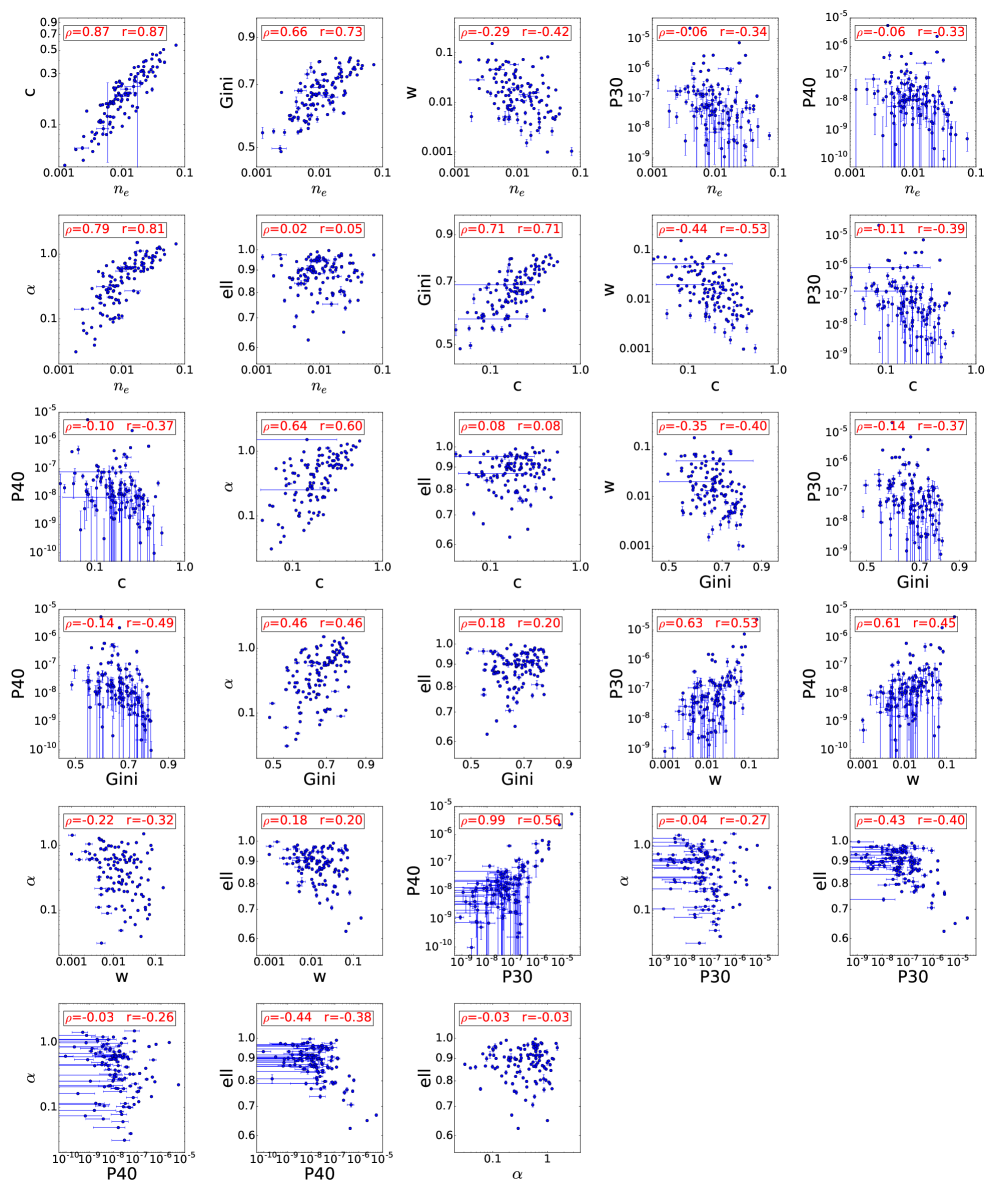
Figure 2: Parameters obtained within $R_{500}$ plotted in the parameter-parameter planes. Here we show only the 120 galaxy clusters that have $R_{500}$ completely within the XMM-Newton FOV. The $\rho$ and r values indicate the Pearson and Spearman correlation coefficient (note that r is computed on ranks and so characterizes monotonic correlations, while $\rho$ is on true values and characterizes linear correlation). Some of the parameters show a clear and strong correlation while others are much more scattered.

4.1 Morphology parameters

The results of the substructure analysis is summarized in Fig. 2 where we report the distribution of the parameters calculated within $R_{500}$ (see Appendix C for the parameters calculated within 0.5$R_{500}$). The uncertainties of the morphological parameters obtained directly using the images (i.e. Gini coefficient, centroid-shift, power-ratios, and ellipticity) have been obtained via monte-Carlo simulations as previously done by Cassano et al. (2010) and Donahue et al. (2016). For every cluster we simulated 100 versions of the X-ray images by resampling the counts per pixel according to their Poissonian error. Similarly, to obtain the uncertainties of the parameters associated with the profiles (i.e. $n_{e}$, cuspiness, and concentration), we randomly varied the observational data points of the SB profiles 100 times to determine a new best fit. Again, the randomization was driven from the Gaussian distribution with mean and standard deviations in accordance with the observed data points and the associated uncertainties. Apart from the power ratios the uncertainties are very small (see Table H1) and they are not expected to play a big role in the correlations and classification scheme for which we used only the parameter values. Thus, the errors have been used only for illustration purposes.

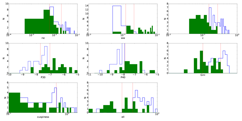
Figure 3: Distribution of the relaxed (blue) and disturbed (green) systems as a function of the different parameters. The vertical red lines represent the limit values used in Tables 2 and 3. To highlight the difference between relaxed and disturbed systems the “mix” objects are not plotted.

Although the different plots show a significant intrinsic scatter, the expected correlation between several parameters can still be observed. In fact, large centroid shifts and power-ratios, as well as small X-ray concentrations, Gini coefficients, and central densities are likely associated with disturbed clusters and so these measurements are expected to correlate with each other. The strongest correlations (see Table I1 in the Appendix) have been obtained by comparing parameters that are more sensitive to the core properties like for example c-n_e ($\rho$=0.87 and r=0.87), c-Gini ($\rho$=0.71 and r=0.71), or Gini-n_e ($\rho$=0.66 and r=0.73). A good correlation is also obtained when comparing parameters that are more sensitive to the level of substructures, e.g. w-P30 ($\rho$=0.63 and r=0.53), w-P40 ($\rho$=0.61 and r=0.45), or P30-P40 ($\rho$=0.99 and r=0.56). A weaker correlation instead is found when comparing a parameter sensitive to the core properties with one parameter sensitive to the level of substructures (e.g. $n_{e}$-w ($\rho$=-0.29 and r=-0.42), $c$-P30 ($\rho$=-0.11 and r=-0.39), or Gini-P40 ($\rho$=-0.14 and r=-0.49)).The ellipticity, while showing no correlation with the parameters sensitive to the core properties, correlates with the ones sensitive to the level of substructures.

4.2 Finding the most relaxed and most disturbed objects

Each parameter has a different ability to distinguish between relaxed and unrelaxed systems. To evaluate each parameter’s ability in determining the dynamical state we follow a procedure presented by Rasia et al. (2013) where the clusters are visually classified as relaxed, disturbed and “mix”. A group of six astronomers inspected the images and rated the relaxation state of the clusters with a grade that ranges from 1 (most relaxed) to 4 (most disturbed). We then averaged the results. All the clusters with an average grade lower than 2 were classified as relaxed while the clusters with an average grade larger than 3 were classified as disturbed. We refer to the remaining clusters with grade from 2 to 3 as “mix”. Although the classification is subjective, broadly speaking, objects with circular X-ray isophotes and without substructures are classified as relaxed, double or complex objects with clear evidence of merging are classified as disturbed, and all the other with small substructures or relatively flat X-ray distribution as “mix” objects (see the cluster images in the Appendix). The distribution of relaxed and unrelaxed objects are significantly shifted with little overlap for the centroid-shift, concentration, and power ratio parameters (see Fig. 3). The overlap is larger for the central density, Gini, cuspiness and ellipticity. For these latter parameters, choosing a threshold value to classify the objects will lead either to a contaminated or incomplete sample. By “contaminated” we mean that some of the disturbed systems will be classified as relaxed (or the reverse), while for “incomplete”, we mean that some of the relaxed objects are not recognized. If two distributions would completely shift apart, then one can choose the threshold value that allows to have a complete and not contaminated sample. However, since all the histograms overlap, one needs to find a good compromise between the completeness of the sample and its contamination. Following Rasia et al. (2013), we define two properties, the sample completeness “C” and the purity “P”:

$$C_{r}=\frac{QN(relaxed)}{TN(relaxed)}$$ (12)

$$P_{r}=\frac{QN(relaxed)}{QN(relaxed+disturbed)}$$ (13)

where QN is the number of objects above (or below) a certain threshold and TN is the total number of objects. In a similar way we computed $C_{d}$ and $P_{d}$ for the disturbed objects. We also provide the purity of the sample when “mix” objects are also considered:

$$P_{ext}=\frac{QN(relaxed)}{QN(relaxed+disturbed+mix)}.$$ (14)

In Table 1 we summarized the results of the analyses where we searched for the threshold values that optimize either C or P. The two cluster parameters that perform better to select the relaxed systems are the concentration and the centroid shift that, for a completeness of 100$\%$ both have a purity of 84$\%$. The centroid shift performs better than the concentration if one searches for high purity (e.g. P$>95\%$). In fact the high purity for the concentration is reached of the higher detriment of the completeness than for the centroid-shift. The selection of the most disturbed objects results more difficult than for the relaxed objects. This is probably due to the fact that parameters that depend on models, like c or $n_{e}$, are better determined for relaxed than disturbed clusters. The clusters marked as disturbed but showing a rather high concentration (see Fig. D1) are usually double or complex objects. For those clusters only the main subscluster was used for the calculation of the concentration values, slightly overestimating the concentration. The centroid shift results again the best parameter to distinguish the most disturbed objects from the most relaxed but the purity of the sample is lower.

The different parameters are sensitive to different properties of the clusters. For example power-ratios and centroid shifts are sensitive to the presence of substructures, while the central density is more connected to the core properties of the clusters. Due to that some objects, which are quite relaxed and peaked in the center with some infalling substructures, can be classified differently if one use different parameters. One way to have a more robust selection of the most relaxed clusters in the sample is to combine more parameters. When combining two parameters, we want to keep the completeness as high as we have done with one single threshold but increase the purity of the sample. For example, for both concentration and centroid shift taken individually, the chosen thresholds give a 100$\%$ completeness, but “only” a 84$\%$ purity. Combining concentration and centroid-shift we obtain a purity of 97$\%$, while maintaining the full completeness. In general adding a second parameter in the selection of the relaxed clusters always improves the purity of the sample although for some, the completeness drop below 90$\%$. In Table 2 we list only the best combination of parameters. The centroid shift does a very good job in removing unrelaxed objects from the sample. In fact, the purity of all the parameters increases by 10$\%$ or more when combined with w. Also the power-ratios and ellipticity help to increase the purity of the sample although not as significantly as the centroid shift. This suggests that combining a parameter more sensitive to the level of substructures like w, P30, and P40 with parameters that are more sensitive to the core properties like $n_{e}$ and c is the best way to identify the most relaxed clusters.

Combining more than two morphological parameters usually reduces the completeness of the sample. For example, the only combination of three parameters that maintains the full completeness of relaxed clusters is c$>$0.15, w$<$0.021, and P30$<$2E-7. However, that removes only very few “mix” objects.

Table 1: For each parameter we indicate the limit (L) that characterize the relaxed and disturbed systems and the purity (P) and completeness (C) parameters. P_ext refers to the purity calculated including the “mix” objects. For most of the parameters we provide two threshold values, one to optimize the completeness and one to optimize the purity.

Par	relaxed				disturbed
	Lr	Cr	Pr	Pext	Ld	Cd	Pd	Pext
$n_{e}$		$>$7.0e-3	0.97	0.74	0.45	$<$3.1e-2	1.00	0.49	0.27
$n_{e}$	$>$2.5e-2	0.32	0.92	0.71	$<$7e-3	0.54	0.94	0.39
$w$	$<$2.1e-2	1.00	0.84	0.48	$>$1.2e-2	0.96	0.79	0.40
$w$	$<$1.2e-2	0.82	0.97	0.60	$>$2.1e-2	0.75	1.00	0.51
$c$	$>$0.15	1.00	0.84	0.47	$<$0.27	1.00	0.61	0.31
$c$	$>$0.27	0.53	1.00	0.67	$<$0.15	0.75	1.00	0.60
Gini	$>$0.6	0.95	0.69	0.38	$<$0.75	1.00	0.54	0.27
Gini	$>$0.74	0.45	0.94	0.68	$<$0.60	0.43	0.86	0.46
P30	$<$2.0e-7	1.00	0.75	0.40	$>$2.0e-8	0.93	0.57	0.29
P30	$<$2.0e-8	0.47	0.90	0.58	$>$2.0e-7	0.54	1.00	0.63
P40	$<$5.0e-8	0.97	0.71	0.39	$>$5.0e-9	0.93	0.58	0.29
P40	$<$1.0e-8	0.68	0.87	0.65	$>$5.0e-8	0.46	0.93	0.54
cusp	$>$0.10	0.97	0.64	0.34	$<$1.00	0.93	0.44	0.24
ell	$>$0.84	0.97	0.67	0.40	$<$0.95	0.82	0.40	0.32

Table 2: For each parameter we indicate the limit (L) that characterize the relaxed and disturbed systems and the purity (P) and completeness (C) parameters. We list here only the combination of parameters that gives the best results. As in Table 2 P_ext refers to the purity calculated including the “mix” objects.

Samples of SZ selected clusters tend to be more dynamically disturbed (i.e. high centroid shift and low concentration and central density) than the X-ray selected samples in agreement with what has been found by other recent studies.

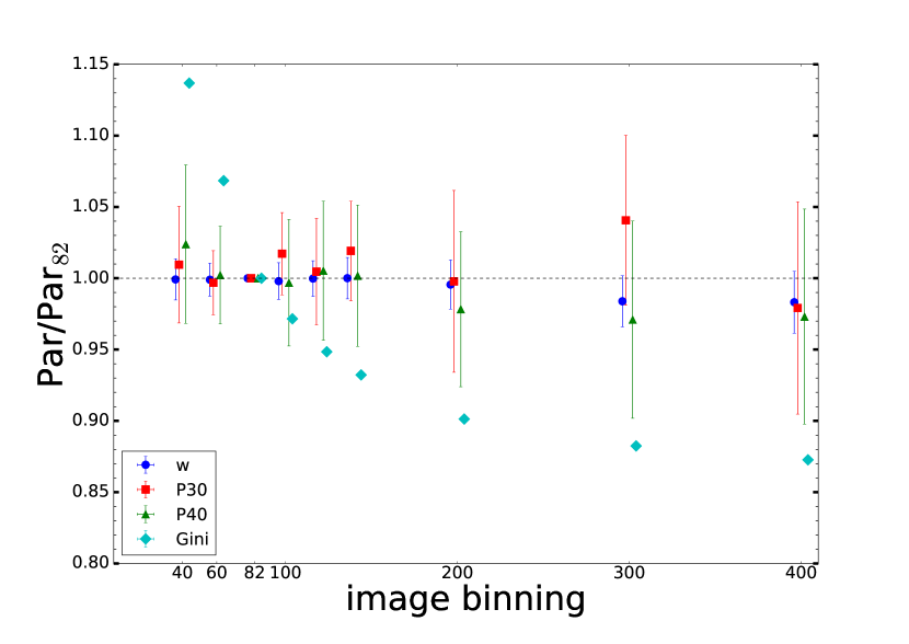
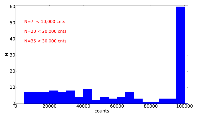
Figure A1: left: The relative change of the the centroid-shift (blue), P30 (red), P40 (green) and Gini (cyan) for different image binning with respect to the nominal binning (82 pixels corresponding to 4.1^′′). The image binning has little impact on all the morphological parameters, except the Gini coefficient. right: Distribution of the galaxy clusters as a function of the number of counts within $R_{500}$. In the last bin we included all the objects with more than 100,000 counts. The legend report how many objects are below a certain threshold.

Appendix A Robustness of the parameters

The clusters in our sample cover a large redshift range so their extension on the sky varies from object to object, which might introduce systematic uncertainties in our measurements. In fact, for more distant objects, it might be harder to measure the small scale substructures. Moreover, if the same image binning is used, for clusters at different redshift we will probe a different physical scale. Furthermore, while some clusters have been observed with very long exposures, others have been observed with relatively short observations. This, can introduce an uncertainty in the determination of the X-ray peak (in particular for the most unrelaxed objects) because of the poorer statistic, and reduce our ability to detect the smaller and fainter substructures. In this section we describe the tests we performed to ensure that our results are stable and robust. First, we checked how important is the choice of the image binnings on the estimated parameters. Indeed, that choice has no impact on the parameters determined using the SB profiles (e.g. central density or concentration) but may play a role for the parameters derived using the images. In Fig. A1 we show the results for 7 different binning. The centroid shift, being basically a measure of the flux distribution, is insensitive to the choice of the binning. This is very important when comparing clusters at different redshifts. The power ratios, which are a measure of the surface brightness inhomogeneities were expected to be a bit more sensitive to the choice of the image binning. In particular one would have expected to find lower values (i.e. more relaxed objects) when a higher binning is used, but the results in Fig. A1 show that this is not the case and also that the power ratios are robust and independent of the choice of binning (if that would not have been the case, we would have found more relaxed objects at high redshift due to the different physical space probed by the same binning). The Gini coefficient instead shows a trend with the binning. In particular increasing the binning leads to a lower Gini coefficient. This happens because a larger binning tends to homogenize the flux distribution over the considered pixels. In fact, conceptually Gini is computed by ordering the pixels in ascending order by flux (or counts) and then comparing the resulting cumulative distribution to what would be expected if all the pixels would have the same flux. So, when the flux difference from pixel to pixel is reduced, the cumulative distribution tends to deviate less from a perfectly even flux distribution. As a consequence of that and given the fact that we used a constant binning for our X-ray images, the obtained Gini factors for high redshift clusters tend to be biased low with respect to the low redshift objects.

To test if the different exposures of the clusters in our sample can systematically bias our results, we recomputed the morphological parameters for all the objects reducing the observation times by 50$\%$, 80$\%$, 90$\%$, and 95$\%$, respectively. Again, we found that the centroid shift is not sensitive to the quality of the data and the correct value can be recovered with relatively short observations. Indeed, the longer the observations, the smaller are the statistical errors associated with the measurements. The power ratios are more sensitive to the number of source counts. For example, Weißmann et al. (2013) showed that relaxed clusters appear more disturbed if the number of counts is significantly less of 30,000 counts. In general our clusters have a very good statistic with only a few clusters below 10,000 source counts (see the histogram in Fig. A1). But applying a counts cut to our sample does not improve significantly the completeness and the purity of the sample. For example if we exclude all the objects with less than 30,000 counts, our completeness for P30$<$1E-7 increases from 90$\%$ to 93$\%$ and the purity from 79$\%$ to 84$\%$. We note that the X-ray peaks determined with a different fraction of the exposure time agree within a few arcsec for all the objects and that the scatter of the parameter values due to that difference in the uncertainty of the cluster center is negligible, if compared with the errorbars.

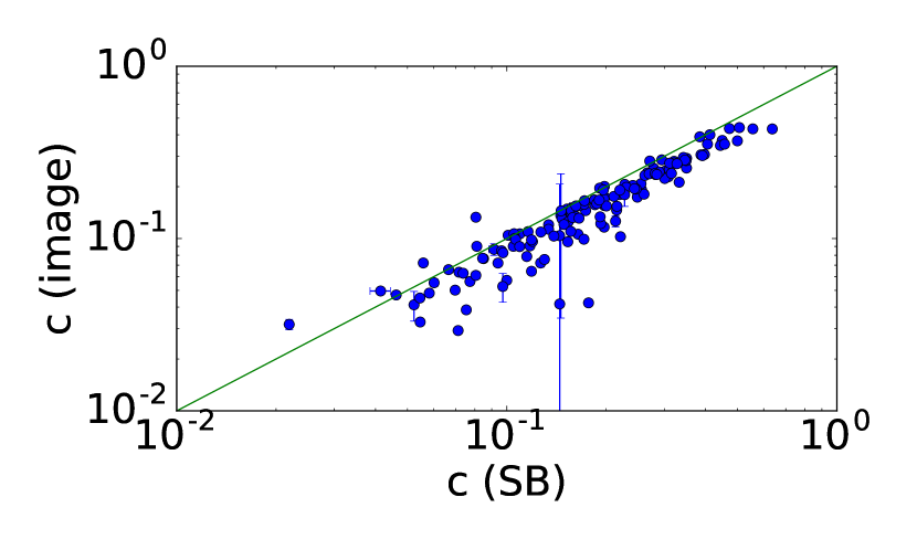
Figure B1: Comparison between the concentration values computed using the images and the SB profiles.

Table 4: Spearman and Pearson rank test correlation and probability for no correlation between the cluster global properties and the concentration parameter calculated using the XMM-Newton images.

	$R_{500}$
Relation	r	p-value	$\rho$	p-value
M500-c	0.03	0.77	0.01	0.91
LX-c	0.21	0.03	0.17	0.07
z-c	-0.17	0.06	-0.18	0.05

Appendix B Comparison between the concentration values obtained from the images and SB profiles

Due to the XMM-Newton PSF the surface brightness of a cluster look smoother than what it is in reality. In particular, the effect is bigger for the more distant objects because more photons originating in the center are spread out to much larger regions. As a consequence of that using the XMM-Newton images leads to systematic lower concentrations for the more distant objects than the low redshift clusters. On the other hand, by using the SB profiles might lead to some biases for the most disturbed systems because the clear substructures have to be removed to properly fit the profiles. Depending on the region where these substructures are the effect can be either reducing or increasing the concentration because of the lower number of counts within one of the two different circular apertures. In Fig. B1 we show the comparison between the concentration used in the paper (i.e. c(SB)) and the concentration calculated from the images. Indeed the correlation is good and in general SB profiles give a higher concentration because the PSF is taken into account. The correlation between the cluster global properties and the concentration computed with the images give qualitatively the same results as when the SB profiles are used for the concentration.

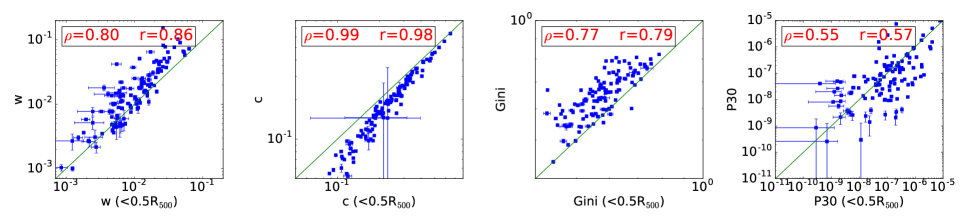
Figure C1: Comparison between the morphological parameters calculated within 0.5$R_{500}$ and $R_{500}$. Note that for this comparison both w values have been renormalized by $R_{500}$ (i.e. we divided by two the value of w(R$<$R₅₀₀)). The equality line is shown in green.

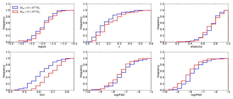
Figure C2: Comparison of the centroid shift (top-left), concentration (top-center), ellipticity (top-right), Gini coefficient (bottom-left), P30 (bottom-center), and P40 (bottom-right) values computed within 0.5$R_{500}$ and subdividing the sample by the total mass.

Figure C3: Comparison of the centroid shift (top-left), concentration (top-center), ellipticity (top-right), Gini coefficient (bottom-left), P30 (bottom-center), and P40 (bottom-right) values computed within 0.5$R_{500}$ and subdividing the sample by the total luminosity.

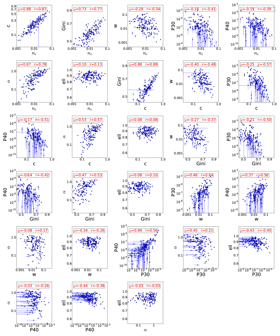
Figure C4: Parameters obtained within $0.5R_{500}$ plotted in the parameter-parameter planes. $\rho$ and r values indicate the Pearson and Spearman correlation coefficient (note that r is computed on ranks and so characterizes monotonic correlations, while $\rho$ is on true values and characterizes linear correlation). Some of the parameters show a clear and strong correlation while others are much more scattered.

Appendix C Cluster properties and morphology parameters at 0.5$R_{500}$

Clusters are continuously growing through accretion of smaller mass units. Substructures have been found to be relatively common in the outskirts of galaxy clusters (e.g. see for example the preliminary results of the XMM-Newton Cluster Outskirt Project, Eckert et al. 2017, Tchernin et al. 2016). As a consequence, the radius at which one computes the morphological parameters may assume a relevant role. Thus, if one limits the analyses to the innermost cluster regions (e.g. within 0.5$R_{500}$), one might miss some of the infalling structures and mark a cluster as relaxed instead of disturbed.

In Fig. C1 we compare w, c, g, and P30 calculated within 0.5R₅₀₀ and R₅₀₀ using only the clusters for which $R_{500}$ fits within the FOV. Indeed the concentration parameters show a very strong linear correlation (the Pearson rank test gives a correlation of 0.99) suggesting that the selection of clusters based on this parameter is not affected by using a different radius (i.e. the clusters with a high concentration at R₅₀₀ have also a high concentration at 0.5R₅₀₀). This is due to the continuous and smooth shape of the SB profiles and to the fact that they are derived after the removal of all the visible substructures. The other parameters show a similar linear correlation (0.80, 0.77, and 0.55 for w, g, and P30, respectively) but are more scattered. Centroid-shift and power ratios are more sensitive to the presence of substructures and so the choice of the radius used for the calculation has a larger impact. In fact, the centroid-shift measures the centroid variations in different aperture regions, so the presence of eventual substructures in the region 0.5-1R₅₀₀ can dramatically change the centroid position for half of the considered apertures (i.e. the 5 apertures with r$\leq n\times R_{500}$, with n=6-10). Similarly for the power ratios which are based on a 2D multipole expansion of the SB distribution (representing the mass distribution) and account for the azimuthal structures. The multipole moments are a measure for the substructures and depend on the distance to the origin of eventual substructures, as well as their angular dependence and since they are only sensitive to structures having a scale smaller than the considered aperture (see Buote & Tsai 1995 for more details about this last point) the choice of the radius at which P30 and P40 are calculated have impact on the results. Considering a smaller region (e.g. 0.5$R_{500}$ instead of $R_{500}$) leads to a smaller Gini coefficient because, as explained in Appendix A, all the low flux pixels that strongly contribute to move away the cumulative distribution from the even distribution are removed.

Despite the different parameter values at different scales the parameter-parameter relations calculated at 0.5$R_{500}$ are pretty similar to what obtained at $R_{500}$. In Fig. C4 we show the plots as Fig. 2, but obtained within 0.5$R_{500}$.

Similarly, when we compared the cluster properties with the morphological parameters computed within 0.5$R_{500}$ (see Fig. C2 and C3) we obtain qualitatively the same results as discussed in Sect. 4.4 and 5.3.

Appendix D Relaxed vs disturbed clusters

In Fig. D1 we show the distribution of the clusters visually classified as relaxed, “mix”, and disturbed for the combination of parameters that better perform in distinguishing the most relaxed and most disturbed systems (see Table 2).

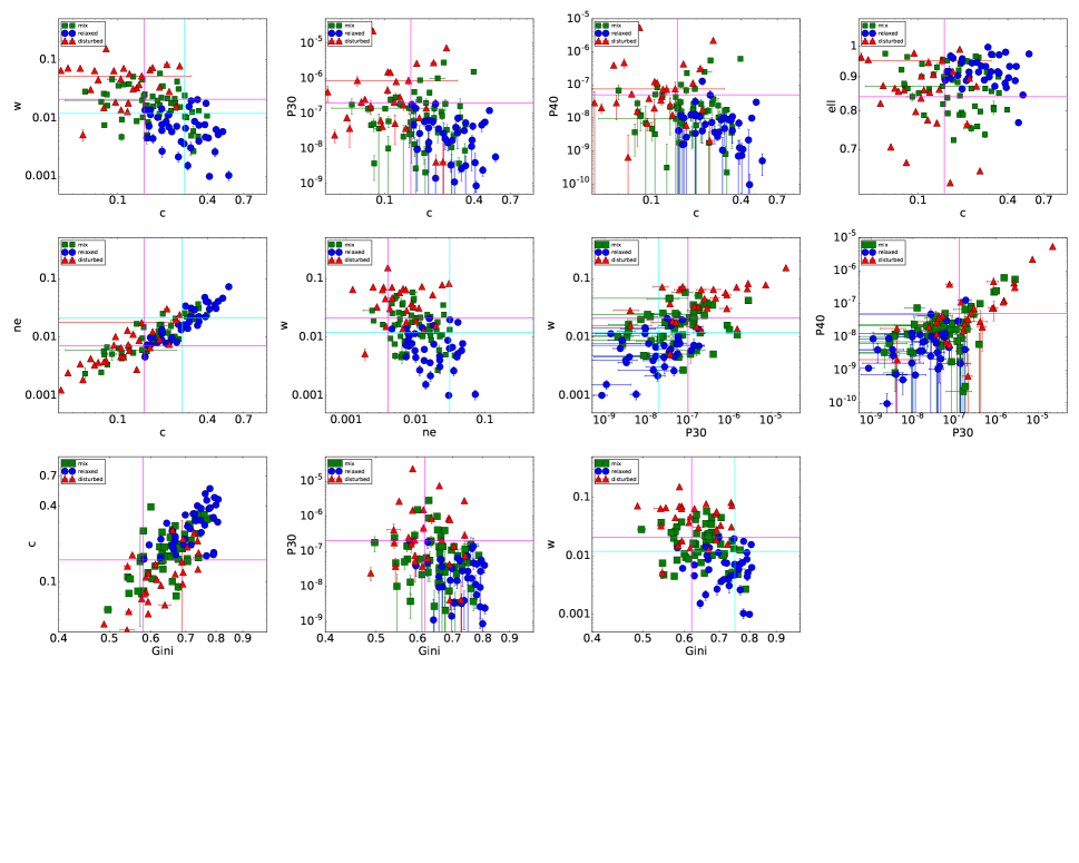
Figure D1: Distribution of the relaxed (blue), “mix” (green), and disturbed (red) clusters as a function of the different morphological parameters. The magenta and cyan lines represent the threshold values listed in Table 2 which were used to compute the completeness and the purity of the samples.

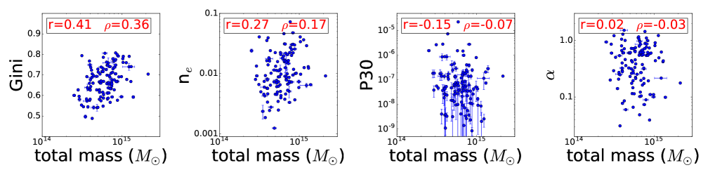
Figure F1: Correlations between the total mass and some of the morphological parameters computed within R₅₀₀. The correlation coefficient decreases from the left to the right.

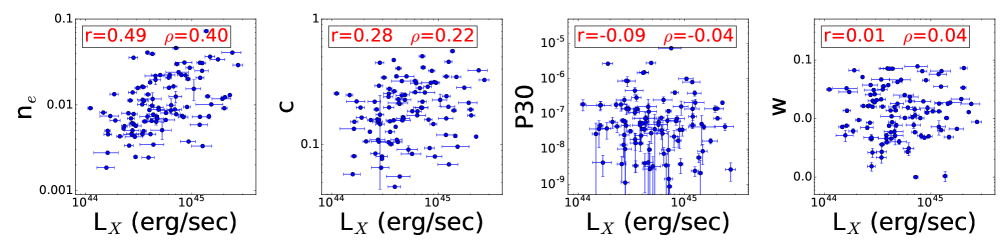
Figure F2: Correlations between the X-ray luminosity and some of the morphological parameters computed within R₅₀₀. The correlation coefficient decreases from the left to the right.

Table 5: Spearman and Pearson rank test correlation and probability for no correlation between the cluster global properties and the morphological parameters computed within 0.5$R_{500}$.

	$0.5R_{500}$
Relation	r	p-value	$\rho$	p-value
M500-c	0.09	0.27	0.03	0.70
M500-w	0.07	0.38	0.14	0.09
M500-$n_{e}$	0.28	$<$0.01	0.15	0.06
M500-Gini	0.10	0.24	0.05	0.58
M500-cusp	0.00	0.97	-0.05	0.59
M500-P30	0.10	0.25	-0.07	0.41
LX-c	0.28	$<0.01$	0.19	0.02
LX-w	-0.04	0.63	0.05	0.59
LX-$n_{e}$	0.50	$<$0.01	0.37	$<$0.01
LX-Gini	0.22	$<0.01$	0.09	0.28
LX-cusp	0.14	0.12	0.11	0.25
LX-P30	-0.05	0.58	-0.09	0.25

I1 I1: Pearson and Spearman rank test correlation and probability for no correlation between pairs of morphological parameters computed within $R_{500}$.

	$R_{500}$
Relation	$\rho$	p-value	r	p-value
$n_{e}-c$	0.87	$<$0.01	0.87	$<$0.01
$n_{e}-Gini$	0.66	$<$0.01	0.73	$<$0.01
$n_{e}-w$	-0.29	$<$0.01	-0.42	$<$0.01
$n_{e}-P30$	-0.06	0.48	-0.34	$<$0.01
$n_{e}-P40$	-0.06	0.50	-0.33	$<$0.01
$n_{e}-\alpha$	0.79	$<$0.01	0.81	$<$0.01
$n_{e}-ell$	0.02	0.85	0.05	0.60
$c-Gini$	0.71	$<$0.01	0.71	$<$0.01
$c-w$	-0.44	$<$0.01	-0.53	$<$0.01
$c-P30$	-0.11	0.24	-0.39	$<$0.01
$c-P40$	-0.10	0.30	-0.37	$<$0.01
$c-\alpha$	0.64	$<$0.01	0.60	$<$0.01
$c-ell$	0.08	0.41	0.08	0.39
$Gini-w$	-0.35	$<$0.01	-0.40	$<$0.01
$Gini-P30$	-0.14	0.13	-0.37	$<$0.01
$Gini-P40$	-0.14	0.12	-0.49	$<$0.01
$Gini-\alpha$	0.46	$<$0.01	0.46	$<$0.01
$Gini-ell$	0.18	0.05	0.20	0.03
$w-P30$	0.63	$<$0.01	0.53	$<$0.01
$w-P40$	0.61	$<$0.01	0.45	$<$0.01
$w-\alpha$	-0.22	0.02	-0.32	$<$0.01
$w-ell$	0.18	0.05	0.20	0.03
$P30-P40$	0.99	$<$0.01	0.56	$<$0.01
$P30-\alpha$	-0.04	0.68	-0.27	$<$0.01
$P30-ell$	-0.43	$<$0.01	-0.40	$<$0.01
$P40-\alpha$	-0.03	0.77	-0.26	$<$0.01
$P40-ell$	-0.44	$<$0.01	-0.38	$<$0.01
$\alpha-ell$	-0.03	0.71	-0.03	0.74

Appendix E Visual classification

The visual classification, apart from being subjective, might also depends on other criteria like, for example, the goodness of the images. We performed a few tests to ensure that our visual classification is robust.

First of all, we checked whether the same clusters are rated similarly when showed a second time to the six astronomers. This was done by showing multiple times the same images for 20 clusters, randomly chosen and displayed in a random order. All the 20 clusters have been classified in the same way (i.e. relaxed, “mix”, and disturbed) with an average dispersion around the mean of 0.25. In particular the most relaxed and most disturbed (i.e. the clusters with an average grade lower than 2 and greater than 3) show a smaller dispersion (0.13) than the “mix” objects (0.37).

Indeed, the number of counts is also an important parameter when classifying the clusters. Some clusters have very good data quality making easier to spot eventual surface brightness features. Furthermore, the image treatment can also play an important role because, for example, by progressively over-saturating the central regions of a cool core cluster may help to reveal more and more structures because the contrast in the outer regions starts to become more evident. To test whether these issues can bias the visual classification, a second image with reduced number of counts was produced and/or the color contrast changed for 40 galaxy clusters (again randomly selected). The new images were produced to have 10 to 30 thousand of source counts (corresponding, depending on the cluster, to 10-50$\%$ of the original total number of counts). Again, we found a very good agreement between the averaged grade obtained with the reduced and total number of counts. The dispersion around the mean was 0.14. Anyway, we note that for 62,5$\%$ of the objects the averaged grade is lower when the classification was done with reduced number of counts indicating as we said that a better data quality makes easier to identify possible substructures. Nonetheless, only two objects were classified differently from what done with the total number of counts. Moreover, given their morphological parameter values the qualitative results of the paper would not change because they would fall in the quadrants associated with the most relaxed clusters.

Appendix F Correlation plots between the cluster properties and the morphological parameters

Appendix G Cluster images

Although the classification is subjective, broadly speaking, objects with circular X-ray isophotes and without substructures are classified as relaxed, objects without substructures but not perfectly circular X-ray isophotes (e.g. sloshing) are classified as semi-relaxed, objects with substructures but still with a well formed cluster-core (e.g. A85) are classified as semi-disturbed, and double or complex objects with clear evidence of merging are classified as disturbed. See the cluster images in Fig. J1.

Appendix H Parameter values

All the parameter values used in this paper and calculated within R₅₀₀ are listed in Table H1.

Appendix I Parameter-parameter correlations

In Table I1 we list all the correlation coefficients and relative p-values for the plots showed in Fig. 2.

H1 H1: Morphological parameters for the 120 galaxy clusters with $R_{500}$ completely fitting withing the XMM-Newton FOV. The last column indicates if the cluster was visually classified as relaxed (R), mix (M), or disturbed (D).

Planck	alternative	R500	$n_{e}$	$cusp$	$c$	$w$	$Gini$	$P30$	$P40$	$ell$	Dynamical
name	name	kpc	$\times 10^{-2}$			$\times 10^{-2}$		$\times 10^{-7}$	$\times 10^{-8}$		State
G000.44-41.83	A3739	1114	0.73 $\pm$ 0.05	0.33 $\pm$ 0.01	0.16 $\pm$ 0.01	0.46 $\pm$ 0.06	0.63 $\pm$ 0.01	0.48 $\pm$ 0.29	1.19 $\pm$ 0.93	0.92 $\pm$ 0.01	R
G002.74-56.18	RXCJ2218.6-3853	1106	1.01 $\pm$ 0.01	0.36 $\pm$ 0.01	0.24 $\pm$ 0.01	2.13 $\pm$ 0.04	0.70 $\pm$ 0.01	1.08 $\pm$ 0.16	1.66 $\pm$ 0.41	0.81 $\pm$ 0.01	M
G003.90-59.41	A3888	1270	0.99 $\pm$ 0.20	0.55 $\pm$ 0.01	0.18 $\pm$ 0.01	1.99 $\pm$ 0.03	0.69 $\pm$ 0.01	0.07 $\pm$ 0.04	1.21 $\pm$ 0.29	0.88 $\pm$ 0.01	M
G006.70-35.54	A3695	1065	0.57 $\pm$ 0.01	0.66 $\pm$ 0.01	0.08 $\pm$ 0.01	2.61 $\pm$ 0.05	0.58 $\pm$ 0.01	1.39 $\pm$ 0.29	2.75 $\pm$ 0.80	0.88 $\pm$ 0.01	M
G006.78+30.46	A2163	1817	0.92 $\pm$ 0.01	0.18 $\pm$ 0.01	0.19 $\pm$ 0.01	3.36 $\pm$ 0.01	0.70 $\pm$ 0.01	1.42 $\pm$ 0.04	11.40 $\pm$ 0.27	0.99 $\pm$ 0.01	D
G008.44-56.35	A3854	1061	1.64 $\pm$ 0.01	0.80 $\pm$ 0.01	0.25 $\pm$ 0.01	0.22 $\pm$ 0.04	0.66 $\pm$ 0.01	0.19 $\pm$ 0.10	0.73 $\pm$ 0.32	0.92 $\pm$ 0.01	R
G008.93-81.23	A2744	1360	0.59 $\pm$ 0.01	0.11 $\pm$ 0.01	0.12 $\pm$ 0.01	5.74 $\pm$ 0.03	0.69 $\pm$ 0.01	8.05 $\pm$ 0.21	7.37 $\pm$ 0.36	0.85 $\pm$ 0.01	D
G021.09+33.25	A2204	1323	7.25 $\pm$ 0.03	1.44 $\pm$ 0.01	0.56 $\pm$ 0.01	0.10 $\pm$ 0.02	0.78 $\pm$ 0.01	0.06 $\pm$ 0.02	0.05 $\pm$ 0.03	0.97 $\pm$ 0.01	R
G036.72+14.92		1241	1.96 $\pm$ 0.24	1.12 $\pm$ 0.01	0.25 $\pm$ 0.01	1.58 $\pm$ 0.05	0.73 $\pm$ 0.01	0.04 $\pm$ 0.10	0.20 $\pm$ 0.53	0.87 $\pm$ 0.01	D
G039.85-39.98	A2345	1077	0.24 $\pm$ 0.01	0.09 $\pm$ 0.01	0.05 $\pm$ 0.01	7.19 $\pm$ 0.05	0.49 $\pm$ 0.01	0.24 $\pm$ 0.10	2.04 $\pm$ 0.68	0.95 $\pm$ 0.01	D
G042.82+56.61	A2065	1189	1.13 $\pm$ 0.01	0.72 $\pm$ 0.01	0.19 $\pm$ 0.01	1.66 $\pm$ 0.03	0.62 $\pm$ 0.01	0.65 $\pm$ 0.09	1.77 $\pm$ 0.35	0.84 $\pm$ 0.01	M
G046.08+27.18	RXCJ1731+22	1148	0.38 $\pm$ 0.01	0.05 $\pm$ 0.01	0.08 $\pm$ 0.01	1.51 $\pm$ 0.18	0.58 $\pm$ 0.01	1.62 $\pm$ 0.70	1.59 $\pm$ 1.45	0.86 $\pm$ 0.01	D
G046.50-49.43	A2420	1194	0.70 $\pm$ 0.01	0.44 $\pm$ 0.01	0.16 $\pm$ 0.01	0.85 $\pm$ 0.03	0.58 $\pm$ 0.01	0.13 $\pm$ 0.07	1.58 $\pm$ 0.57	0.91 $\pm$ 0.01	M
G049.20+30.86	RXJ1720.1+2638	1241	4.61 $\pm$ 0.01	1.16 $\pm$ 0.01	0.51 $\pm$ 0.01	0.58 $\pm$ 0.04	0.76 $\pm$ 0.01	1.20 $\pm$ 0.15	2.99 $\pm$ 0.61	0.84 $\pm$ 0.01	R
G049.33+44.38	A2175	1049	0.46 $\pm$ 0.01	0.21 $\pm$ 0.01	0.15 $\pm$ 0.01	1.36 $\pm$ 0.10	0.58 $\pm$ 0.01	1.78 $\pm$ 0.47	0.41 $\pm$ 0.60	0.89 $\pm$ 0.01	R
G049.66-49.50	A2426	1090	1.40 $\pm$ 0.01	0.60 $\pm$ 0.01	0.29 $\pm$ 0.01	0.15 $\pm$ 0.03	0.64 $\pm$ 0.01	0.01 $\pm$ 0.03	0.88 $\pm$ 0.48	1.00 $\pm$ 0.01	R
G053.52+59.54	A2034	1189	0.50 $\pm$ 0.01	0.12 $\pm$ 0.01	0.15 $\pm$ 0.01	1.60 $\pm$ 0.07	0.70 $\pm$ 0.01	1.36 $\pm$ 0.24	0.18 $\pm$ 0.22	0.90 $\pm$ 0.01	M
G055.60+31.86	A2261	1234	3.10 $\pm$ 0.01	0.95 $\pm$ 0.01	0.35 $\pm$ 0.01	1.33 $\pm$ 0.03	0.75 $\pm$ 0.01	0.48 $\pm$ 0.08	0.54 $\pm$ 0.16	0.85 $\pm$ 0.01	M
G055.97-34.88	A2355	1110	0.28 $\pm$ 0.01	0.06 $\pm$ 0.01	0.13 $\pm$ 0.01	3.29 $\pm$ 0.09	0.54 $\pm$ 0.01	1.75 $\pm$ 0.54	2.49 $\pm$ 1.63	0.77 $\pm$ 0.01	D
G056.81+36.31	A2244	1098	1.83 $\pm$ 0.01	0.60 $\pm$ 0.01	0.35 $\pm$ 0.01	0.75 $\pm$ 0.02	0.72 $\pm$ 0.01	0.54 $\pm$ 0.06	1.10 $\pm$ 0.18	0.91 $\pm$ 0.01	R
G056.96-55.07		1255	1.01 $\pm$ 0.01	0.60 $\pm$ 0.01	0.10 $\pm$ 0.01	1.87 $\pm$ 0.04	0.69 $\pm$ 0.01	0.42 $\pm$ 0.07	3.87 $\pm$ 0.41	0.80 $\pm$ 0.01	D
G057.26-45.35	RXCJ2211.7-0350	1334	4.07 $\pm$ 0.03	0.81 $\pm$ 0.01	0.39 $\pm$ 0.01	1.78 $\pm$ 0.04	0.78 $\pm$ 0.01	0.43 $\pm$ 0.10	0.13 $\pm$ 0.09	0.87 $\pm$ 0.01	R
G058.28+18.59	RXCJ1825.3+3026	1028	0.50 $\pm$ 0.01	0.50 $\pm$ 0.01	0.08 $\pm$ 0.01	0.76 $\pm$ 0.01	0.55 $\pm$ 0.01	0.46 $\pm$ 0.07	1.48 $\pm$ 0.31	0.87 $\pm$ 0.01	M
G062.42-46.41	A2440	998	0.66 $\pm$ 0.01	0.29 $\pm$ 0.01	0.16 $\pm$ 0.01	6.69 $\pm$ 0.06	0.55 $\pm$ 0.01	26.80 $\pm$ 1.03	43.00 $\pm$ 2.94	0.62 $\pm$ 0.01	D
G067.23+67.46	A1914	1334	2.00 $\pm$ 0.01	0.54 $\pm$ 0.01	0.32 $\pm$ 0.01	1.26 $\pm$ 0.01	0.77 $\pm$ 0.01	0.04 $\pm$ 0.02	0.08 $\pm$ 0.06	0.97 $\pm$ 0.01	M
G071.61+29.79		1039	0.19 $\pm$ 0.01	0.03 $\pm$ 0.01	0.06 $\pm$ 0.01	0.52 $\pm$ 0.11	0.54 $\pm$ 0.01	0.37 $\pm$ 0.27	2.88 $\pm$ 2.02	0.87 $\pm$ 0.01	D
G072.63+41.46	A2219	1475	1.26 $\pm$ 0.01	0.49 $\pm$ 0.01	0.19 $\pm$ 0.01	1.02 $\pm$ 0.05	0.68 $\pm$ 0.01	0.02 $\pm$ 0.03	0.34 $\pm$ 0.22	0.92 $\pm$ 0.01	M
G072.80-18.72		1249	1.64 $\pm$ 0.01	1.06 $\pm$ 0.01	0.20 $\pm$ 0.01	2.23 $\pm$ 0.04	0.66 $\pm$ 0.01	0.12 $\pm$ 0.06	7.53 $\pm$ 1.19	0.80 $\pm$ 0.01	M
G073.96-27.82	A2390	1492	3.65 $\pm$ 0.01	1.22 $\pm$ 0.01	0.35 $\pm$ 0.01	0.48 $\pm$ 0.04	0.76 $\pm$ 0.01	0.09 $\pm$ 0.05	0.36 $\pm$ 0.24	0.90 $\pm$ 0.01	M
G080.38-33.20	A2443	1053	0.74 $\pm$ 0.01	0.27 $\pm$ 0.01	0.22 $\pm$ 0.01	2.85 $\pm$ 0.02	0.69 $\pm$ 0.01	0.04 $\pm$ 0.02	1.79 $\pm$ 0.25	0.90 $\pm$ 0.01	D
G080.99-50.90	A2552	1208	1.54 $\pm$ 0.42	0.27 $\pm$ 0.01	0.23 $\pm$ 0.03	1.33 $\pm$ 0.09	0.65 $\pm$ 0.01	10.01 $\pm$ 1.13	24.90 $\pm$ 3.74	0.75 $\pm$ 0.01	M
G083.28-31.03	RXCJ2228.6+2036	1242	1.18 $\pm$ 0.03	0.19 $\pm$ 0.01	0.22 $\pm$ 0.01	2.16 $\pm$ 0.09	0.67 $\pm$ 0.01	1.40 $\pm$ 0.30	2.67 $\pm$ 1.01	0.89 $\pm$ 0.01	M
G085.99+26.71	A2302	1011	0.24 $\pm$ 0.06	0.14 $\pm$ 0.01	0.06 $\pm$ 0.01	2.83 $\pm$ 0.14	0.50 $\pm$ 0.01	1.78 $\pm$ 0.83	6.76 $\pm$ 3.28	0.97 $\pm$ 0.01	M
G086.45+15.29		1270	2.23 $\pm$ 0.06	0.72 $\pm$ 0.01	0.29 $\pm$ 0.01	1.02 $\pm$ 0.06	0.71 $\pm$ 0.01	0.23 $\pm$ 0.12	1.05 $\pm$ 0.56	0.92 $\pm$ 0.01	M
G092.73+73.46	A1763	1271	0.74 $\pm$ 0.01	0.17 $\pm$ 0.01	0.16 $\pm$ 0.01	0.51 $\pm$ 0.06	0.66 $\pm$ 0.01	4.06 $\pm$ 0.52	10.20 $\pm$ 1.83	0.79 $\pm$ 0.01	M
G093.91+34.90	A2255	1211	0.25 $\pm$ 0.01	0.07 $\pm$ 0.01	0.08 $\pm$ 0.01	1.90 $\pm$ 0.06	0.67 $\pm$ 0.01	1.35 $\pm$ 0.30	0.37 $\pm$ 0.30	0.92 $\pm$ 0.01	M
G096.87+24.21		1074	0.12 $\pm$ 0.01	0.01 $\pm$ 0.01	0.04 $\pm$ 0.01	6.51 $\pm$ 0.22	0.54 $\pm$ 0.02	4.10 $\pm$ 1.99	2.88 $\pm$ 3.42	0.96 $\pm$ 0.01	D
G097.73+38.11	A2218	1179	0.73 $\pm$ 0.01	0.27 $\pm$ 0.01	0.17 $\pm$ 0.01	1.38 $\pm$ 0.05	0.67 $\pm$ 0.01	0.10 $\pm$ 0.07	1.00 $\pm$ 0.42	0.90 $\pm$ 0.01	R
G098.95+24.86	A2312	995	0.92 $\pm$ 0.01	0.60 $\pm$ 0.01	0.26 $\pm$ 0.01	3.15 $\pm$ 0.09	0.58 $\pm$ 0.01	1.87 $\pm$ 0.66	2.67 $\pm$ 1.44	0.96 $\pm$ 0.01	M
G106.73-83.22	A2813	1132	0.89 $\pm$ 0.01	0.11 $\pm$ 0.01	0.20 $\pm$ 0.01	0.77 $\pm$ 0.10	0.72 $\pm$ 0.01	0.64 $\pm$ 0.28	3.12 $\pm$ 1.19	0.95 $\pm$ 0.01	R
G107.11+65.31	A1758	1186	0.65 $\pm$ 0.01	0.33 $\pm$ 0.01	0.11 $\pm$ 0.01	1.37 $\pm$ 0.05	0.62 $\pm$ 0.01	15.30 $\pm$ 0.87	12.60 $\pm$ 1.56	0.90 $\pm$ 0.01	D
G113.82+44.35	A1895	1139	0.46 $\pm$ 0.03	0.17 $\pm$ 0.01	0.10 $\pm$ 0.01	4.65 $\pm$ 0.14	0.62 $\pm$ 0.01	4.60 $\pm$ 1.15	2.00 $\pm$ 1.63	0.84 $\pm$ 0.01	D
G124.21-36.48	A115N	1072	2.41 $\pm$ 0.01	1.00 $\pm$ 0.01	0.26 $\pm$ 0.01	7.80 $\pm$ 0.04	0.66 $\pm$ 0.01	74.10 $\pm$ 1.40	222.00 $\pm$ 5.14	0.65 $\pm$ 0.01	D
G125.70+53.85	A1576	1197	1.25 $\pm$ 0.20	0.60 $\pm$ 0.01	0.20 $\pm$ 0.01	1.44 $\pm$ 0.15	0.66 $\pm$ 0.01	0.09 $\pm$ 0.22	1.29 $\pm$ 1.81	0.95 $\pm$ 0.01	R
G139.19+56.35	A1351	1228	0.51 $\pm$ 0.11	0.31 $\pm$ 0.01	0.09 $\pm$ 0.01	4.60 $\pm$ 0.20	0.68 $\pm$ 0.01	0.37 $\pm$ 0.60	0.71 $\pm$ 1.60	0.84 $\pm$ 0.01	M
G149.73+34.69	A0665	1353	0.95 $\pm$ 0.01	0.56 $\pm$ 0.01	0.15 $\pm$ 0.01	4.52 $\pm$ 0.09	0.71 $\pm$ 0.01	0.35 $\pm$ 0.25	4.27 $\pm$ 1.76	0.95 $\pm$ 0.01	M
G157.43+30.33		1125	1.68 $\pm$ 0.01	0.98 $\pm$ 0.01	0.13 $\pm$ 0.01	0.88 $\pm$ 0.07	0.61 $\pm$ 0.01	0.22 $\pm$ 0.23	2.14 $\pm$ 1.83	0.93 $\pm$ 0.01	M
G159.85-73.47	A0209	1245	0.81 $\pm$ 0.04	0.20 $\pm$ 0.01	0.18 $\pm$ 0.01	1.02 $\pm$ 0.07	0.66 $\pm$ 0.01	0.58 $\pm$ 0.15	1.26 $\pm$ 0.47	0.90 $\pm$ 0.01	R
G164.18-38.89	A0399	1119	0.64 $\pm$ 0.01	0.46 $\pm$ 0.01	0.10 $\pm$ 0.01	3.56 $\pm$ 0.04	0.66 $\pm$ 0.01	1.36 $\pm$ 0.18	0.47 $\pm$ 0.27	0.85 $\pm$ 0.01	M
G166.13+43.39	A0773	1250	0.78 $\pm$ 0.01	0.10 $\pm$ 0.01	0.22 $\pm$ 0.01	1.14 $\pm$ 0.06	0.70 $\pm$ 0.01	0.01 $\pm$ 0.02	0.41 $\pm$ 0.24	0.92 $\pm$ 0.01	R
G167.65+17.64		1299	0.69 $\pm$ 0.01	0.21 $\pm$ 0.01	0.16 $\pm$ 0.01	0.77 $\pm$ 0.07	0.65 $\pm$ 0.01	0.03 $\pm$ 0.05	0.63 $\pm$ 0.40	0.90 $\pm$ 0.01	M
G171.94-40.65		1408	0.98 $\pm$ 0.01	0.44 $\pm$ 0.01	0.17 $\pm$ 0.01	1.14 $\pm$ 0.07	0.79 $\pm$ 0.01	0.09 $\pm$ 0.09	0.16 $\pm$ 0.25	0.97 $\pm$ 0.01	R
G180.24+21.04		1358	1.30 $\pm$ 0.04	0.42 $\pm$ 0.01	0.12 $\pm$ 0.01	1.29 $\pm$ 0.05	0.67 $\pm$ 0.01	2.09 $\pm$ 0.24	3.46 $\pm$ 0.60	0.78 $\pm$ 0.01	D
G182.44-28.29	A0478	1415	3.00 $\pm$ 0.02	0.74 $\pm$ 0.01	0.41 $\pm$ 0.01	0.10 $\pm$ 0.01	0.80 $\pm$ 0.01	0.01 $\pm$ 0.01	0.11 $\pm$ 0.02	0.93 $\pm$ 0.01	R
G182.63+55.82	A0963	1126	2.23 $\pm$ 0.01	0.60 $\pm$ 0.01	0.35 $\pm$ 0.01	0.40 $\pm$ 0.04	0.73 $\pm$ 0.01	0.03 $\pm$ 0.03	0.41 $\pm$ 0.24	0.97 $\pm$ 0.01	R
G186.39+37.25	A0697	1280	0.73 $\pm$ 0.01	0.09 $\pm$ 0.01	0.16 $\pm$ 0.01	0.72 $\pm$ 0.20	0.77 $\pm$ 0.02	1.39 $\pm$ 1.01	0.16 $\pm$ 1.07	0.92 $\pm$ 0.02	R
G195.62+44.05	A0781	1105	0.34 $\pm$ 0.01	0.15 $\pm$ 0.01	0.06 $\pm$ 0.01	7.11 $\pm$ 0.05	0.59 $\pm$ 0.01	0.75 $\pm$ 0.14	39.50 $\pm$ 2.17	0.82 $\pm$ 0.01	D
G195.77-24.30	A0520	1314	0.72 $\pm$ 0.01	0.76 $\pm$ 0.01	0.09 $\pm$ 0.01	6.46 $\pm$ 0.05	0.63 $\pm$ 0.01	0.63 $\pm$ 0.15	0.69 $\pm$ 0.29	0.98 $\pm$ 0.01	D
G218.85+35.50	A0750	1050	0.93 $\pm$ 0.01	0.25 $\pm$ 0.01	0.25 $\pm$ 0.01	4.21 $\pm$ 0.09	0.63 $\pm$ 0.01	28.20 $\pm$ 1.94	54.90 $\pm$ 4.61	0.76 $\pm$ 0.01	M
G225.92-19.99		1187	3.03 $\pm$ 0.02	0.87 $\pm$ 0.01	0.21 $\pm$ 0.01	8.25 $\pm$ 0.12	0.74 $\pm$ 0.01	27.90 $\pm$ 1.65	31.50 $\pm$ 4.45	0.76 $\pm$ 0.01	D

H1 H1: continued from previous page

Planck	alternative	R500	$n_{e}$	$cusp$	$c$	$w$	$Gini$	$P30$	$P40$	$ell$	Dynamical
name	name	kpc	$\times 10^{-2}$			$\times 10^{-2}$		$\times 10^{-7}$	$\times 10^{-8}$		State
G226.17-21.91	A0550	1087	0.57 $\pm$ 0.02	0.28 $\pm$ 0.01	0.16 $\pm$ 0.01	1.64 $\pm$ 0.04	0.63 $\pm$ 0.01	0.44 $\pm$ 0.14	2.99 $\pm$ 0.88	0.84 $\pm$ 0.01	M
G226.24+76.76	A1413	1215	2.08 $\pm$ 0.01	0.74 $\pm$ 0.01	0.32 $\pm$ 0.01	0.27 $\pm$ 0.01	0.79 $\pm$ 0.01	0.77 $\pm$ 0.02	1.77 $\pm$ 0.07	0.80 $\pm$ 0.01	M
G228.15+75.19		1239	0.73 $\pm$ 0.05	0.10 $\pm$ 0.01	0.12 $\pm$ 0.01	1.80 $\pm$ 0.15	0.59 $\pm$ 0.01	0.52 $\pm$ 0.39	4.41 $\pm$ 1.97	0.95 $\pm$ 0.01	D
G228.49+53.12		1061	3.55 $\pm$ 0.01	1.05 $\pm$ 0.01	0.45 $\pm$ 0.01	0.26 $\pm$ 0.05	0.77 $\pm$ 0.01	0.46 $\pm$ 0.16	0.21 $\pm$ 0.24	0.89 $\pm$ 0.01	R
G229.21-17.24		1136	0.45 $\pm$ 0.01	0.23 $\pm$ 0.01	0.11 $\pm$ 0.01	3.74 $\pm$ 0.10	0.54 $\pm$ 0.01	2.48 $\pm$ 0.56	8.34 $\pm$ 2.53	0.79 $\pm$ 0.01	M
G229.94+15.29	A0644	1289	1.57 $\pm$ 0.01	0.55 $\pm$ 0.01	0.34 $\pm$ 0.01	2.06 $\pm$ 0.01	0.70 $\pm$ 0.01	0.32 $\pm$ 0.04	0.83 $\pm$ 0.13	0.92 $\pm$ 0.01	R
G236.95-26.67	A3364	1206	0.77 $\pm$ 0.01	0.31 $\pm$ 0.01	0.21 $\pm$ 0.01	0.87 $\pm$ 0.04	0.67 $\pm$ 0.01	0.58 $\pm$ 0.14	1.09 $\pm$ 0.36	0.89 $\pm$ 0.01	R
G241.74-30.88	RXCJ0532.9-3701	1159	2.23 $\pm$ 0.02	0.63 $\pm$ 0.01	0.31 $\pm$ 0.01	0.31 $\pm$ 0.08	0.73 $\pm$ 0.01	0.28 $\pm$ 0.18	1.04 $\pm$ 0.71	0.92 $\pm$ 0.01	R
G241.77-24.00	A3378	1070	3.94 $\pm$ 0.01	1.29 $\pm$ 0.01	0.41 $\pm$ 0.01	0.46 $\pm$ 0.02	0.74 $\pm$ 0.01	0.04 $\pm$ 0.03	0.07 $\pm$ 0.10	0.90 $\pm$ 0.01	R
G241.97+14.85	A3411	1254	0.46 $\pm$ 0.01	0.12 $\pm$ 0.01	0.11 $\pm$ 0.01	7.11 $\pm$ 0.03	0.59 $\pm$ 0.01	14.80 $\pm$ 0.37	11.50 $\pm$ 0.74	0.86 $\pm$ 0.01	D
G244.34-32.13	RXCJ0528.9-3927	1229	2.07 $\pm$ 0.06	0.67 $\pm$ 0.01	0.24 $\pm$ 0.01	1.80 $\pm$ 0.08	0.74 $\pm$ 0.01	0.84 $\pm$ 0.19	0.18 $\pm$ 0.21	0.97 $\pm$ 0.01	M
G244.69+32.49	A0868	1069	0.46 $\pm$ 0.01	0.08 $\pm$ 0.01	0.15 $\pm$ 0.01	2.54 $\pm$ 0.15	0.68 $\pm$ 0.01	0.25 $\pm$ 0.21	2.21 $\pm$ 1.42	0.90 $\pm$ 0.01	M
G247.17-23.32	ABELLS0579	1031	0.60 $\pm$ 0.03	0.25 $\pm$ 0.01	0.15 $\pm$ 0.10	2.01 $\pm$ 0.09	0.57 $\pm$ 0.01	1.41 $\pm$ 0.47	0.94 $\pm$ 0.96	0.87 $\pm$ 0.01	M
G249.87-39.86	A3292	948	0.80 $\pm$ 0.01	0.20 $\pm$ 0.01	0.22 $\pm$ 0.01	0.70 $\pm$ 0.05	0.63 $\pm$ 0.01	1.85 $\pm$ 0.65	12.90 $\pm$ 3.02	0.90 $\pm$ 0.01	R
G250.90-36.25	A3322	1155	0.88 $\pm$ 0.01	0.19 $\pm$ 0.01	0.23 $\pm$ 0.01	1.79 $\pm$ 0.06	0.66 $\pm$ 0.01	0.28 $\pm$ 0.14	1.50 $\pm$ 0.73	0.86 $\pm$ 0.01	M
G252.96-56.05	A3112	1006	4.08 $\pm$ 0.01	1.21 $\pm$ 0.01	0.47 $\pm$ 0.01	0.52 $\pm$ 0.01	0.79 $\pm$ 0.01	0.56 $\pm$ 0.03	0.99 $\pm$ 0.07	0.77 $\pm$ 0.01	R
G253.47-33.72	A3343	1118	1.15 $\pm$ 0.01	0.60 $\pm$ 0.01	0.20 $\pm$ 0.01	0.27 $\pm$ 0.06	0.69 $\pm$ 0.01	0.15 $\pm$ 0.13	1.16 $\pm$ 0.84	0.96 $\pm$ 0.01	R
G256.45-65.71	A3017	1143	1.58 $\pm$ 0.02	0.42 $\pm$ 0.01	0.26 $\pm$ 0.01	1.54 $\pm$ 0.05	0.66 $\pm$ 0.01	0.34 $\pm$ 0.15	3.69 $\pm$ 0.92	0.80 $\pm$ 0.01	M
G257.34-22.18	A3399	1168	1.11 $\pm$ 0.02	0.72 $\pm$ 0.01	0.13 $\pm$ 0.01	3.14 $\pm$ 0.14	0.74 $\pm$ 0.01	2.90 $\pm$ 0.61	7.36 $\pm$ 2.45	0.91 $\pm$ 0.01	D
G260.03-63.44	RXCJ0232.2-4420	1196	3.12 $\pm$ 0.01	0.79 $\pm$ 0.01	0.31 $\pm$ 0.01	1.97 $\pm$ 0.04	0.75 $\pm$ 0.01	0.73 $\pm$ 0.17	0.48 $\pm$ 0.33	0.97 $\pm$ 0.01	R
G262.25-35.36	RXCJ0516.7-5430	1247	0.33 $\pm$ 0.01	0.07 $\pm$ 0.01	0.07 $\pm$ 0.01	6.47 $\pm$ 0.13	0.59 $\pm$ 0.01	2.09 $\pm$ 0.54	0.07 $\pm$ 0.24	0.86 $\pm$ 0.01	D
G262.71-40.91		1123	1.80 $\pm$ 0.02	0.25 $\pm$ 0.01	0.30 $\pm$ 0.01	1.56 $\pm$ 0.06	0.81 $\pm$ 0.01	0.40 $\pm$ 0.16	0.11 $\pm$ 0.15	0.90 $\pm$ 0.01	R
G263.16-23.41	AbellS0592	1294	2.71 $\pm$ 0.01	0.89 $\pm$ 0.01	0.31 $\pm$ 0.01	0.50 $\pm$ 0.03	0.73 $\pm$ 0.01	0.35 $\pm$ 0.12	1.69 $\pm$ 0.44	0.86 $\pm$ 0.01	M
G263.66-22.53	A3404	1297	1.65 $\pm$ 0.02	0.56 $\pm$ 0.01	0.28 $\pm$ 0.01	1.05 $\pm$ 0.04	0.71 $\pm$ 0.01	0.03 $\pm$ 0.03	1.03 $\pm$ 0.44	0.86 $\pm$ 0.01	M
G266.03-21.25		1499	1.23 $\pm$ 0.01	0.44 $\pm$ 0.01	0.17 $\pm$ 0.01	7.30 $\pm$ 0.03	0.74 $\pm$ 0.01	0.75 $\pm$ 0.09	0.60 $\pm$ 0.17	0.92 $\pm$ 0.01	D
G269.31-49.87	A3126	1098	0.81 $\pm$ 0.01	0.32 $\pm$ 0.01	0.25 $\pm$ 0.01	0.72 $\pm$ 0.05	0.75 $\pm$ 0.01	0.27 $\pm$ 0.28	4.89 $\pm$ 1.97	0.95 $\pm$ 0.01	R
G271.19-30.96		1250	4.76 $\pm$ 0.08	0.99 $\pm$ 0.01	0.38 $\pm$ 0.01	0.77 $\pm$ 0.05	0.78 $\pm$ 0.01	0.11 $\pm$ 0.09	0.07 $\pm$ 0.14	0.88 $\pm$ 0.01	R
G271.50-56.55	S0295	1200	0.90 $\pm$ 0.14	0.10 $\pm$ 0.01	0.19 $\pm$ 0.01	5.80 $\pm$ 0.09	0.66 $\pm$ 0.01	0.86 $\pm$ 0.46	2.60 $\pm$ 1.31	0.94 $\pm$ 0.01	M
G272.10-40.15	A3266	1316	0.87 $\pm$ 0.01	0.61 $\pm$ 0.01	0.14 $\pm$ 0.01	3.73 $\pm$ 0.01	0.61 $\pm$ 0.01	0.37 $\pm$ 0.03	1.23 $\pm$ 0.12	0.86 $\pm$ 0.01	D
G277.75-51.73		1238	0.37 $\pm$ 0.01	0.04 $\pm$ 0.01	0.07 $\pm$ 0.01	4.52 $\pm$ 0.07	0.58 $\pm$ 0.01	2.50 $\pm$ 0.38	5.28 $\pm$ 0.96	0.86 $\pm$ 0.01	D
G278.60+39.17	A1300	1268	2.50 $\pm$ 0.01	1.10 $\pm$ 0.01	0.20 $\pm$ 0.01	3.51 $\pm$ 0.08	0.68 $\pm$ 0.01	3.90 $\pm$ 0.68	0.60 $\pm$ 0.69	0.79 $\pm$ 0.01	M
G280.19+47.81	A1391	1201	0.51 $\pm$ 0.01	0.45 $\pm$ 0.01	0.11 $\pm$ 0.01	0.47 $\pm$ 0.06	0.55 $\pm$ 0.01	0.10 $\pm$ 0.12	0.32 $\pm$ 0.59	0.90 $\pm$ 0.01	M
G282.49+65.17	ZwCl1215	1212	0.61 $\pm$ 0.02	0.29 $\pm$ 0.01	0.16 $\pm$ 0.01	0.45 $\pm$ 0.02	0.57 $\pm$ 0.01	0.60 $\pm$ 0.10	1.05 $\pm$ 0.26	0.95 $\pm$ 0.01	M
G283.16-22.93		1137	1.62 $\pm$ 0.01	0.63 $\pm$ 0.01	0.19 $\pm$ 0.01	1.18 $\pm$ 0.11	0.64 $\pm$ 0.01	1.98 $\pm$ 0.65	1.73 $\pm$ 1.60	0.79 $\pm$ 0.01	M
G284.46+52.43	RXJ1206.2-0848	1308	3.39 $\pm$ 0.01	0.91 $\pm$ 0.01	0.28 $\pm$ 0.01	0.67 $\pm$ 0.02	0.76 $\pm$ 0.01	0.17 $\pm$ 0.03	0.37 $\pm$ 0.09	0.93 $\pm$ 0.01	R
G284.99-23.70		1266	2.56 $\pm$ 0.02	0.58 $\pm$ 0.01	0.28 $\pm$ 0.01	2.42 $\pm$ 0.11	0.67 $\pm$ 0.01	0.11 $\pm$ 0.20	2.37 $\pm$ 1.53	0.74 $\pm$ 0.01	M
G285.63-17.24		1007	1.76 $\pm$ 0.10	1.51 $\pm$ 0.01	0.14 $\pm$ 0.17	5.25 $\pm$ 0.16	0.69 $\pm$ 0.01	8.66 $\pm$ 2.24	7.55 $\pm$ 4.53	0.95 $\pm$ 0.01	D
G286.58-31.25		1141	0.61 $\pm$ 0.01	0.26 $\pm$ 0.01	0.15 $\pm$ 0.01	1.03 $\pm$ 0.06	0.63 $\pm$ 0.01	0.25 $\pm$ 0.12	2.33 $\pm$ 0.79	0.82 $\pm$ 0.01	M
G286.99+32.91		1476	0.66 $\pm$ 0.01	0.10 $\pm$ 0.01	0.12 $\pm$ 0.01	3.82 $\pm$ 0.11	0.59 $\pm$ 0.01	2.87 $\pm$ 0.92	4.82 $\pm$ 1.78	0.86 $\pm$ 0.01	M
G288.61-37.65	A3186	1301	0.53 $\pm$ 0.01	0.16 $\pm$ 0.01	0.13 $\pm$ 0.01	5.12 $\pm$ 0.07	0.63 $\pm$ 0.01	1.81 $\pm$ 0.37	0.03 $\pm$ 0.13	0.91 $\pm$ 0.01	M
G292.51+21.98		1147	0.40 $\pm$ 0.01	0.22 $\pm$ 0.01	0.08 $\pm$ 0.01	15.31 $\pm$ 0.11	0.59 $\pm$ 0.01	227.00 $\pm$ 5.21	542.00 $\pm$ 19.30	0.67 $\pm$ 0.01	D
G294.66-37.02	RXCJ0303.8-7752	1253	0.86 $\pm$ 0.01	0.32 $\pm$ 0.01	0.17 $\pm$ 0.01	2.34 $\pm$ 0.09	0.67 $\pm$ 0.01	2.50 $\pm$ 0.54	6.84 $\pm$ 1.86	0.89 $\pm$ 0.01	M
G304.67-31.66	A4023	1020	0.43 $\pm$ 0.01	0.54 $\pm$ 0.01	0.07 $\pm$ 0.01	3.07 $\pm$ 0.22	0.64 $\pm$ 0.02	8.63 $\pm$ 2.72	47.10 $\pm$ 14.80	0.71 $\pm$ 0.01	D
G304.84-41.42		1184	1.47 $\pm$ 0.07	0.62 $\pm$ 0.01	0.15 $\pm$ 0.01	2.40 $\pm$ 0.15	0.63 $\pm$ 0.01	0.56 $\pm$ 0.42	1.97 $\pm$ 1.73	0.90 $\pm$ 0.01	M
G306.68+61.06	A1650	1102	1.62 $\pm$ 0.01	0.71 $\pm$ 0.01	0.28 $\pm$ 0.01	0.36 $\pm$ 0.01	0.71 $\pm$ 0.01	0.03 $\pm$ 0.01	0.27 $\pm$ 0.06	0.89 $\pm$ 0.01	R
G306.80+58.60	A1651	1181	1.33 $\pm$ 0.01	0.61 $\pm$ 0.01	0.27 $\pm$ 0.01	0.39 $\pm$ 0.03	0.71 $\pm$ 0.01	0.14 $\pm$ 0.06	0.37 $\pm$ 0.20	0.93 $\pm$ 0.01	R
G308.32-20.23		1208	1.00 $\pm$ 0.01	0.11 $\pm$ 0.01	0.17 $\pm$ 0.01	0.45 $\pm$ 0.07	0.79 $\pm$ 0.01	0.27 $\pm$ 0.18	0.26 $\pm$ 0.42	0.96 $\pm$ 0.01	R
G313.36+61.11	A1689	1348	3.08 $\pm$ 0.01	0.61 $\pm$ 0.01	0.46 $\pm$ 0.01	0.63 $\pm$ 0.01	0.81 $\pm$ 0.01	0.02 $\pm$ 0.01	0.01 $\pm$ 0.01	0.93 $\pm$ 0.01	R
G313.87-17.10		1362	2.22 $\pm$ 0.01	0.54 $\pm$ 0.01	0.39 $\pm$ 0.01	0.47 $\pm$ 0.03	0.75 $\pm$ 0.01	0.17 $\pm$ 0.06	0.69 $\pm$ 0.21	0.98 $\pm$ 0.01	R
G318.13-29.57		1253	2.18 $\pm$ 0.03	0.85 $\pm$ 0.01	0.32 $\pm$ 0.01	0.60 $\pm$ 0.13	0.76 $\pm$ 0.02	1.60 $\pm$ 0.98	0.02 $\pm$ 1.44	0.81 $\pm$ 0.02	M
G321.96-47.97	A3921	1082	0.78 $\pm$ 0.01	0.40 $\pm$ 0.01	0.17 $\pm$ 0.01	1.59 $\pm$ 0.04	0.63 $\pm$ 0.01	8.81 $\pm$ 0.29	22.70 $\pm$ 1.22	0.72 $\pm$ 0.01	M
G324.49-44.97	RXCJ2218.0-6511	974	1.33 $\pm$ 0.01	0.86 $\pm$ 0.01	0.20 $\pm$ 0.01	0.61 $\pm$ 0.06	0.60 $\pm$ 0.01	0.39 $\pm$ 0.19	0.34 $\pm$ 0.39	0.86 $\pm$ 0.01	R
G332.23-46.36	A3827	1236	0.98 $\pm$ 0.01	0.38 $\pm$ 0.01	0.23 $\pm$ 0.01	0.58 $\pm$ 0.03	0.67 $\pm$ 0.01	0.36 $\pm$ 0.06	0.64 $\pm$ 0.18	0.94 $\pm$ 0.01	R
G332.88-19.28		1209	1.18 $\pm$ 0.21	0.65 $\pm$ 0.01	0.22 $\pm$ 0.01	1.09 $\pm$ 0.05	0.72 $\pm$ 0.01	0.75 $\pm$ 0.36	1.19 $\pm$ 1.01	0.95 $\pm$ 0.01	M
G335.59-46.46	A3822	1244	0.43 $\pm$ 0.01	0.21 $\pm$ 0.01	0.11 $\pm$ 0.01	0.94 $\pm$ 0.04	0.60 $\pm$ 0.01	0.59 $\pm$ 0.20	5.11 $\pm$ 0.91	0.94 $\pm$ 0.01	M
G336.59-55.44	A3911	1086	0.34 $\pm$ 0.01	0.29 $\pm$ 0.01	0.09 $\pm$ 0.01	1.63 $\pm$ 0.04	0.58 $\pm$ 0.01	0.04 $\pm$ 0.03	1.21 $\pm$ 0.27	0.86 $\pm$ 0.01	M
G337.09-25.97		922	2.40 $\pm$ 0.15	0.94 $\pm$ 0.01	0.40 $\pm$ 0.01	1.09 $\pm$ 0.07	0.60 $\pm$ 0.01	15.40 $\pm$ 1.33	61.50 $\pm$ 6.27	0.80 $\pm$ 0.01	M
G342.31-34.90		1572	0.64 $\pm$ 0.05	0.22 $\pm$ 0.01	0.16 $\pm$ 0.01	0.51 $\pm$ 0.15	0.74 $\pm$ 0.02	1.16 $\pm$ 0.76	0.73 $\pm$ 1.66	0.90 $\pm$ 0.02	M
G347.18-27.35	S0821	1246	0.67 $\pm$ 0.01	0.37 $\pm$ 0.01	0.08 $\pm$ 0.01	2.52 $\pm$ 0.09	0.57 $\pm$ 0.01	0.50 $\pm$ 0.20	1.17 $\pm$ 0.77	0.96 $\pm$ 0.01	M
G349.46-59.94	AS1063	1446	2.91 $\pm$ 0.04	0.62 $\pm$ 0.01	0.33 $\pm$ 0.01	0.88 $\pm$ 0.02	0.79 $\pm$ 0.01	0.03 $\pm$ 0.01	0.90 $\pm$ 0.17	0.87 $\pm$ 0.01	R

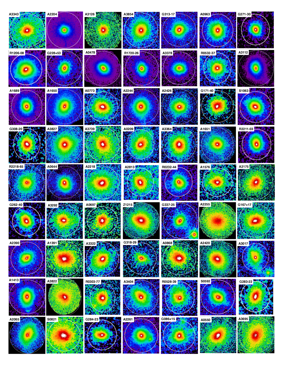
Figure J1: X-ray images of the galaxy clusters investigated in this paper, from the most relaxed to the most disturbed accordingly to the visual classification. The white circles indicate the estimated $R_{500}$.

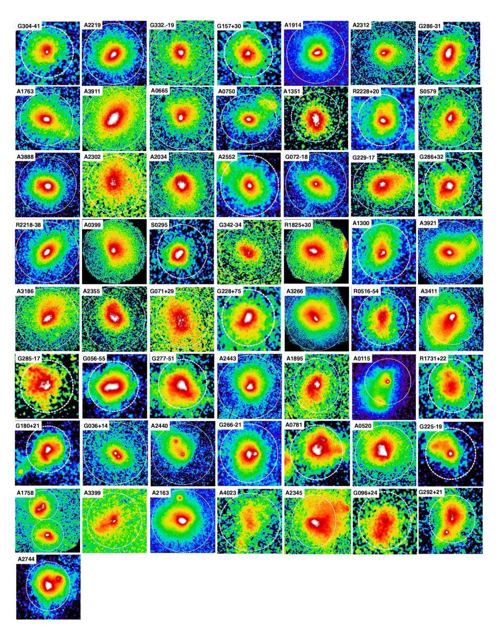
Figure J1: continued from the previous page.

References

- Abraham et al. (2003) Abraham, R. G., van den Bergh, S., & Nair, P. 2003, ApJ, 588, 218
- Andrade-Santos et al. (2012) Andrade-Santos, F., Lima Neto, G. B., & Laganá, T. F. 2012, ApJ, 746, 139
- Andrade-Santos et al. (2017) Andrade-Santos, F., Jones, C., Forman, W. R., et al. 2017, ApJ, 843, 76
- Angulo et al. (2012) Angulo, R. E., Springel, V., White, S. D. M., et al. 2012, MNRAS, 426, 2046
- Applegate et al. (2016) Applegate, D. E., Mantz, A., Allen, S. W., et al. 2016, MNRAS, 457, 1522
- Arnaud (1996) Arnaud, K. A. 1996, in Astronomical Society of the Pacific Conference Series, Vol. 101, Astronomical Data Analysis Software and Systems V, ed. G. H. Jacoby & J. Barnes, 17
- Arnaud et al. (2005) Arnaud, M., Pointecouteau, E., & Pratt, G. W. 2005, A&A, 441, 893
- Arnaud et al. (2010) Arnaud, M., Pratt, G. W., Piffaretti, R., et al. 2010, A&A, 517, A92
- Bartalucci et al. (2017) Bartalucci, I., Arnaud, M., Pratt, G. W., et al. 2017, A&A, 598, A61
- Böhringer et al. (2010) Böhringer, H., Pratt, G. W., Arnaud, M., et al. 2010, A&A, 514, A32
- Borm et al. (2014) Borm, K., Reiprich, T. H., Mohammed, I., & Lovisari, L. 2014, A&A, 567, A65
- Buote & Tsai (1995) Buote, D. A., & Tsai, J. C. 1995, ApJ, 452, 522
- Buote & Tsai (1996) —. 1996, ApJ, 458, 27
- Burenin et al. (2007) Burenin, R. A., Vikhlinin, A., Hornstrup, A., et al. 2007, ApJS, 172, 561
- Cassano et al. (2010) Cassano, R., Ettori, S., Giacintucci, S., et al. 2010, ApJ, 721, L82
- Cuciti et al. (2015) Cuciti, V., Cassano, R., Brunetti, G., et al. 2015, A&A, 580, A97
- Donahue et al. (2016) Donahue, M., Ettori, S., Rasia, E., et al. 2016, ApJ, 819, 36
- Eckert et al. (2017) Eckert, D., Ettori, S., Pointecouteau, E., et al. 2017, Astronomische Nachrichten, 338, 293
- Eckert et al. (2011) Eckert, D., Molendi, S., & Paltani, S. 2011, A&A, 526, A79
- Fakhouri et al. (2010) Fakhouri, O., Ma, C.-P., & Boylan-Kolchin, M. 2010, MNRAS, 406, 2267
- Hudson et al. (2010) Hudson, D. S., Mittal, R., Reiprich, T. H., et al. 2010, A&A, 513, A37
- Israel et al. (2014) Israel, H., Reiprich, T. H., Erben, T., et al. 2014, A&A, 564, A129
- Jones & Forman (1984) Jones, C., & Forman, W. 1984, ApJ, 276, 38
- Jones & Forman (1999) —. 1999, ApJ, 511, 65
- Lau et al. (2009) Lau, E. T., Kravtsov, A. V., & Nagai, D. 2009, ApJ, 705, 1129
- Lin et al. (2015) Lin, H. W., McDonald, M., Benson, B., & Miller, E. 2015, ApJ, 802, 34
- Lotz et al. (2004) Lotz, J. M., Primack, J., & Madau, P. 2004, AJ, 128, 163
- Lovisari et al. (2015) Lovisari, L., Reiprich, T. H., & Schellenberger, G. 2015, A&A, 573, A118
- Lovisari et al. (2011) Lovisari, L., Schindler, S., & Kapferer, W. 2011, A&A, 528, A60
- Mann & Ebeling (2012) Mann, A. W., & Ebeling, H. 2012, MNRAS, 420, 2120
- Mantz et al. (2015) Mantz, A. B., Allen, S. W., Morris, R. G., et al. 2015, MNRAS, 449, 199
- McDonald et al. (2017) McDonald, M., Allen, S. W., Bayliss, M., et al. 2017, ArXiv e-prints, arXiv:1702.05094
- Mohr et al. (1993) Mohr, J. J., Fabricant, D. G., & Geller, M. J. 1993, ApJ, 413, 492
- Motl et al. (2005) Motl, P. M., Hallman, E. J., Burns, J. O., & Norman, M. L. 2005, ApJ, 623, L63
- Nurgaliev et al. (2013) Nurgaliev, D., McDonald, M., Benson, B. A., et al. 2013, ApJ, 779, 112
- Nurgaliev et al. (2017) —. 2017, ApJ, 841, 5
- Parekh et al. (2015) Parekh, V., van der Heyden, K., Ferrari, C., Angus, G., & Holwerda, B. 2015, A&A, 575, A127
- Pinkney et al. (1996) Pinkney, J., Roettiger, K., Burns, J. O., & Bird, C. M. 1996, ApJS, 104, 1
- Planck Collaboration et al. (2011a) Planck Collaboration, Aghanim, N., Arnaud, M., et al. 2011a, A&A, 536, A9
- Planck Collaboration et al. (2011b) Planck Collaboration, Ade, P. A. R., Aghanim, N., et al. 2011b, A&A, 536, A8
- Planck Collaboration et al. (2013) —. 2013, A&A, 550, A130
- Planck Collaboration et al. (2014) —. 2014, A&A, 571, A20
- Pratt et al. (2009) Pratt, G. W., Croston, J. H., Arnaud, M., & Böhringer, H. 2009, A&A, 498, 361
- Randall et al. (2002) Randall, S. W., Sarazin, C. L., & Ricker, P. M. 2002, ApJ, 577, 579
- Rasia et al. (2013) Rasia, E., Meneghetti, M., & Ettori, S. 2013, The Astronomical Review, 8, 40
- Rasia et al. (2006) Rasia, E., Ettori, S., Moscardini, L., et al. 2006, MNRAS, 369, 2013
- Reiprich & Böhringer (2002) Reiprich, T. H., & Böhringer, H. 2002, ApJ, 567, 716
- Ricker & Sarazin (2001) Ricker, P. M., & Sarazin, C. L. 2001, ApJ, 561, 621
- Roncarelli et al. (2006) Roncarelli, M., Ettori, S., Dolag, K., et al. 2006, MNRAS, 373, 1339
- Rossetti et al. (2017) Rossetti, M., Gastaldello, F., Eckert, D., et al. 2017, MNRAS, 468, 1917
- Rossetti et al. (2016) Rossetti, M., Gastaldello, F., Ferioli, G., et al. 2016, MNRAS, 457, 4515
- Santos et al. (2008) Santos, J. S., Rosati, P., Tozzi, P., et al. 2008, A&A, 483, 35
- Smith et al. (2001) Smith, R. K., Brickhouse, N. S., Liedahl, D. A., & Raymond, J. C. 2001, ApJ, 556, L91
- Sunyaev & Zeldovich (1972) Sunyaev, R. A., & Zeldovich, Y. B. 1972, Comments on Astrophysics and Space Physics, 4, 173
- Tchernin et al. (2016) Tchernin, C., Eckert, D., Ettori, S., et al. 2016, A&A, 595, A42
- Ventimiglia et al. (2008) Ventimiglia, D. A., Voit, G. M., Donahue, M., & Ameglio, S. 2008, ApJ, 685, 118
- Vikhlinin et al. (2007) Vikhlinin, A., Burenin, R., Forman, W. R., et al. 2007, in Heating versus Cooling in Galaxies and Clusters of Galaxies, ed. H. Böhringer, G. W. Pratt, A. Finoguenov, & P. Schuecker, 48
- Weißmann et al. (2013) Weißmann, A., Böhringer, H., Šuhada, R., & Ameglio, S. 2013, A&A, 549, A19
- Willingale et al. (2013) Willingale, R., Starling, R. L. C., Beardmore, A. P., Tanvir, N. R., & O’Brien, P. T. 2013, MNRAS, 431, 394
- Zhang et al. (2009) Zhang, Y.-Y., Reiprich, T. H., Finoguenov, A., Hudson, D. S., & Sarazin, C. L. 2009, ApJ, 699, 1178