Exploiting Latent Attack Semantics for
Intelligent Malware Detection

Abstract.

We introduce a new malware detector – Shape-GD – that aggregates per-machine detectors into a robust global detector. Shape-GD is based on two insights: 1. Structural: actions such as visiting a website (waterhole attack) or membership in a shared email thread (phishing attack) by nodes correlate well with malware spread, and create dynamic neighborhoods of nodes that were exposed to the same attack vector. However, neighborhoods vary unpredictably and require aggregating an unpredictable number of local detectors’ outputs into a global alert. 2. Statistical: feature vectors corresponding to true and false positives of local detectors have markedly different conditional distributions – i.e. their shapes differ. We show that the shape of neighborhoods can identify infected neighborhoods without having to estimate the number of local detectors in the neighborhood.

We evaluate Shape-GD by emulating a large community of Windows systems – using system call traces from a few thousand malware and benign applications – and simulating a waterhole attack through a popular website and a phishing attack in a corporate email network. In both these scenarios, we show that Shape-GD detects malware early ($\sim$100 infected nodes in a $\sim$100K node system for waterhole and $\sim$10 of 1000 for phishing) and robust (with $\sim$100% global true positive and $\sim$1% global false positive rates). At such early stages of infection, existing algorithms that cluster feature vectors are ineffective (have an AUC metric of close to 0.5), and others that count the fraction of alert-generating local detectors require (the weakly correlated) neighborhoods’ sizes to be estimated to within 1% accuracy.

1. Introduction

Behavioral detectors are a crucial line of defense against malware. By extracting features out of network packets (wenkee_lee_bothunter_2007, ; paxson1999, ; Sommer2010, ; zhang2001, ), system calls (Canali2012, ; Christodorescu06, ; Fredrikson2010, ), instruction set (Juxtapp, ; Christodorescu05, ), and hardware (Demme2013, ; Tang2014, ; dmitry-ensemble, ) level actions, behavioral detectors train machine learning algorithms to classify program binaries and executions as either malicious or benign. In practice, behavioral detectors are deployed extensively as per-machine local detectors whose alerts are analyzed by global detectors  (cisco-amp, ; dell-ampd, ; osquery, ; GRR, ; hone, ; hone_code, ).

However, behavioral detectors are weak – i.e., have high false positives and negatives. This is because a large class of malware includes benign-looking behaviors, such as encrypting users’ data, use of obfuscated code, or making web/HTTP requests. Further, machine learning-based detectors have been shown to be susceptible to evasion attacks (evade-ml, ; evade-pdf, ; practical_black_box_attacks, ) that either increase false negatives or force detectors to output more false positives. As a result, global detectors in enterprises with $\sim$100K local detectors have to process millions of alerts per day (attack_graphs, ) which stresses heavy-weight program analyses and human analysts who investigate the final alerts (graphistry, ) – our goal is to build a robust global detector that amplifies weak local detectors.

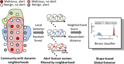
Figure 1. (L to R) Each circle is a node that runs a local malware detector (LD). Our goal is to create a robust global detector (GD) from weak LDs. We observe that nodes naturally form neighborhoods based on attributes relevant to attack vectors – e.g., all client devices that visit a website W within the last hour belong to neighborhood $NB_{w}$, or all users who received an email from a mailing list M in the last hour belong to neighborhood $NB_{m}$. We propose a new GD that groups together suspicious local feature vectors based on neighborhoods – traditional GDs only analyze local alerts while we re-analyze feature vectors that led to the alerts. Our GD then exploits a new insight – the conditional distribution of true positive feature vectors differs from false positive feature vectors – to robustly classify neighborhoods as malicious.

Challenges for prior work. Boosting weak detectors using purely machine learning techniques is challenging. The dominant approaches are (a) clustering: combine feature vectors using some distance metric to identify suspicious clusters of feature vectors (Seurat2004, ; beehive2013, ; bot_graph, ; bot_grep, ), and (b) counting: train local detectors (LDs) such as Random Forests to generate local alerts, and generate a global alert if there is a significant fraction of local alerts in the enterprise (Dash2006, ; BotSniffer, ; wenkee_lee_bothunter_2007, ; Shin_Infocom12_EFFORT, ). Both approaches have limitations that force enterprises to deploy brittle rule-sets that explicitly correlate local detector alerts.

Clustering algorithms are well-known to be highly sensitive to noise, especially in the high-dimensional regime (donoho1983notion, ; huber2011robust, ; xu2013outlier, ). Indeed, classical approaches that attempt to detect or to score ”outlyingness” of points (e.g. Stahel-Donoho outlyingness, Mahalanobis distance, minimum volume ellipsoid, minimum covariance determinant, etc) are fundamentally flawed in the high-dimensional regime (i.e., theoretically cannot guarantee correct detection with high probability). In practice, we see this in prior work (beehive2013, ) where clustering is used primarily as a first-level analysis to discover malicious incidents for a human analyst (i.e. requires lower accuracy than a global detector). In Appendix A we find that a clustering global detector is ineffective in early stages of infection where our detector succeeds – i.e., clustering yields an Area Under Curve (AUC) metric of only $\sim$ 48% against waterhole attack and phishing attacks.

Count-based global detectors (Count-GD), on the other hand, suffer because they need to know the size of local detector communities extremely accurately to determine whether a significant fraction is raising alerts. In practice though, these communities of local detectors are extremely ‘noisy’. For example, consider a community of machines in an enterprise who are potentially exposed to a so-called waterhole attack (waterhole_attack, ) (where a compromised webpage spreads malicious code to machines in the enterprise). Here, a malicious javascript-advertisement might be targeted by an ad-broker to only a fraction of visitors to a set of webpages. Further, the specific exploit might only succeed on a small fraction of machines that did receive the exploit because of browser versions or patching status. Surprisingly, our experiments show that if Count-GD underestimates the number of nodes where the exploit ran successfully (i.e., the community size) by just 2%, its alerts are almost 100% false positives (similarly, overestimating the community by 14% leads to almost 0% true positives). Even small errors in estimating the number of feature vectors in the community linearly affects the global detector’s decision thresholds.

Proposed Ideas – Neighborhood filtering and Shape. Our intuition is that a weak signal indicative of malicious behavior still separates true- and false-positive feature vectors, even though local detectors classify both as malicious. Our proposed system, Shape-GD, relies on two key insights to correctly identify malicious feature vectors.

First, attack vectors into a firewalled enterprise create short-lived and dynamic correlations across nodes – e.g., machines that visit a specific server (in watering hole attacks) or receive email from an address (in phishing attacks) are more likely to be compromised than a random machine in the community. Since an attacker cannot target a machine inside an enterprise directly, machines that have been exposed to a common attack vector have correlated alerts. We call such a set of machines a neighborhood. Neighborhoods thus concentrate the signal of malware activity that is otherwise not visible at the overall community level and can thus enable early detection of malware attacks. Neighborhoods are, however, extremely unpredictable and render cluster and count-based GDs ineffective – hence we propose Shape-GD to aggregate local detectors’ outputs.

The second insight behind Shape-GD is that the distributional shape of a set of suspicious feature vectors can robustly separate true positive neighborhoods from false positive neighborhoods. Shape-GD analyzes only those feature vectors that cause alerts by the local detectors (alert-FVs) instead of analyzing all feature vectors. Alert-FVs thus represent draws from one of two conditional distributions – i.e., distribution of malicious or benign feature vectors conditioned on being labeled as suspicious – which are similar but not the same. Next, while a single suspicious feature vector is uninformative, a set of such feature vectors can indeed be tested to come from one of two similar-but-distinct distributions. To conduct this hypothesis test, Shape-GD introduces a quantitative scoring function that maps a set of feature vectors (the alert-FVs per neighborhood) into one scalar value – the ShapeScore of the neighborhood.

Shape-GD composes the two insights – i.e., filters alert-FVs along neighborhood lines followed by computing the neighborhood’s shape – and achieves two key properties: (i) the distribution of the alert-FVs strongly separates malicious and benign neighborhoods (essentially, it separates the true positive alert-FVs from false positive alert-FVs), and (ii) is robust to noise in neighborhood size estimates (i.e., we do not need accurate neighborhood sizes and only need a sufficient number of alert-FVs to make a robust hypothesis test). Specifically, Shape-GD detects malicious neighborhoods with less than 1.1% and 2% compromised nodes per neighborhood (in two case studies involving waterhole and phishing attacks respectively), at a false positive and true positive rate of 1% and 100% respectively. Neighborhood filtering and ShapeScore complement each other – neighborhoods concentrate the weak signal into a small but unpredictable set of feature vectors while ShapeScore extracts this signal without knowing the precise number of feature vectors.

Contributions. Neighborhood filtering and shape enable structural information about attack vectors to be captured algorithmically. Our specific contributions are as follows.

• Neighborhood filtering to ‘reanalyze’ alert feature vectors instead of only alert time-series, and Shape-GD algorithms that exploit a new property – the statistical ‘shape’ of a neighborhood separates the ones with true positives from those with false positives – to classify neighborhoods as malicious or benign without knowing their size.

• An efficient detector that can identify malicious neighborhoods using only 15,000 feature vectors (roughly 15 seconds of data from a 1000-node neighborhood). The detector comprises of random forest LDs and a Shape-GD that computes ShapeScore as the Wasserstein distance between a set of alert-FVs’ histograms and a reference histogram built using false positive feature vectors (created by running LDs on benign programs in uninfected machines that are used to train the GD).

• Phishing case study. Shape-GD detects a phishing attack with 1% false positive rate in a medium size enterprise network with a neighborhood of 1086 nodes when only 17.08 nodes (using temporal neighborhoods) and 4.48 nodes (with additional mailing-list based structural filtering) are infected.

• Waterhole attack case study. Shape-GD detects a waterhole attack with 1% false positive rate when only 107.5 nodes (using temporal neighborhoods) and 139.9 (with additional server specific structural filtering) out of $\sim 550,000$ nodes are infected.

We emphasize that the LD and GD false positives (FPs) have very different interpretations. In a phishing attack, an LD FP of 1% in a neighborhood of 1000 nodes means that we will get about 10 FP alerts per second. The Shape-GD, on the other-hand, uses these LD FP alerts for decision making. Thus a GD false positive occurs when it misclassifies a neighborhood of LD alerts – a much rarer scenario.

Specifically, a GD FP rate of 1% means that in our phishing attack scenario, we will receive a global false alert about once every 100 - 300 hours. Similarly, in the waterhole scenario a global false positive occurs every 100 sec. Comparing the number of LDs’ FPs that are reported to a GD in a Count GD v. Shape-GD, temporal neighborhood filtering reduces total FPs by $\sim$100$\times$ (phishing) and $\sim$200$\times$ (waterhole), while adding structural filtering reduces total FPs by $\sim$1000$\times$ and $\sim$830$\times$ respectively (Appendix E for details).

Finally, as an auxiliary contribution, we present a methodology to evaluate detectors where the LD and GD algorithms are tightly integrated. Existing enterprise networks provide black-box LDs (such as Blue Coat, Symantec etc) that push alert logs into ‘SIEM’ tools (like Splunk) where GD algorithms and visualization tools are deployed. Section 5 describes the limitations of three real settings we have worked on – a real enterprise dataset, a university network test-bed, and the Symantec WINE dataset. None of these allow a GD to acquire alert feature vectors from LDs. Instead, we incorporate a host-level malware analysis setup (kruegel-bare-metal, ) into real enterprise data center (yahoo-G4, ) and email (enron-dataset, ) traces, vary the rates of infection systematically, and thus determine the operating range of Shape-GD agnostic of one specific sequence of events. This methodology offers a more robust measure of Shape-GD’s detection rate under adaptive malware that can alter its infection behavior in response to Shape-GD’s analysis.

2. Overview of Shape-GD

Threat model and Deployment. We assume a standard threat model where trusted local detectors (LDs) at each machine communicate with a trusted global detector (GD) that receives alerts and other metadata from the local detectors. The LDs are isolated from untrusted applications on local machines using OS- (e.g., SELinux) and hardware mechanisms (e.g., ARM TrustZone), and communicate with the enterprise’s GD through an authenticated channel. The GD is trained as a standard anomaly detector – using benign data generated from uninfected (e.g. test/quality-assurance) machines that run LDs on benign software, or assuming the current state of the system as benign in order to detect future malware as anomalies.

Shape-GD fits deployment models that are common today. Currently, enterprises use SIEM tools (like HP Arcsight and Splunk) to monitor network traffic and system/application logs, malware analysis sandboxes that scan emails for malicious links and attachments, in addition to host-based malware detectors (LDs) from Symantec, McAfee, Lookout, etc. We use exactly these side-information – from network logs (client-IP, server IP, timestamp) and email monitoring tools – to instantiate neighborhoods and filter LDs’ alert-FVs based on neighborhoods (Algorithm 2). Upon receiving alert-FVs, Shape-GD runs its malware detection algorithm (Algorithm 3) for all neighborhoods the alert-FVs belong to. If a particular neighborhood is suspicious, then Shape-GD will notify a downstream analysis (deeper static/dynamic analyses or human analysts) and forward relevant information in the incident report.

The key difference is that Shape-GD needs to know the alert feature vectors from the LDs – black-box LDs do not currently provide these. Hence (e.g., osquery-based) co-designed LD-GD detectors (osquery, ; GRR, ) are the most appropriate deployment counterpart for Shape-GD– this also motivates our experimental setup combining host-level malware analysis and web-service/email datasets.

Operationally, the LD at each machine transforms its input signal into an alert time series. This transformation consists of two steps: (a) Generate Feature Vectors: convert the raw OS system calls trace into a feature vector (FV) time series, and (b) Generate Alerts: Determine if each FV is malicious or not using a local detector (typically through random forests, SVM, etc.).

Inferring neighborhoods from common attack vectors. Shape-GD operates over dynamic neighborhoods, which are updated once per neighborhood time window (NTW). Neighborhoods within large communities are a set of nodes that share a statically defined action attribute within the current time window – this allows an analyst to create neighborhoods of nodes based on common attack vectors. Below are some illustrative examples of communities and neighborhoods – we focus our experiments on the first two examples that are responsible for a large fraction of malware in enterprises.

1. Waterhole attack. The community here consists of the employees of an enterprise such as Anthem Health (anthem, ; anthem-waterhole, ). In a waterhole attack, adversaries compromise a website commonly visited by such employees as a way to infiltrate the enterprise network and then spread within the network to a privileged machine or user. Within this community, a neighborhood can be the set of nodes that visited the same type of websites within the current neighborhood time window (for example, some percentile of suspicious links rated by VirusTotal (virustotal, ) or SecureRank (secure_rank, )). Since these rankings themselves are fuzzy, and the websites and their contents are dynamic, neighborhoods only indicate a probability that the node was actually exposed to an exploit.

2. Phishing attack over enterprise email networks. The community here consists of all employees within an enterprise. A phishing attack here would typically spread over email and use a malicious URL to lure nodes (users) to drive-by-download attacks (phishing-1, ; phishing-2, ) or spread through malicious attachments. Here, a specific user’s neighbors are that subset of users with whom she/he exchanged emails with during the current neighborhood time window.

Similar correlations occur in physical hardware attacks – community here consists of all machines in a workplace that are physically proximal (e.g. machines in a specific hospital or bank determined using the configuration of LAN/WiFi infrastructure, GPS information etc). The potential attack mode here is through physical hardware such as badUSB. The neighborhood of a node is simply all other nodes in the neighborhood that were connected to similar external hardware (e.g. a USB drive) over the current neighborhood time window.

Attacks that target specific app-stores (e.g., the Key-Raider attack in the Cydia app-store or the malicious Xcode attacks due to compromised mirror sites) also propagated across users with specific attributes (membership in a store or downloaded Xcode from specific sites) more likely than a random user in the network.

2.1. Intuition behind Shape-GD

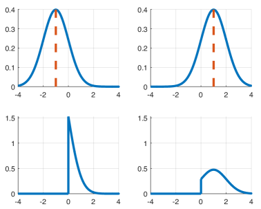
Figure 2. (Shape of conditional distributions) The top left figure is the probability density function (pdf) of benign feature vectors, here a Gaussian with mean ‘-1’; and the top right figure is the pdf for malicious feature vectors, here a Gaussian with mean‘+1’. The optimal local detector at any machine would declare ’malware’ if a sample’s value is positive, and declare ’benign’ if a sample’s value is negative. The bottom plots shows the pdfs of the same Gaussians but now conditioned on the event that the sample is positive – the pdfs corresponding to false positive and true positive feature vectors respectively have different shapes.

The statistical shape of local detectors’ false positives (FP conditional distribution) differs from the corresponding shape for true positives (TP conditional distribution) – we use this property to aggregate LDs’ alert-FVs to find the shape of each neighborhood and then classify neighborhoods based on their shapes.

The central question then is – why do true- and false-positive FVs’ shapes differ? To explain this and set the stage for Shape-GD, we consider a stylized statistical inference example. Suppose that we have an unknown number of nodes within a neighborhood. We want to distinguish between two extremes – all nodes only run benign applications (benign hypothesis), or all nodes are running malware (malware hypothesis). We look at a single snapshot of time where each node generates exactly one feature vector. Under the benign hypothesis, assume that the feature vector from each node is a (scalar valued) sample from a standard Gaussian with mean of ‘-1’; alternatively it is standard Gaussian with mean of ‘+1’ under the malware hypothesis.

(a) Noisy local detectors: Given one sample (i.e., FV from one node), the best local detector is a threshold test: is the sample’s value above zero or below? For this example, the probability of a false positive is (about) 15%.

(b) Aggregating local detectors over neighborhoods: Suppose there are 100 nodes and all of them report their value, and we are told that 90 of them are greater than 0 (i.e., 90 of the local detectors generate alerts). In this case, the expected number of alerts under the benign hypothesis is 15; and 85 under the malware hypothesis. Thus, we can conclude with overwhelming certainty ($10^{-75}$ chance of error) that 90 alerts indicate an infected neighborhood. This corresponds to a conventional threshold algorithm that count the number of alarms in a neighborhood and compares with a global threshold (here this threshold is 50).

(c) Count without knowing neighborhood size: Suppose, now, that we do not know the number of nodes (i.e., neighborhood size is unknown), and only know that there are a total of 90 alerts. In other words, out of the neighborhood of nodes, some 90 of them whose samples were positive reported so. What can we say? Unfortunately we cannot say much – if there were 100 nodes in neighborhood, then malware is extremely likely; however, if there were 1000 total nodes, then with 90 alerts, it is by far (exponentially) more likely that we have no infection. Because we do not know the neighborhood size, the global threshold cannot be computed.

(d) Robustness of Shape: While the number of alerts alone is uninformative, we can resolve whether the neighborhood is a ‘false positive’ or ‘true positive’ by considering the actual values of the 90 random variables corresponding to these alerts. These values represent independent draws from a conditional distribution – either the distribution of a normal random variable of mean ’$-1$’ conditioned on taking a nonnegative value, or the distribution of a normal random variable of mean ’$+1$’ conditioned on taking a nonnegative value (see Figure 2). This conditioning occurs because of the local detector – recall it tags a sample as an alert if and only if the sample drawn was nonnegative (optimal LD in this example). Thus, irrespective of the size of the neighborhood, the global detector would “look at the shape” of the empirical distribution (i.e. the distribution constructed from the received samples) of the received samples (FVs). If this were “closer” to the left rather than the right plot in Figure 2, it would declare “uninfected”; otherwise declare “infected”.

2.2. From Intuition to Algorithm Design

Interestingly, we show that the intuition behind this simple example scales to real malware detectors that use high-dimensional feature vectors. However, to use this insight in practice, we need to address two issues: (i) while the two figures in Figure 2 are visually distinct, an algorithmic approach requires a quantitative score function to separate between the (vector-valued) conditional distributions generated from feature vector samples; and (ii) the global detector receives only finitely many samples; thus, we can construct (at best) only a noisy estimate of the conditional distribution. We describe Shape-GD’s details in Section 4 but present the key intuition here.

We introduce ShapeScore – a score function based on the Wasserstein distance (wasser-wiki, ) to resolve between conditional distributions. We choose Wasserstein distance because it has well-known robustness properties to finite-sample binning (vallender1974calculation, ; benbre00, ), was more discriminative than L1/L2 distances in our experiments, and yet is efficient to compute for vectors.

Specifically, given a collection of feature vector samples, we construct an empirical (vector) histogram of the FV samples, and determine the Wasserstein distance of this histogram with respect to a reference histogram. This reference histogram is constructed from the feature vectors corresponding to the false positives of the local detectors. In other words, this reference histogram captures the statistical shape of the “failures” of the LDs – i.e., those FVs that the LD classifies as malicious even though they arise from benign applications. Computing the reference histogram does not require analysts to manually label alert-FVs as false positives – these can be generated by running the LDs on benign software in uninfected machines (e.g., test or quality-assurance machines, by recording and replaying real user traces on benign applications on training servers, etc). Alternatively, analysts can use applications deployed currently and recompute the reference histogram periodically – this is similar to anomaly detectors where the goal is to label anomalous behaviors as (potentially) malicious.

If we had the idealized scenario of infinite number of feature vector samples, the ShapeScore would be uniquely and deterministically known. In practice however, we have only a limited number of feature vector samples; thus ShapeScore is noisy. Our experiments (Figure 3) test its robustness with Windows benign and malicious applications (Section 6), where the ShapeScore is computed from neighborhood sizes of 15,000 FVs (about 15 seconds of data from 1000 nodes). The key result is the strong statistical separation between the ShapeScores for the TP and FP feature vectors respectively, thus lending credence to our approach. Importantly, both these ideas do not depend on knowing the neighborhood size; thus they provide a new lens to study malware at a global level.

3. Related Work

3.1. Behavioral analysis

Behavioral analysis refers to statistical methods that monitor signals from program execution, extract features and build models from these signals, and then use these models to classify processes as malicious. Importantly, as we discuss in this section, all known behavioral detectors have a high false positive and negative rate (especially when zero-day and mimicry attacks are factored in).

System-calls and middleware API calls have been studied extensively as a signal for behavioral detectors (Forrest1996, ; Wagner2002, ; kruegel2007, ; Christodorescu:2008:MSM:1342211.1342215, ; Fredrikson2010, ; Canali2012, ; robertson_anomaly, ). Network intrusion detection systems (paxson1999, ) analyze network traffic to detect known malicious or anomalous behaviors. More recently, behavioral detectors use signals such as power consumption(clark2013, ), CPU utilization, memory footprint, and hardware performance counters(Demme2013, ; Tang2014, ).

Detectors then extract features from these raw signals. For example, an n-gram is a contiguous sequence of n items that captures total order relations (BotSniffer, ; Canali2012, ), n-tuples are ordered events that do not require contiguity, and bags are simply histograms. These can be combined to create bags of tuples, tuples of bags, and tuples of n-grams (Canali2012, ; Forrest1996, ) often using principal component analysis to reduce dimensions. Further, system calls with their arguments form a dependency graph structure that can be compared to sub-graphs that represent malicious behaviors (Christodorescu:2008:MSM:1342211.1342215, ; Kolbitsch:2009:EEM:1855768.1855790, ; kruegel2007, ).

Finally, detectors train models to classify executions into malware/benignware using supervised (signature-based) or unsupervised (anomaly-based) learning. These models range from distance metrics, histogram comparison, hidden markov models (HMM), and neural networks (artificial neural networks, fuzzy neural networks, etc.), to more common classifiers such as kNN, one-class SVMs, decision trees, and ensembles thereof.

Such machine learning models, however, result in high false positives and negatives. Anomaly detectors can be circumvented by mimicry attacks where malware mimics system-calls of benign applications (Wagner2002, ) or hides within the diversity of benign network traffic(Sommer2010, ). Sommer et al. (Sommer2010, ) additionally highlights several problems that can arise due to overfitting a model to a non-representative training set, suggesting signature-based detectors as the primary choice for real deployments. Unfortunately, signature-based detectors cannot detect new (zero-day) attacks. On Android, both system calls (Burguera2011, ) and hardware-counter based detectors (Demme2013, ) yield $\sim$20% false positives and $\sim$80% true positives.

Finally, with their ability to extract highly effective features, deep nets may provide a new way forward for creating novel behavioral detectors. At the global level, however, what is needed is a data-light approach for global detection by composing local detectors, tailored to be agile enough to do global detection in a fast-changing (non-stationary) environment.

3.2. Collaborative Intrusion Detection Systems (CIDS)

Collaborative intrusion detection systems (CIDS) provide an architecture where LDs’ alerts are aggregated by a global detector (GD). GDs can use either signature-based or anomaly-based(zhang2001, ; vlachos2004, ), or even a combination of the two (krugel2001, ) to generate global alerts. Additionally, the CIDS architecture can be centralized, hierarchical, or distributed (using a peer-to-peer overlay network) (zhang2001, ).

In all cases, existing GDs use some variant of either clustering or count-based algorithms to aggregate LDs’ alerts. Count-based GD raises an alert once the number of alerts exceeds a threshold within a space-time window, while clustering-based GD may apply some heuristics to control the number of alerts  (Dash2006, ; Seurat2004, ; BotSniffer, ; wenkee_lee_bothunter_2007, ; Shin_Infocom12_EFFORT, ). In HIDE (zhang2001, ), the global detector at each hierarchical-tier is a neural network trained on network traffic information. Worminator(Locasto2005, ) additionally uses bloom filters to compact LDs’ outputs and schedules LDs to form groups in order to spread alert information quickly through a distributed system. All count- and clustering-based algorithms are fragile when the noise is high (in the early stages of an infection) and when the network size is uncertain. In contrast, our neighborhood filtering and shape-based GD is robust against such uncertainty.

Note that distributed CIDSs are vulnerable to probe-response attacks, where the attacker probes the network to find the location and defensive capabilities of an LD (Shmatikov2007, ; Bethencourt2005, ; Shinoda2005, ). These attacks are orthogonal to our setting since we do not have fixed LDs (i.e. all nodes are LDs).

4. Shape GD Algorithm

Our algorithm consists of feature extraction, local detector (LD), and the global detector (GD). Our key innovations are in the GD, however, we also discuss feature extraction and LD design for completeness.

Input : Sequence of executed system calls

Output : Alert-FVs

1 Let $id$ be LD’s identifier

2

3while True do

4      

5      $syscall$-$hist$ $\leftarrow$ $r$-sec histogram of system calls

6      

7      $syscall$-$hist_{PCA}$ $\leftarrow$ project $syscall$-$hist$ on $L$-dim PCA basis

8      

9      $label$ $\leftarrow$ BinaryClassifier($syscall$-$hist_{PCA}$);

10      if $label=malicious$ then

11             $alert$-$FV$ $\leftarrow$ $syscall$-$hist_{PCA}$

12             send $<alert$-$FV$, $id>$ to Shape-GD

13            

14      

Algorithm 1 Local Detector

Feature Extraction algorithm. This algorithm transforms the continuously evolving 390-dimensional time-series of Windows system calls into a discrete-time sequence of feature-vectors (FVs). This is accomplished by chunking the continuous time series into $r-$second intervals, and representing the system call trace over each interval as a single $L-$dimensional vector (Algorithm 1, lines 3–4). $L$ is typically a low dimension, reduced down from 390 using PCA analysis, to (in our experiments) $L=10$ and $r=1$ second.

Local Detector (LD) Algorithm. The LD algorithm (Algorithm 1) leverages the current state-of-the-art techniques in automated malware detection to generate a sequence of alerts from the FV sequence. Specifically, using both its internal state and the current FV, the LD algorithm generates an alert if it thinks that this FV corresponds to malware, and produces no alert if it thinks that the current FV is benign (lines 5–8). Henceforth, we define an alert-FV to be an FV that generates an LD alert (either true or false positive). In our experiments each LD employs Random Forest as a binary classifier for malware detection because Random Forest achieves the best performance on the training data set among the classifiers from a prior survey (Canali2012, ) and have been shown to be robust to adversarial inputs – we pick an operating point of 92.4% true positives at a false positive rate of 6% from the LD’s ROC curve (which is similar to detection rates in prior work (Canali2012, )). We have described our experiments with picking the best LD from a prior survey (Canali2012, ) in Appendix B and Figure 12.

Neighborhood Instances from Attack-Templates. Each neighborhood time window (NTW), Shape GD generates neighborhood instances (Algorithm 2) based on statically defined attack vectors – each attack vector is a “Template” to generate neighborhoods with. Algorithm 2 shows how the concept of neighborhood unifies operationally distinct attacks like waterhole and phishing.

The template for detecting a waterhole attack forms a neighborhood out of client nodes that access a server or a group of servers within a neighborhood time window. The other template, which is used for detection of a phishing attack, includes in a neighborhood email recipient machines belonging to a set of mailing lists. The two templates are shown in lines 3–10.

Input : Template-type, NTW

Output : Set of active neighborhoods NBDs

1 [time, time+NTW] defines the current time window

2 time $\leftarrow$ current time

3

4while True do

5       if Template-type = $waterhole\ attack$ then

6             $V$ := client machines*

7             $S$ := accessed servers*

8             predicate(A:Client, B:Servers) := $A$ accesses $B$

9            

10       else if Template-type = $phishing\ attack$ then

11             $V$ := email recipient machines*

12             $S$ := mailing lists*

13             predicate(A:Recipient, B:Mailing list) := $A$ $\subseteq$ $B$

14            

15      

16      partitioning a set into non-disjoint sets to incorporate

17       structural filtering

18       ${P_{1},P_{2},...,P_{N}}$ $\leftarrow$ partition-set($S$), where $S$ = $\bigcup\limits_{i=1}^{N}P_{i}$

19      

20      form neighborhoods $NB_{i}$ using partitions $P_{i}$

21       $NB_{i}$ $\leftarrow$ $\{V|$ predicate($V$, $P_{i}$)$\}$

22      

23      set expiration time for a neighborhood $NB_{i}$

24       $NB_{i}$.expiration-time $\leftarrow$ t+NTW

25      

26      add all neighborhoods to the set $NBDs$

27       $NBDs$ $\leftarrow$ $\{NB_{i}$ $|$ $\forall i$ in $[1,N]\}$

28      

29      advance time by NTW sec

30       time $\leftarrow$ time+NTW

31      

32*active within the time window [time, time+NTW]

Algorithm 2 Neighborhoods from Attack-Vectors

For simplicity we present a batch version of the neighborhood instantiation algorithm (Algorithm 2) which advances time by NTW and creates new neighborhoods for each NTW. In contrast, the online Shape GD version updates already existing neighborhoods while monitoring client–server interactions in real-time – we demonstrate the online Shape GD algorithm to detect waterhole attacks and the batch version against phishing attacks in our evaluation.

The neighborhood instantiation algorithm accepts a template type as input, i.e. either a template for detecting a waterhole attack or a phishing attack, and duration of an NTW. The algorithm runs once per NTW – starting by defining the sets $V$ and $S$ that will be used to form neighborhoods. For a waterhole attack, the set $V$ includes all client machines accessing a set of servers and $S$ is a set of the accessed servers. To instantiate neighborhoods for a phishing attack, $V$ is a set of all email recipient machines and $S$ is a set of mailing lists. In both cases the algorithm considers only the entities that are active within a current NTW window.

Each attack requires a predicate that determines relation between the elements of the sets $V$ and $S$. For a waterhole attack such a predicate is true if a client accesses one of the servers (line 6). In the case of a phishing template, the predicate is evaluated to true if a recipient belongs to a particular mailing list (line 10).

The neighborhood instantiation algorithm proceeds with partitioning the set $S$ into one or more disjoint subsets $P_{i}$ (line 11). This is to incorporate ‘structural filtering’ into the algorithm, allowing an analyst to create neighborhoods based on subsets of servers (instead of all servers in case of waterhole) or divide all mailing lists into subsets of mailing lists (in the phishing). Structural filtering boosts detection under certain conditions (see Section 6.3).

The neighborhood instantiation algorithm builds a neighborhood for each partition $P_{i}$ using a corresponding predicate (line 12). After forming a neighborhood, the algorithm sets its expiration time (line 13), which is the end of the current NTW window. All the neighborhoods in the set $NBDs$ are discarded at the end of the current NTW window. Finally, the algorithm adds the just formed neighborhoods to $NBDs$ (line 14) and advances time by one NTW (line 15).

The template-based neighborhood instantiation algorithm (Algorithms 2) shares the $NBDs$ data structure with the Algorithm 3 that uses neighborhoods’ shapes to detect malware.

Malware Detection in a Neighborhood. Algorithm 3 detects malware per neighborhood instead of individual nodes. The input to the algorithm is a set of alert-FVs from each neighborhood and its output is a global alert for the neighborhood. We now describe how the algorithm distinguishes between the conditional distributions of alert-FVs from true-positive and false positive neighborhoods.

The key algorithmic idea is to first extract neighborhood-level features – i.e., to map all alert-FVs within a neighborhood to a single vector-histogram which robustly captures the neighborhood’s statistical properties. Then, Shape GD compares this vector-histogram to a reference vector-histogram (built offline during training) to yield the neighborhood’s ShapeScore. The reference vector-histogram is constructed from a set of false positive alert-FVs – thus, it captures the statistical shape of misclassifications (FPs) by the LDs but at a neighborhood scale. Finally, Shape-GD trains a classifier to detect anomalous ShapeScores as malware. This is a key step in Shape-GD – i.e., mapping alert-FVs from a neighborhood into a single vector-histogram and then into a discriminative yet robust ShapeScore lets us analyze the joint properties of all alert-FVs generated within a neighborhood without requiring the FVs to be clustered or alerts to be counted. We describe these steps in further detail.

Input : $L$-dim projections of alert-FVs

Output : Malicious neighborhoods

1 Let $NBDs$ be a set of neighborhoods

2

3for each NB in NBDs do

4       aggregate L-dim projections of alert-FVs on per neighborhood basis

5       $B$ $\leftarrow$ $\{alert-FVs$ $|$ node $id$ $\subseteq$ $NB\}$

6      

7      build an $(L,b)$-dim. vector-histogram

8       $H_{B}\leftarrow$ bin & normalize $B$ along each dimension

9      

10      compute a neighborhood score – ShapeScore

11       $ShapeScore$ $\leftarrow$ Wasserstein Dist.($H_{B}$, $H_{{\rm ref}}$)

12      

13      perform hypothesis testing

14       if $ShapeScore>\gamma$ then

15             label $NB$ as malicious

16            

17      

Algorithm 3 Malware Detection in a Neighborhood

Generating histograms from alert-FVs. The algorithm aggregates $L$-dimensional projections of alert-FVs on per neighborhood basis into a set $B$ (Algorithm 3, line 3). After that, Shape GD converts low dimensional representation of alert-FVs, the set $B$, into a single $(L,b)$-dimensional vector-histogram denoted by $H_{B}$ (line 4). The conversion is performed by binning $L$-dimensional vectors within the $B$ set along each dimension. In each of the L-dimensions, the scalar-histogram of the corresponding component of the vectors is binned and normalized. Effectively, a vector-histogram is a matrix $L$x$b$, where $L$ is the dimensionality of alert-FVs and $b$ is the number of bins per dimension.

We use standard methods to determine the size and number of bins and note that the choice of Wasserstein distance in the next step makes Shape GD robust against variations due to binning. In particular, we tried square-root choice, Rice rule, and Doane’s formula (binning, ) to estimate the number of bins, and we found that 20–100 bins yielded separable histograms (as in Figure 3) for the Windows dataset and fixed it at 50 for our experiments.

ShapeScore. We get the ShapeScore by comparing this histogram, $H_{B}$, to a reference histogram, $H_{{\rm ref}}$, which is generated during the training phase using only the false positive FVs of the LDs. We run LDs on the system-call traces generated by benign apps – the FVs corresponding to the alerts from the LD (i.e., the false positives) are then used to construct the reference histogram $H_{{\rm ref}}.$ ShapeScore is thus the distance of a neighborhood from a benign reference histogram – a high score indicates potential malware.

To collect known benign traces, a straightforward approach is to use test inputs on benign apps or use record-and-replay tools to re-run real user inputs in a malware-free system. Or, like any anomaly detector, an enterprise can train Shape-GD using applications deployed currently and recompute $H_{ref}$ periodically.

The ShapeScore of the accumulated set of FVs, $B$, is given by the sum of the coordinate-wise Wasserstein distances (vallender1974calculation, ) (Algorithm 3, line 5) between

$$H_{B}=(H_{B}(1)\ H_{B}(2)\ \ldots\ H_{B}(L))$$

and

$$H_{{\rm ref}}=(H_{{\rm ref}}(1)\ H_{{\rm ref}}(2)\ \ldots\ H_{{\rm ref}}(L)).$$

In other words,

$${\rm ShapeScore}=\sum_{l=1}^{L}d_{W}(H_{B}(l),H_{{\rm ref}}(l)),$$

where for two scalar distributions $p,q,$ the Wasserstein distance (vallender1974calculation, ; wasser-wiki, ) is given by

$$d_{W}(p,q)=\sum_{i=1}^{b}\left|\sum_{j=1}^{i}\left(p(j)-q(j)\right)\right|.$$

This Wasserstein distance serves as an efficiently computable one dimensional projection, that gives us a discriminatively powerful metric of distance (vallender1974calculation, ; benbre00, ). Because the Wasserstein distance computes a metric between distributions – for us, histograms normalized to have total area equal to 1 – it is invariant to the number of samples that make up each histogram. Thus, unlike count-based algorithms, it is robust to estimation errors in community size. Figure 3 verifies this intuition, and shows that true positives and false positive feature vectors separate well when viewed through the ShapeScore.

Finally, to determine whether a neighborhood has malware present we perform hypothesis testing. If ShapeScore is greater than a threshold $\gamma$, we declare a global alert, i.e., the algorithm predicts that there is malware in the neighborhood (lines 6–7). The robustness threshold $\gamma$ is computed via standard confidence interval or cross-validation methods with multiple sets of false-positive FVs (see Section 6.1).

Computing Shape GD’s parameters. Here we elaborate on the steps that should be taken in a real world environment to choose parameters. The steps discussed here are generic and are applicable to other attacks beyond waterhole and phishing – the following results section quantifies each of these steps.

First, an analyst should start with designing an appropriate algorithm to run on local detectors (LDs) (Appendix B). To achieve this, an analyst needs to compare the performance of multiple feature extraction (FE) algorithms combined with a diverse set of machine learning classifiers. One way to choose the best pair of a FE algorithm and a classifier is to build ROC curves for each pair, and select the pair that meets the desired detection rate to computation/training effort for the LD.

Second, the analyst needs to determine whether even a purely malicious neighborhood can be separated from benign ones, and the minimum number of FVs per neighborhood to do so (Sections 6.1 and Appendix C). This number depends on the false positive rate of LDs ( e.g., in our experiments, we determined that a neighborhood should generate at least 15K FVs, see Figure 13).

Third, we need to choose an NTW based on the false positive rate (FP) and the desired time-to-detection (Section 6.2. A small NTW means more frequent transfers of FVs from LD to GD, whereas a long NTW means that more nodes can get compromised before the GD makes a decision and/or FPs can drown out TPs. Similarly, structural filtering can improve detection rate if the true positive alert-FVs are not deluged by the rate of false-positive alert-FVs – Section 6.3 quantifies how this trade-off differs for waterhole and phishing.

5. Experimental Setup

5.1. Case for a New Methodology

Shape-GD experiments require datasets where the global detector can acquire alert-FVs from local detectors, similar to osquery-based systems where the LD and GD are co-designed. We describe our experience with three existing methodologies and datasets – none of them allow alert-FVs to be acquired, provide complete ground truth infection information, or allow the infection rate to be varied. This motivates the methodology we use to systematically evaluate Shape-GD.

Analysis of existing datasets. Prior work has used enterprise logs (mining_log_data_alina_oprea, ) that are unavailable publicly. We have acquired similar security logs from a Fortune 500 company with a 200K machine network – the logs average 250M entries per day over a 2 year period, arise from 20 closed-source endpoint local detectors such as Symantec, McAfee, Blue Coat, etc, have almost 500 sparsely populated dimensions per log entry, and about 75% of the log entries lack important identity and event-timestamp information and are delayed by up to 60 days. Commercial (black-box) LDs do not expose feature vectors for external analysis.

We have also acquired network pcap traces from our university network, emulating prior work (network_intrusion_detection, ) in network-only global detectors. University security groups (like ours) are only allowed to collect network-layer pcap information for a rolling 2-week period and cannot instrument host machines (that are owned by students and visitors) – i.e., our 4TB/day dataset from 150K machines is unsuitable to evaluate Shape-GD because it doesn’t have LDs. Extending this dataset with a weak LD – the ability to inspect executables in a sandbox downloaded by hosts (e.g., as pursued by Lastline (lastline, )) – would be an appropriate experimental setup but sensitive data issues make such datasets hard to get. Hence, we model this extended setup in our methodology.

We have analyzed Symantec’s WINE dataset (downloader_graphs, ) and found it inadequate to evaluate Shape-GD even after layering VirusTotal information on it. Specifically, the WINE dataset includes downloader graphs (downloader_graphs, ) – the nodes are executables and the edges represent whether the source downloaded the destination executable – and represent downloader trojans (‘droppers’) in malware distribution networks (malware_distribution_net, ) that download payloads to steal information, encrypt the disk, etc on to the host. This dataset covers 5 years of data with 25M files (specifically, hashes that represent files) on over 1M machines – however, only 1.5M of the 25M hashes have reports on VirusTotal. Hence, one cannot reconstruct (alert) feature vectors for the hashes stored in the downloader graph.

Shape-GD re-analyzes (local) alert feature vectors in the global detector – filtering alert-FVs into neighborhoods and then computing the neighborhoods’ shapes. Hence we model osquery-like deployments as used in enterprises like Facebook and Google where the LDs and GDs are co-designed and GDs can acquire alert-FVs.

Simulating malware propagation in a network. Methodologies that use existing datasets with malware propagation (like the ones above) have an inherent weakness. Such datasets have one sequence of malware propagation events “hardwired” into the dataset and do not allow us to analyze how a detection mechanism reacts to variations of malware propagation dynamics, especially when malware can adapt these dynamics. Instead, we propose to vary the rate of infection (which changes the neighborhood formation) and determine Shape-GD’s detection performance across different infection rates.

Further, none of the above datasets provide ground truth information about the true extent of infections, incentivizing a design that minimizes false positives at the expense of false negatives. In a controlled setting where host-level malware and benignware traces are overlaid onto a trace of web-service/email communication, we can maintain ground truth information and determine false positives and negatives precisely.

To this end, we use a malware and benignware dataset from a recent related work (kruegel-bare-metal, ), train an LD with histogram-based feature vectors and a Random Forest detector based on a recent survey on host-level malware detection (Canali2012, ), and overlay these host-level results on web-service (network) and email traces using two standard (and publicly available) datasets from Yahoo data centers and Enron respectively. We describe this methodology in detail next.

5.2. Benign and Malware Applications

We collect data from thousands of benign applications and malware samples. To avoid tracing program executions where malware may not have executed any stage of its exploit or payload correctly, we set a threshold of 100 system calls per execution to be considered a success. Our experiments successfully run 1,311 malware samples from 193 malware families collected in July 2013 (kruegel-bare-metal, ), and 2,364 more recent samples from 13 popular malware families collected in 2015 (kaspersky-windows-2015, ), to compare against traces from 1,889 benign applications.

We record time stamped sequences of executed system calls using Intel’s Pin dynamic binary instrumentation tool. Each Amazon AWS virtual machine instance runs Windows Server 2008 R2 Base on the default T2 micro instances with 1GB RAM, 1 vCPU, and 50GB local storage. The VMs are populated with user data commonly found on a real host including PDFs, Word documents, photos, Firefox browser history, Thunderbird calendar entries and contacts, and social network credentials. To avoid interference between malware samples, we execute each sample in a fresh install of the reference VM. As malware may try to propagate over the local network, we set up a sub-net of VMs accessible from the VM that runs the malware sample. In this sub-net, we left open common ports (HTTP, HTTPS, SMTP, DNS, Telnet, and IRC) used by malware to execute its payload. We run each benign and malware program 10 times for 5 minutes per run for a total of almost 53,000 hours total compute time on Amazon AWS.

Overall, benignware and malware were active for 141,670 sec and 283,270 seconds respectively, executing an average of 11,900 and 13,500 system calls per second respectively. Using 1 second time window (Section 4) and sliding the time windows by 1ms, we extract histograms of system calls within each time window as the ML feature, and finally pick 1.5M benign and 1M malicious FVs from this dataset for the experiments that follow. Importantly, we do not constrain the samples on neighboring machines to belong to the same families – as described above, malware today predominantly spreads through malware distribution networks where a downloader trojan (‘dropper’) can distribute arbitrary and unrelated payloads on hosts. We want to test Shape-GD in the extreme case where malicious FVs can be assigned from any malware execution to any machine.

5.3. Modeling Waterhole and Phishing Attacks

Waterhole attack. To model a waterhole attack, we use Yahoo’s “G4: Network Flows Data” (yahoo-G4, ) dataset, which contains communication data between end-users and Yahoo servers. The 41.4 GB (in compressed form) of data were collected on April 29-30, 2008. Each netflow record includes a timestamp, source/destination IP address, source/destination port, protocol, number of packets and the number of bytes transferred from the source to the destination. We model the setting where heuristics such as SecureRank (secure_rank, ) are applied to identify suspicious servers and we assume that Shape-GD monitors the top (here, 50) suspicious servers based on SecureRank’s scores. Specifically, we use 5 hours of network traffic (208 million records) captured on April 29, 2008 between 8 am and 1 pm at the border routers connecting Dallas Yahoo data center (DAX) to the Internet. The selected 50 DAX servers communicate with 3,181,127 client machines over 14,249,931 requests.

We assume that an attacker compromises one of the most frequently accessed DAX server – 118.242.107.76, which processes $\sim 752,000$ requests within 5-hour time window ($\sim 43.7$ requests per second). In our simulation it gets compromised at random instant between 8am and 10.30am. Hence, Shape GD can use the remaining 2.5 hours to detect the attack (our results show that less than a hundred seconds suffice). Following infection, we simulate this ‘waterhole’ server compromising client machines over time with an infection probability parameter – this helps us determine the time to detection at different rates of infection. The benign and compromised machines then select corresponding type of execution trace (i.e., a sequence of FVs generated in Section 5.2) and input these to their LDs.

Phishing attack. We simulate a phishing attack in a medium size corporate network of 1086 nodes that exchange emails with others in the network. To model email communication, we pick 50 email threads with 100 recipients each from the publicly available Enron email dataset (enron-dataset, ) (the union of all email threads’ recipients is 1086).

We start the simulation with these 50 emails being sent into the 1086-node neighborhood, and seed only one email out of 50 as malicious. We then model the infection speading at different rates as this malicious email is opened by its (up to 100) recipients at some time into the simulation and is compromised with some likelihood when the user ‘clicks’ on the URL in the email. Our goal is to measure the number of compromised nodes before Shape GD declares an infection in this neighborhood. All nodes that open and ‘click’ the link in the malicious email will select malware FVs from Section 5.2 as input to their corresponding LDs, while the remaining nodes select benign FVs.

To simulate the infection spreading over the email network, we need to (a) model when a recipient ‘opens’ the email: we do so using a long tail distribution of reply times where the median open time is 47 minutes, 90-percentile is one day, and the most likely open time is 2 minutes (email-resp-dist, ); and (b) model the ‘click’ rate (probability that a recipient clicks on a URL): we vary it from 0% up to 100% to control the rate of infection. For example, within 1-, 2-, 3-hour long time interval only 55%, 65%, and 70% of recipients of a malicious email open it, which corresponds to 55, 65, and 75 infected machines respectively at 100% click rate.

Overall, these two scenarios differ in their time-scales (seconds v. hours) and in the relative rate at which benign and malicious neighborhoods grow. As we will see, these parameters have a significant impact on the composition of neighborhoods and the Shape GD’s detection rate.

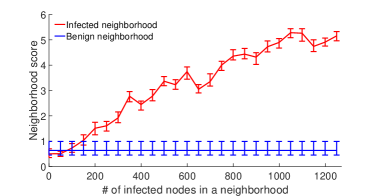
Figure 5. (Waterhole attack: Time-based NF) Dynamics of an attack: While the portion of infected nodes in a neighborhood increases over time reaching 1248 nodes on average, ShapeScore goes up showing that Shape GD becomes more confident in labeling neighborhoods as ‘malicious’. It starts detecting malware with at most 1% false positive rate when roughly 200 nodes get compromised. The neighborhood includes 17,178 nodes on average and spans over 30 sec time interval.

Methodology. We report averaged results from repeating each experiment multiple times with random initialization parameters. In particular, we use 10-fold cross validation for machine learning experiments (Figure 12), 500 randomly sampled benign/malicious neighborhoods with 10 repetitions to compute average (Figures 3, 13), 100 repetitions of each malware infection experiment (Figures 4,5,15,10), and 100 repetitions of infection with 10 repetitions per data-point (Figures 6,7,8,9). To train the reference histogram, $H_{{\rm ref}}$, we select 15K FVs and 100K FVs from the training data set in the phishing and waterhole experiments respectively. All Shape GD’s parameters are chosen based on a training data set (used for Figures 3 and 13) – we then evaluate Shape GD (in the remaining figures) using a completely separate testing data set.

6. Results

We show that Shape-GD can identify malicious neighborhoods with less than 1% false positive and 100% true positive rate when the neighborhoods produce more than 15,000 FVs within a neighborhood time window (i.e., $|B|>15,000$ in Algorithm 3). Recall that at 60 FVs/node/minute, it takes 1000 nodes only 15 seconds to create 15,000 FVs. For LDs like ours with $\sim$6% false positive rate, this corresponds to 900 alert-FVs. We then simulate realistic attack scenarios and find that Shape-GD can detect malware when only 5 of 1086 nodes are infected through phishing in an enterprise email network, and when only 108 of 550K possible nodes are infected through a waterhole attack using a popular web-service. Finally, Shape-GD is computationally efficient – we relegate this discussion to Appendix D.

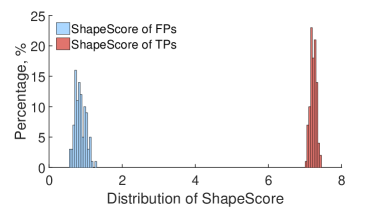
Figure 3. Histogram of the ShapeScore: The ShapeScore is computed for neighborhoods with 15,000 FVs each (experiment repeated 500 times to generate the histograms). Shape-based GD can reliably separate FPs and TPs through extracting information from the data that has been unutilized by an LD.

6.1. Can shape of alert-FVs identify malicious neighborhoods?

We first show that the shape of a neighborhood can easily distinguish between neighborhoods that are either 100% benign or 100% malicious. We quantify Shape-GD’s time to detection under real settings with a mix of both in subsequent sections.

Figure 3 shows that Shape-GD can indeed separate purely benign neighborhoods from purely malicious ones. To conduct this experiment, we construct purely benign and malicious neighborhoods with $\sim$15,000 benign or malicious FVs respectively (i.e., $|B|$ is 15,000). In Appendix C, we experimentally quantify the sensitivity of Shape-GD to the number of FVs in a neighborhood ($|B|$) and find that neighborhoods with more than 15,000 FVs lead to robust global classification.

For each neighborhood, we use the Random Forest LD to generate alert-FVs and use Shape-GD to compute the neighborhood’s ShapeScore using the alert-FVs from the neighborhood. In Figure 3, we plot histogram of ShapeScores for 500 benign and malicious FVs each – each point in the blue (or red) histogram represents the ShapeScore of a completely benign (or malicious) neighborhood. Recall that a small ShapeScore indicates the neighborhood’s statistical shape is similar to that of a benign one. The non-overlapping distributions separated by a large gap indicate that the shape of purely benign neighborhoods is very different from the shape of purely malicious neighborhoods.

Shape-GD detects anomalous neighborhoods by setting a threshold score based on the distribution of benign neighborhoods’ scores (Figure 3) – if an incoming neighborhood has a score above the threshold, Shape GD labels it as ‘malicious’, otherwise ‘benign’. We set the threshold score at 99-percentile (i.e. our expected global false positive rate is 1%) and the true positive rate is effectively 100% for this experiment. This shows that for homogeneous neighborhoods producing over 15K FVs within a neighborhood time window, Shape-GD can make robust predictions. The next question then is how well Shape-GD can do so when neighborhoods are partially infected – we evaluate this in the next section.

6.2. Time to detection using temporal neighborhoods

Temporal filtering creates a neighborhood using only the nodes that are active within a neighborhood time window (NTW). For example, a temporal neighborhood for the phishing scenario would include every email address that received an email within the last hour (1086 nodes in our experiments). Similarly, a waterhole attack scenario would include all client devices that accessed any server within the last NTW into one neighborhood ($\sim 17,000$ nodes on average in 30 seconds). This neighborhood filtering models a CIDS designed to detect malware whose infection exhibits temporal locality (and obviously does not detect attacks that target a few high-value nodes through temporally uncorrelated vectors).

Phishing and waterhole attacks operate at different time scales (and hence NTWs). Due to the long tail distribution of email ‘open’ times, the phishing NTW varies from 1–3 hours in our experiments. On the other hand, a popular waterhole server quickly infects a large number of clients within a short period of time – thus, we vary the waterhole NTW from 4 seconds up to 100 seconds.

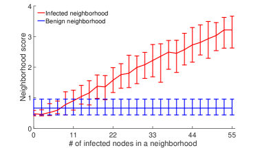
Figure 4. (Phishing attack: Time-based NF) Dynamics of an attack: While the portion of infected nodes in a neighborhood increases over time reaching 55 nodes out of 1086 on average, ShapeScore goes up showing that Shape GD becomes more confident in labeling neighborhoods as ‘malicious’. It starts detecting malware with at most 1% false positive rate when it compromises roughly 22 nodes. The neighborhood includes all 1086 nodes in a network and spans over 1 hour time interval.

Shape GD’s time to detection for one NTW. We fix NTWs (1 hour for phishing and 30 seconds for waterhole) and vary a parameter that represents a node’s likelihood of infection from 0% up to 100% – modeling whether a phished user clicks the malicious URL (phishing) or a drive-by exploit succeeeds in a waterhole attacks.

Figures 4 and 5 plot the neighborhood score v. the average number of infected nodes within benign (blue curve) and malicious (red curve) neighborhoods – the two extreme points on the X-axis corresponds to either none of the machines being infected (the left side of a figure) or the maximum possible number of machines being infected (the right side of the figure). In this experiment, phishing can infect up to 55 machines in the 1 hour NTW, while the waterhole server can infect almost 1250 nodes in the 30 seconds NTW. Every point on a line is the median neighborhood score from 10 experiments with whiskers set at 1%- and 99%- percentile scores.

When increasing the number of infected nodes in a neighborhood, as expected, the red curve larger deviates from the blue one. Therefore, Shape GD becomes more confident with labeling incoming partially infected neighborhoods as malicious. Shape GD starts reliably detecting malware very quickly – when only 22 nodes (phishing) and 200 nodes (waterhole) have been infected. We also experimented with other sizes of neighborhood window – the plots we obtained showed similar trends.

Shape GD’s sensitivity to NTW. We show that the size of a neighborhood is important for early detection – the minimum number of nodes that are infected before Shape GD raises an alert – in Figures 6 and 7. Varying the NTW essentially competes the rates at which both malicious and benign FVs accumulate – interestingly, we find that these relative rates are different for phishing and waterhole attacks and lead to different trends for detection performance v. NTW.

We vary the NTW from 1 hour to 3 hours for phishing and from 4 sec to 100 sec for waterhole and record the number of infected nodes when Shape GD can make robust predictions (i.e. less than 1% FP for almost 100% TP).

Increasing the NTW in the phishing experiment from 1 to 3 hours improves the Shape GD’s detection performance – at 17.08 infected nodes for a 3 hour NTW compared to 20.24 nodes for a 1 hour NTW. Detection improves slowly because while the infection rate slows down over time as fewer emails remain to be opened, the long tail distribution of email ‘open’ times causes most of the 17 victims to fall early in the NTW and accumulate sufficient malicious FVs to tip the overall neighborhood’s shape into malicious category.

In a waterhole scenario, the number of client devices active within a time window (and hence the false positive alert-FVs from the neighborhood) grows much faster than the malware can spread (even if we assume that every client that visits the waterhole server gets infected. Here, a large NTW aggregates many more benign (false positive) FVs from clients accessing non-compromised servers. Hence, in contrast to the phishing attack, increasing the NTW degrades time to detection. Shape GD works best with an NTW of 6 seconds – only 107.5 nodes on average become infected out of a possible $\sim$550,000 nodes. Note that a very small NTW (below 6 seconds) either does not accumulate enough FVs for analysis – if so, Shape GD outputs no results – or creates large variance in the shape of benign neighborhoods and abruptly degrades detection performance.

Note that a Shape GD requires a minimum number of FVs per neighborhood to make robust predictions – at least 15,000 FVs based on Appendix C – hence, the Shape GD has to set NTWs based on the rate of incoming requests and access frequency of a particular server. For example, if a server is not very popular and is likely to be compromised, the Shape GD could increase this server’s NTW to collect more FVs for its neighborhood.

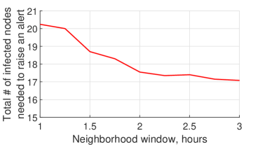
Figure 6. (Phishing attack: Time-based NF algorithm) Shape GD’s performance improves by 18.5% (20.24 and 17.08 infected nodes) when increasing the size of a neighborhood window from 1 hour to 3 hours.

6.3. Time to detection using structural information

Both phishing and waterhole attacks impose a logical structure on nodes (beyond their time of infection): phishing spreads malware through malicious email attachments or links while waterhole attacks infect only the clients that access a compromised server. This structure suggests that temporal neighborhoods can be further refined based on the sender/recipient-list of an email (e.g., grouping members of a mailing list into a neighborhood in the phishing scenario) or based on the specific server accessed by a client (i.e., grouping clients that visit a server into one neighborhood).

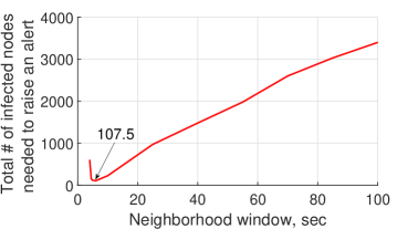
Figure 7. (Waterhole attack: Time-based NF) Shape GD’s performance deteriorates linearly when increasing the size of a neighborhood window from 6 sec to 100 sec.

To analyze the effect of such structural filtering on GD’s performance, we vary filtering from coarse- (no structural filtering, only time-based filtering) to fine-grained (aggregating alerts across each recipients’ list separately or across clients accessing each server separately) (Figures 8, 9). Specifically, the aggregation parameter changes from 50 recipients’ lists or servers down to 1. As before, we measure detection in terms of the minimum number of infected nodes that lead to raising a global alert. Also we consider three NTW values – 1-, 2-, and 3- hours long for phishing and 25-, 50-, and 100-sec long for waterhole.

Figure 8 shows that structural filtering improves detection of a phishing attack by $\sim 4x$ (difference between left and right end points of each curve) over temporal filtering – by filtering out alert-FVs from unrelated benign nodes that were active during the same NTW as infected nodes. Interestingly, the size of a neighborhood window does not considerably affect the detection when used along with the most fine-grained structural filtering (treating each recipients’ list individually) – 3-hour long NTWs results in only a $\sim 12\%$ decrease in the number of compromised nodes (i.e. time to detection). This shows that there is substantial signal that structural filtering can help extract from alert-FVs in smaller NTWs (and thus improve Shape GD’s time to detection).

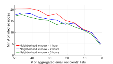
Figure 8. (Phishing attack) Comparing to pure time-based NF, structural filtering algorithm improves Shape GD’s performance by $\sim 4\times$ by taking into consideration logical structure of electronic communication (sender – receiver relation).

Structural filtering improves time to detect waterhole attacks as well – by 5.82x, 4.07x, and 3.75x for 25-, 50-, 100-sec long windows respectively. Interestingly, structural filtering requires Shape GD to use longer NTWs than before – small NTWs (such as 6 seconds from the last sub-section) no longer supply a sufficient number of alert-FVs for Shape GD to operate robustly. Even though structural filtering with a 25 second NTW improves detection by 5.82x over temporal filtering with 25 second NTWs, the number of infected nodes at detection time is 139.9 – higher than the 107 infected nodes for temporal filtering with a 6 second NTW (Figure 7). Temporal and structural filtering thus present different trade-offs between detection time and work performed by GD – their relative performance is affected by the rate at which true and false positive FVs are generated.

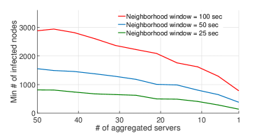
Figure 9. (Waterhole attack) Comparing to pure time-based NF, structural filtering algorithm improves Shape GD’s performance by $3.75\times$ – $5.8\times$ by aggregating alerts on a server basis.

6.4. Fragility of Count GD

A Count GD algorithm counts the number of alerts over a neighborhood and compares to a threshold to detect malware. This threshold scales linearly in the size of the neighborhood – we now experimentally quantify the error Count GD can tolerate in phishing (Figure 15) and waterhole (Figure 10) settings. Note that the error in estimating neighborhood size can be double sided – underestimates (negative error) can make neighborhoods look like alert hotspots and lead to false positives, while overestimates (positive error) can lead to missed detections (i.e., lower true positives).

We run Count GD in the same setting as Shape GD when evaluating time-based NF (Section 6.2) – 30-sec long neighborhood including 17,178 nodes (Figure 10) to model a waterhole attack and 1-hour long neighborhood time window (NTW) with 1086 nodes (Figure 15 in Appendix F) to model phishing. We vary infection probability (waterhole) and click rate in emails (phishing) such that the number of infected nodes in a neighborhood changes from 0 to 55 (phishing) and from 0 to 500 (waterhole) in four increments – note that in both scenarios, only a small fraction (5.5% and 2.9%) of nodes per neighborhood get infected in the worst case.

In this setting, recall that the Shape GD has a maximum global false positive rate of 1% and a true positive rate of 100% – and detects malware when only 22 (phishing) and 200 (waterhole) nodes are infected – for the same NTWs. When the same number of nodes are infected, and for a similar detection performance, our experiments show that the Count GD can only tolerate neighborhood size estimation errors within a very narrow range – [-2%, 6.3%] (phishing) and [-0.1%, 13.8%] (waterhole). A key takeaway here is that underestimating a neighborhood’s size makes Count GD extremely fragile (-2% in phishing and -0.1% for waterhole). On the other hand, overestimating neighborhood sizes decreases true positives, and this effect is catastrophic by the time the size estimates err by 17% (phishing) and 17.5% (waterhole).

We comment that this effect can be important in practice. Given the practical deployments where nodes get infected out of band (e.g., outside the corporate network), go out of range (with mobile devices), or with dynamically defined neighborhoods based on actions that can be missed (e.g. neighborhood defined by nodes that ‘open’ an email instead of only downloading it from a mail server), the tight margins on errors can render Count GD extremely unreliable. Even with sophisticated size estimation algorithms, recall that the underlying distributions that create these neighborhoods (email open times, number of clients per server, etc) have sub-exponential heavy tails (email-resp-dist, ) – such distributions typically result in poor parameter estimates due to lack of higher moments, and thus, poorer statistical concentrations of estimates about the true value (fkz11, ). Circling back, we see that by eliminating this size dependence compared to Count GD, our Shape GD provides a robust inference algorithm.

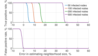
Figure 10. (Waterhole attack) An error in estimating neighborhood size dramatically affects Count GD’s performance. It can tolerate at most 0.1% underestimation errors and 13.8% overestimation errors to achieve comparable with Shape GD performance.

7. Conclusions

Building robust behavioral detectors is a long-standing problem. We observe that attacks on enterprise networks induce a low-dimensional structure on otherwise high-dimensional feature vectors, but this structure is hard to exploit because the correlations are hard to predict. By analyzing alert feature vectors instead of alerts and filtering the alert-FVs along neighborhood lines, we amplify the signal buried in correlated feature vectors, and then use the notion of statistical shape to classify neighborhoods without having to estimate the expected number of benign and false positive FVs per neighborhood. We note that both neighborhood-filtering and shape are complementary techniques that apply across a range of LDs or platforms – e.g., we have determined that Shape-GD also works well with n-grams based LDs (instead of histograms) and on the Android platform (in addition to Windows).

Our methodology composes the traditional host-level malware analysis methodology with trace-based simulations from real web services (to overcome the lack of joint LD-GD datasets), and allow us to run sensitivity analyses that will be precluded by using an actual enterprise trace. We find that Shape-GD reduces the number of FPs reported to deeper analyses by $\sim$100$\times$ and $\sim$200$\times$ when employing time-based filtering only (for phishing and waterhole scenarios respectively), while structural filtering reduces alert-FVs to $\sim$1000$\times$ and $\sim$830$\times$ (Appendix E). Neighborhoods and their shape thus serve as a new and effective lens for dimensionality reduction and significantly improve false positive rates of state-of-the-art behavioral analyses. For example, LDs can operate at a higher false positive rate in order to reduce false negatives and improve computation efficiency.

Appendix A How accurate is clustering for global malware detection?

While Count GD is fragile, clustering GDs are inaccurate in the early stages of infection. This is why prior work (beehive2013, ) uses clustering to (offline) identify high-priority incidents from security logs for human analysis (instead of as an always-on GD) – this use case is complementary to an always-on global detector. We quantify a recent clustering GD’s (beehive2013, ) detection rate on our data set.

First, we reduce dimensionality of 390-dimensional FVs by projecting them on the top 10 PCA components, which retain 95.72% of the data variance. Second, we use an adaptation of the K-means clustering algorithm that does not require specifying the number of clusters in advance (beehive2013, ; Seurat2004, ; kaufman_clustering, ). Specifically, the algorithm consists of the following three steps: (1) select a vector at random as the first centroid and assign all vectors to this cluster; (2) find a vector furthest away from its centroid (following Beehive (beehive2013, ), we use L1 distance) and make it a center of a new cluster, and reassign every vector to the cluster with the closest centroid; and (3) repeat step 2 until no vector is further away from its centroid than half of the average inter-cluster distance.

The evaluation settings of the clustering algorithm match exactly the settings where Shape GD detects infected neighborhoods with 99% confidence. Specifically, the algorithm clusters the data that we collected in a 17,178-node neighborhood under a waterhole attack within 30 seconds and the data that we collected over an hour-long session across 1086 nodes in a medium size corporate network under a phishing attack (Section 5.3). As we have already demonstrated (Section 6.2), Shape GD starts detecting malware when 107 (waterhole attack) and 22 (phishing attack) nodes get compromised (as in experiments for Figures 4 and 5).

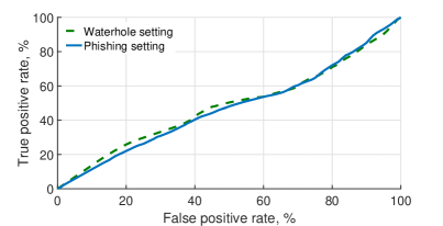
Figure 11. (ROC curve) True positive v. False positive curve shows detection accuracy of the clustering-based malware detector (beehive2013, ). Its Area Under the Curve (AUC) parameter averaged for 10 runs reaches only 48.3% and 47.4% in the case of waterhole and phishing attacks respectively; such low AUC value makes it unusable as a global detector.

Clustering does not fare well, and results look very similar for both waterhole and phishing experiments. The clustering algorithm partitions waterhole data set into 30 clusters. We observe three large clusters that aggregate most of the benign FVs. However, the algorithm fails to find small ’outlying’ clusters consisting of predominantly malicious data. As for the phishing experiment, we observe a similar picture: the algorithm forms slightly higher number of clusters – 33 rather than 30 – and it identifies 4 densely populated clusters. In both cases each cluster heavily mixes benign and malicious data, hence the clustering approach suffers from poor discriminative ability, i.e. it is unable to separate malicious and benign samples.

Note the clustering algorithm enforces explicit ordering across the clusters. That is, the algorithm forms a new cluster around an FV that is furthest away from its cluster centroid. Thus, earlier a cluster is created, the more suspicious it is. By design of the clustering algorithm, the clusters are subject to a deeper analysis in order of their suspiciousness. Such an inherent ordering allows us to build a receiver operating curve (Figure 11) and compute a typical metric for a binary classifier – Area Under the Curve (AUC) by averaging across 10 runs. The AUC reaches only 48.3% and 47.4% for waterhole and phishing experiments respectively.

This experiment illustrates the failure of the traditional recipe of dimensionality reduction plus clustering. There is a fundamental reason for this – the neighborhoods we seek to detect are small compared to the total number of nodes in the system. Optimization-based algorithms that exploit density, including K-Means and related algorithms, fail to detect small clusters in high dimensions, even under dimensionality reduction. The reason is that the dimensionality reduction is either explicitly random (e.g., as in Johnson-Lindenstrauss type approaches), or, if data-dependent (like PCA), it is effectively independent of small clusters, as these represent very little of the energy (the variance) of the overall data. Spectral clustering style algorithms (spectral_clustering_tutorial_2007, ; on_spectral_clustering_ng_01, ; evolutionary_spectral_clustering, ) are also notoriously unable to deal with highly unbalanced sized clusters, and in particular, are unable to find small clusters.

Shape GD also reduces dimensionality but does so after neighborhood filtering. This amplifies the impact of small neighborhoods. The combination of dimensionality reduction, small-neighborhood-amplification, and then aggregation represents a novel approach to this detection problem, and our experiments validate this intuition.

Appendix B Local Detectors

Our first step is to establish a good local detector (LD) for desktop systems running Windows OS. In particular, we choose system call based LDs since the system call interface has visibility into an app’s intercation with core OS components – file system, Windows registry, network – and can thus capture signals relevant to malware executions.

We experiment with an extensive set of system-call LDs – our takeaway is that even the best LD we could construct operates at a true- and false-positive ratio of 92.4%:6% and is not deployable by itself (i.e., will create $\sim$30 false positives every 10 minutes without a GD).

Each LD comprises of a feature extraction (FE) algorithm and a machine learning (ML) classifier. Our FE algorithm partitions the time-series of system calls into 1-sec chunks and represents each chunk as a histogram (where each bin contains frequency of a particular system call). Then it projects all feature vectors onto 10-dimensional subspace spanned by top 10 principal components generated by PCA algorithm. We choose ML classifiers (used throughout prior work because these are computationally efficient to train) such as SVMs, random forest, k-Nearest Neighbors, etc, and do not include complex alternatives such as artificial neural networks or deep learning algorithms. We also deliberately avoid handcrafted ML algorithms and hardcoded detection rules.

Figure 12 plots the true positive v. false positive rates (i.e. the ROC curves) of the seven ML algorithms we evaluate. The area under the ROC curve (AUC) is a quantitative measure of LD’s performance: the larger the AUC, the more accurate the detector. We specifically experiment with seven state-of-the-art ML algorithms: random forest, 2-class SVM, kNN, decision trees, naive Bayes, and their ensemble versions – boosted decision trees with AdaBoost algorithm and Random SubSpace ensemble of kNN classifiers (Figure 12). We also evaluated 1-class SVM as an anomaly detector – however, it yielded an extremely high FP rate and we exclude it from further discussion. Overall, the random forest classifier worked best – it has the highest AUC and we pick an operating point of 92.4% true positives at a false positive rate of 6%.

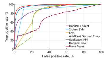
Figure 12. (ROC curves) True positive v. False positive curves shows detection accuracy of seven local detectors. Random Forest outperforms all others; but has unacceptably high false positive rate (above 10%) if one wants to achieve at least 95% true positive rate.

Appendix C How many FVs does Shape GD need to make robust predictions?

The number of FVs per neighborhood required by Shape-GD to make a robust prediction is a crucial parameter. With too few FVs produced by a neighborhood, benign neighborhoods’ ShapeScore will have high variance (i.e. benign distribution in Figure 3 becomes wide and the gap between two distributions shrinks), leading to global false positives and negatives. On the other hand, if neighborhoods are large, their ShapeScores will be dominated by the large number of benign FVs and thus lead to missed alerts (false negatives) especially in the early stages of infection. Further, the number of alert-FVs generated by a neighborhood in a deployed Shape-GD need to be comparable to or larger than those used in training – hence, we want to determine the smallest number of FVs Shape-GD needs to make a robust prediction.

Figure 13 shows the sensitivity of Shape-GD to neighborhood size (i.e., the number of FVs generated by nodes in a neighborhood during training stage). We vary the number of FVs that a neighborhood generates from 3,000 up to 30,000 FVs and average the results of 10 experiments. We present two metrics in Figure 13 – the red curve plots the inter-class distance (between histograms of benign and malicious neighborhoods from Figure 3), and the blue curve plots intra-class distance (i.e. the width of the benign histogram). Figure 13 shows that the red inter-class distance increases (and blue intra-class variance decreases) quickly as neighborhood size increases, and both curves flatten out once the neighborhoods start generating more than 15,000 FVs.

This shows that (for our Windows programs dataset) neighborhoods generating 15,000 FVs or more are a good choice to train Shape GD because purely malicious or benign distributions stabilize at this size. In real scenarios with mixtures of mostly benign and a few malicious neighborhoods, the number of FVs will have to be scaled up depending upon the timescale of attacks (hours for phishing v. seconds for waterhole) and the number of nodes affected by an attack (tens of nodes in enterprise email networks v. thousands in a broader waterhole attack on the enterprise). In the phishing and waterhole attack case studies in the paper, we use neighborhoods of 1,086 and $\sim$17,000 nodes that produce 15k FVs and 100k FVs respectively.

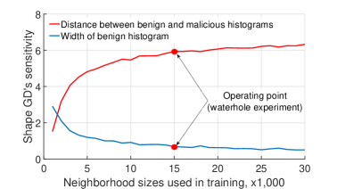
Figure 13. Analysis of ShapeScore histogram parameters when changing neighborhood size. The curves flatten out on the right side from the operating point.

Appendix D Computation and Communication Costs of Shape-GD

Local detectors. Generating a single FV, which is a 1-sec histogram of system calls, on a local host is equivalent to performing 2,500 (system call frequency) direct table lookups on average and incrementing corresponding counters. Projection on a PCA basis requires computing 10 dot products. Finally, running an LD, which is Random Forest in our case, results in performing 330 scalar comparisons on average. At 1 second per FV, the overheads of such an LD are negligible.

Data transfer. Each FV is composed of 10 floating point numbers (40 bytes total if assuming single precision format). In the phishing experiment 1086 hosts transfer (in aggregate) $\sim 40KB/sec$; data transfer rate in waterhole setting is a little bit higher: $\sim 4,450$ hosts transfer (in aggregate) $\sim 174KB/sec$. In both cases we assume Shape GD using pure time-based filtering with 1 hour and 6 sec neighborhood time windows respectively.

If Shape GD employs structural filtering on top of the time-based one, then data transfer depends on the number of emails floating in a network or on the number of servers. In both cases, data transfer scales linearly with the number of emails and servers. When applying the most fine-grained structural filtering in our experiments, the nodes susceptible to phishing attacks transfer $\sim 4KB/sec$ per email and the nodes susceptible to waterhole attacks send $\sim 40KB/sec$ per server when using 1 hour and 25 sec neighborhood windows respectively.

Server computations. After receiving a batch of alert-FVs, Shape GD performs lightweight computations. Overhead of binning scales linearly with the number of alert-FVs in a batch; each binning operation is a direct table lookup together with counter increment. Calculating ShapeScore, which is Wasserstein distance, results in a sequence of addition operations, whose total number is equal to the dimensionality of FVs, which is 10, multiplied by the number of bins, which is 50. To summarize, Shape GD’s computational requirements are fairly light-weight.

Appendix E Discussion

Global FPs vs LD FPs. As remarked in the Introduction, an FP of 1% at the global level means that we will see one alert every 100 - 300 hours (for the phishing scenario) and 100 seconds (for waterhole scenario the neighborhood time window slides by 1 second). This reduces work to be performed by the deeper, second-level analysis considerably.

Specifically, LDs operating at 6% false positive rate generate 23.5M – 70M FPs within 100–300 hours time interval in a network of 1086 nodes (phishing) and 300K alerts within every 100 sec interval where neighborhoods include $\sim$50K nodes on average (waterhole). Shape GD filters these alerts. When using 1–3 hours (phishing) and 6 sec (waterhole) time-based neighborhood filtering, Shape GD will report to a system running a deeper analysis approximately 234.5K – 703.7K FPs raised by LDs (phishing) and approximately 1.4K FPs (waterhole). Adding structural filtering brings these numbers down to 21.6K – 64.8K FPs (phishing) and 360 FPs (waterhole).

Compared to a neighborhood of LDs, Shape GD thus reduces the number of FPs reported to deeper analyses by $\sim$100$\times$ and $\sim$200$\times$ when employing time-based filtering only (for phishing and waterhole scenarios respectively), while structural filtering reduces alert-FVs for deeper analysis to $\sim$1000$\times$ and $\sim$830$\times$. In both scenarios, analysts can choose to reduce number of alert-FVs to be analyzed by sliding neighborhood windows by a larger interval; however, this will increase the time to detect malware infection.

Shape property across LDs and platforms. Shape-GD relies on conditional separability of FPs and TPs, and we use only one LD type for evaluation – a system call histogram-based LD. However, we have experimentally determined that FPs and TPs are separable for other LD types as well – an n-gram-based LD (mutant_x, ) and an LD that uses VirusTotal (virustotal, ) reports for malware detection (vt_report_classification, ). Further, we can classify malicious neighborhoods on the Android platform – using malware binaries obtained from the NCSU dataset and contagio dump website, and using benign applications that we drive using real human user input – in addition to the Windows setup that we describe here. We have left out the details due to lack of space but can produce an anonymous report if requested.

Though the local detectors we built have a 6% FP rate, Shape-GD can work well work with better LDs. Shape-GD only requires LD’s FPs and TPs to be separable and to be able to aggregate enough alert-FVs across the nodes within a neighborhood. We deliberately do not consider rule-based LDs that are commonly used within enterprise networks because, even though their FP rate is very low, they suffer from a high false negative rate, and they can be easily evaded with simple malware transformations.

Performance Overheads. Recall that Shape GD requires only alert FVs – this leads to a two-fold dimensionality reduction when sending data from individual LDs to the GD. First, the FVs are low-dimensional (here, 10-dimensional vectors). Second, only alert FVs are needed – this leads to a 16-fold reduction in data (roughly only 6% of the FVs lead to alerts). Further, the Shape GD is a batch processing algorithm, thus, the individual nodes can batch their data at coarse time-scales (e.g. once every NTW) and send the data to the Shape GD. Finally, it does not matter even if some batches are lost/missed; recall that the Shape GD is robust to precisely this type of noise. Appendix A discusses overheads in more depth but the key takeaway is that Shape GD has low overheads – each LD can use simple dot products and scalar comparisons to implement PCA and Random Forests, the total incoming bandwidth to the Shape GD server ranges from 40KBps to 174KBps for phishing and waterhole respectively, and the server only needs to bin data (into 50 bins) and compute Wasserstein distance (add 10 counters in each bin).

Detailed Shape-GD Pipeline. As an extension to the description in Section 4, Figure 14 shows the detailed machine learning pipeline for extracting one neighborhood’s shape into a ShapeScore.

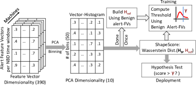
Figure 14. (Overview) Shape-GD machine learning pipeline.

Appendix F How fragile is Count GD to errors in estimating neighborhood size? (Phishing)

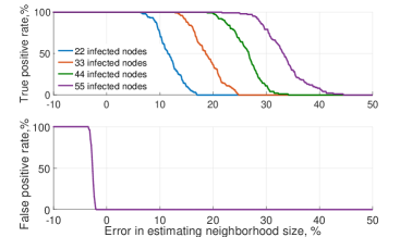
Figure 15. (Phishing attack) An error in estimating neighborhood size dramatically affects Count GD’s performance. It can tolerate at most 2% underestimation errors and 6.3% overestimation errors to achieve comparable with Shape GD performance.

Due to space considerations, we have placed the results for Count GD’s fragility to mis-estimated neighborhood sizes in the appendix in Figure 15. The key trends are similar to waterhole attack presented in the main paper – even a slight under- or over-estimate of dynamic neighborhoods’ sizes can yield completely inaccurate results.

References

- (1) http://www.fraudwatchinternational.com/phishing-alerts.
- (2) Advanced malware protection (amp). http://www.cisco.com/c/en/us/products/security/advanced-malware-protection/index.html.
- (3) Advanced malware protection and detection (ampd). https://www.secureworks.com/capabilities/managed-security/network-security/advanced-malware-protection.
- (4) Attack graphs: visualizing 200m alerts a day. http://on-demand.gputechconf.com/gtc/2016/presentation/s6114-leo-meyerovich-attack-graphs-visualizing-alerts.pdf.
- (5) Data binning. https://en.wikipedia.org/wiki/Histogram.
- (6) Enron email dataset. https://www.cs.cmu.edu/~./enron.
- (7) G4 - yahoo! network flows data. https://webscope.sandbox.yahoo.com.
- (8) Graphistry. https://www.iqt.org/graphistry.
- (9) Grr rapid response: remote live forensics for incident response. https://github.com/google/grr.
- (10) Hone tool. https://github.com/pmoody-/Linux-Sensor.
- (11) Kaspersky security bulletin 2015. https://securelist.com/files/2015/12/Kaspersky-Security-Bulletin-2015_FINAL_EN.pdf.
- (12) Lastline: Defeat advanced malware before it infiltrates your network. https://www.lastline.com.
- (13) osquery – performant endpoint visibility. https://osquery.io/.
- (14) Securerank algorithm. https://blog.opendns.com/2013/03/28/secure-rank-a-large-scale-discovery-algorithm-for-predictive-detection.
- (15) Statement regarding cyber attack against anthem. http://www.sophos.com/en-us/threat-center/mobile-security-threat-report.aspx.
- (16) Symantec intelligence report. https://www.symantec.com/content/en/us/enterprise/other_resources/b-intelligence-report-01-2015-en-us.pdf.
- (17) Symantec report on black vine espionage group. http://www.symantec.com/content/en/us/enterprise/media/security_response/whitepapers/the-black-vine-cyberespionage-group.pdf.
- (18) Virustotal – free online virus, malware and url scanner. https://www.virustotal.com.
- (19) Wasserstein metric. https://en.wikipedia.org/wiki/Wasserstein_metric.
- (20) Why watering hole attacks work. https://threatpost.com/why-watering-hole-attacks-work-032013/77647.
- (21) Bailey, M., Oberheide, J., Andersen, J., Mao, Z., Jahanian, F., and Nazario, J. Automated classification and analysis of internet malware. In Recent Advances in Intrusion Detection. 2007.
- (22) Benamou, J., and Brenier, Y. Mixed l2-wasserstein optimal mapping between prescribed density functions. Journal of Optimization Theory and Applications (2001).
- (23) Bethencourt, J., Franklin, J., and Vernon, M. Mapping internet sensors with probe response attacks. In Proceedings of the 14th USENIX Security Symposium (2005).
- (24) Burguera, I., Zurutuza, U., and Nadjm-Tehrani, S. Crowdroid: Behavior-based malware detection system for android. In Proceedings of the 1st ACM Workshop on Security and Privacy in Smartphones and Mobile Devices (2011), SPSM.
- (25) Canali, D., Lanzi, A., Balzarotti, D., Kruegel, C., Christodorescu, M., and Kirda, E. A quantitative study of accuracy in system call-based malware detection. In Proceedings of the 2012 International Symposium on Software Testing and Analysis (2012), ISSTA 2012.
- (26) Chi, Y., Song, X., Zhou, D., Hino, K., and Tseng, B. L. Evolutionary spectral clustering by incorporating temporal smoothness. In Proceedings of the 13th ACM SIGKDD International Conference on Knowledge Discovery and Data Mining (2007), KDD ’07.
- (27) Christodorescu, M., Jha, S., and Kruegel, C. Mining specifications of malicious behavior. In Proceedings of the 1st India Software Engineering Conference (2008), ISEC.
- (28) Christodorescu, M., Jha, S., Seshia, S. A., Song, D., and Bryant, R. E. Semantics-aware malware detection. In Proceedings of the 2005 IEEE Symposium on Security and Privacy (2005).
- (29) Clark, S. S., Ransford, B., Rahmati, A., Guineau, S., Sorber, J., Xu, W., and Fu, K. WattsUpDoc: Power side channels to nonintrusively discover untargeted malware on embedded medical devices. In USENIX Workshop on Health Information Technologies (2013).
- (30) Dash, D., Kveton, B., Agosta, J. M., Schooler, E., Chandrashekar, J., Bachrach, A., and Newman, A. When gossip is good: Distributed probabilistic inference for detection of slow network intrusions. In Proceedings of the 21st National Conference on Artificial Intelligence (2006).
- (31) Demme, J., Maycock, M., Schmitz, J., Tang, A., Waksman, A., Sethumadhavan, S., and Stolfo, S. On the feasibility of online malware detection with performance counters. In Proceedings of the 40th Annual International Symposium on Computer Architecture (2013).
- (32) Donoho, D. L., and Huber, P. J. The notion of breakdown point. A festschrift for Erich L. Lehmann 157184 (1983).
- (33) Fink, G. A., Duggirala, V., Correa, R., and North, C. Bridging the host-network divide: Survey, taxonomy, and solution. In Proceedings of the 20th Conference on Large Installation System Administration (Berkeley, CA, USA, 2006), LISA ’06, USENIX Association, pp. 20–20.
- (34) Forrest, S., Hofmeyr, S., Somayaji, A., and Longstaff, T. A sense of self for unix processes. In Security and Privacy, 1996. Proceedings., IEEE Symposium on (1996).
- (35) Foss, S., Korshunov, D., and Zachary, S. An introduction to heavy-tailed and subexponential distributions, 2009. Springer Series in Operations Research and Financial Engineering.
- (36) Fredrikson, M., Jha, S., Christodorescu, M., Sailer, R., and Yan, X. Synthesizing near-optimal malware specifications from suspicious behaviors. In IEEE Symposium on Security and Privacy (2010).
- (37) Gu, G., Porras, P., Yegneswaran, V., Fong, M., and Lee, W. Bothunter: Detecting malware infection through ids-driven dialog correlation. In Proceedings of 16th USENIX Security Symposium (2007).
- (38) Gu, G., Zhang, J., and Lee, W. Botsniffer: Detecting botnet command and control channels in network traffic. In Presented at the 16th Annual Network & Distributed System Security Symposium (2008), NDSS.
- (39) Handley, M., Paxson, V., and Kreibich, C. Network intrusion detection: Evasion, traffic normalization, and end-to-end protocol semantics. In Proceedings of the 10th Conference on USENIX Security Symposium - Volume 10 (Berkeley, CA, USA, 2001), SSYM’01, USENIX Association.
- (40) Hanna, S., Huang, L., Wu, E., Li, S., Chen, C., and Song, D. Juxtapp: A scalable system for detecting code reuse among android applications. In Detection of Intrusions and Malware, and Vulnerability Assessment. 2013.
- (41) Hu, X., Bhatkar, S., Griffin, K., and Shin, K. G. Mutantx-s: Scalable malware clustering based on static features. In Proceedings of the 2013 USENIX Conference on Annual Technical Conference (Berkeley, CA, USA, 2013), USENIX ATC’13, USENIX Association, pp. 187–198.
- (42) Huber, P. J. Robust statistics. Springer, 2011.
- (43) Kaufman, L., and Rousseeuw, P. J. Finding Groups in Data: An Introduction to Cluster Analysis. John Wiley, 1990.
- (44) Khasawneh, K. N., Ozsoy, M., Donovick, C., Abu-Ghazaleh, N., and Ponomarev, D. Ensemble learning for low-level hardware-supported malware detection. In Research in Attacks, Intrusions, and Defenses. Springer International Publishing, 2015, pp. 3–25.
- (45) Kirat, D., Vigna, G., and Kruegel, C. Barecloud: Bare-metal analysis-based evasive malware detection. In Proceedings of the 23rd USENIX Conference on Security Symposium (2014).
- (46) Kolbitsch, C., Comparetti, P. M., Kruegel, C., Kirda, E., Zhou, X., and Wang, X. Effective and efficient malware detection at the end host. In Proceedings of the 18th Conference on USENIX Security Symposium (2009).
- (47) Kooti, F., Aiello, L. M., Grbovic, M., Lerman, K., and Mantrach, A. Evolution of conversations in the age of email overload. In Proceedings of 24th International World Wide Web Conferenced (WWW) (2015).
- (48) Krüegel, C., Toth, T., and Kerer, C. Decentralized event correlation for intrusion detection. In Proceedings of the 4th International Conference Seoul on Information Security and Cryptology (2002), ICISC ’01, Springer-Verlag.
- (49) Kwon, B. J., Mondal, J., Jang, J., Bilge, L., and Dumitras, T. The dropper effect: Insights into malware distribution with downloader graph analytics. In Proceedings of the 22Nd ACM SIGSAC Conference on Computer and Communications Security (New York, NY, USA, 2015), CCS ’15, ACM, pp. 1118–1129.
- (50) Locasto, M., Parekh, J., Keromytis, A., and Stolfo, S. Towards collaborative security and p2p intrusion detection. In Information Assurance Workshop, IAW (2005).
- (51) Mihai Christodorescu, S. J. Static analysis of executables to detect malicious patterns. Tech. rep., The University of Wisconsin, Madison, 2006.
- (52) Miller, B., Kantchelian, A., Tschantz, M. C., Afroz, S., Bachwani, R., Faizullabhoy, R., Huang, L., Shankar, V., Wu, T., Yiu, G., Joseph, A. D., and Tygar, J. D. Reviewer integration and performance measurement for malware detection. In Proceedings of the 13th International Conference on Detection of Intrusions and Malware, and Vulnerability Assessment - Volume 9721 (New York, NY, USA, 2016), DIMVA 2016, Springer-Verlag New York, Inc., pp. 122–141.
- (53) Nagaraja, S., Mittal, P., Hong, C.-Y., Caesar, M., and Borisov, N. Botgrep: Finding p2p bots with structured graph analysis. In Proceedings of the 19th USENIX Conference on Security (Berkeley, CA, USA, 2010), USENIX Security’10, USENIX Association, pp. 7–7.
- (54) Ng, A. Y., Jordan, M. I., and Weiss, Y. On spectral clustering: Analysis and an algorithm. In ADVANCES IN NEURAL INFORMATION PROCESSING SYSTEMS (2001).
- (55) Oprea, A., Li, Z., Yen, T.-F., Chin, S. H., and Alrwais, S. Detection of early-stage enterprise infection by mining large-scale log data. In Proceedings of the 2015 45th Annual IEEE/IFIP International Conference on Dependable Systems and Networks (Washington, DC, USA, 2015), DSN ’15, IEEE Computer Society, pp. 45–56.
- (56) Papernot, N., McDaniel, P., Goodfellow, I., Jha, S., Celik, Z. B., and Swami, A. Practical black-box attacks against machine learning. In Proceedings of the 2017 ACM on Asia Conference on Computer and Communications Security (New York, NY, USA, 2017), ASIA CCS ’17, ACM, pp. 506–519.
- (57) Paxson, V. Bro: A system for detecting network intruders in real-time. Comput. Netw. 31, 23-24 (1999), 2435–2463.
- (58) Provos, N., Mavrommatis, P., Rajab, M. A., and Monrose, F. All your iframes point to us. In Proceedings of the 17th Conference on Security Symposium (Berkeley, CA, USA, 2008), SS’08, USENIX Association, pp. 1–15.
- (59) Robertson, W., Maggi, F., Kruegel, C., and Vigna, G. Effective anomaly detection with scarce training data. In Proceedings of the Network and Distributed System Security Symposium (NDSS) (2010).
- (60) Shin, S., Xu, Z., and Gu, G. EFFORT: Efficient and Effective Bot Malware Detection. In Proceedings of the 31th Annual IEEE Conference on Computer Communications (INFOCOM’12) Mini-Conference (March 2012).
- (61) Shinoda, Y., Ikai, K., and Itoh, M. Vulnerabilities of passive internet threat monitors. In Proceedings of the 14th Conference on USENIX Security Symposium (2005).
- (62) Shmatikov, V., and Wang, M.-H. Security against probe-response attacks in collaborative intrusion detection. In the Workshop on Large Scale Attack Defense (2007).
- (63) Sommer, R., and Paxson, V. Outside the closed world: On using machine learning for network intrusion detection. In the IEEE Symposium on Security and Privacy (2010).
- (64) Šrndić, N., and Laskov, P. Practical evasion of a learning-based classifier: A case study. In the IEEE Symposium on Security and Privacy (2014).
- (65) Tang, A., Sethumadhavan, S., and Stolfo, S. Unsupervised anomaly-based malware detection using hardware features. In Research in Attacks, Intrusions and Defenses. 2014.
- (66) Vallender, S. Calculation of the wasserstein distance between probability distributions on the line. Theory of Probability & Its Applications 18, 4 (1974), 784–786.
- (67) Vlachos, V., Androutsellis-Theotokis, S., and Spinellis, D. Security applications of peer-to-peer networks. Comput. Netw. 45, 2 (2004).
- (68) von Luxburg, U. A tutorial on spectral clustering. Statistics and Computing (2007).
- (69) Wagner, D., and Soto, P. Mimicry attacks on host-based intrusion detection systems. In the ACM Conference on Computer and Communications Security (2002).
- (70) Xie, Y., Kim, H., O’Hallaron, D. R., Reiter, M. K., and Zhang, H. Seurat: A pointillist approach to anomaly detection. In Recent Advances in Intrusion Detection (2004).
- (71) Xu, H., Caramanis, C., and Mannor, S. Outlier-robust pca: the high-dimensional case. IEEE transactions on information theory 59, 1 (2013), 546–572.
- (72) Xu, W., Qi, Y., and Evans, D. Automatically evading classifiers: A case study on pdf malware classifiers. In Network and Distributed Systems Symposium (2016).
- (73) Yen, T.-F., Oprea, A., Onarlioglu, K., Leetham, T., Robertson, W., Juels, A., and Kirda, E. Beehive: Large-scale log analysis for detecting suspicious activity in enterprise networks. In Proceedings of the 29th Annual Computer Security Applications Conference (2013), ACSAC ’13, ACM, pp. 199–208.
- (74) Zhang, Z., Li, J., Manikopoulos, C. N., Jorgenson, J., and Ucles, J. Hide: a hierarchical network intrusion detection system using statistical preprocessing and neural network classification. In the IEEE Workshop on Information Assurance and Security (2001).
- (75) Zhao, Y., Xie, Y., Yu, F., Ke, Q., Yu, Y., Chen, Y., and Gillum, E. Botgraph: Large scale spamming botnet detection. In Proceedings of the 6th USENIX Symposium on Networked Systems Design and Implementation (Berkeley, CA, USA, 2009), NSDI’09, USENIX Association, pp. 321–334.