A combination chaotic system and application in color image encryption

Abstract

In this paper, by using Logistic, Sine and Tent systems we define a combination chaotic system. Some properties of the chaotic system are studied by using figures and numerical results. A color image encryption algorithm is introduced based on new chaotic system. Also this encryption algorithm can be used for gray scale or binary images. The experimental results of the encryption algorithm show that the encryption algorithm is secure and practical.

^aDepartment of Mathematics, University of Mohaghegh Ardabili, 56199-11367 Ardabil, Iran.

Keywords: Encryption; Color image; Chaotic system; Cyclic shift.

1 Introduction

Image plays an important role in the data transfer. With rapid development network communication, image security has become increasingly important. The first step in chaotic encryption was introduced by Matters [1]. In recent years, much attention has been given in the literature to the development, analysis and implementation of chaotic system for the image and the data encryption; see, for example, [2, 3, 4, 5, 6]. Chaos maps as Logistic map, Sine map and Tent map are used in image encryption algorithm because chaotic maps have high sensitivity to their initial values and control parameters [7, 8]. Logistic, Sine and Tent maps have some disadvantages. These maps for some values of $r$ have chaotic behavior. Also these maps have non-uniform distribution over output. Many methods have been proposed to solve these problems, for example see [9]. To overcome these problems, in this paper by using different functions as $\sin(x),\cos(x),\ldots$, we combine Logistic (or Sine) map and Tent map then by using this combination the different chaotic systems can be found. In the next step by using combination map, XOR operation and circ shift the color image encryption algorithm is introduced. In this encryption algorithm in the first step, color image is divided into twelve parts and then by using combination map the encryption process for each of the parts is done, in the last step, we combine parts and then the encryption process combination image is repeated.

The organization of this paper is as follows: In Section 2, Logistic-Tent combination map is explained. In Section 3, we present the color image encryption algorithm. Simulation results and security analysis are given in Section 4. A summary is given at the end of the paper in Section 5.

2 A combination chaotic system

In this section, we describe our combination of chaotic systems. Logistic, Sine and Tent maps are defined as follows

$$x_{n+1}=L(r,x_{n}):=rx_{n}(1-x_{n}),$$ (2.1)

$$x_{n+1}=S(r,x_{n}):=r\sin(\pi x_{n})/4,$$ (2.2)

$$x_{n+1}=T(r,x_{n}):=\left\{\begin{array}[]{ll}rx_{n}/2,&when~{}x_{n}<0.5,\\ \\ r(1-x_{n})/2,&when~{}x_{n}\geq 0.5.\\ \end{array}\right.$$ (2.6)

where parameter $r\in(0,4]$. It is known that the Logistic system (Sine or Tent system) for some values of $r\in(0,4]$ has chaotic behavior. Fig 2 and Fig 4 show that the Logistic system for $r=2$ has not chaotic behavior. To overcome the above problem, the combination of chaotic system as Logistic Tent system (LTS) introduced in [9]. Histogram of the Logistic Tent system is showed in Fig 3. Chaotic range is not limited for the Logistic Tent system but from Fig 3 we can see that the histogram of the Logistic Tent system is not flat enough. Non-uniform distribution over output series leads to weakness in the statistical attack. For solving this problem we add weights and functions in the Logistic Tent system or the Sine Tent system as follows

$$x_{n+1}=G_{r}(x_{n}):=$$

$$\left\{\begin{array}[]{ll}\omega_{1}f_{1}\circ F(r,x_{n})+\alpha_{1}g_{1}(rx_{n})+\xi_{1}\frac{(\beta_{1}-r)x_{n}}{2}~{}mod~{}1,&when~{}x_{n}<0.5,\\ \\ \omega_{2}f_{2}\circ F(r,x_{n})+\alpha_{2}g_{2}(rx_{n})+\xi_{2}\frac{(\beta_{2}-r)(1-x_{n})}{2}~{}mod~{}1,&when~{}x_{n}\geq 0.5,\\ \end{array}\right.$$ (2.10)

where $F(r,x_{n})$ is Logistic or Sine map. In (2), $f_{i}(x)$ and $g_{i}(x)~{}(i=1,2)$ can be considered as $ax,\sin(ax),$ $\cos(ax),\tan(ax),$ $\cot(ax),\exp(ax),\log(ax)$ (where $a$ is real constant) and any other appropriate function. Also in the above formula, $\omega_{i},$ $\alpha_{i},\xi_{i}$ and $\beta_{i}~{}(i=1,2)$ are real numbers and parameter $r\in(0,4]$. In next step to investigate the properties of the new system, we consider the following cases

• i: $2\omega_{1}=\omega_{2}=20,-\alpha_{1}=\alpha_{2}=-2,2\xi_{1}=\xi_{2}=4,\beta_{1}=4,$ $\beta_{2}=-20,f_{1}(x)=\sin(x),f_{2}(x)=\exp(x),g_{1}(t)=\cot(x),g_{2}=\cos(\pi x),F(r,x_{n})=L(r,x_{n})$.
  

• ii: $\omega_{1}=\omega_{2}=20,-\alpha_{1}=\alpha_{2}=0,2\xi_{1}=\xi_{2}=1,\beta_{1}=\beta_{2}=80,$ $f_{1}(x)=\sin(x),f_{2}(x)=\exp(x),F(r,x_{n})=L(r,x_{n})$.
  

• iii: $\omega_{1}=\omega_{2}=1,\alpha_{1}=\alpha_{2}=1,\xi_{1}=7,\xi_{2}=15,\beta_{1}=2\beta_{2}=40,$ $f_{1}(x)=\cos(x),f_{2}(x)=\tan(x),g_{1}(x)=\tan(x),g_{2}(x)=x,F(r,x_{n})=S(r,x_{n})$.

For discrete time system as (2), the Lyapunov exponent for an orbit starting with $x_{0}$ is defined as follows

$$LE(x_{0},r):=\lim_{n\rightarrow\infty}\frac{1}{n}\sum^{n-1}_{i=0}\ln|G_{r}^{\prime}(x_{i})|.$$ (2.11)

The degree of ”sensitivity to initial conditions” can be measured by using the Lyapunov exponent. In [10] for the Lyapunov exponent the following theorem is mentioned.

Theorem 2.1.

If at least one of the average Lyapunov exponents is positive, then the system is chaotic; if the average Lyapunov exponent is negative, then the orbit is periodic and when the average Lyapunov exponent is zero, a bifurcation occurs.

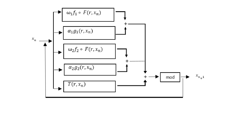
Figure 1: The combination chaotic system.

The Lyapunov exponent plot for Case (i) is given in Fig 2. From this figure we can see that for some values of $r$ the Lyapunov exponent are negative. The Bifurcation diagram for the Case (i) has been shown in Fig. 5. From this figure we can see that white lines appear in places where the Lyapunov exponent are negative. Also for Case (ii) and Case (iii) from Fig.s 2-2 we can say that for all values of $r\in(0,4]$ the Lyapunov exponent are positive. Also the Cobweb plots 4, 4 and 4 show chaotic behavior for the Case (i), Case (ii) and the Case (iii). The Fig.s 3-3 show that the Case (ii) and Case (iii) have uniform distribution over output range. Also from Fig. 4 we can see that the Case (i) has not uniform distribution over its output range. Two orbits of the Case (i) and Case(ii) are shown in Figs. 5-5. By using this figure we can see that the Case (i) and Case(ii) are much more sensitive to the starting points. By using the Lyapunov Exponents figures we can say that the Lyapunov Exponents of two examples are all larger than the Logistic map. Also the distribution of new combination chaotic system is more uniform than the distribution Logistic Tent system. Then by using suitable functions and parameters, appropriate chaotic system can be found.
In the next section, as application of the proposed chaotic system, we introduce an image encryption algorithm.

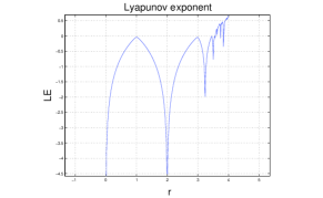
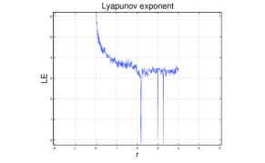
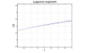
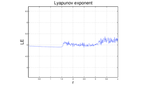
Figure 2: Lyapunov exponent plot for the (a) Logistic map, (b) Case (i), (c) Case (ii), (d) Case (iii).

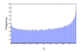
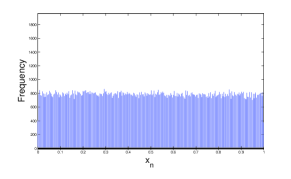
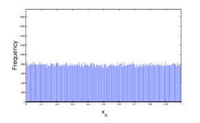
Figure 3: Histogram of the (a) Logistic Tent map, (b) Case (i), (c) Case (ii), (d) Case(iii).

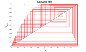
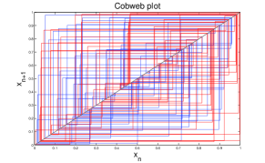
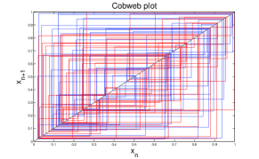
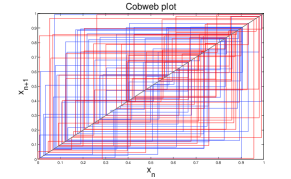
Figure 4: Cobweb plot for the (a) Logistic map, (b) Case (i), (c) Case (ii), (d) Case(iii) (blue: r=2, red: r=4).

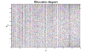
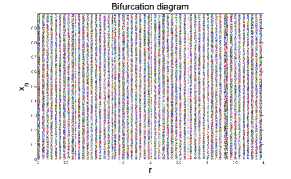
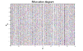
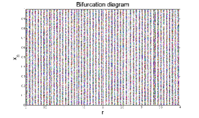
Figure 5: Bifurcation diagram for the (a) Logistic Tent map, (b) Case (i), (c) Case (ii), (d) Case(iii).

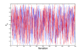
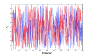
Figure 6: (a) Case (i) with $x_{0}=0.5$ (blue) and $x_{0}=0.5+10^{-15}$ (red); (b) Case (ii) with $x_{0}=0.5$ (blue) and $x_{0}=0.5+10^{-15}$ (red).

3 Proposed encryption and decryption process

In this section, we introduce some details about the proposed encryption and decryption algorithm.

3.1 Encryption process

We assume that the size of the input color image is $m\times n$. The encryption process is written in the following steps.

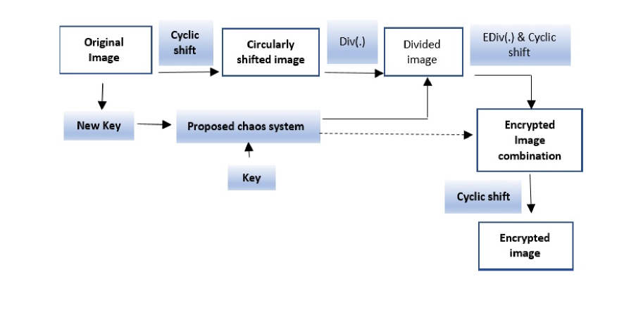
Figure 7: The encryption process of the proposed algorithm.

Step 1. For the color plain image A, we determine $y_{k},y^{0}_{k}~{}(k=1,2,3)$ as follows

$$y_{k}:=\sum_{i,j}A(i,j,k),~{}k=1,2,3,$$

$$y^{0}_{k}:=\frac{y_{k}}{m\times n\times 255},~{}k=1,2,3.$$

Therefore in this step we can find the different secret keys for different plain images. Also to generate different keys in each iteration, we consider $y^{0}_{0}$ and $y^{0}_{4}$ as random numbers in $[0,1]$. For gray scale image or binary image, we consider $y_{1}:=\sum_{i,j}A(i,j)$, $y^{0}_{1}:=\frac{y_{1}}{m\times n\times 255}$ ,$y^{0}_{0}:=rand()$ and $y^{0}_{2}:=rand()$. Also for gray scale image or binary image $y_{k},y^{0}_{k}~{}(k=3,4)$ are not used in the encryption algorithm.

Step 2. By using cyclic shift operation we find

$$A=circshift(A,[\lfloor\frac{y_{1}}{4}\rfloor~{}~{}-\lfloor\frac{y_{2}}{4}\rfloor~{}~{}\lfloor\frac{y_{3}}{4}\rfloor]),$$

$$A=circshift(A,[\lfloor\frac{y_{1}+y_{2}}{10}\rfloor~{}~{}\lfloor\frac{y_{2}+y_{3}}{10}\rfloor~{}~{}-\lfloor\frac{y_{3}+y_{1}}{10}\rfloor]),$$

where $circshift(A,r)$ circularly shifts the values in array $A$ by $r$ positions. For gray scale image or binary image, this step has been changed as follows

$$A=circshift(A,[\lfloor\frac{y_{1}}{4}\rfloor~{}~{}-\lfloor\frac{y_{1}}{3}\rfloor]),$$

$$A=circshift(A,[\lfloor\frac{2y_{1}}{10}\rfloor~{}~{}\lfloor\frac{2y_{1}}{5}\rfloor]).$$

Step 3. In this step, by using $Div(A)$ image $A$ is divided into twelve parts. In the $Div(A)$ function, image is divided into three color (red, green, blue) then each part is divided into four equal parts. However in the encryption algorithm, other division functions can be used. We can find

$$\{A^{r}_{i},A^{g}_{i},A^{b}_{i}\}_{i=1}^{4}=Div(A).$$

Step 4. We define $\Lambda(y^{0},r,n)$ as follows

$$\Lambda(y^{0},r,n):=(x_{0},x_{1},\ldots,x_{n-1}),$$ (3.1)

where $x_{i}$ $(i=1,\ldots,n-1)$ are defined by using (2) with $x_{0}=y^{0}$ and parameter $r$. Also we consider $\Omega(K_{i},r)$ for all $i\in\{1,2,3,4\}$ as a matrix with the following elements

$$\Omega(K_{i},r)(1,:):=\Lambda(y^{0}_{i},r_{i},\lfloor n/2\rfloor),~{}i=1,3,$$ (3.2)

$$\Omega(K_{i},r)(1,:):=\Lambda(y^{0}_{i},r_{i},n-\lfloor n/2\rfloor),~{}i=2,4,$$ (3.3)

$$\Omega(K_{1},r)(2:\lfloor m/2\rfloor,j):=\Lambda(\Omega(K_{1},r_{1})(1,j),r_{1},\lfloor n/2\rfloor)^{T},~{}j=1,\ldots\lfloor n/2\rfloor,$$ (3.4)

$$\Omega(K_{2},r)(2:\lfloor m/2\rfloor,j):=\Lambda(\Omega(K_{2},r_{2})(1,j),r_{2},n-\lfloor n/2\rfloor)^{T},~{}j=1,\ldots,n-\lfloor n/2\rfloor,$$ (3.5)

$$\Omega(K_{3},r)(2:m-\lfloor m/2\rfloor,j):=\Lambda(\Omega(K_{3},r_{3})(1,j),r_{3},\lfloor n/2\rfloor)^{T},~{}j=1,\ldots\lfloor n/2\rfloor,$$ (3.6)

$$\Omega(K_{4},r)(2:m-\lfloor m/2\rfloor,j):=\Lambda(\Omega(K_{4},r_{4})(1,j),r_{4},n-\lfloor n/2\rfloor)^{T},~{}j=1,\ldots,n-\lfloor n/2\rfloor.$$ (3.7)

(a)  For $i=1,\ldots,4$ we find

$$K_{i}:=\Lambda(y^{0}_{i},r_{i},\lfloor\frac{n}{2}\rfloor),$$

$$t_{i}:=mod(K_{i}(1,\lfloor\frac{n}{2}\rfloor)\times 10^{5},m\times n).$$

Also for $i=0$ we define

$$t_{0}:=\lfloor\frac{\sum^{4}_{i=1}t_{i}}{4}\rfloor,$$

$$K_{0}:=\Lambda(y^{0}_{0},r_{0},m\times n).$$

(b)  We define $Z^{1}_{i},Z^{2}_{i}~{}(i=0,\ldots,4$) as

$$Z^{1}_{i}:=\Omega(K_{i},r^{i})\times 255,$$

$$Z^{2}_{i}:=circshift(Z^{1}_{i},t_{i}).$$

Also $Z^{j}_{0}~{}(j=1,2)$ are defined as follows

$for~{}i=1:m~{}do$

$~{}~{}~{}~{}for~{}j=1:n~{}do$

$~{}~{}~{}~{}~{}~{}Z^{1}_{0}(i,j):=K_{0}(1,j+(i-1)n)\times 255,$

$~{}~{}~{}~{}end$

$end$

$$Z^{2}_{0}:=circshift(Z^{1}_{0},-t_{0}),$$

(c) By using bitxor operation matrixs $A^{j}_{i}(i=1,2,3,4,~{}j=r,g,b)$ are encrypted as follows

$for~{}i=1:4do$

$~{}~{}~{}~{}for~{}j=r,g,b~{}do$

$~{}~{}~{}~{}~{}~{}~{}~{}for~{}w=1:2do$

$~{}~{}~{}~{}~{}~{}~{}~{}~{}~{}DA^{j}_{i}:=bitxor(A^{j}_{i},Z^{w}_{i}),$

$~{}~{}~{}~{}~{}~{}~{}~{}end$

$~{}~{}~{}~{}end$

$end$

Step 6. In the encryption algorithm, the inverse function of the $Div(\cdot)$ is shown by $EDiv(\cdot)$.

(a) By using the inverse function of the $Div(\cdot)$ we find

$$EA:=EDiv(\{DA^{r}_{i},DA^{g}_{i},DA^{b}_{i}\}_{i=1}^{4}),$$

where $EA$ denotes the joined encrypted image.

(b) We transform matrix $EA$ as follows

$$EA(:,:,1)=circshift(EA(:,:,1),[-y_{1}+t_{0}~{}~{}t_{0}]),$$

$$EA(:,:,2)=circshift(EA(:,:,2),[t_{0}~{}~{}-y_{2}+t_{0}]),$$

$$EA(:,:,3)=circshift(EA(:,:,3),[t_{0}~{}~{}-y_{3}+t_{0}]).$$

(c) The final encrypted image is found as follows

$for~{}i=1:3$

$~{}~{}~{}~{}~{}~{}EA(:,:,i)=bitxor(EA(:,:,i),Z^{1}_{0}),$

$~{}~{}~{}~{}~{}~{}EA(:,:,i)=bitxor(EA(:,:,i),Z^{2}_{0}),$

$end$

$$EA=circshift(EA,[y_{1}+y_{2}~{}~{}y_{2}+y_{3}~{}~{}y_{1}+y_{3}]),$$ (3.8)

$$EA=circshift(EA,[\lfloor\frac{y_{1}}{50}\rfloor~{}~{}\lfloor\frac{y_{2}}{50}\rfloor~{}~{}-\lfloor\frac{y_{3}}{50}\rfloor]).$$ (3.9)

For gray scale image or binary image, Eq.s (3.8)-(3.9) has been changed as follows

$$EA=circshift(EA,[y_{1}~{}~{}-2y_{1}),$$

$$EA=circshift(EA,[\lfloor\frac{y_{1}}{50}\rfloor~{}~{}-\lfloor\frac{y_{1}}{35}\rfloor]).$$

3.2 Decryption process

The decryption process is the inverse process of the encryption process, so we remove the decryption details.

4 Simulation results and security analysis

4.1 Simulation results

In order to illustrate the encryption algorithm results and security analysis, we consider some test problems. In this section in all figures we use Case (ii) in the encryption process. We have computed the numerical results by MATLAB 7.11.0 programming. As plain images, we use color images “Sailboat on lake” , “Airplane (F-16)” ($512\times 512\times 3$ pixels), “Lena” ($256\times 256\times 3$, $512\times 512\times 3$ pixels) and gray scale image “Lena” ($256\times 256$ , $512\times 512$ pixels), “girl” ($256\times 256$ pixels). Also “Horse” ($444\times 455$ pixels) is used as binary image. The simulations results are given in Figs. 8-14. In Figs. 8-9 we show the encryption algorithm results. The binary image has only two pixel values 0 and 1, therefore it is a difficult case for encryption. As can be seen in the Fig.9, by using the proposed algorithm for the binary image, the image is changed to a noise-like encrypted image with flat histogram. The running time of encryption and decryption are shown in Table 1.

Table 1: Encryption and decryption times of the color images by using Case (ii).

Image	Encryption time	Decryption time
Lena (512 $\times$ 512)	1.130 s	1.044 s
Sailboat on lake	1.105 s	1.044 s
Airplane (F-16)	1.139 s	1.024 s

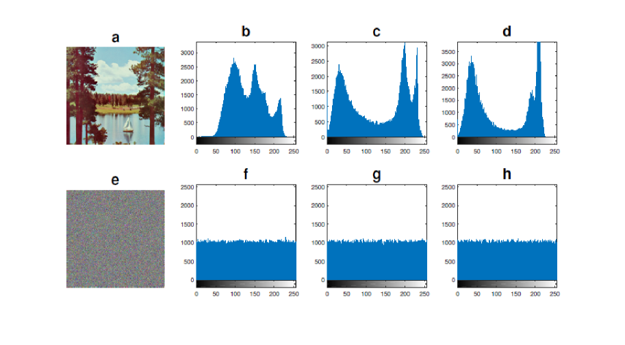
Figure 8: (a) Original image, (b-c-d) Histograms of the R, G, B components of the original image, (e) Encrypted image, (f-g-h) Histograms of the R, G, B components of the encrypted image (Sailboat on lake).

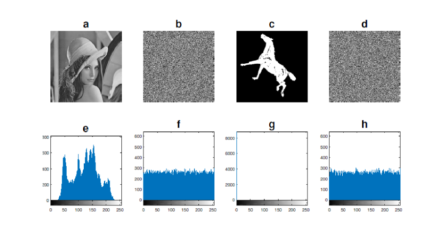
Figure 9: (a-b) Original and encrypted image, (e-f) Histograms of the original image and encrypted image (Lena -$256\times 256$), respectively, (c-d) Original and encrypted image, (g-h) Histograms of the original image and encrypted image (Horse), respectively.

4.2 Security analysis

In this subsection, the different security parameters are discussed, for details see [11, 12].

4.2.1 Security key analysis

From the proposed algorithm, we can say that the security keys of the algorithm are composed of ten parameters $\{r_{i}\}^{4}_{n=0}$ and $\{y^{0}_{i}\}^{4}_{n=0}$, The range for $r_{i}~{}(i=0,\ldots 4)$ are $(0,4]$ Also $y^{0}_{i}~{}(i=0,\ldots 4)$ are in range of $[0,1]$. If in the image encryption algorithm we consider the precision as $10^{-15}$ the key space is almost $10^{150}$, and this space is sufficiently large to resist the brute force attack.
To show key sensitivity, in the encryption process we consider key as follows (this key is used to obtain all results)

$$k:=(r_{0},r_{1},r_{2},r_{3},r_{4})=(2,1,2,3.5,1.75).$$ (4.1)

In the decryption process, we use a small change for $r_{0}$ as $r_{0}=2+10^{-15}$, we consider new key as $K_{1}$. Simulation results in Fig. 10 show that by using new key we can not reconstruct the original image. Therefore, the proposed algorithm has high key sensitivity.

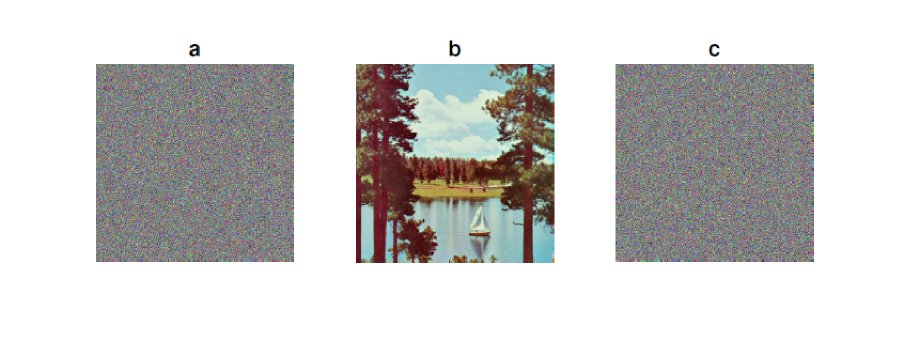
Figure 10: (a) Encrypted image (Sailboat on lake), (b) Decrypted image by using $K$, (c) Decrypted image by using $K_{1}$.

4.2.2 Statistical analysis

In this section, we study statistical analysis as part of the security analysis. It is clear that a good encrypted image should be unrecognized hence the correlation values of a good encrypted image are close to zero. Table 3 shows the correlation values for the original images and encrypted images. We have found the correlation values using formula [13]

$$C_{xy}=\frac{E[(x-\mu_{x})(y-\mu_{y})]}{\sigma_{x}\sigma_{y}},$$ (4.2)

where $E[\cdot]$ denotes the expectation value, $\mu$ is the mean value and $\sigma$ represents standard deviation. From Table 3, we can see that the original images have high correlation values while encrypted images have very low correlation values. Also correlation distributions for the original image and encrypted image of Lena image are shown in Fig.11.

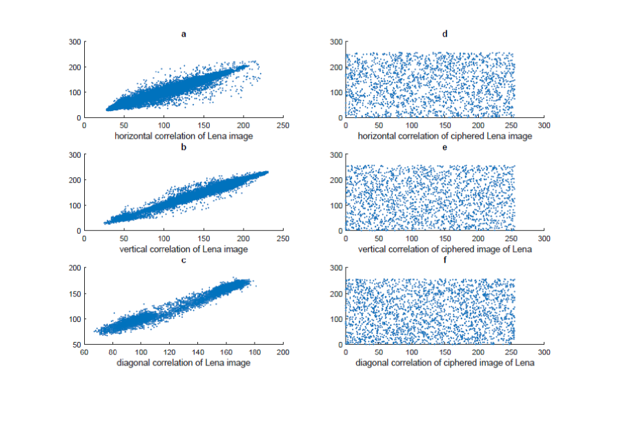
Figure 11: Correlation of neighborhood pixels at different directions before and after encryption of Lena ( 512 $\times$ 512 pixels).

Table 2: Correlation coefficients of the encrypted color image of ”Sailboat on lake”.

Chaos map	Component	Horizontal	Vertical	Diagonal	Diagonal
				(lower left to top right)	(lower right to top left)
	R	-0.0027	-0.0003	-0.0016	0.0019
Case (i)	G	0.0009	-0.0019	-0.0008	0.0027
	B	-0.0017	-0.0005	-0.0019	0.0024
	R	0.0007	-0.0003	-0.0006	-0.0002
Case (ii)	G	0.0029	-0.0005	-0.0003	-0.0003
	B	-0.0007	0.0009	0.0010	-0.0023
	R	0.0003	0.0018	0.0020	0.0027
Case (iii)	G	0.0029	-0.0005	-0.0028	0.0030
	B	-0.0007	-0.0021	0.0007	-0.0021
	R	-0.0029	0.0011	0.0028	-0.0005
Logistic Tent	G	-0.0009	0.0033	0.0035	-0.0002
	B	-0.0009	0.0025	0.0012	0.0005
	R	0.9558	0.9541	0.9373	0.9420
Original image	G	0.9715	0.9663	0.9510	0.9530
	B	0.9710	0.9694	0.9512	0.9530

Table 3: Comparison of Correlation coefficients of image of “Lena” ($512\times 512$).

Method	Horizontal	Vertical	Diagonal
The proposed	-0.0036	-0.0020	-0.0026
Method in [14]	0.0139	0.0073	0.0104

The other test is the information entropy. The values of entropy are in range of $[0,8]$. This test is used for evaluating the randomness of an image. If the value of entropy of encrypted image is close to the maximum value means the excellent random property. The information entropy is defined as follows [12]

$$H(k)=-\sum^{w-1}_{i=0}P(k_{i})\log_{2}P(k_{i}),$$ (4.3)

where $w$ is the gray level and $P(\cdot)$ denotes the probability of symbol. Results for the information entropy are tabulated in Table 4. From Table 4, we can say that test results for the encryption algorithm are close to the maximum value. Also Figs. 8-9 show that the histograms of plain images are not flat while the histograms of encrypted images are in flat distributions.

From the above discussion, it can be concluded that the proposed algorithm has stronger ability to resist statistical attacks.

Table 4: Informaion entropies of the encrypted color image.

Chaos map	Image		R		G		B
	Lena ($512\times 512\times 3$)		7.9970		7.9972		7.9970
Case (i)	Sailboat on lake		7.9993		7.9993		7.9992
	Airplane (F-16)		7.9994		7.9992		7.9993
	Lena ($512\times 512\times 3$)		7.9967		7.9967		7.9972
Case (ii)	Sailboat on lake		7.9992		7.9993		7.9993
	Airplane (F-16)		7.9994		7.9993		7.9994
	Lena ($512\times 512\times 3$)		7.9970		7.9973		7.9975
Case (iii)	Sailboat on lake		7.9994		7.9993		7.9993
	Airplane (F-16)		7.9991		7.9992		7.9994
	Lena ($512\times 512\times 3$)		7.9975		7.9970		7.9970
Logistic Tent	Sailboat on lake		7.9993		7.9992		7.9993
	Airplane (F-16)		7.9993		7.9994		7.9994

4.2.3 Sensitivity analysis

NPCR (Number of Pixels change Rate) denotes the number of pixels change rate while one pixel of plain image changed. Also UACI (Unified Average Changing Intensity) measures the average intensity of differences between the plain image and encrypted image. The ideal value for NPCR is $100\%$ while the ideal value for UACI is $33.\overline{33}\%$. When the value of NPCR gets closer to $100\%$, the encryption algorithm is more sensitive to the changing of plain image, therefore the algorithm can effectively resist plaintext attack. Also when the value of NPCR gets closer to $33.\overline{33}\%$, the proposed algorithm can effectively resist differential attack. In computing, we consider NPCR and UACI as follows

$$NPCR=\frac{\sum_{i,j}D(i,j)}{m\times n}\times 100\%,$$ (4.4)

$$UACI=\frac{1}{m\times n}\big{[}\frac{\sum_{i,J}|C_{1}(i,j)-C_{2}(i,j)|}{255}\big{]}\times 100\%,$$ (4.5)

where

$$D(i,j):=\left\{\begin{array}[]{ll}1,&when~{}C_{1}(i,j)\neq C_{2}(i,j),\\ \\ 0,&when~{}C_{1}(i,j)=C_{2}(i,j).\\ \end{array}\right.$$ (4.9)

In above formulae, $C_{1}(i,j)$ and $C_{2}(i,j)$ are denoted the cipher image before and after one pixel of the plain image is changed. In the Lena, Sailboat on lake and Airplane images, $A(200,150,1)$, $A(100,250,2)$ and $A(180,334,3)$ are changed to 0, respectively. As can be seen in Table 5 , results are close to ideal values.

Table 5: UACI and NPCR of the encrypted color image.

Image	UACI			NPCR
	R	G	B	R	G	B
Lena ($512\times 512\times 3$)	33.4457	33.5589	33.5243	99.6078	99.6140	99.6033
Sailboat on lake	33.4617	33.3928	33.5061	99.6082	99.6231	99.6048
Airplane (F-16)	33.4744	33.4482	33.4813	99.6353	99.6059	99.6021

4.2.4 Noise and Data loss attacks

In continuation of discussion, by using the simulation results we study noise and data loss attacks. In real applications, a part of the encrypted image may be lost during transmission. A proper encryption algorithm should resist the data loss and noise attacks. In Fig. 12, we remove $200\times 200$ of encrypted image. In fact we consider $A(80:280,80:280)=0_{200\times 200}$. Also in Fig. 13, for encrypted image we add Gaussian noise with zero-mean and different variance. After the decryption process, we can see that the reconstructed images contain most of original visual in formation and we can recognize the original image from decrypted image.

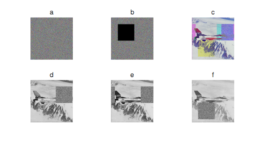
Figure 12: Cropped attack experiment: (a) Encrypted image, (b) cropped attack image, (c) Decryption result, (d-e-f) Decryption result for the R, G, B components, respectively.

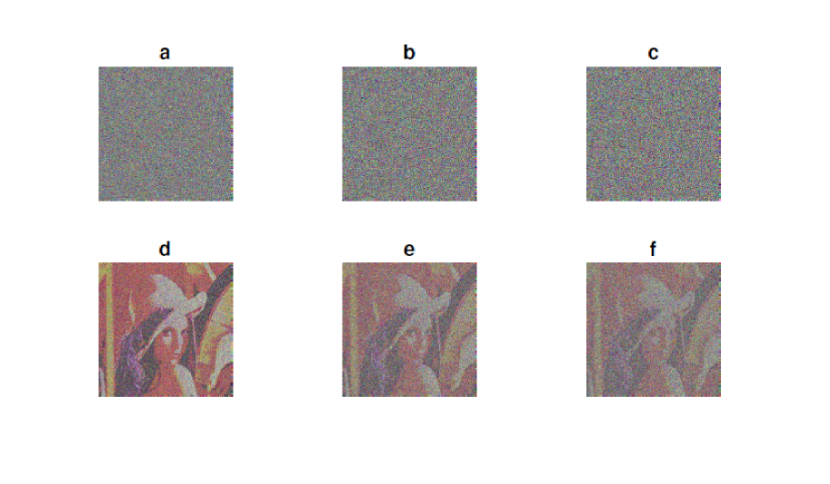
Figure 13: Noise attack experiment with Gaussian noise (a-b-c) noise attack image with var=0.1,0.4,0.8, respectively, (d-e-f) decryption with var=0.1,0.4,0.8, respectively.

4.2.5 Chosen-plain text attack

In the encryption algorithm, in Step 1, random numbers are used. So this algorithm create different encrypted image each time when the encryption algorithm is applied to the same image. In Fig. 14 we use $K$ as key and we run the encryption algorithm twice. The first and second encrypted image are consider as $C_{1}$ (Fig. 14(b)) and $C_{2}$ (Fig. 14(c)) , respectively. To illustrate the difference between the two images, we use pixel-to-pixel difference as $|C_{1}-C_{2}|$. As can be seen in Fig. 10, two encrypted images are different. Then the our algorithm is able to withstand the chosen-plain text attack.

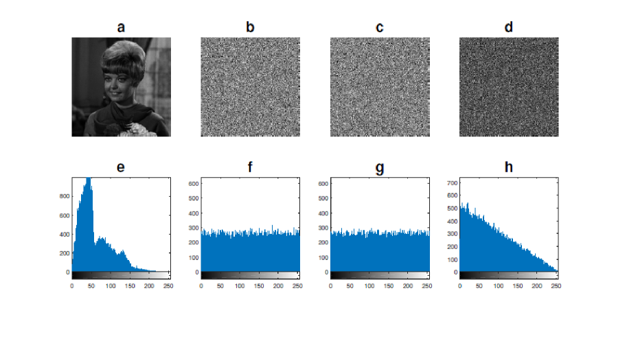
Figure 14: (a-e) The original image and its histogram, (b-f) the first encrypted image and its histogram, (c-g) the second encrypted image and its histogram, (d-h) the pixel-to-pixel difference and its histogram.

5 Conclusion

In this paper, we have constructed a new combination chaotic system based on Logistic and Tent systems. By using this new combination chaotic system a large number of chaotic map can be produced. Also we have proposed a new image encryption algorithm based on combination chaotic system. It is shown that the proposed encryption algorithm can effectively resist differential, statistical, noise, data loss, chosen-plain text attacks.

References

- [1] R. Matthews, On the derivation of a chaotic encryption algorithm, Cryptologia 4 (1989) 29-42.
- [2] Ü. Çavuşoğlu, S. Kaçarb, I. Pehlivanb, A. Zengina, Secure image encryption algorithm design using a novel chaos based S-Box, Chaos, Solitons Fractals 95 (2017) 92-101.
- [3] A. Kanso, M. Ghebleh, An algorithm for encryption of secret images into meaningful images, Optics and Lasers in Engineering 90 (2017) 196-208.
- [4] X.Y. Wang, L. Yang, R.Liu, A. Kadir, A chaotic image encryption algorithm based on perceptron model, Nonlinear Dynamics 62 (2010) 615-621
- [5] G. Gu, J. Ling, A fast image encryption method by using chaotic 3D cat maps, Optik - International Journal for Light and Electron Optics 125 (2014) 4700-4705.
- [6] M. Kumar, A. Vaish, Encryption of color images using MSVD in DCST domain, Optics and Lasers in Engineering 3 (1990) 278-285.
- [7] M. Ausloos, M. Dirickx, The Logistic Map and the Route to Chaos: From the Beginnings to Modern Applications, Springer 2006.
- [8] R. Hilborn, Chaos and Nonlinear Dynamics: An Introduction for Scientists and Engineers, Oxford University Press 2000.
- [9] S.C. Satapathy, A. Govardhan, K.S. Raju, J.K. Mandal, Emerging ICT for Bridging the Future - Proceedings of the 49th Annual Convention of the Computer Society of India (CSI), Springer International Publishing Switzerland 2015.
- [10] S. Lynch, Dynamical Systems with Applications using MATLAB , Second Edition, Birkhäuser Boston 2014.
- [11] A. Uhl, A. Pommer, Image and Video Encryption From Digital Rights Management to Secured Personal Communication, Springer 2004.
- [12] F.A El-Samie, H.H. Ahmed, I.F. Elashry, M.H. Shahieen, O.S. Faragallah, E.M. El-Rabaie, S.A. Alshebeili, Image Encryption: A Communication Perspective, CRC Press 2014.
- [13] N. Zheng, J. Xue, Statistical learning and pattern analysis for image and video processing, Springer Science Business Media, 2009.
- [14] G. Gu, J. Ling, A fast image encryption method by using chaotic 3D cat maps, Optik-International Journal for Light and Electron Optics, 17 (2014) 4700-4705.