Detecting Noteheads in Handwritten Scores
with ConvNets and Bounding Box Regression

Abstract

Noteheads are the interface between the written score and music. Each notehead on the page signifies one note to be played, and detecting noteheads is thus an unavoidable step for Optical Music Recognition. Noteheads are clearly distinct objects; however, the variety of music notation handwriting makes noteheads harder to identify, and while handwritten music notation symbol classification is a well-studied task, symbol detection has usually been limited to heuristics and rule-based systems instead of machine learning methods better suited to deal with the uncertainties in handwriting. We present ongoing work on a simple notehead detector using convolutional neural networks for pixel classification and bounding box regression that achieves a detection f-score of 0.97 on binary score images in the MUSCIMA++ dataset, does not require staff removal, and is applicable to a variety of handwriting styles and levels of musical complexity.

I Introduction

Optical Music Recognition (OMR) attempts to extract musical information from its written representation, the musical score. Musical information in Western music means an arrangement of notes in musical time. There are many ways in which music notation may encode an arrangement of notes, but an elementary rule is that one note is encoded by one notehead.

Given the key role noteheads play, detecting them – whether implicitly or explicitly – is unavoidable for OMR. At the same time, if one is concerned only with replayability and not with re-printing the input, noteheads are one of the few music notation symbols that truly need detecting (i.e., recovering their existence and location) in the score: most of the remaining musical information can then be framed in terms of classifying the noteheads with respect to their properties such as pitch or duration; bringing one to the simpler territory of music notation symbol classification.

Music notation defines noteheads so that they are quickly discernible, and from printed music, detecting noteheads has been done using segmentation heuristics such as projections [1, 2] or morphological operators [3, 4]. However, in handwritten music, noteheads can take on a variety of shapes and sizes, as illustrated by fig. 1, and handwriting often breaks the rules of music notation topology: noteheads may overlap (or separate from) symbols against the rules. Robust notehead detection in handwritten music thus invites machine learning.

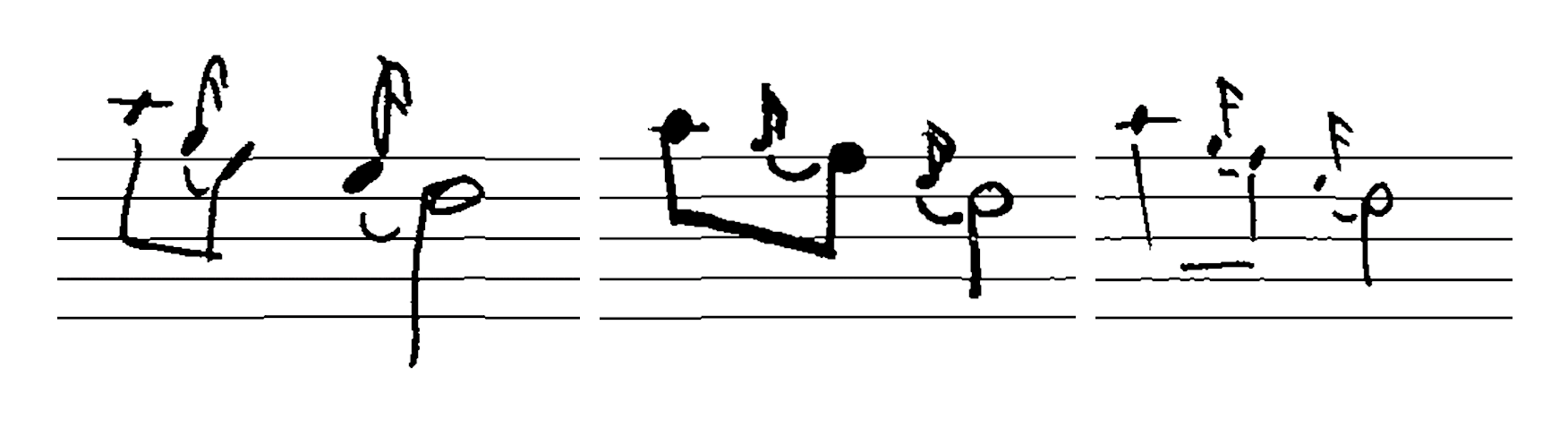
Figure 1: The variety of noteheads and handwriting styles: full, empty, and grace noteheads.

Our contribution is a simple handwritten notehead detector, which achieves a detection performance of 0.97 on binary images across scores of various levels of musical complexity and handwriting styles. At the heart of the detector is a small convolutional neural network based on the RCNN family of models, specifically Faster R-CNN [Ren2015bs]. Within the traditional OMR pipeline as described by Rebelo et al. [5], our work falls within the symbol recognition stage, specifically as a crucial subset of the “isolating primitive elements” and jointly “symbol classification” steps; however, it does not require staff removal. In the following sections, we describe the detector in detail, demonstrate its performance in an experimental setting, describe its relationship to previous work, and discuss its limitations and how they can be overcome.

II Notehead Detector

The notehead detection model consists of three components: a target pixel generator that determines which regions the detector should attend to, a detection network that jointly decides whether the target pixel belongs to a notehead and predicts the corresponding bounding box, and an additional proposal filter that operates on the combined predictions of the detection network and decides whether the proposed bounding boxes really correspond to a notehead.

II-A Target Pixel Generator

The target pixel generator takes a binary score image and outputs a set of $X,t$ pairs, where $X$ is the input for the detection network corresponding to the location $t=(m,n)$ of a target pixel. From training and validation data, it also outputs $y=(c,b)$ for training the detection network. The class $c$ is $1$ if $t$ lies in a notehead and $0$ otherwise; $b$ encodes the bounding box of the corresponding notehead relative to $t$ if $c=1$ (all values in $b$ are non-negative; they are intepreted as distance form $t$ to the top edge of the bounding box of the notehead, to its left edge, etc.); if $c=0$, $b$ is set to $(0,0,0,0)$. The network outputs are described by Fig. 2.

The detection network input $X$ is a patch of the image centered on $t$. The patch must have sufficient size to capture enough context around a given target pixel, to give the network a chance to implicitly operate with rules of music notation, e.g. to react to the presence of a stem or a beam in certain positions. We set the patch size to 101x101 (derived from $1.2*staff\_height$), and downscale to 51x51 for speed.

At runtime, we use all pixels of the morphological skeleton as target pixels $t$. If one correctly classifies the skeleton pixels and then dilates these classes back over the score, we found over 97 % of individual foreground pixels classified correctly (measured on the MUSCIMA++ dataset [6]), making the skeleton a near-lossless compression of the score to about 10 % of the original foreground pixels.

For training, we randomly choose $k$ target pixels for each musical symbol in the training set, from the subset of the skeleton pixels that lies within the given symbol. In non-notehead symbols, we forbid extracting skeleton pixels that are shared with overlapping noteheads: we simply want to know whether a given pixel $t$ belongs to a notehead or not. (This is most pronounced in ledger lines crossing noteheads.) Setting $k>1$ did not improve detection performance; we suspect this is because all $X$s from a symbol $S$ are highly correlated and therefore do not give the network much new information.

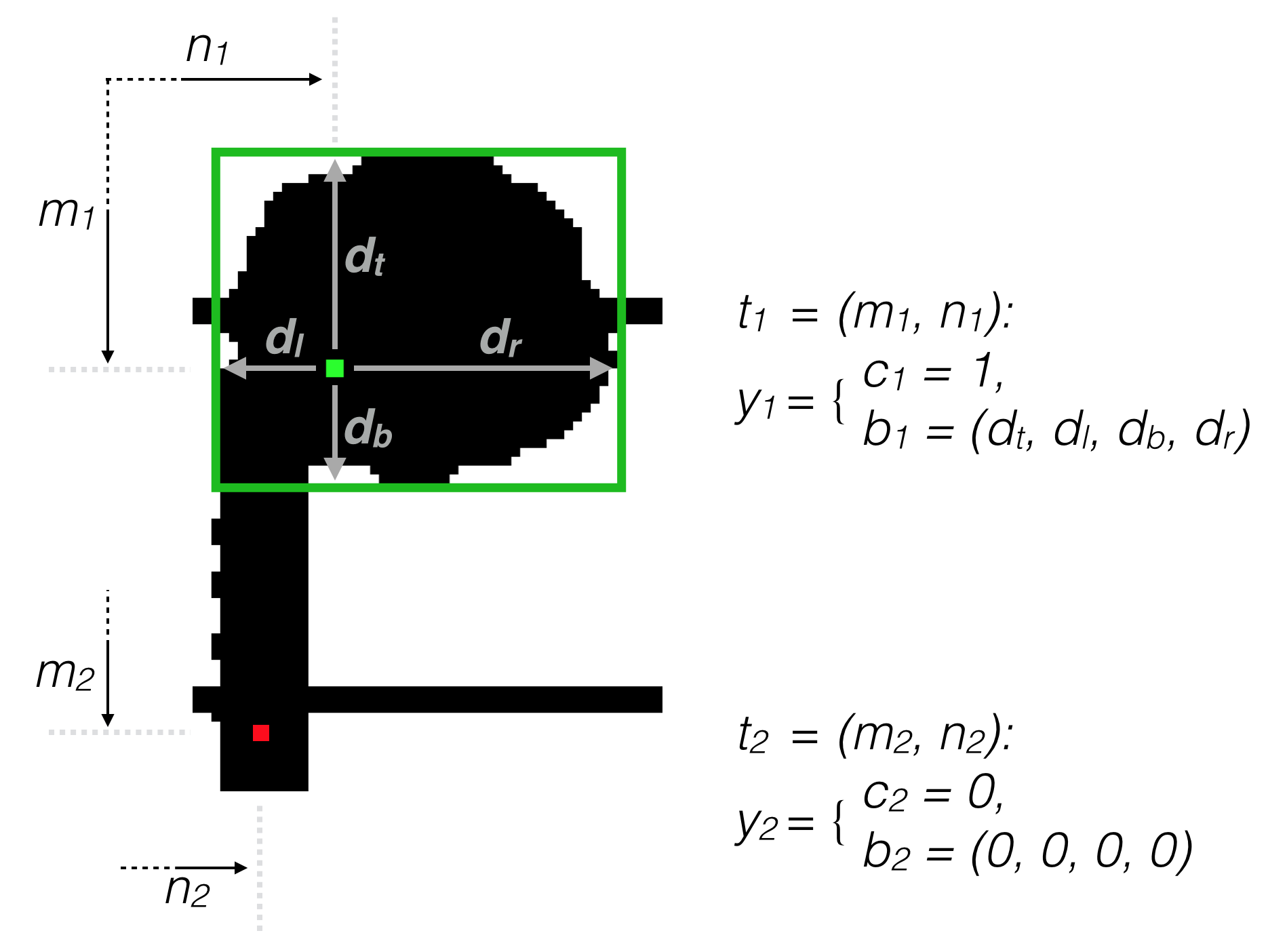
Figure 2: The outputs which the detection network is learning for each target pixel, the green $t_{1}$ and red $t_{2}$: its class $c$, and the position $b$ of the target pixel inside the notehead’s bounding box – set to all zeros when $t$ does not belong to a notehead, as seen in $y_{2}$.

II-B Detection Network

The detection network handles most of the “heavy lifting”. It is a small convolutional network with two outputs: a binary classifier (notehead-or-not) and a bounding box regressor. The inputs to the network are the patches $X_{1}\dots X_{N}$ extracted by the target pixel generator; the ground truth for training are the class and bounding box information $y_{1}=(c_{1},b_{1}),\dots,y_{N}$ described in II-A. This follows the architecture of Faster R-CNN [7], but as our inputs are not the natural images on which VGG16 [8] was trained, we train our own convolutional stack. (See Sec. IV for a more thorough comparison.)

Our network has four convolutional layers, with the first two followed by max-pooling with pool size 2x2. Dropout is set to 0.25 after the max-pooling layers and 0.125 after the remaining convolutional layers. The output of the fourth convolutional layer is then densely connected to the classification output and the bounding box regression outputs. The convolutional layers use $tanh$ activation rather than ReLU: we found that this made learning converge faster, although we are still unsure why. Details are given in table I.

The classification output uses cross-entropy loss; the bounding box regression output uses mean squared error loss, weighted at 0.02 of the classification loss. The network was implemented using the Keras library [9].

II-C Notehead Proposal Filter

The detection network outputs correspond to individual target pixels, selected by the generator; we now combine these results into noteheads.

We take the union of all bounding boxes output by the detection network for target pixels with predicted class $c=1$, and we use bounding boxes of the connected components of this union as notehead proposals. We then train a classifier of notehead proposals. This classifier can take into account all the network’s decisions, as well as other global information; however, it can only fix false positives, – if the network misses a notehead completely, the filter cannot find it. However, the detection network in the described setting achieves good recall and has more trouble with precision, so such filtering is appropriate.

The features we extract for proposal filtering from each proposal region $B_{1},\dots,B_{j}$ are:

• $h(B)$, the height of $B$,

• the ratio $\hat{h}(B)$ of $h(B)$ to the average height of $B_{1},\dots,B_{j}$,

• $w(B)$, the width of $B$, and analogously $\hat{w}(B)$,

• area $a(B)=h(B)*w(B)$, analogously $\hat{a}(B)$,

• the no. of foreground pixels in $B$: $N_{fg}(B)$, and the proportion $p_{fg}(B)=N_{fg}(B)/a(B)$,

• $N^{+}(B)$, the no. of positively classified target pixels $t^{+}\in B$,

• $p^{+}(B)$, the proportion of such target pixels to all in $t^{+}\in B$,

• the ratio $\hat{N}^{+}(B)$,

• equiv. for non-notehead pixels $t^{-}\in B$: $N^{-}(B)$, $p^{-}(B)$, $\hat{N}^{-}(B)$,

• ”soft” sum of noteheadedness: $S^{+}(B)=\sum_{t^{+}\in B}P(+\mid t)$,

• again, the ratio to the average $S^{+}(B)$ in the image: $\hat{S}^{+}(B)$.

• $l(B)$: how much to the left in the input image $B$ is.

The ratio features ($\hat{w}(B)$, etc.) are designed to simulate invariance to individual handwriting styles. Also, beyond features based on detection network outputs, the left-ness $l(B)$ is used to find false positives in clefs.

For training the proposal filter, we consider correct each notehead proposal that has Intersection-over-Union (IoU) with a true notehead above 0.5. We use a Random Forest with 300 estimators, a maximum depth of 8, and a minimum of 3 samples in each leaf.

III Experiments

We now describe the experimental setup in which the detector was tested: the dataset, evaluation procedure, and experimental results.

III-A Data

For experiments, we use the MUSCIMA++ dataset of Hajič jr. and Pecina [6], based on the underlying images of CVC-MUSCIMA by Fornés et al. [10]. The dataset contains 140 binary images. There are 20 pages of music, each as transcribed by 7 of the 50 writers of CVC-MUSCIMA; all the 50 CVC-MUSCIMA writers are represented in MUSCIMA++. The scores all use the same staffline and staffspace heights (see [10] for details). We use a test set that contains one of each of the 20 pages, chosen so that no page by the writers of the test set pages is seen in the training set (we first want to see how the system generalizes to unseen handwriting style, rather than unseen notational situations). When extracting ground truth, we did not differentiate between different noteheads (full, empty, grace-note).

We used the first 100 of the remaining 120 images as the training set for the detection network, and the other 20 as the validation set. As we are training on only one sample target pixel per musical symbol, this amounted to 65015 training instances. Using the Adam optimizer, training converged after 8-9 epochs.

The outputs of the network on the dev set were then included for training the notehead proposal filter, together with the first 50 images from the training set. (The dev set better approximates the inputs to the proposal filter at runtime conditions, when the detection network runs on images never seen in training.)

Layer	Dropout	Activation	Size
conv1	–	tanh	32 filters 5x5
pool1	0.25	–	pool 2x2
conv2	–	tanh	64 filters 3x3
pool2	0.25	–	pool 2x2
conv3	0.125	tanh	64 filters 3x3
conv4	0.125	tanh	64 filters 3x3
clf.	–	sigmoid	1
bb. reg.	–	ReLU	4

TABLE I: Detection Network Architecture. (Both the classification and bounding box regression output layers are densely connected to conv4.)

III-B Evaluation Procedure

We evaluate notehead detection recall and precision. A notehead prediction that has IoU over 0.5 with a true notehead is a hit. Furthermore, we count each predicted notehead that completely contains a true notehead. This non-standard way of counting hits was chosen because in some cases, the bounding box regression produced bounding boxes that were symmetrically ”around” the true notehead, but slightly too large, to the extent that it set IoU too low due to the predicted notehead’s contribution to the union term. However, a symmetrically larger bounding box (when oversized only to the limited extent present in the model outputs) does not impede recovering the notehead’s relationship to other musical symbols, e.g., stafflines, and this adjustment should therefore give the reader a better grasp of the detector’s actual useful performance.

III-C Results

On average, the detector achieves a recall of 0.96 and precision of 0.97. Among the test set, there were two images where recall fell to around 0.9: 0.87 for CVC-MUSCIMA image W-12_N-19 (writer 12, page 19), and 0.91 for W-29_N-10, due to the detection network’s errors on empty noteheads in the middle of chords, full noteheads in chords with a handwriting style where the notehead is essentially just a thickening or straight extension of the stem, and certain grace notes; there are also problems with whole notes on the “wrong” side of the stem in W-39_N-20. Aside from these situations, the detector rarely misses a note.

The detection network itself has an average pixel-wise recall on the positive class of 0.94 (again, the average is lowered mostly by the three problematic images, rather than evenly distributed errors), but precision only 0.78 (even though most of the false positives are skeleton pixels in the close vicinity of actual noteheads). The notehead detection recall without post-filtering is 0.97 and precision is 0.81. As the false positives are clearly a much greater problem than false negatives, preliminary results to this effect on the development set motivated work on the post-filtering step. The post-filter increases detection precision by 0.16, eliminating over 84 % of all the false positives, while only introducing 1 % more false negatives.

IV Related work

Given that there was little publicly available ground truth for notehead detection until recently [6], it is hard to compare results to previous work directly. A noteworthy approach on the same CVC-MUSCIMA handwritten data was taken by Baro et al. [4]. They achieve a notehead detection f-score of 0.64 based on handcrafted rules alone, without any machine learning. This is an indication that contemporary handwritten music will need a machine-learning approach rather than the projection-based heuristics that have been used in printed music [1, 2] and applied to handwritten early music scores with recall 0.99 and precision 0.75 [3].

Convolutional neural networks have been previously successfully applied to music scores by Calvo-Zaragoza et al., for segmentation into staffline, notation, and text regions [11] or binarization [12], with convincing results that generalize over various input modes.

Our detector is inspired by the RCNN family of models, especially Faster R-CNN [7]. RCNNs were motivated by the fact that detection can be decomposed into region proposals and classification, with models such as VGG16 [8] for natural image classification obtaining near-human performance. However, the pre-trained image classification nets are too slow for a trivial sliding window approach. RCNNs use a sparse grid of proposal regions with pre-defined sizes and shapes, and train bounding box regression to locate the object of interest within the proposal region. (Faster R-CNN trains bounding box regression directly on top of the high-quality image classification features.) When combining predictions to obtain detection outputs, RCNN models then apply non-maximum suppression on the detection probability landscape obtained from predictions for each of the pre-defined proposal regions.

Together with [7], we apply joint classification and bounding box regression, but our approach differs from RCNNs in four aspects. We do not use a fixed proposal grid but generate proposal regions dynamically from the input image. Second, we cannot reuse VGG16 [8] or other powerful pre-trained image classification models for feature extraction, since they not trained on music notation data; however, because our input space is much simpler, we can train the convolutional layer stack directly. Third, we use a separate classifier to take advantage of the network outputs for related proposal regions, combining the network’s ”votes” on multiple closely related inputs more generally than simply non-maxima suppression. A final subtle distinction is that we are not just looking for a notehead anywhere in the proposal region; we want the center pixel of the region to be part of the notehead, constraining bounding box regression outputs roughly to the average size of a notehead even with a much larger input patch.

V Discussion and Conclusions

We proposed an accurate notehead detector from simple image processing and machine learning components. However, ongoing work on the detector will need to address several limitations.

Our system requires binary images. The detection network can be trained on augmented grayscale data, and given the track record of convolutional networks, one would expect good performance; however, an alternate target pixel selection mechanism is needed.

A second problem is slow runtime: over a minute per MUSCIMA++ test set image on a consumer CPU. This can be mitigated by first downsampling the skeleton, and then informing the choice of more target pixels by the results, directing the network to focus only on ”hopeful” areas where it has detected a notehead.

While the binary nature of the task is appealing, the network is in fact forced to lump different symbols together. This is more pronounced in the negative class, where the variety of shapes is larger. Saliency maps for the last convolutional layer suggest that most of its filters relate to the presence of a stem; forcing the network to discriminate among more classes might force convolutional filters to distinguish specifically between noteheads and similar objects.

The final issue is generalizing past the high-quality scans of CVC-MUSCIMA images. In preliminary experiments on an early music page with low-quality binarization and some blurring and deformation, the detector gets f-score 0.85 without and 0.79 with post-filtering. The more fragile stages of the detector are at fault – a low-quality skeleton, and the correspondingly uncertain inputs for the post-filtering classifier. (The post-filtering classifier is fragile in the sense that its features are directly derived from the combined outputs of the detection network, and thus it is “conditioned” for a certain level of network performance.)

These limitations suggest a way forward: more efficient target pixel selection, applicable to grayscale images; data augmentation to simulate more real-world conditions; a more robust post-filtering step, ideally trainable jointly with the detection network; and extending the detection network to multiple output classes (which, when combined with using previous outputs in the vicinity of a given target pixel as an input to the network, can also incorporate music notation syntax more explicitly).

The simple detector has proven to be quite powerful, resistant to changes in handwriting style and most notation complexity, showcasing the potential of quite simple neural networks (and the value of a dataset). In spite of the limitations, we find this an encouraging result for offline handwritten OMR.

References

- [1] I. Fujinaga, “Optical Music Recognition using Projections,” Master’s thesis, 1988.
- [2] P. Bellini, I. Bruno, and P. Nesi, “Optical music sheet segmentation,” in Proceedings First International Conference on WEB Delivering of Music. WEDELMUSIC 2001. Institute of Electrical & Electronics Engineers (IEEE), 2001, pp. 183–190. [Online]. Available: papers2://publication/uuid/FEF468FA-2244-48DF-94C6-64246D675F15
- [3] A. Fornés, “Primitive Segmentation in Old Handwritten Music Scores,” pp. 279–290, 2006.
- [4] Arnau Baro, Pau Riba, and Alicia Fornés, “Towards the Recognition of Compound Music Notes in Handwritten Music Scores,” in 15th International Conference on Frontiers in Handwriting Recognition, ICFHR 2016, Shenzhen, China, October 23-26, 2016. IEEE Computer Society, 2016, pp. 465–470. [Online]. Available: http://dx.doi.org/10.1109/ICFHR.2016.0092
- [5] Ana Rebelo, Ichiro Fujinaga, Filipe Paszkiewicz, Andre R. S. Marcal, Carlos Guedes, and Jaime S. Cardoso, “Optical Music Recognition: State-of-the-Art and Open Issues,” Int J Multimed Info Retr, vol. 1, no. 3, pp. 173–190, Mar 2012. [Online]. Available: http://dx.doi.org/10.1007/s13735-012-0004-6
- [6] J. Hajič, jr. and P. Pecina, “In Search of a Dataset for Handwritten Optical Music Recognition: Introducing MUSCIMA++,” ArXiv e-prints, Mar. 2017.
- [7] Shaoqing Ren, Kaiming He, Ross B. Girshick, and Jian Sun, “Faster R-CNN: Towards Real-Time Object Detection with Region Proposal Networks,” in Advances in Neural Information Processing Systems 28: Annual Conference on Neural Information Processing Systems 2015, December 7-12, 2015, Montreal, Quebec, Canada, C. Cortes, N. D. Lawrence, D. D. Lee, M. Sugiyama, and R. Garnett, Eds., 2015, pp. 91–99. [Online]. Available: http://papers.nips.cc/paper/5638-faster-r-cnn-towards-real-time-object-detection-with-region-proposal-networks
- [8] Karen Simonyan and Andrew Zisserman, “Very Deep Convolutional Networks for Large-Scale Image Recognition,” CoRR, vol. abs/1409.1556, 2014. [Online]. Available: http://arxiv.org/abs/1409.1556
- [9] François Chollet, “Keras,” https://github.com/fchollet/keras, 2017. [Online]. Available: https://github.com/fchollet/keras
- [10] A. Fornés, A. Dutta, A. Gordo, and J. Lladós, “CVC-MUSCIMA: a ground truth of handwritten music score images for writer identification and staff removal,” International Journal on Document Analysis and Recognition (IJDAR), vol. 15, no. 3, pp. 243–251, 2012. [Online]. Available: http://dx.doi.org/10.1007/s10032-011-0168-2
- [11] J. Calvo Zaragoza, A. Pertusa, and J. Oncina, “Staff-line detection and removal using a convolutional neural network,” Machine Vision and Applications, pp. 1–10, 2017. [Online]. Available: http://dx.doi.org/10.1007/s00138-017-0844-4
- [12] J. Calvo Zaragoza, G. Vigliensoni, and I. Fujinaga, “A machine learning framework for the categorization of elements in images of musical documents,” in Third International Conference on Technologies for Music Notation and Representation. A Coruña: University of A Coruña, 2017. [Online]. Available: http://grfia.dlsi.ua.es/repositori/grfia/pubs/360/tenor-unified-categorization.pdf