On a relation between the volume of fluid, level-set
and phase field interface models

Abstract

This paper discusses a relation between the re-initialization equation of the level-set functions derived by Wacławczyk [J.Comp.Phys., 299, (2015)] and the condition for the phase equilibrium provided by the stationary solution to the modified Allen-Cahn equation [Acta Metall., 27, (1979)]. As a consequence, the statistical model of the non-flat interface in the state of phase equilibrium is postulated. This new physical model of the non-flat interface is introduced based on the statistical picture of the sharp interface disturbed by the field of stochastic forces, it yields the relation between the sharp and diffusive interface models. Furthermore, the new techniques required for the accurate solution of the model equations are proposed. First it is shown, the constrained interpolation improves re-initialization of the level-set functions as it avoids oscillatory numerical errors typical for the second-order accurate interpolation schemes. Next, the new semi-analytical, second order accurate Lagrangian scheme is put forward to integrate the advection equation in time avoiding interface curvature oscillations introduced by the second-order accurate flux limiters. These techniques provide means to obtain complete, second-order convergence during advection and re-initialization of the interface in the state of phase equilibrium.

1 Introduction

Experiments reveal the macroscopic interface is a region of a finite thickness $\epsilon_{h}\!\sim\!\sqrt{k_{B}T/\sigma}\,[m]$, were $k_{B}\,[J/K]$ is the Boltzman constant, $T\,[K]$ is absolute temperature and $\sigma\,[J/m^{2}]$ is the surface tension coefficient (Vrij [1973], Aarts et al. [2004]). In this region, the liquid phase and its vapor co-exist in the state of phase equilibrium (van der Waals [1979], Smoluchowski [1908]). Similarly, the ensemble averaged description of interfaces interacting with turbulence introduces the non-zero width $\epsilon_{h}$ of the “surface layer” or “intermittency region” (Hong and Walker [2000], Brocchini and Peregrine [2001a, b], Wacławczyk and Wacławczyk [2015]). Therein, $\epsilon_{h}\!\sim\!D/C\,[m]$ where $D\,[m^{2}/s]$ is the diffusivity and $C\,[m/s]$ is characteristic velocity related to local properties of the ensemble averaged turbulent velocity field. Because the macroscopic interface thickness $\epsilon_{h}\sim 0.5\,[nm]$ is usually negligible when compared with the characteristic flow scale, the sharp interface model is most often used. This is also the case in two phase turbulent flows as modeling of $\epsilon_{h}\left(\mathbf{x},t\right)$ is complex. In the sharp interface model the interface is approximated using the three dimensional Heaviside function $H\left(\mathbf{x},t\right)$ that indicates presence of the liquid phase.

The sharp interface model is the cornerstone of the volume of fluid (VOF) family of numerical methods, see Tryggvason et al. [2011]. The key problem there is numerical approximation of the transport equation

$$\frac{\partial H}{\partial t}+\mathbf{W}\nabla H=0,$$ (1)

where $\mathbf{W}\,[m/s]$ denotes velocity of the sharp interface. The position of the sharp interface defined by the level-set $H\left(\mathbf{x},t\right)\!=\!1/2$ is found in the geometrical reconstruction procedure. The VOF methods guarantee exact satisfaction of the law of mass conservation providing $\mathbf{W}\!=\!\mathbf{u}$, where $\mathbf{u}\,[m/s]$ is velocity of incompressible gas/liquid phases continuous at the interface. In such case, the transport equation for the phase indicator function $H\left(\mathbf{x},t\right)$ can be derived directly from the mass conservation equation. However, $H\left(\mathbf{x},t\right)$ is discontinuous at the interface, for this reason the VOF methods require auxiliary numerical techniques to approximate the spatial interface orientation and curvature, the exhaustive list of these techniques is provided by Tryggvason et al. [2011].

Yet other way to represent the sharp interface is by the zero level-set of the function $\Psi\left(\mathbf{x},t\right)\!=\!0$, where $\Psi\left(\mathbf{x},t\right)$ denotes the signed-distance from the sharp interface. This is the staple of the standard level-set (SLS) method introduced by Osher and Sethian [1988] and further developed by others, see Sussman et al. [1994, 1998], Osher and Fedkiw [2003] to mention only the first works on the level-set method(s). Unlike in the VOF interface model, in the SLS model the sharp interface is captured by the zero level-set of the smooth signed-distance function $\Psi\left(\mathbf{x},t\right)$ with the property $|\nabla\Psi|\!=\!1$. The standard level-set (SLS) method does not implicitly obey the law of mass conservation, but allows computing the interface orientation $\mathbf{n}_{\Gamma}\!=\!\nabla\Psi/|\nabla\Psi|$ and curvature $\kappa\!=\!-\nabla^{2}\Psi$ in the straightforward and accurate manner.

Although both the VOF and SLS interface models reconstruct the same sharp interface, the SLS model additionally requires re-initializaton of the signed distance function in order to preserve the property $|\nabla\Psi|\!=\!1$. Namely, beside solving the advection equation

$$\frac{\partial\Psi}{\partial t}+\mathbf{W}\nabla\Psi=0,$$ (2)

the stationary solution to the re-initialization equation

$$\frac{\partial\Psi}{\partial\tau}=-sgn[\Psi_{0}]\left(|\nabla\Psi|-1\right)+F\left(H,\Psi\right)|\nabla\Psi|,$$ (3)

where $F\left(H,\Psi\right)$ is a known function, is needed after each advection step (see Sussman et al. [1994, 1998], Osher and Fedkiw [2003]). In Eq. (3), $\tau\,[s]$ denotes “artificial” time and $\Psi_{0}$ is the signed-distance function after precedent solution of Eq. (2). $\Psi_{0}$ must be used in Eq. (3) as consecutive numerical solutions of this equation have tendency to move the interface from $\Psi_{0}\left(\mathbf{x},t\right)\!=\!0$ increasing the loss of mass, see work of Osher and Fedkiw [2003] and references therein. One notices, re-initialization Eq. (3) has no physical interpretation in the SLS model, it is perceived as a geometrical constraint required to preserve $|\nabla\Psi|\!=\!1$ during advection of the sharp interface $\Psi\left(\mathbf{x},t\right)\!=\!0$. Additionally, in spite of discretization of Eqs. (2) and (3) with the higher-order schemes: 5-th order WENO in space and 4-th order TVD Runge-Kutta in time, typically, only the second-order accuracy is achieved when Eqs. (2) and (3) are used to advect the interface on the uniform, orthogonal grids (see Herrmans [2005]).

An alternative description of the interface is introduced by the diffusive and/or the phase field (PHF) interface models. These phenomenological models are based on the assumption about abrupt but continuous variation of the liquid phase density across the interface with the non-zero thickness (van der Waals [1979], Cahn and Hilliard [1958], Allen and Cahn [1979], Anderson et al. [1998]). The thickness of the interface is $\epsilon_{h}>0$ if the liquid phase and its vapor are below critical conditions. The first mathematical model of the flat interface in the state of the thermodynamical equilibrium has been introduced by van der Waals [1979]. Therein, the density based functional is put forward to represent the balance of the Helmholtz free energy in the vicinity of the flat, regularized interface. The interfacial energy density equilibrium is established due to local, continuous distribution of the liquid phase density. Later on, it was recognized the van der Waals density based functional is related to the Ginzburg-Landau functional derived from the theory of the first and/or second-order phase transitions (see Cahn and Hilliard [1958], Allen and Cahn [1979]). In this latter PHF model, the material properties are changing across the interface by means of the order parameter $\alpha\left(\mathbf{x},t\right)$ allowing a smooth transition between the liquid phase and its vapor. Allen and Cahn [1979] obtained $\alpha\left(\mathbf{x},t\right)$ by a solution of time-dependent, non-linear equation

$$\frac{\partial\alpha}{\partial\tau}=2D\nabla^{2}{\alpha}-\frac{C}{\epsilon_{h}}\frac{\deltaup f\left(\alpha\right)}{\deltaup\alpha}=\frac{2C}{\epsilon_{h}}\left[\epsilon_{h}^{2}\nabla^{2}{\alpha}-\left(1-2\alpha\right)\alpha\left(1-\alpha\right)\right],$$ (4)

where denotes the functional derivative, $D\!=\!C\epsilon_{h}\,[m^{2}/s]$ is the diffusivity coefficient, $C/\epsilon_{h}\,[1/s]$ is the kinetic parameter, $\epsilon_{h}\,[m]$ is the interface width and $f\left(\alpha\right)\!=\!\alpha^{2}\left(1-\alpha\right)^{2}\,[-]$ denotes the double well potential. According to Allen and Cahn [1979] and references therein, the order parameter $\alpha\left(\mathbf{x},t\right)$ in Eq. (4) is not a conserved quantity and therefore, it does not have a clear physical interpretation. In spite of aforementioned limitations, Allen and Cahn [1979] use the PHF interface model defined by Eq. (4) to investigate the second-order phase transitions in binary-fluids. The profile of the order parameter obtained from the stationary solution to equation (4) is given by the Lipschitz continuous function related to the hyperbolic tangent (van der Waals [1979], Cahn and Hilliard [1958], Allen and Cahn [1979], Anderson et al. [1998]).

Subsequently, Olsson and Kreiss [2005] introduced the conservative level-set (CLS) method to some extent coupling the advantages of the sharp and regularized interface models (see Chiu and Lin [2011], Balcazar et al. [2014]). In the CLS method, the interface is represented by the level-set of the regularized Heaviside function $\alpha\left(\mathbf{x},t\right)\!=\!1/2$. As in the SLS method, the CLS method also requires re-initialization of the conserved level-set function $\alpha\left(\mathbf{x},t\right)$ to reduce numerical errors introduced during the advection step. The direct numerical solution of Olsson and Kreiss re-initialization equation

$$\frac{\partial\alpha}{\partial\tau}=\nabla\cdot\left[D|\nabla\alpha|\mathbf{n}_{\Gamma}-C\alpha\left(1-\alpha\right)\mathbf{n}_{\Gamma}\right]$$ (5)

where $\mathbf{n}_{\Gamma}\!=\!\nabla\alpha/|\nabla\alpha|$, suffers from similar problems as re-initialization performed using Eq. (3). In particular, when the number of re-initialization steps $N_{\tau}\!\to\!\infty$ consecutive solutions of Eq. (5) lead to artificial deformations of the regularized interface, (see McCaslin and Desjardins [2014], Wacławczyk [2015] and references therein). Interestingly, the profile of the conserved level-set function obtained from the analytical solution to Eq. (5) in the steady state, is given by the same function as the profile of the order parameter in the Allen and Cahn [1979] phase field model given by Eq. (4). Unlike in Eq. (4), the stationary solution to Eq. (5) is obtained in the direction normal to the interface $\mathbf{n}_{\Gamma}=\nabla\alpha/|\nabla\alpha|$.

Recently, using this latter property of Eq. (5), its consistent solution was proposed by Wacławczyk [2015]. The consistent solution uses both: the signed-distance $\psi\left(\alpha\right)$ and conserved $\alpha\left(\psi\right)$ level-set functions, as the analytical solution to Eq. (5) in steady state reads

$$\alpha\left(\psi\left(\mathbf{x},t\right)\right)=\frac{1}{1+\exp{\left(-\psi\left(\mathbf{x},t\right)/\epsilon_{h}\right)}}=\frac{1}{2}\left[1+\tanh{\left(\frac{\psi\left(\mathbf{x},t\right)}{2\epsilon_{h}}\right)}\right].$$ (6)

For each $\epsilon_{h}>0$ the mapping between the level-set function $\alpha\left(\psi\right)$ and level-set function $\psi\left(\alpha\right)$ can be derived directly from Eq. (6), resulting in

$$\psi\left(\alpha\right)=\epsilon_{h}\ln{\left[\frac{\alpha\left(\psi\right)}{1-\alpha\left(\psi\right)}\right]}.$$ (7)

The mapping given by Eqs. (6) and (7) will be further denoted as $\alpha\left(\psi\right)\!-\!\psi\left(\alpha\right)$ emphasizing $\psi\left(\alpha\right)$ is the inverse function of $\alpha\left(\psi\right)$.

The key idea introduced by Wacławczyk [2015] is to use the mapping between the conserved $\alpha\left(\psi\right)$ and signed-distance $\psi\left(\alpha\right)$ level-set functions to calculate analytically the gradient of more abruptly changing and hence more difficult to approximate on discrete grids function $\alpha\left(\psi\right)$. This gradient reads

$$\nabla\alpha=\frac{\tilde{\delta}\left(\alpha\right)}{\epsilon_{h}}\nabla\psi,$$ (8)

where $\tilde{\delta}\left(\alpha\right)=\alpha\left(1-\alpha\right)$. Computing $|\nabla\alpha|$ in Eq. (5) with Eq. (8) allows reduction of numerical errors as $|\nabla\psi\left(\alpha\right)|\!=\!1$ for all $\epsilon_{h}\!>\!0$, whereas $|\nabla\alpha\left(\psi\right)|\!\to\!\infty$ when $\epsilon_{h}\!\to\!0$. The present author has also shown, Eq. (8) can be further used to obtain the second-order spatial derivative of $\alpha\left(\psi\right)$ reducing the approximation errors of the stationary interface curvature.

Noting $\partial\alpha/\partial t=\tilde{\delta}\left(\alpha\right)/\epsilon_{h}\partial\psi/\partial t$ and substituting Eq. (8) into Eq. (5) allows to rewrite the advection and re-initialization equations of the level-set functions $\alpha\left(\psi\right)\!-\!\psi\left(\alpha\right)$ in the form

$$\frac{\partial\alpha}{\partial t}+\mathbf{w}\nabla\alpha=\frac{\tilde{\delta}\left(\alpha\right)}{\epsilon_{h}}\left[\frac{\partial\psi}{\partial t}+\mathbf{w}\nabla\psi\right]=0,$$ (9)

$$\frac{\partial\alpha}{\partial\tau}=\nabla\cdot\left[C\tilde{\delta}\left(\alpha\right)\left(|\nabla\psi|-1\right)\mathbf{n}_{\Gamma}\right],$$ (10)

where $\mathbf{w}\,[m/s]$ denotes velocity of the regularized interface and $\mathbf{n}_{\Gamma}\!=\!\nabla\alpha/|\nabla\alpha|\!=\!\nabla\psi/|\nabla\psi|$, see Eq. (8). Let notice, the right hand side (RHS) of Eq. (10) equals zero when $|\nabla\psi\left(\alpha\right)|\!=\!1$ or $\tilde{\delta}\left(H\right)\!=\!H\left(1-H\right)\!=\!0$. The former condition holds when $\alpha\left(\psi\right)$ is given by the hyperbolic tangent profile as this allows to derive the mapping between $\alpha\left(\psi\right)-\psi\left(\alpha\right)$, see Eqs. (6) and (7). The latter condition, $\tilde{\delta}\left(H\right)\!=\!0$, is satisfied in the limit of $\epsilon_{h}\to 0$. In this limit, the advection equation (9) reduces to Eq. (1) where $\mathbf{w}=\mathbf{u}$, and re-initialization Eq. (10) is reduced to $\partial H/\partial\tau\!=\!\delta\left(\Psi\right)\partial\Psi/\partial\tau\!=\!0$.

Wacławczyk [2015] has observed yet other feature of Eq. (10), for $\epsilon_{h}>0$ this equation can be rewritten in the form

$$\begin{split}\frac{\partial\psi}{\partial\tau}&=\left(1-2\alpha\right)|\nabla\psi|\left(|\nabla\psi|-1\right)\\ &+\mathbf{n}_{\Gamma}\cdot\nabla\left(|\nabla\psi|-1\right)\epsilon_{h}\\ &-\epsilon_{h}\left(|\nabla\psi|-1\right)\kappa,\end{split}$$ (11)

where $C=1\,[m/s]$ and $\kappa=-\nabla\cdot\mathbf{n}_{\Gamma}$. Since $sgn[\psi]=-sgn\left[\left(1-2\alpha\right)\right]$, Eq. (11) resembles re-initialization Eq. (3) introduced in the SLS method; one notices, the similarity between Eqs. (3) and (11) occurs in the limit $\epsilon_{h}\!\to\!0$. For above named reasons, Eqs. (9) and (10) yield the analytical relation between the sharp interface model used in the VOF and SLS methods and regularized interface model used in the PHF and CLS methods.

In the present paper, the physical interpretation of the model equations (9)-(10) is postulated. First, the picture of the sharp interface agitated by the stochastic velocity field is presented and its description in terms of mean and fluctuating components is introduced. Next, it is argued the correct stationary solution to the re-initialization equation (10) can be interpreted as finding the minimum of the modified Ginzburg-Landau functional representing the interfacial density of the Helmholtz free energy in the vicinity of the non-flat interface. This is achieved by introduction of an additional term into the original Ginzburg-Landau functional, accounting for the interfacial energy density required to deform the flat interface. The additional contribution to the interfacial energy density is stored in the local shape and/or size of the deformed interface as to create the interface of small droplet with large curvature more energy must be supplied to the liquid/gas phase. As a consequence of this relation, it is shown the conservative level-set (CLS) method is in fact the phase field model of the non-flat interface in the state of phase equilibrium, where the order parameter $\alpha\left(\psi\right)$ is interpreted as the probability of finding one of the two phases sharing the regularized interface; the probability $\alpha\left(\psi\right)$ is a conserved quantity. This result and the results presented by Wacławczyk [2015], provide the analytical relation between the sharp and diffusive interface models.

In the second part of the present work, two new techniques for a numerical solution of the statistical interface model equations (9)-(10) are introduced. First, the constrained interpolation is used to approximate the RHS fluxes in the re-initialization equation (10). We demonstrate, it reduces interpolation errors typical for the second-order accurate discretization schemes. Afterwards, to improve accuracy of advection, the semi-analytical Lagrangian scheme for solution of the equation (9) is put forward. The new Lagrangian scheme avoids errors introduced by the second-order flux limiters and reaches the second-order convergence rate of the interface shape and curvature. The constrained interpolation and new Lagrangian scheme permit to construct re-initialization and advection procedures with the convergence rates the same as the theoretical orders of accuracy of the schemes used to approximate Eqs. (9) and (10).

The present paper is organized as follows. In Sec. 2, the statistical model of the non-flat interface in the state of phase equilibrium is postulated and its relation to Allen-Cahn phase field model is discussed. In Sec. 3, the numerical techniques required to obtain complete second-order convergence during advection and re-initialization of the interface are put forward. Therein, performance of the new numerical schemes for solution of the statistical interface model equations (9)-(10) is investigated in several numerical experiments. Finally in Sec. 4, conclusions based on the results obtained in the present work are given.

2 A statistical model of the non-flat interface in the state of phase equilibrium

In what follows, the derivation of the ensemble averaged equations of the sharp interface disturbed by the field of stochastic forces is shortly revisited. Afterwards, the relation of Eq. (10) to the modified Allen-Cahn phase field model is established. It is shown, finding stationary solution of Eq. (10) can be related to finding the minimum of the modified Ginzburg-Landau functional representing the interfacial Helmholtz free energy density of the non-flat, regularized interface.

2.1 Statistical model of the sharp interface disturbed by stochastic velocity field

At first, we consider the sharp interface between two-phases given by the level-set of the phase indicator function $H\left(\Psi\!=\!0\right)\!=\!1/2$, where $\Psi\left(\mathbf{x},t\right)$ is the signed distance from the sharp interface. Let now assume, the sharp interface is subjected to the action of the field of stochastic forces inducing its instantaneous velocity $\mathbf{W}\,[m/s]$ what is schematically presented in Fig. 1(a). Depending upon character of the force field and chosen time/length scales, Eqs. (9) and (10) can be interpreted as the mesoscopic or macroscopic statistical models of the interface. In the former case, fine grained deformation of the sharp interface is caused by the thermal fluctuations (Vrij [1973], Aarts et al. [2004]). Therefore, $\mathbf{w}$ in Eq. (9) describes motion of the idealized fluid elements as the true particles of which fluid is composed have additional random, thermal motion. In this sense, the idealized (macroscopic) interface represented by $\alpha\left(\psi\right)$ where $\epsilon_{h}\!\sim\!\sqrt{k_{B}T/\sigma}$ is advected by the idealized (averaged) velocity of fluid elements.

In the macroscopic interpretation of Eqs. (9) and (10), the force field disturbing the sharp interface with velocity $\mathbf{W}$ may be related to the instantaneous velocity of turbulent eddies. Such interpretation is possible because the characteristic length scale of turbulence is typically much larger then the thickness of the interface disturbed by thermal fluctuations. Here, velocity $\mathbf{w}$ in Eq. (9) represents the ensemble averaged velocity of the turbulent fluid phase and $\alpha\left(\psi\right)$ where $\epsilon_{h}\sim D/C$, defines the intermittency region, i.e., domain where the sharp interface can be found with non-zero probability (Hong and Walker [2000], Brocchini and Peregrine [2001a, b], Wacławczyk and Wacławczyk [2015]). As these two pictures are similar, it is assumed a similar mathematical formalism describes the evolution of the sharp interface on the mesoscopic and macroscopic scales.

In the present work, the statistical description of the sharp interface evolving with velocity $\mathbf{W}$ in direction $\mathbf{n}_{\Gamma}\!=\!\nabla\Psi/|\nabla\Psi|$ is introduced. A sample space $\xi\,[m]$ of the considered stochastic process are all allowable by Eq. (1) values of the signed distance function $\Psi$ recorded at the given point $\mathbf{x}$ and time $t$. The ensemble average operator $\langle\cdot\rangle$ is defined as a mean over infinitely many independent realizations or the integral over all elements $\xi$ in the sample space weighted with their probabilities. In particular, the mean phase indicator function $\langle H\left(\Psi\right)\rangle$ is defined as

$$\langle H\left(\Psi\right)\rangle=\int_{-\infty}^{\infty}H\left(\xi\right)f_{\Psi}\left(\xi,\mathbf{x},t\right)d\xi,$$ (12)

where $f_{\Psi}\left(\xi,\mathbf{x},t\right)d\xi$ denotes the probability that $\xi\!<\!\Psi\left(\mathbf{x},t\right)\!<\!\xi+d\xi$ and p.d.f. $f_{\Psi}\left(\xi,\mathbf{x},t\right)$ can be obtained as $f_{\Psi}\left(\xi,\mathbf{x},t\right)\!=\!\langle\delta\left(\Psi\left(\mathbf{x},t\right)-\xi\right)\rangle$ (see Pope [1998], Wacławczyk and Oberlack [2011]).

Further, in this and next sections we will argue $\langle\mathbf{W}\left(\Psi\right)\rangle\!=\!\mathbf{w}\left(\psi\right)$ and $\langle H\left(\Psi\right)\rangle\!=\!\alpha\left(\psi\right)$, where $\mathbf{w}\left(\psi\right)$ denotes the velocity of the regularized interface, $\alpha\left(\psi\right)$ is the regularized Heaviside function and $\psi\left(\mathbf{x},t\right)$ is the signed distance from the regularized interface $\alpha\left(\psi\!=\!0\right)\!=\!1/2$.

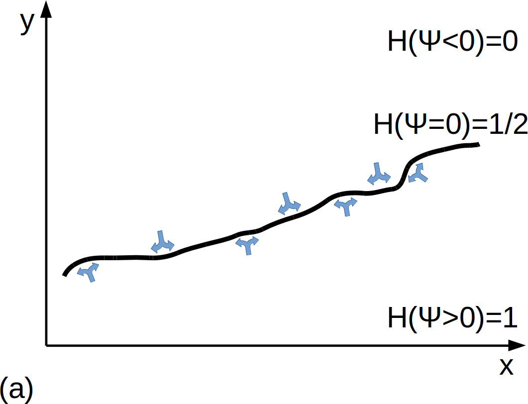
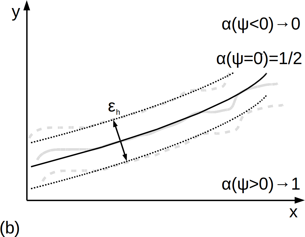
Figure 1: Schematic picture of an instantaneous sample of the sharp interface disturbed by the field of stochastic forces (a) and its ensemble averaged counterpart (b). In the case (a) $\epsilon_{h}\!=\!0$, in the case (b) $\epsilon_{h}>0$.

If all details of the sharp interface evolution in Fig. 1(a) are accounted for, then $\mathbf{w}\!=\!\mathbf{W}$, $\psi\!=\!\Psi$, $\epsilon_{h}\!=\!0$. Hence, the Heaviside function $H\left(\Psi\right)$ is interpreted as the cumulative distribution function (c.d.f.) and its derivative: the exact Dirac delta function $\delta\left(\Psi\right)$, as the probability density function (p.d.f.) of finding the instantaneous position of the sharp interface. Fig. 1(b) schematically shows during the averaging process some information about a fine structure of the interface is lost, it must be reconstructed by the appropriate model.

Let now apply averaging defined by Eq. (12) to Eq. (1). During the ensemble averaging, $\mathbf{W}$ is decomposed into the sum of its mean $\langle\mathbf{W}\rangle$ and fluctuation $\mathbf{W}^{\prime}$, hence, the ensemble averaged Eq. (1) can be written in the general form as

$$\frac{\partial\alpha}{\partial t}+\mathbf{w}\nabla\alpha=-\langle\mathbf{W}^{\prime}\nabla H\rangle=-\langle\mathbf{W}^{\prime}\!\cdot\!\mathbf{n}_{\Gamma}\delta\left(\Psi\right)\rangle,$$ (13)

where $\nabla H\!=\!\delta\left(\Psi\right)\mathbf{n}_{\Gamma}$, $\mathbf{n}_{\Gamma}\!=\!\nabla\Psi/|\nabla\Psi|$ and we use notation: $\langle\mathbf{W}\rangle\!=\!\mathbf{w}$, $\langle H\rangle\!=\!\alpha$. To derive Eq. (13) it is assumed the fluid phase and its vapor are incompressible, leading to the condition $\nabla\!\cdot\!\mathbf{W}\!=\!0$.

The RHS term in Eq. (13) represents a non-zero correlation between the velocity fluctuation in the direction normal to the sharp interface $\mathbf{W}^{\prime}\!\cdot\!\mathbf{n}_{\Gamma}$ and its instantaneous position indicated by the Dirac’s delta function $\delta\left(\Psi\right)$. This term is closed by the approach introduced by Wacławczyk and Oberlack [2011] for modeling of the interaction between stratified flows and turbulence. Therein, application of the eddy diffusivity model and ensemble averaging allows to model the RHS in Eq. (13) by the sum of diffusion and counter gradient diffusion, where the latter term is closed using the non-conservative model. This leads to $\alpha\left(\mathbf{x},t\right)$ represented by the normal distribution as it was suggested by Brocchini and Peregrine [2001a, b] in the context of the interfaces agitated by the turbulent eddies. An alternative approach used by Wacławczyk and Wacławczyk [2015], is the conservative closure of the counter gradient diffusion term: $-\nabla\cdot\left[C\alpha\left(1-\alpha\right)\mathbf{n}_{\Gamma}\right]$, $\mathbf{n}_{\Gamma}\!=\!\nabla\psi/|\nabla\psi|$; after separation of advection and re-initialization in Eq. (13) this latter assumption allows to derive Eq. (9) and Eq. (5), respectively.

In works of Wacławczyk et al. [2014] and Wacławczyk and Wacławczyk [2015], the coefficients $D\left(\mathbf{x},t\right)$, $C\left(\mathbf{x},t\right)$ in Eq. (5) are related to local properties of the ensemble averaged turbulent velocity field. In the present work, we assume $D\!=\!C\epsilon_{h}$ where $C\!=\!const.$, $\epsilon_{h}\!=\!const.$, hence, the discussed conservative closure of the counter gradient diffusion leading to Eq. (5) results in the probability $\alpha\left(\psi\right)$ defined in terms of the logistic distribution, where, the c.d.f. $\alpha\left(\psi\right)$ is given by Eq. (6) and p.d.f. by $\tilde{\delta}\left(\alpha\right)/\epsilon_{h}$ in Eq. (8). The scale parameter $\epsilon_{h}>0$ in these equations is related to the standard deviation $d=\epsilon_{h}\pi/\sqrt{3}\,[m]$. Moreover, the mapping between $\alpha\left(\psi\right)-\psi\left(\alpha\right)$ given by Eq. (7) is the quantile function of the logistic distribution with the expected value equal to zero, see Balakrishnan [1992].

For aforementioned reasons, the zero level-set of the signed-distance function $\psi\left(\alpha\!=\!1/2\right)\!=\!0$ describes the expected position of the regularized interface and $\alpha\left(\psi\!=\!0\right)\!=\!1/2$ indicates the probability with which one of the two phases sharing the regularized interface can be found. One notices, the sum of probabilities of finding the phase one or finding the phase two in every point of the considered domain: $\alpha_{1}+\alpha_{2}=1$ is a conserved quantity. This picture of the averaged or regularized interface is schematically presented in Fig. 1(b).

In Sec. 1, the relation between the SLS and VOF sharp interface models has been discussed, see description of Eqs. (9)-(11). Next, we will show that Eq. (10) is the conservative form of modified Allen-Cahn phase field model given by Eq. (4). This observation permits the physical interpretation of re-initialization in the level-set methods and introduces the phase field model with the order parameter that is a conserved quantity.

2.2 Conservative phase field model of the non-flat, regularized interface

In order to show the model given by Eqs. (9) and (10) describes the evolution of non-flat regularized interface in the state of phase equilibrium, in the present paper the relation between Eq. (10) and modified Eq. (4) is established. To derive it, we use Eq. (8), and Eq. (5) in the non-conservative form to arrive at

$$\frac{\partial\alpha}{\partial\tau}=\frac{C}{\epsilon_{h}}\left[\epsilon_{h}^{2}\nabla^{2}{\alpha}-\left(1-2\alpha\right)\alpha\left(1-\alpha\right)|\nabla\psi|+\epsilon_{h}\alpha\left(1-\alpha\right)\kappa\right],$$ (14)

where $\kappa\!=\!-\nabla\cdot\mathbf{n}_{\Gamma}$ and $\mathbf{n}_{\Gamma}\!=\!\nabla\psi/\nabla\psi$. If $\alpha\left(\psi\right)$ is given by Eq. (1) then $|\nabla\psi\left(\alpha\right)|\!=\!1$ in Eq. (14) and hence, the first two terms on the RHS of Eq. (14) are identical to the RHS terms in Eq. (4).

The Allen-Cahn equation (4) is obtained by computation of the functional derivative of the Ginzburg-Landau functional representing the interfacial density of the Helmholtz free energy

$$F\!\left[\alpha\right]=\int_{V}\sigma\left[\epsilon_{h}^{2}|\nabla\alpha|^{2}+f\left(\alpha\right)\right]dV,$$ (15)

where $\sigma$ is a constant with dimension $[J/m^{2}]$ (see Allen and Cahn [1979], Anderson et al. [1998], Moelans et al. [2008], Kim et al. [2014]). The contribution from the term accounting for the interface deformation, to the best of this author’s knowledge, is absent in the definitions of the Ginzburg-Landau functional known in the literature (see e.g. Cahn and Hilliard [1958], Allen and Cahn [1979], Anderson et al. [1998], Yue et al. [2007], Brassel and Bretin [2011], Kim et al. [2014], Pashos et al. [2015], Fedeli [2017]). We recall after Allen and Cahn [1979] the original form of the Ginzburg-Landau functional given by Eq. (15) is equivalent to the van der Waals [1979] density based functional derived only for the flat interfaces.

As a consequence of Eqs. (14) and (15) in the present paper it is proposed to add the new term to the RHS of Eq. (15). This term, further denoted as $k\left(\alpha\right)$ has to satisfy the relation

$$\int_{V}\frac{\sigma}{2\epsilon_{h}}\,\frac{\partial k}{\partial\alpha}dV\deltaup\alpha=-\int_{V}\sigma\,\alpha\left(1-\alpha\right)/\epsilon_{h}\kappa\,dV\deltaup\alpha.$$ (16)

Next, we show the presence of the new term in the interfacial energy density balance is essential to guarantee the state of phase equilibrium of the non-flat interface. As the functional derivative of $k\left(\alpha\right)$ given by Eq. (16), resembles the capillary term: $\sigma\tilde{\delta}\left(\alpha\right)/\epsilon_{h}|\nabla\psi|\mathbf{n}_{\Gamma}\kappa=\sigma\nabla\alpha\kappa$ added to the momentum balance in the one-fluid formulation exploiting the sharp interface model, the new term may be interpreted as contribution to the total interfacial energy density from the energy required to deform the flat interface.

The contribution to interfacial energy density due to geometrical deformation of the system is absent in Eq. (15), for this reason, the modified Ginzburg-Landau functional reads

$$F_{k}\!\left[\alpha\right]=\int_{V}\sigma\left[\epsilon_{h}^{2}|\nabla\alpha|^{2}+f\left(\alpha\right)+\epsilon_{h}k\left(\alpha\right)\right]dV.$$ (17)

If we assume that at the boundaries of the domain of interest characterized by the normal vector $\mathbf{n}$ the condition $\nabla\alpha\!\cdot\!\mathbf{n}\!=\!0$ is satisfied, the variation of $F_{k}\!\left[\alpha\right]$ is obtained in the form

$$\deltaup F_{k}\!\left[\alpha\right]=\int_{V}\sigma\left[-2\,\epsilon_{h}^{2}\nabla^{2}\alpha+2\,\alpha\left(1-\alpha\right)\left(1-2\alpha\right)+\epsilon_{h}\frac{\partial k}{\partial\alpha}\right]dV\deltaup\alpha=0,$$ (18)

as we search for the minimum of $F_{k}\!\left[\alpha\right]$ with the respect to $\alpha\left(\psi\right)$. Since the volume integral in Eq. (17) is calculated over arbitrary $V$, the only way Eq. (18) is equal to zero, is that

$$\sigma\left[\nabla^{2}\alpha-\alpha\left(1-\alpha\right)\left(1-2\alpha\right)/\epsilon_{h}^{2}-\frac{1}{2\epsilon_{h}}\frac{\partial k}{\partial\alpha}\right]=0.$$ (19)

As it was pointed out above in Eq. (16), Eq. (14) predicts

$$\frac{\sigma}{2\epsilon_{h}}\frac{\partial k}{\partial\alpha}=\sigma\alpha\left(1-\alpha\right)/\epsilon_{h}\nabla\cdot\left(\frac{\nabla\alpha}{|\nabla\alpha|}\right),$$ (20)

where we used $\kappa=-\nabla\cdot\left(\nabla\alpha/|\nabla\alpha|\right)$. After rearrangement of terms in Eq. (20) with the help of Eq. (8), using the property of the signed distance function $|\nabla\psi\left(\alpha\right)|=1$, the following formula is obtained

$$\frac{\sigma}{2\epsilon_{h}}\frac{\partial k}{\partial\alpha}=\sigma\left[\nabla^{2}\alpha-\alpha\left(1-\alpha\right)\left(1-2\alpha\right)/\epsilon_{h}^{2}\right].$$ (21)

Substitution of Eq. (21) into Eq. (18) or Eq. (19) leads to the condition of the phase equilibrium; the functional derivative of the modified Ginzburg-Landau functional $F_{k}\!\left[\alpha\right]$ representing the chemical potential, is equal to zero

$$\frac{\deltaup F_{k}\!\left[\alpha\right]}{\deltaup\alpha}=0.$$ (22)

Thus, $F_{k}\!\left[\alpha\right]$ has the extremum when $\alpha\left(\psi\right)$ is given by Eq. (1) or equivalently $|\nabla\psi\left(\alpha\right)|\!=\!1$. Later in this paper, we will argue using results of numerical simulations Eq. (22) provides the condition required for existence of the $F_{k}\!\left[\alpha\right]$ minimum, up to this moment, we assume that this case is met. In the following section it is shown how condition given by Eq. (22) can be interpreted.

2.3 Velocity of the regularized interface

Subsequently, it is demonstrated that physical interpretation of functions $\alpha\left(\psi\right)-\psi\left(\alpha\right)$ and their re-initialization equation (10) postulated in Sec. 2.1 and Sec. 2.2 is plausible; using again Eq. (8) to eliminate $\nabla\alpha$ from Eq. (14), we arrive at

$$\frac{\partial\psi}{\partial\tau}=C\left\{\left(1-2\alpha\right)\left[\left(\nabla\psi\right)^{2}-|\nabla\psi|\right]+\epsilon_{h}\left[\nabla^{2}{\psi}-\nabla\!\cdot\!\left(\frac{\nabla\alpha}{|\nabla\alpha|}\right)\right]\right\},$$ (23)

where the two terms on the RHS are equal to zero only when the mapping between $\alpha\left(\psi\right)\!-\!\psi\left(\alpha\right)$ is possible. Eq. (23) may be interpreted as the formula for the normal velocity component $\mathbf{w}\left(\psi\right)\cdot\mathbf{n}_{\Gamma}$ of the expected interface position $\psi\left(\alpha=1/2\right)=0$ as $\partial\psi/\partial\tau\,[m/s]$. If the interface is in the state of phase equilibrium, then, the RHS of Eq. (23) and thus the normal velocity component of the expected interface position is equal to zero. Let us notice, the first RHS term acts only away from the interface, therefore, when $\alpha\left(\psi\!=\!0\right)\!=\!1/2$ only the second RHS term in Eq. (23) affects the velocity $\partial\psi/\partial\tau\,[m/s]$. This result agrees with the prediction of Allen and Cahn [1979] showing the normal component of the interface velocity is proportional to the interface curvature.

As in the phase field interface models based on Eq. (15) the term $k\left(\alpha\right)$ is absent in the interfacial energy density functional, spontaneous loss or gain of mass due to non-zero velocity $\mathbf{w}\left(\psi\right)\!\cdot\!\mathbf{n}_{\Gamma}\!=\!\partial\psi/\partial\tau$ may be the consequence. Such artificial phenomenon is described in details by Yue et al. [2007] and was confirmed by Bao et al. [2012] in the case of simulations with the Cahn-Hilliard equation derived based on the original form of the Ginzburg-Landau functional given by Eq. (15). The main mechanism of this spurious phase transition is the flow of energy between the first and the second RHS terms in Eq. (15). As it is explained by Yue et al. [2007] “this flow is perfectly permissible within Cahn-Hilliard framework but would violate mass conservation for the drop”. The modified functional $F_{k}\!\left[\alpha\right]$ given by Eq. (17) guarantees satisfaction of the law of mass conservation as its functional derivative is always, exactly equal to zero if $\alpha\left(\psi\right)$ is given by Eq. (1) and hence $|\nabla\psi\left(\alpha\right)|\!=\!1$.

3 Numerical solution of the model equations

As it was mentioned during interpretation of Eq. (23), incorrect numerical solution of Eq. (10) can cause the spurious phase transition leading to the artificial decay or gain of mass. In Sec. 3 we have shown Eq. (10) guarantees satisfaction of the condition given by Eq. (22) required for the phase equilibrium, therefore, the main challenge for the numerical schemes is to keep this balance of interfacial energies unchanged.

If the interfacial energy density is away from its minimum because $\alpha\left(\psi\right)$ is not given by Eq. (1), for instance due to artificial deformation caused by the numerical errors, the robust numerical scheme must be able to overcome this departure from the equilibrium state and, after some re-initialization steps, assure satisfaction of the condition given by Eq. (22). This is possible only if Eq. (22) provides the condition for the minimum of the modified energy functional $F_{k}\left[\alpha\right]$ given by Eq. (17). In the case Eq. (22) provides the condition for existence of the maximum of $F_{k}\left[\alpha\right]$, the divergence of the numerical solution would be the expected consequence of any departure from the equilibrium state.

In this section, we discuss two numerical techniques allowing to minimize impact of the discretization errors on the numerical solution of Eqs. (9) and (10). The main prerequisites for the remaining part of this paper are: the velocity $C\!=\!1\,[m/s]$ and the width of the interface is $\epsilon_{h}\!=\!\sqrt{K}\Delta x/4\,[m]$, $K=1,2$ are kept constant. The second-order accurate finite volume method is used for spatial discretization of Eqs. (9) and (10). If it is not stated otherwise, Eq. (9) is advanced in time using the second order accurate implicit Euler scheme (TTL) (see Ferziger and Perić [2002], Schäfer [2006]). The stationary solution of re-initialization Eq. (10) in time $\tau\,[s]$ is obtained using the third-order accurate TVD Runge-Kutta method introduced by Gottlieb and Shu [1998].

At first, the constrained interpolation is introduced to improve accuracy of approximation of the RHS fluxes in Eq. (10). Afterwards, in order to avoid errors introduced by the second-order accurate flux limiters, the new semi-analytical Lagrangian scheme for discretization of Eq. (9) is put forward. The new schemes for the numerical solution of Eqs. (9) and (10) provide means to obtain the third-order convergence rate of advection and re-initialization in time, and second-order convergence rate of the interface shape (volume) and curvature. These temporal and spatial convergence rates are the same as theoretical orders of accuracy of the numerical schemes used to approximate Eqs. (9) and (10).

3.1 Constrained interpolation

In what follows we show how to exploit relation between $\alpha\left(\psi\right)-\psi\left(\alpha\right)$ during numerical solution of Eq. (10). In particular, the constrained interpolation scheme (CIS) introduced in this section is used to approximate the RHS fluxes in Eq. (10), see also B. This scheme permits to use the steep profile of the hyperbolic tangent with the disretization errors typical for interpolation of linear functions.

The idea of CIS is based on a simple observation. Since the mapping between $\alpha\left(\psi\right)-\psi\left(\alpha\right)$ is possible, then, instead interpolating $\alpha_{f}$ directly (subscript $f$ denotes the value interpolated to the face $f$ of the given control volume $P$), we can interpolate $\psi_{f}$ and afterwards calculate $\alpha_{f}\!=\!\alpha\left(\psi_{f}\right)$ using the profile given by Eq. (6) as a constraint. In the case of simplest linear interpolation of $\psi_{f}$ the constrained interpolation is summarized below

$$\begin{split}\psi_{f}&\approx\frac{1}{2}\left(\psi_{P}+\psi_{F}\right)+\mathcal{O}\left(\Delta x^{2}\right),\\ \alpha_{f}&=\alpha\left(\psi_{f}\right)=\frac{1}{1+\exp{\left(-\psi_{f}/\epsilon_{h}\right)}},\end{split}$$ (24)

where subscripts $F,f,P$ denote the neighbor control volume $F$ and face $f$ of the given control volume $P$, respectively. One notices, no approximation is needed to compute $\alpha_{f}$ in Eqs. (24), the numerical error of the constrained interpolation scheme is introduced only during the linear interpolation used to obtain $\psi_{f}$. It is almost immediately clear from Eqs. (24) the constrained computation of $\tilde{\delta}\left(\alpha\right)\!=\!\alpha\left(1-\alpha\right)$ in Eq. (10) should be less prone to the dispersive errors introduced when the linear interpolation (LIS) is used directly to compute $\alpha_{f}$. In what follows, we provide quantitative arguments for the above statement.

To investigate properties of the constrained interpolation, re-initialization of the one-dimensional regularized Heaviside function is studied in the computational domain $\Omega=<\!0,1\!>\,[m]$. The interface $\Gamma$ is located at $x_{\Gamma}=0.6\,[m]$ to avoid symmetry between the uniform grid nodes distribution and re-initialized profile of hyperbolic tangent; $\Delta x=1/N_{c}$ where $N_{c}=128$ is the number of control volumes. At all boundaries of the computational domain $\Omega$, the Neumann boundary condition for $\alpha\left(\psi\right)$ is used.

In order to compare the constrained interpolation scheme (CIS) with the second-order accurate linear interpolation scheme (LIS) two tests are performed. In the first test, the initial support of $\alpha\left(\psi\right)$ profile is four times smaller than in the final profile where $\epsilon_{h}=\Delta x$; in this test the diffusion causes widening of the interface.

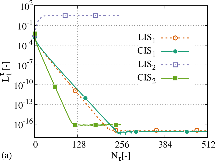
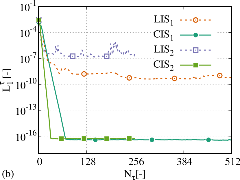
Figure 2: Convergence of the solutions to the diffusion (a), and compression (b) dominated test problems, $L_{1}^{\tau}$ denotes norm defined by Eq. (31). In both tests the linear interpolation (LIS) or constrained interpolation (CIS) are used, subscripts $1,2$ denote simulation with time steps: $\Delta\tau_{1}=\Delta x/4$, $\Delta\tau_{2}=2\Delta\tau_{1}$. Results in Figs. 3 – 5 were evaluated at the end of the re-initialization process after $N_{\tau}=256$ or $N_{\tau}=512$ re-initialization steps, respectively; only the convergent results are illustrated therein.

In the second test case, the initial support of $\alpha\left(\psi\right)$ profile is four times wider than the final one, where $\epsilon_{h}=\Delta x/4$. Here, the counter-gradient diffusion leads to reduction of the interface thickness. To closely inspect sensitivity of the solution on the re-initialization time step size, solutions of Eq. (10) obtained with the two time step sizes $\Delta\tau_{1}=\Delta x/4$ and $\Delta\tau_{2}=2\Delta\tau_{1}$ are compared. In the case $\Delta\tau_{1}$ and $\Delta\tau_{2}$, $N_{\tau}^{1}=512$ and $N_{\tau}^{2}=256$ re-initialization steps are carried out, respectively, to assure the same total re-initialization time.

The results presented in Fig. 2, illustrate convergence of the re-initialization equation (10) in time $\tau$ visualized using the $L_{1}^{\tau}$ norm defined by Eq. (31). These results were obtained with the LIS or CIS interpolation and two time steps $\Delta\tau_{1},\,\Delta\tau_{2}$ denoted using subscripts $1,2$, respectively. We note, usage of the larger time step $\Delta\tau_{2}=2\Delta\tau_{1}$ with LIS leads to divergence of the simulation results in the case dominated by the diffusion, see Fig. 2(a). In the compression dominated case, the accuracy of the solution obtained with the time steps $\Delta\tau_{k}$, $k=1,2$ and LIS is lower than this with CIS. At the same time, the convergence rates and levels of accuracy obtained with CIS seem to be only slightly affected by the selected time step size $\Delta\tau_{k}$, $k=1,2$, compare results in Fig. 2(a)(b). When CIS is used in both test cases, the machine accuracy is achieved independent from the time step size chosen; compare results obtained with CIS (solid lines, solid symbols) and LIS (dashed lines, hollow symbols) depicted in Fig. 2(a)-(b).

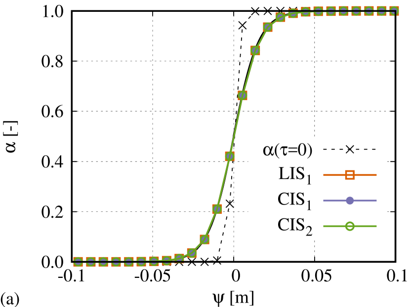
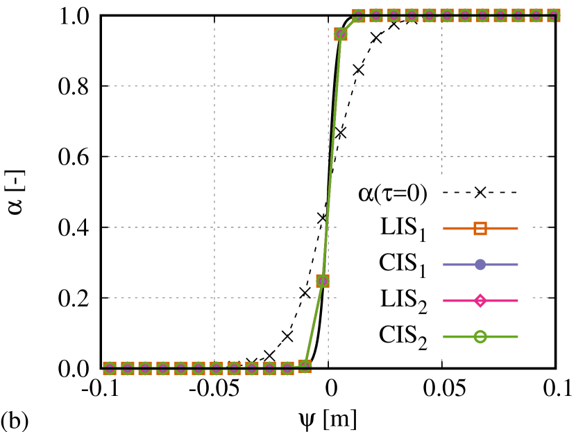
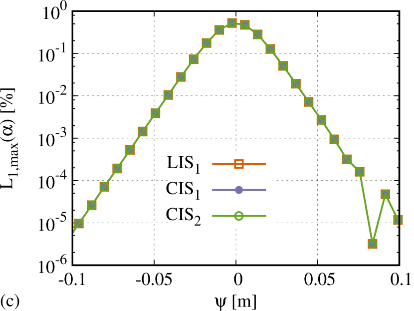
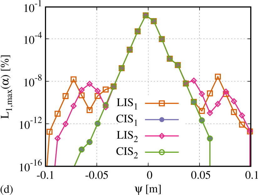
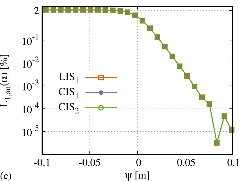
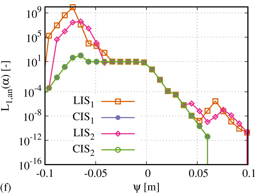
Figure 3: The comparison of $\alpha\left(\psi\right)$ profiles reconstructed with the LIS, CIS interpolation during the diffusion (left) and compression (right) dominated test cases from Fig. 2. In diagrams (a),(b) numerical results are compared with the analytic solution (black solid line), diagrams (c)-(f) depict corresponding errors defined by Eqs. (32) and (33); subscripts $1,2$ denote simulations with $\Delta\tau_{1}=\Delta x/4$, $\Delta\tau_{2}=2\Delta\tau_{1}$.

The convergence of the re-initialization process with two different interpolation schemes LIS or CIS is reflected in distribution of the numerical errors after it is ceased. These errors are obtained by the comparison of the numerical solution with the known analytical profiles of $\alpha\left(\psi\right)$ given by Eq. (6) and the first components of its first/second-order spatial derivatives. Figs. 3 – 5 illustrate these profiles as well as the errors of LIS and CIS interpolation schemes using the $L_{1,an}$ and $L_{1,max}$ norms defined by Eqs. (32) and (33). All results depicted in Figs. 3 – 5 were evaluated at the end of the re-initialization process, only the convergent results from Fig. 2 have been illustrated therein.

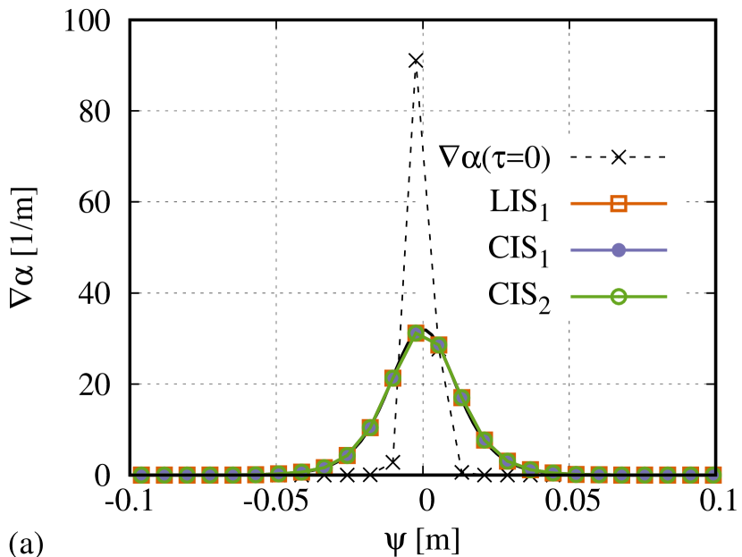
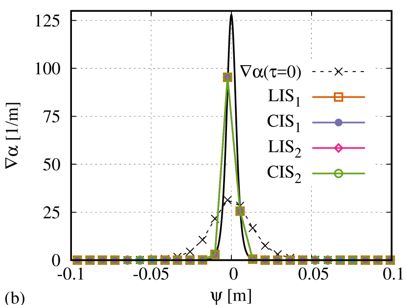
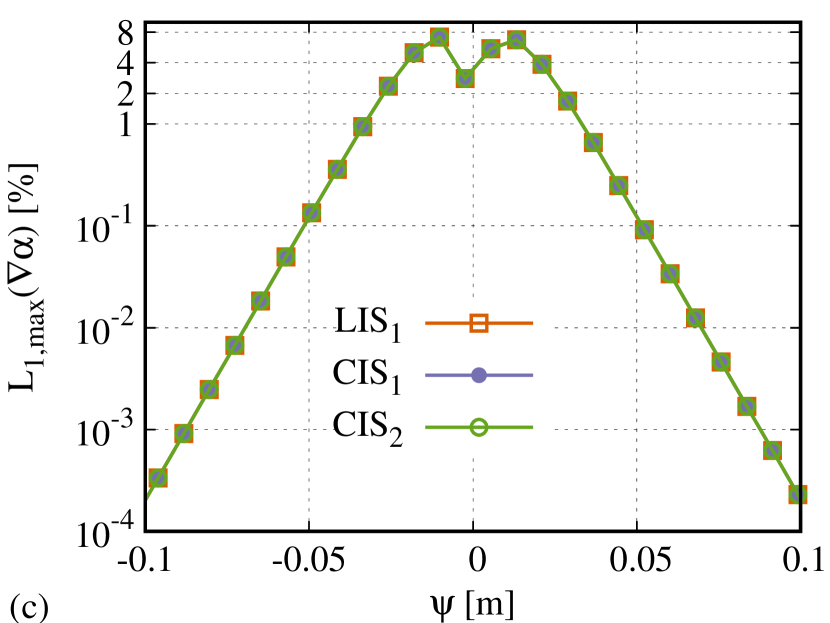
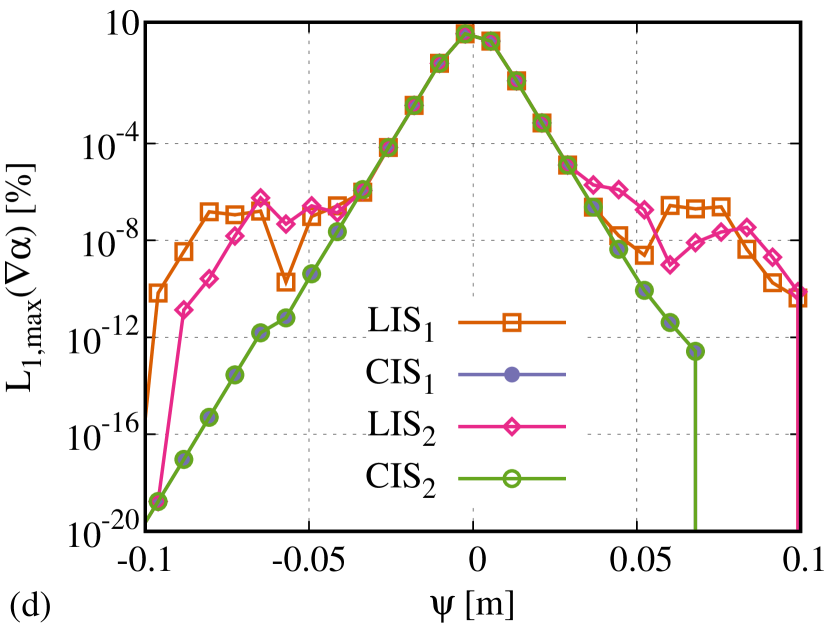
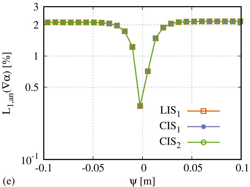
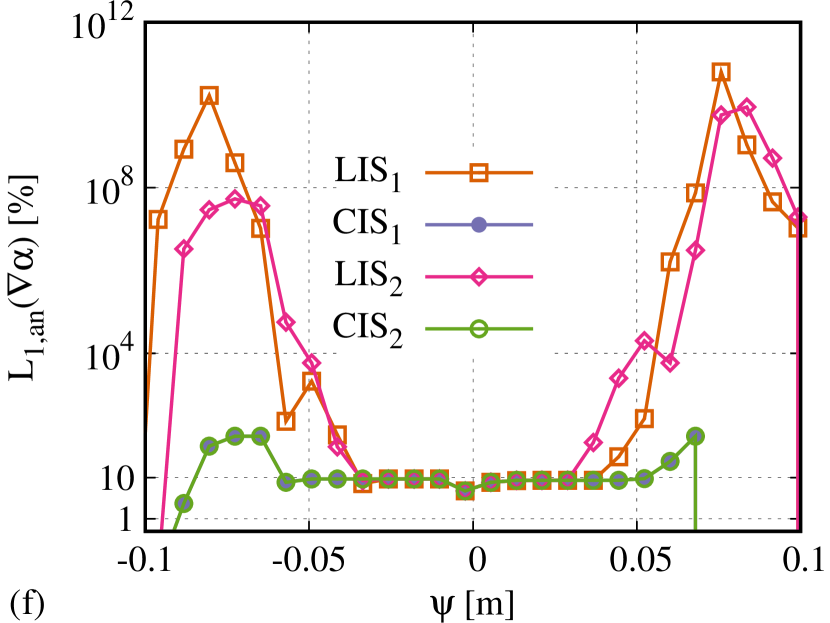
Figure 4: The comparison of the first component of $\nabla\alpha\left(\psi\right)$ reconstructed with the LIS, CIS interpolation during the diffusion (left) and compression (right) dominated test cases from Fig. 2. In diagrams (a),(b) numerical results are compared with the analytic solution (black solid line), diagrams (c)-(f) depict corresponding errors defined by Eqs. (32) and (33); subscripts $1,2$ denote simulations with $\Delta\tau_{1}=\Delta x/4$, $\Delta\tau_{2}=2\Delta\tau_{1}$.

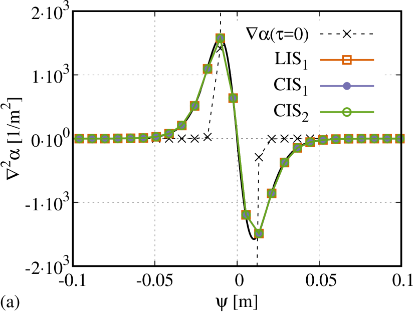
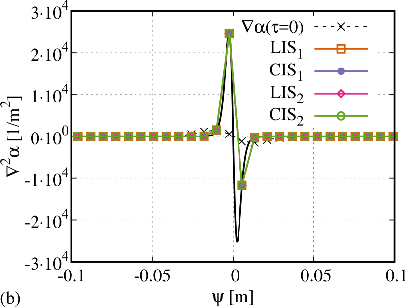
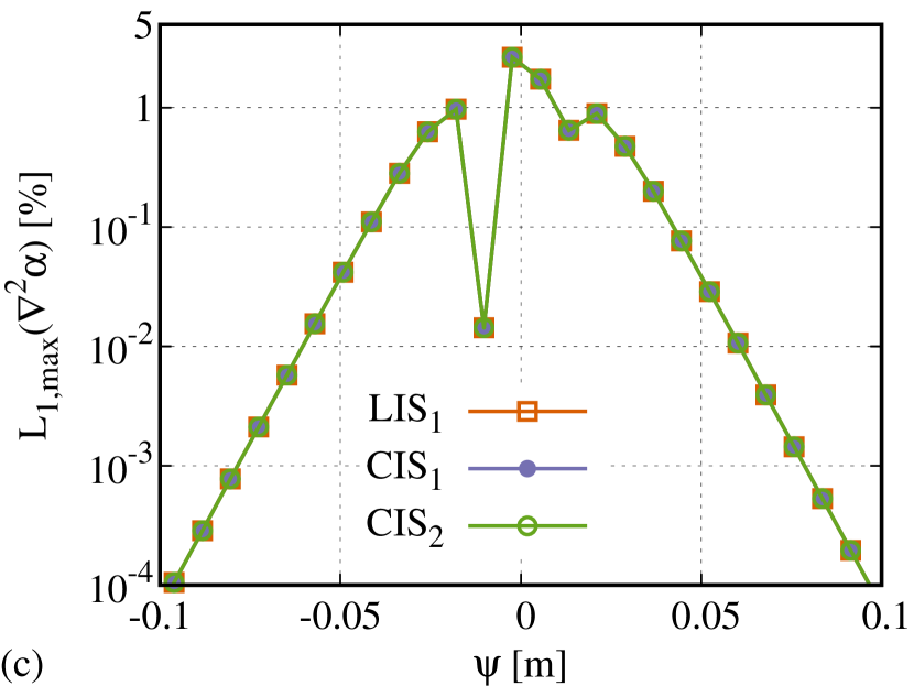
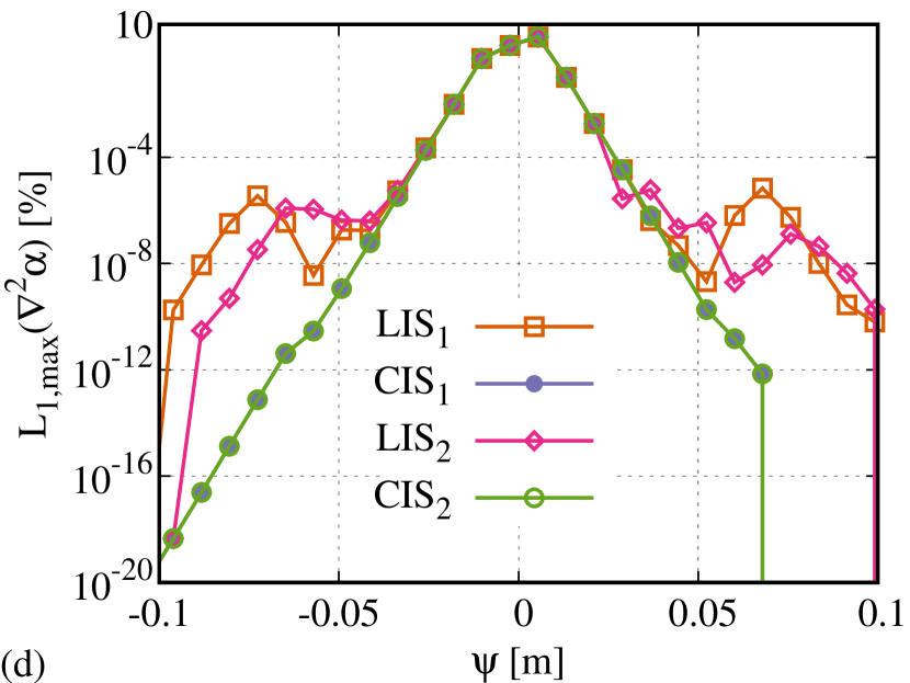
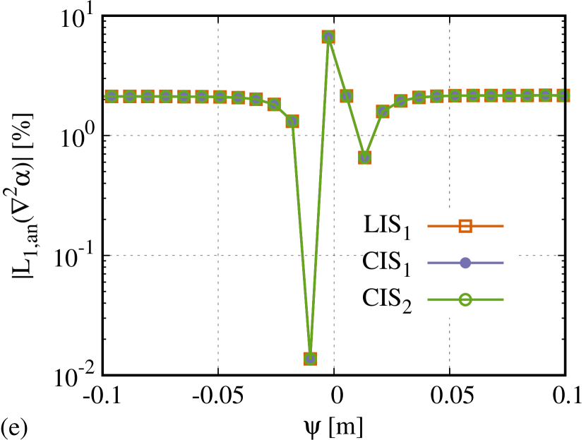
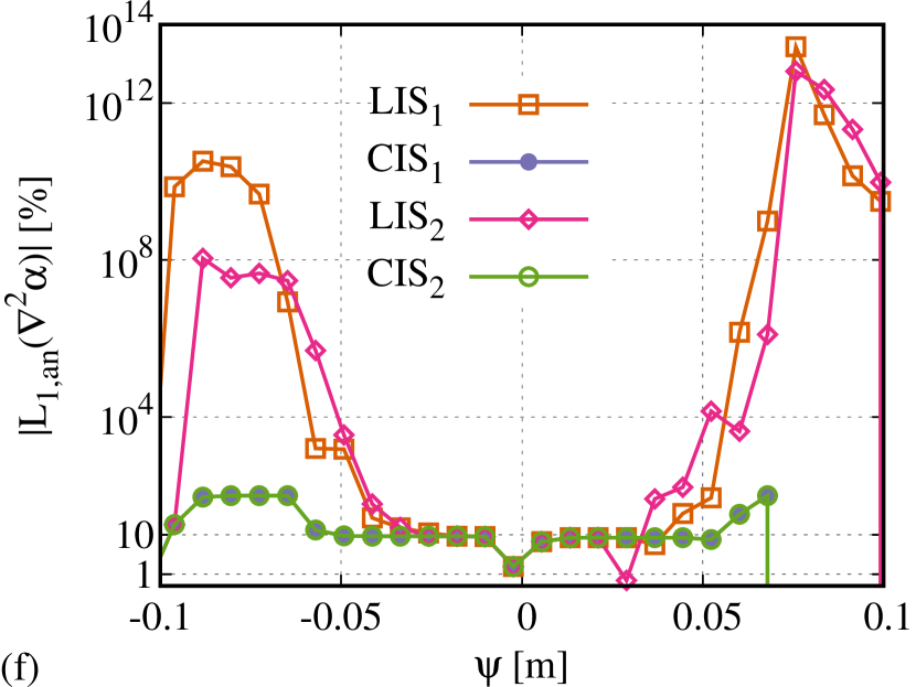
Figure 5: The comparison of the first component of $\nabla^{2}\alpha\left(\psi\right)$ reconstructed with the LIS, CIS interpolation during the diffusion (left) and compression (right) dominated test cases from Fig. 2. In diagrams (a),(b) numerical results are compared with the analytic solution (black solid line), diagrams (c)-(f) depict corresponding errors defined by Eqs. (32) and (33); subscripts $1,2$ denote simulations with $\Delta\tau_{1}=\Delta x/4$, $\Delta\tau_{2}=2\Delta\tau_{1}$.

In the diffusion dominated test case depicted in the left column of Figs. 3 – 5, almost no differences can be observed in the distribution of the errors when LIS or CIS are used to reconstruct $\alpha\left(\psi\right)$, regardless of the selected time step size, see Figs. 3(c)(e)–5(c)(e). This result is expected as the convergence rates of $L^{\tau}_{1}$ norms obtained using $\text{LIS}_{1}$ and $\text{CIS}_{1}$ are almost identical, see Fig. 2(a).

In the compression dominated test case presented in the right column of Figs. 3 – 5, it can be seen the errors in results obtained using CIS are localized in the vicinity of the interface $\psi\left(\alpha=1/2\right)=0$ and they do not exhibit signs of numerical dispersion manifested in the oscillations of the reconstructed solutions and corresponding errors. The behavior of CIS errors is in contrast with the oscillatory results obtained when LIS is used, compare results in Figs. 3(d)(f)–5(d)(f).

As profiles in Figs. 3(c)(d)–5(c)(d) are normalized by maximal value of $\alpha$, $\nabla\alpha$ and $\nabla^{2}\alpha$, respectively, the distributions of the $L_{1,max}$ norm is symmetrical around the expected position of the interface $\psi\left(\alpha\!=\!1/2\right)\!=\!0$. In the case of normalization with the exact $\alpha$, $\nabla\alpha$ or $\nabla^{2}\alpha$ values as it is illustrated in Figs. 3(e)(f)–5(e)(f), the increment of the errors levels defined by the $L_{1,an}$ norm away from the interface $\psi\left(\alpha=1/2\right)=0$ is caused by the division of small numbers $\sim{\mathcal{O}}\left(10^{-12}\right)$ differing by the order of magnitude.

The main difference between both interpolation strategies is the lack of numerical solution and hence errors oscillations when CIS is used. Moreover, results obtained with CIS are less sensitive to the selected time step size $\Delta\tau_{k}$, $k=1,2$ as is shown by the $L_{1}^{\tau}$ recordings depicted in Fig. 2. The difference in the performance of both interpolation schemes is explained by usage of $\alpha\left(\psi\right)$ profile given by Eq. (6) in CIS constraining values interpolated to the faces of the given control volume, see Eqs. (24) and B.

The results presented in Fig. 2 and Figs. 3 – 5 clearly demonstrate advantages of CIS over LIS, therefore, CIS will be preferred for discretization of the RHS fluxes in Eq. (10) in the remaining part of the present paper where the results of simulations with advection of $\alpha\left(\psi\right)$ and $\psi\left(\alpha\right)$ level-set functions are presented.

3.2 Lagrangian advection scheme

In this section, a semi-analytical Lagrangian scheme for discretization of Eq. (9) governing advection of $\alpha\left(\psi\right)-\psi\left(\alpha\right)$ level-set functions in the external velocity field is put forward. The main motivation for its introduction are problems with obtaining the theoretical convergence rates of the re-initialization process and interface curvature on gradually refined grids during advection of the solid objects in the divergence free velocity fields. In particular, when the second-order accurate spatial discretization and third order accurate TVD Runge-Kutta method are used alongside in solution of the advection and re-initialization equations (9)-(10), respectively. In the majority of works where Eq. (9) is solved using the first/second-order accurate spatial discretization authors consider only numerical accuracy (or the convergence rate) of the advected interface shape; plethora of examples is available in the literature see for instance works of Wacławczyk and Koronowicz [2006, 2008a, 2008b], Osher and Fedkiw [2003], Olsson and Kreiss [2005], Chiu and Lin [2011], Balcazar et al. [2014], McCaslin and Desjardins [2014], Wacławczyk [2015]. Moreover, it is hard to find works where detailed information about the convergence rate of re-initialization during advection of the level-set functions $\alpha\left(\psi\right)$ and/or $\psi\left(\alpha\right)$ is presented.

In order to derive a more accurate advection scheme, Eq. (8) is used again this time to obtain the correct numerical solution of Eq. (9). In this regard, the new Lagrangian advection scheme also uses the profile of $\alpha\left(\psi\right)$ as a constraint because it is assumed Eq. (8) holds after each re-initialization cycle. This assumption is reasonable if stationary solution to Eq. (10) is obtained with the smallest possible error, see results in Sec. 3.1 and discussion in Wacławczyk [2015]. After substitution of Eq. (8) into Eq. (9) we arrive at

$$\frac{\partial\alpha}{\partial t}+\frac{\tilde{\delta}\left(\alpha\right)}{\epsilon_{h}}|\nabla\psi|\mathbf{w}\cdot\mathbf{n}_{\Gamma}=0.$$ (25)

The rearrangement of terms in equation (25) leads to

$$\frac{1}{\alpha\left(1-\alpha\right)}\frac{\partial\alpha}{\partial t}=-\frac{1}{\epsilon_{h}}|\nabla\psi|\mathbf{w}\!\cdot\!\mathbf{n}_{\Gamma}.$$ (26)

The left hand side is now integrated between $\alpha^{n}$ and $\alpha^{n+1}$, whereas the right hand side between $t^{n}$ and $t^{n+1}$ to obtain

$$\ln{\left(\frac{\alpha}{1-\alpha}\right)}\Biggr{|}_{\alpha^{n}}^{\alpha^{n+1}}=-\frac{1}{\epsilon_{h}}\int_{t^{n}}^{t^{n+1}}\!\!\!|\nabla\psi|\mathbf{w}\!\cdot\!\mathbf{n}_{\Gamma}dt,$$ (27)

where $n,\,n\!+\!1$ denotes old and new time levels, respectively. Integration given by Eq. (27) allows to derive the following formula for advancement of $\alpha\left(\psi\right)-\psi\left(\alpha\right)$ in time $t$ which is given by the formula

$$\alpha^{n+1}=\frac{\alpha^{n}\exp{\left[I\left(t^{n}\right)\right]}}{1-\alpha^{n}\left(1-\exp{\left[I\left(t^{n}\right)\right]}\right)},$$ (28)

where the RHS integral in Eq. (27) is denoted as $I(t^{n})$. This integral must be approximated by the appropriate quadrature; in the present work we adopt the second-order Adams-Bashforts method leading to

$$I\left(t^{n}\right)\approx-\frac{1}{\epsilon_{h}}\left[\frac{3}{2}f\left(t^{n},\psi^{n}\right)-\frac{1}{2}f\left(t^{n-1},\psi^{n-1}\right)\right]\Delta t,$$ (29)

where $f=|\nabla\psi|\mathbf{n}_{\Gamma}\cdot\mathbf{w}$. The semi-analytical, explicit scheme given by Eqs. (28) and (29) is second-order accurate in time and no spatial discretization of $\alpha\left(\psi\right)$ is needed as it exploits Lagrangian form of Eq. (9). A lack of spatial disretization in the Lagrangian scheme may be an advantage when compared with the second-order TVD MUSCL controlling only the slope of the local solution. However, at the same time the main disadvantage of the Lagrangian scheme is its non-conservative and explicit formulation, see Eq. (25) and Eqs. (28)-(29), respectively.

Subsequently, the properties of the new Lagrangian scheme are compared with the standard second-order TVD MUSCL used to approximate convective term in Eq. (9). The comparison is carried out during advection of the circular interface in the divergence free velocity field $\mathbf{u}\!=\!(u_{1},u_{2})\!=\!V_{0}/L(y-0.5,0.5-x)$ where $V_{0}\!=\!1\,[m/s]$ and $L\!=\!1\,[m]$. In what follows, advection and re-initialization equations (9)-(10) are solved alongside to advance the circular interface without deformation. In such case we set $\mathbf{w}=\mathbf{u}$ in Eq. (9) and hence in Eqs. (28) and (29). The present investigations are performed in quadratic domain $\Omega=<\!0,1\!>\!\times\!<\!0,1\!>\,[m^{2}]$ on four gradually refined grids $m_{k}=2^{4+k}\times 2^{4+k},\,k=2,\ldots,5$ with the uniform grid nodes distribution; the Neumann boundary condition is used at all boundaries of the computational domain $\Omega$. Initially at $t=0$, the center of the circular interface with the radius $R=0.15\,[m]$ is located at the point $(x_{0},y_{0})=(0.65,0.5)\,[m]$. The time step size $\Delta t_{l}$ during solution of Eq. (5) is chosen to satisfy three CFL conditions: $C\!u_{0}\!\approx\!0.35$, $C\!u_{1}\!\approx\!2C\!u_{0}$, $C\!u_{2}\!\approx\!4C\!u_{0}$, where

$$C\!u_{l}=\sum_{f=1}^{n_{b}}max\left\{\frac{\mathbf{u}_{f}\mathbf{S}_{f}\Delta t_{l}}{V_{P}},0\right\}\quad\text{and}\quad l\!=\!0,1,2,$$ (30)

$n_{b}$ denotes the number of neighbor control volumes, $\mathbf{S}_{f}$ is the surface of the control volume’s $P$ face $f$ and $V_{P}$ is the volume of the control volume $P$. The interface width is set to $\epsilon_{h}\!=\!\sqrt{2}\Delta x/4$ and $\Delta\tau\!=\!D/C^{2}\!=\!\epsilon_{h}$ similarly to the advection tests performed by Wacławczyk [2015].

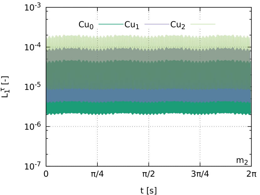
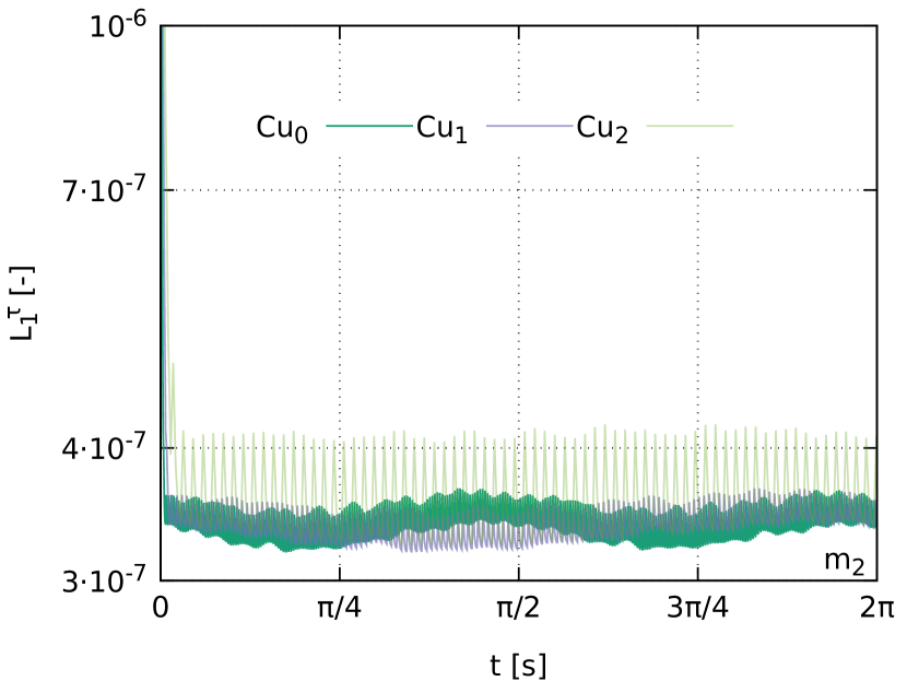
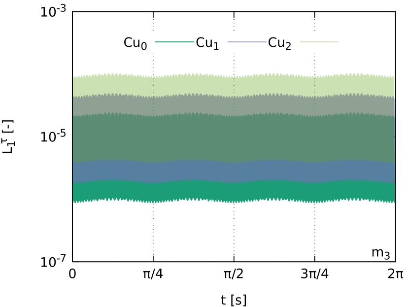
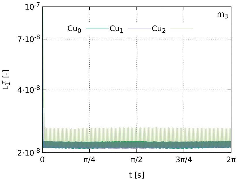
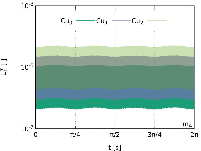
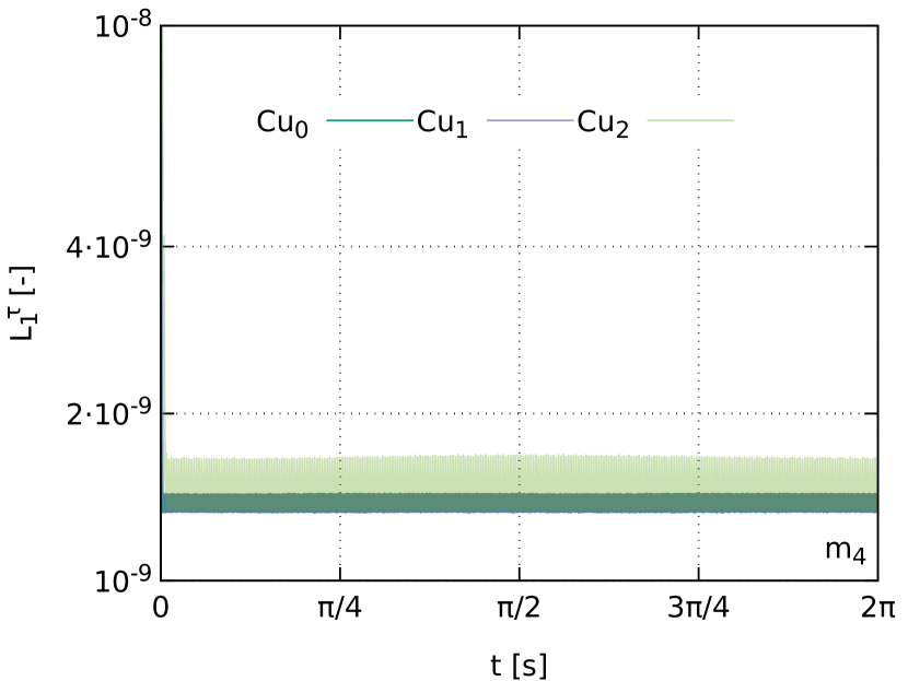
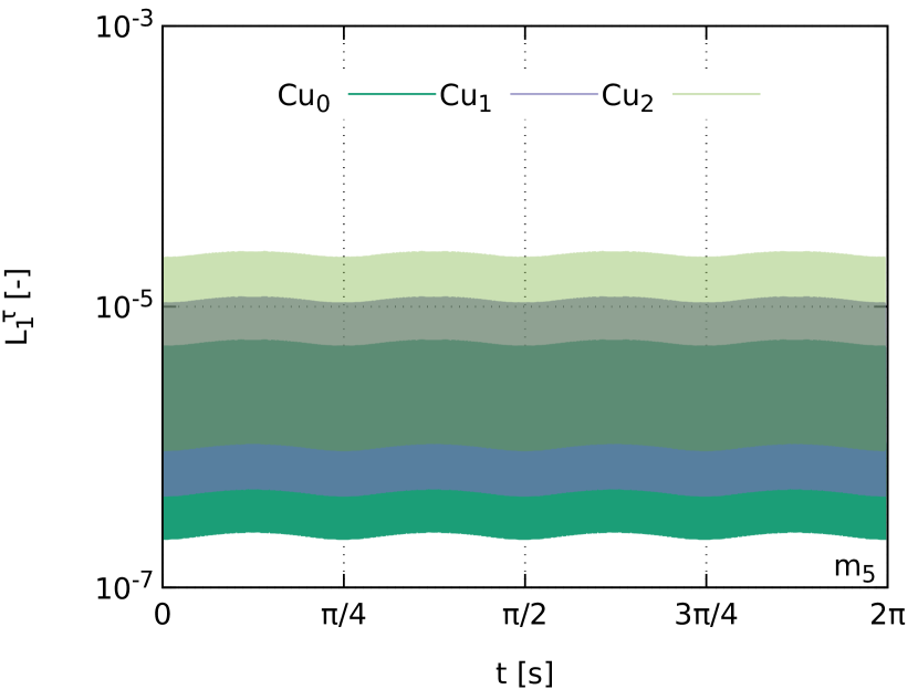
Figure 6: The convergence of advection and re-initialization Eqs. (9) and (10) during advection of the circular interface, $L_{1}^{\tau}$ norm defined by Eq. (31) where $N_{\tau}=4$ steps $\Delta\tau$ is plotted after each time step $\Delta t_{l}$ or $C\!u_{l}$ number $l\!=\!0,1,2$, on four gradually refined grids $m_{k}=2^{4+k}\times 2^{4+k},\,k=2,\ldots,5$ (from top to bottom). The Eulerian (left) or Lagrangian (right) schemes were used to discretize Eq. (9).

Fig. 6 depicts histories of joint convergence of Eqs. (9) and (10) during one revolution of the circular interface. The joint convergence of the advection and re-initialization equations is illustrated using the $L_{1}^{\tau}$ norm plotted after each time step $\Delta t_{l}$, $l\!=\!0,1,2$ during a single re-initialization cycle with $N_{\tau}\!=\!4$ steps $\Delta\tau$. The results in the left column of Fig. 6 are obtained using the implicit Eulerian scheme whereas the results in the right column are obtained with the explicit Lagrangian scheme introduced by Eqs. (28) and (29).

One notices, the diagrams in the right column of Fig. 6, illustrate reduction of the $L_{1}^{\tau}$ norms by the order of magnitude on each subsequent grid $m_{k}$, $k\!=\!2,\ldots,5$, (figures from top to bottom) indicating convergence of the re-initialization process with the gradual grid refinement. In this case, the influence of time step size $\Delta t_{l}$, $l\!=\!0,1,2$ on the convergence rate and error level is minor. The influence of the time step size $\Delta t_{l}$ on the $L_{1}^{\tau}$ norms levels is more evident in the case when Eulerian scheme is used, compare convergence recordings in the left column of Fig. 6. Unlike in the case of Lagrangian scheme, convergence of the solution to Eqs. (9) and (10) with the mesh refinement is disputable when the Eulerian scheme is used to advance Eq. (9) in time $t$. Some reduction in the error levels obtained for different meshes $m_{k}$, $k\!=\!2,\ldots,5$ can be observed in Fig. 6(left), however it does not display the expected second-order accuracy.

We note, in the case of Lagrangian scheme at the beginning of advection several iterations are needed to achieve constant levels of convergence, see for example Fig. 6(right) for grid $m_{2}$. Hence, the net spatial and temporal discretization error introduced by the Lagrangian scheme in Eq. (9) is further reduced by the third-order TVD Runge-Kutta and CIS schemes used in discretization of Eq. (10). This is in contrast to the results obtained using the Eulerian scheme, where the re-initialization step does not reduce errors introduced during advection. The one re-initialization cycle with $N_{\tau}=4$ steps $\Delta\tau$ reduces this error by one order of magnitude but at the beginning of the new re-initialization cycle the error returns back to its previous levels, see left column in Fig. 6. This behavior can be attributed to the errors introduced by the TVD MUSCL advection scheme deforming the interface shape and is the main cause of much slower convergence with the gradual mesh refinement in the case of Eulerian scheme. In the case of the Lagrangian scheme, the error variation during a one re-initialization cycle on the single time step $\Delta t$ remains almost constant. This statement is true for all $C\!u_{l}$, $l\!=\!0,1,2$; we emphasize, exactly the same discretization of Eq. (10) is used when the Eulerian or Lagrangian schemes are used to approximate Eq. (9).

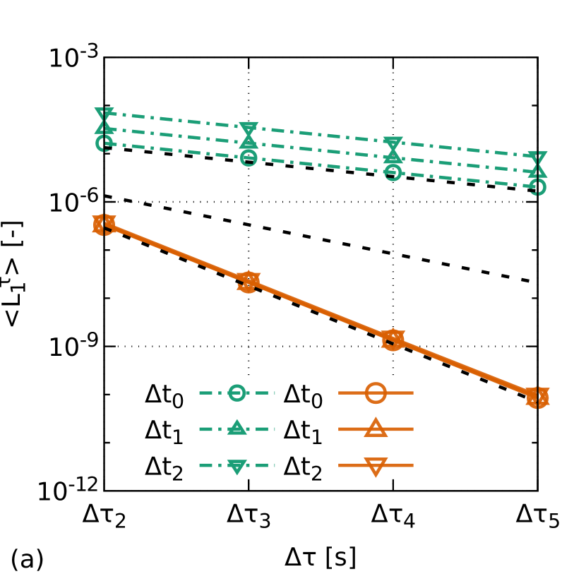
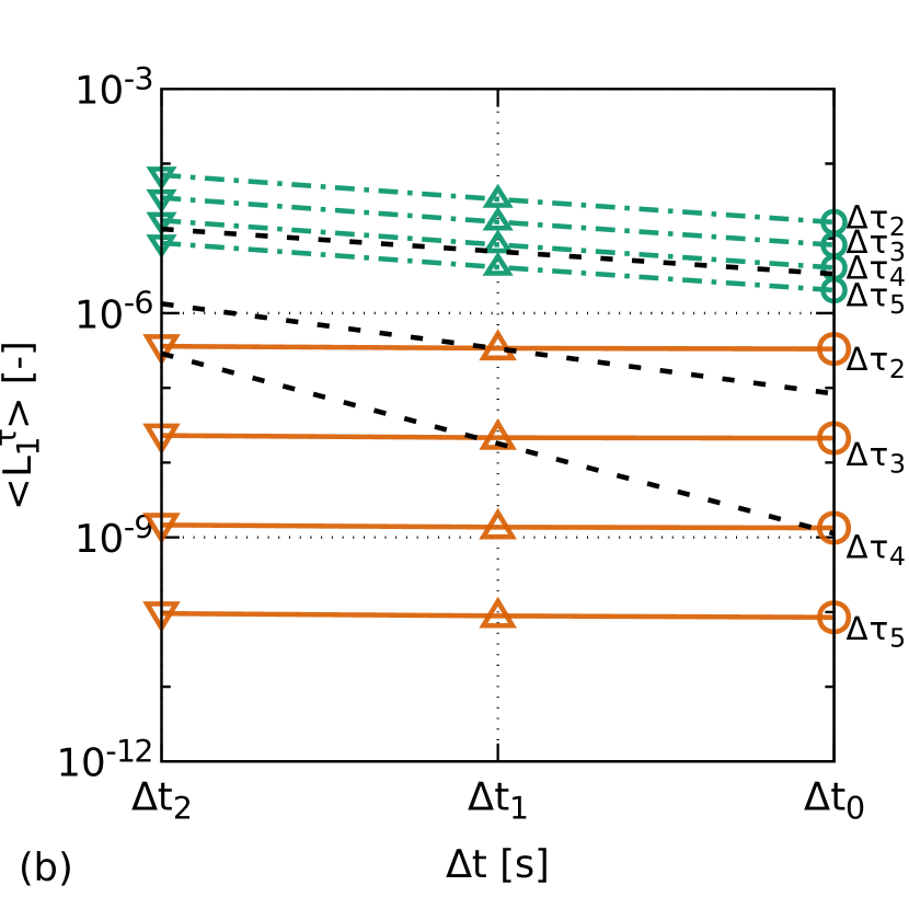
Figure 7: The convergence rate of averaged $L_{1}^{\tau}$ norms from Fig. 6, see Eq. (34). The diagrams (a),(b) present the same results and illustrate the joint convergence rate of advection and re-initialization equations (9)-(10) during revolution of circular interface using the Eulerian (green dashed-dotted lines) and Lagrangian (orange solid lines) schemes with three $C\!u_{l}$, i.e., $\Delta t_{l}$ time steps $l\!=\!0,1,2$ on four grids, i.e., the four $\Delta\tau_{k}=\sqrt{2}\Delta x_{k}/4$, $k=2,\ldots,5$ re-initialization time steps. The dashed-black lines depict slopes of the first, second and third order convergence rates, respectively.

To investigate in more details convergence rates illustrated in Fig. 6, the $L_{1}^{\tau}$ norms depicted in this figure are averaged in times $t$ and $\tau$ revealing information about the joint convergence rate of the advection and re-initialization equations (9)-(10), see Eq. (34) explaining how $\langle L_{1}^{\tau}\rangle$ in Fig. 7 is calculated. The results in Fig. 7(a)(b) obtained with the Eulerian scheme (green dashed-dotted lines) show the first order convergence rate with respect to $\Delta\tau_{k}$ and $\Delta t_{l}$ whereas the results obtained with the new Lagrangian scheme (orange solid lines) reveal the third-order convergence rate with regard to $\Delta\tau_{l}$ and they remain almost constant with regard to time $\Delta t_{l}$. In fact $\langle L_{1}^{\tau}\rangle$ decreases slightly for different $\Delta t_{l}$, $l\!=\!0,1,2$ as it can be deduced from the right column in Fig. 6. Fig. 7(b) shows that re-initialization dominates the convergence rate of Eqs. (9) and (10) in the time domain when the Lagrangian scheme is used. Hence, when CIS and the new Lagrangian scheme are used together to solve Eqs. (9) and (10), the convergence rate of advection and re-initialization is the same as the theoretical order of accuracy of the TVD Runge-Kutta scheme used to integrate Eq. (10) in time $\tau$, this result is related to the definition of $\Delta\tau_{k}\!=\!\epsilon_{h}\!=\!\sqrt{2}\Delta x_{k}/4$, $k\!=\!2,\ldots,5$. From this comparison it may be deduced the Lagrangian scheme does not introduce additional disturbances to the shape of the transported interface as its the case with its Eulerian counterpart. Hence, re-initialization governs temporal and spatial convergence when Eq. (9) is dicretized using Eqs. (23) and Eqs. (28)-(29).

In Fig. 8, the convergence rates of mass or volume of the advected circular interface are presented for three $C\!u_{l}$ numbers $l\!=\!0,1,2$ (top to bottom) on four gradually refined grids $m_{k}$, $k\!=\!2,\ldots,5$.

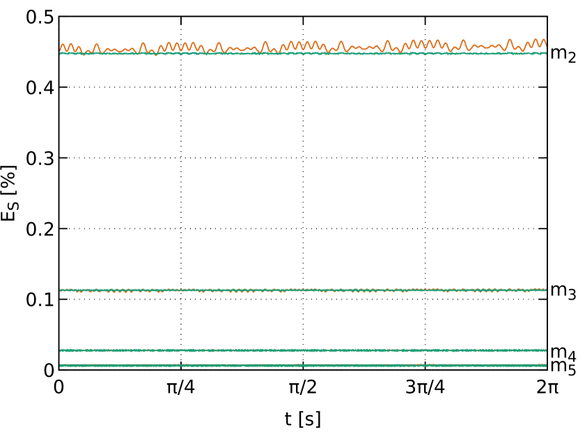
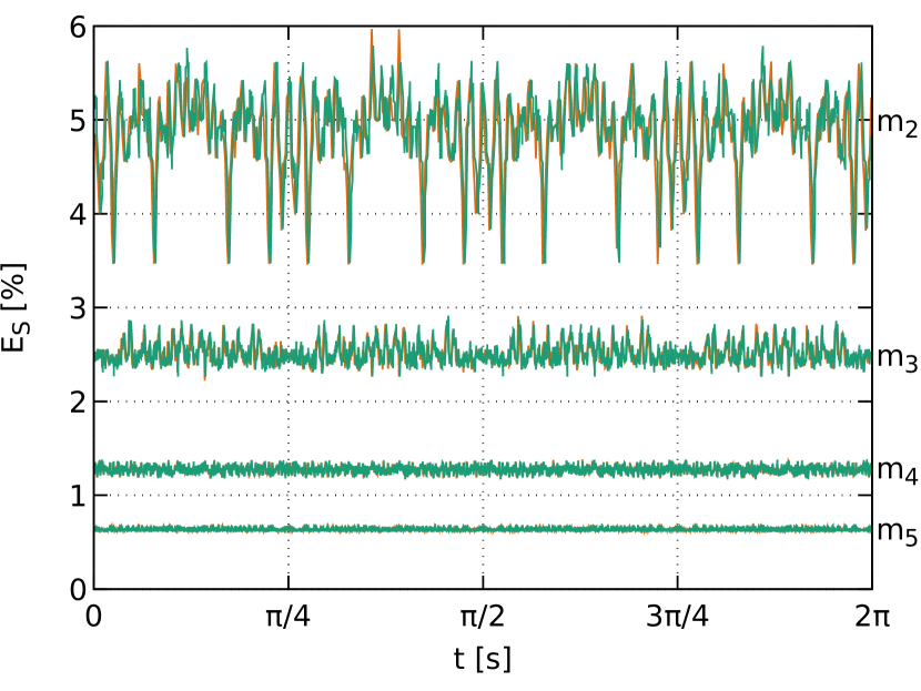
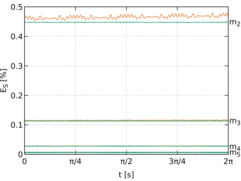
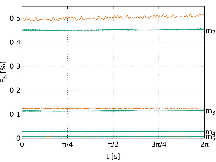
Figure 8: The convergence of mass in regions $R_{1}\!=\!\left\{x_{i}|\alpha\left(\psi\right)\geq 0.5\right\}$ (left) and $R_{2}\!=\!\left\{x_{i}|\psi\left(\alpha\right)\leq 8\epsilon_{h}\right\}$ (right) during advection of the solid body with the Eulerian (green solid line) and Lagrangian (orange solid line) schemes on four gradually refined grids $m_{k},\,k=2,\ldots,5$ and three different CFL numbers $C\!u_{0}\approx 0.35$, $C\!u_{1}\approx 0.7$, $C\!u_{2}\approx 1.4$ (from top to bottom). The number of re-initialization steps $N_{\tau}=4$ per $\Delta t$, $\Delta\tau=\epsilon_{h}$.

The errors $E_{S}$ introduced to the surface determined by the advected interface are computed using Eq. (38) after each time step $\Delta t$ and at the end of each re-initialization cycle. As it was proposed by Wacławczyk [2015], convergence of the mass is investigated in the two regions: $R_{1}\!=\!\left\{x_{i}|\alpha\left(\psi\right)\geq 0.5\right\}$, $R_{2}\!=\!\left\{x_{i}|\psi\left(\alpha\right)\leq 8\epsilon_{h}\right\}$ where $x_{i}$, $i\!=\!1,\ldots,N_{c}$ denotes the center of control volume belonging to one of the grids $m_{k}$, $k\!=\!2,\ldots,5$. The definitions of $R_{1}$, $R_{2}$ regions exploit the two, equivalent representations of the interface by $\alpha\left(\psi\!=\!0\right)=1/2$ or $\psi\left(\alpha\!=\!1/2\right)\!=\!0$, respectively.

Surprisingly, convergence of mass illustrated in Fig. 8 does not exhibit strong dependence on the advection scheme or $C\!u_{l}$ number used in the simulations, compare with the re-initialization equation norms $L_{1}^{\tau}$ and $\langle L_{1}^{\tau}\rangle$ depicted in Figs. 6 – 7. The convergence histories of mass recorded during one revolution of circular interface are almost identical for the Eulerian and Lagrangian schemes. The largest differences are visible on the coarsest grids $m_{2}$ and $m_{3}$ in the region $R_{2}$, see right column in Fig. 8 for $C\!u_{2}$. The oscillations of the mass are larger in the case of Lagrangian scheme, whereas the Eulerian scheme obtains less oscillatory mass convergence errors; on the grids $m_{4},m_{5}$ the results obtained using Eulerian and Lagrangian schemes are almost identical in both regions $R_{1},\,R_{2}$ and for all $C\!u_{l}$, $l\!=\!0,1,2$. In the case of both: Eulerian and Lagrangian schemes, the mass convergence is achieved independent from $C\!u_{l}$, $l\!=\!0,1,2$ used in the simulation.

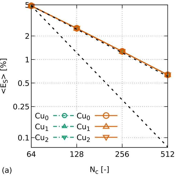
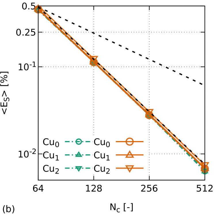
Figure 9: The averaged in time $t$ errors $E_{S}$ from Fig. 8 computed using Eq. (39) in regions $R_{1}\!=\!\left\{x_{i}|\alpha\left(\psi\right)\geq 0.5\right\}$ (a) and $R_{2}\!=\!\left\{x_{i}|\psi\left(\alpha\right)<8\epsilon_{h}\right\}$ (b). The results are obtained using the Eulerian (green dashed-dotted lines) and Lagrangian (orange solid lines) advection schemes for the three $C\!u_{l}$, $l\!=\!0,1,2$ numbers. The black dashed-lines represent, respectively, the first and second order convergence slopes.

The order of the convergence rate of mass depends on the interface representation by $\alpha\left(\psi\!=\!0\right)\!=\!1/2$ or $\psi\left(\alpha\!=\!1/2\right)\!=\!0$ as it is discussed by Wacławczyk [2015]. Based on the results in Fig. 8 it can be deduced that in the region $R_{1}$ the first-order mass convergence rate is achieved, whereas in $R_{2}$ the second order mass convergence rate is achieved for all $C\!u_{l}$, $l\!=\!0,1,2$. This is confirmed by the averaged in time $t$ errors $E_{S}$ from Fig. 8 illustrated in Fig. 9; the averaged errors $\langle E_{S}\rangle$ are computed using Eq. (39).

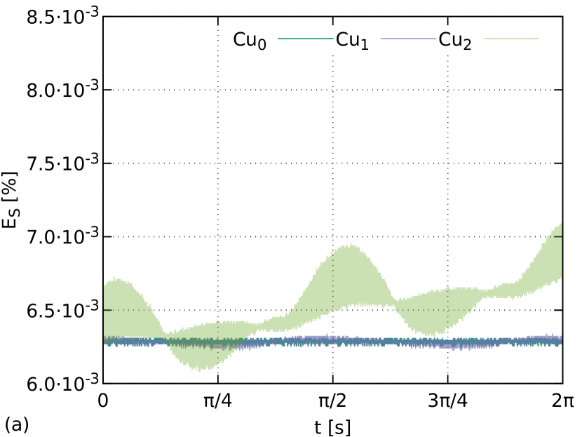
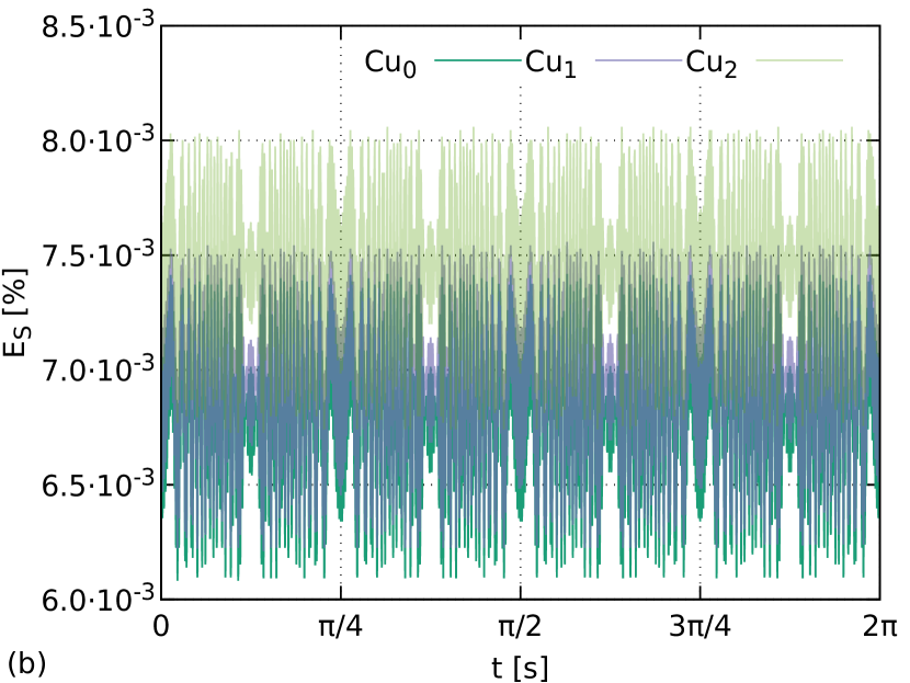
Figure 10: The convergence of mass in the region $R_{2}\!=\!\left\{x_{i}|\psi\left(\alpha\right)<8\epsilon_{h}\right\}$ on the grid $m_{5}$ during advection of the solid body with Eulerian (a) and Lagrangian (b) schemes on the grid $m_{5}$ with $C\!u_{0}\approx 0.35$, $C\!u_{1}\approx 0.7$, $C\!u_{2}\approx 1.4$. The number of re-initialization steps $N_{\tau}\!=\!4$ per time step $\Delta t$, $\Delta\tau\!=\!\epsilon_{h}$, these results are also depicted in Fig. 8.

The closer inspection of the mass convergence results on the finest grid $m_{5}$ in region $R_{2}$ is illustrated in Fig. 10. This comparison demonstrates the mass errors obtained using the Eulerian scheme are more sensitive to the selected time step size $\Delta t_{l}$, $l\!=\!0,1,2$. The results presented in Fig. 10 indicate that for $C\!u_{0}\approx 0.35$, $C\!u_{1}\approx 0.7$ Eulerian scheme can achieve better mass conservation (the error level and its oscillations are lower) than the Lagrangian scheme. When $C\!u_{2}\approx 1.4$, slow but constant divergence of the mass occurs in the case of advection carried out with the Eulerian scheme. In contrast, the errors in mass conservation achieved with the Lagrangian scheme seem to be almost unaffected by the increment in the time step size $\Delta t_{l}$, see Fig. 10(b). The errors obtained with the Lagrangian scheme indicate no change in the mass or volume of the advected circular shape during the whole revolution for all tested Currant numbers. Hence, in the case of Lagrangian scheme the mass is conserved during one revolution of the circular interface when the conditions used to derive Eqs. (28) and (29) are satisfied.

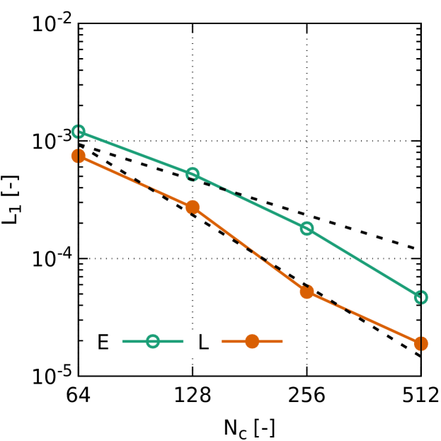
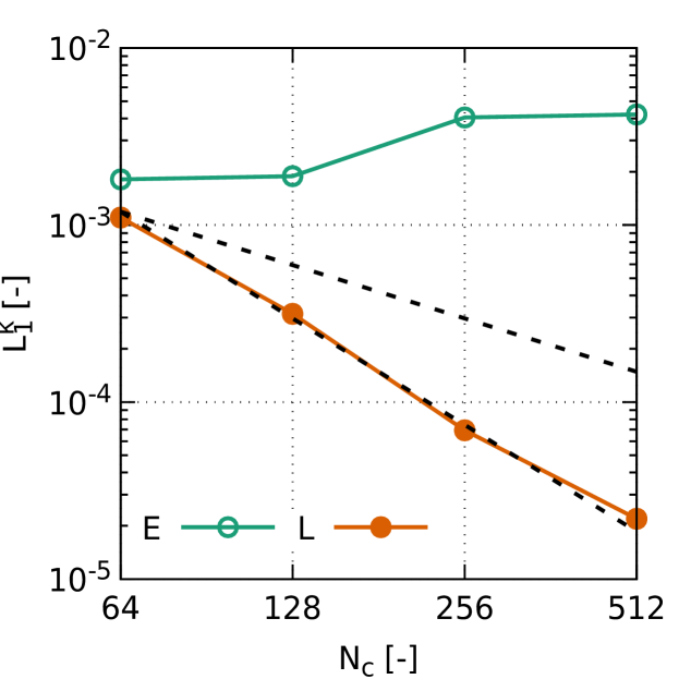
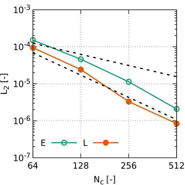
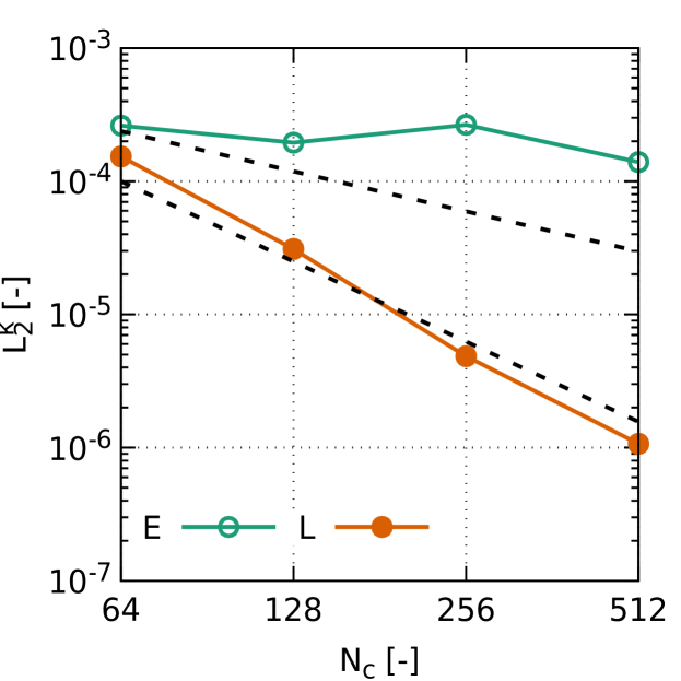
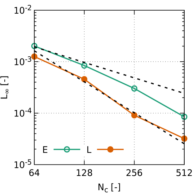
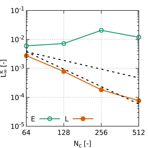
Figure 11: The convergence of $L_{1},\,L_{2},\,L_{\infty}$ norms defined by Eqs. 35–37 for $C\!u_{0}\approx 0.35$ computed after one revolution of the circular interface. The convergence of the interface shape (left), the convergence of the interface curvature (right). Symbols $E,\,L$ denote results obtained with the Eulerian or Lagrangian schemes, the black dashed lines depict the first and second order convergence slopes.

Figs. 11 – 13 illustrate the convergence rates of the interface shape and curvature on gradually refined grids $m_{k}$, $k\!=\!2,\ldots,5$. The interface shape and curvature are defined, respectively, by the level-sets of the signed-distance function $\psi\left(\alpha\!=\!1/2\right)\!=\!0$ and corresponding curvature $\kappa\left[\psi\left(\alpha\!=\!1/2\right)\!=\!0\right]\!=\!1/R$. The convergence rates illustrated in Figs. 11 – 13, for three $C\!u_{l}$, $l\!=\!0,1,2$ numbers are computed at the end of one revolution of the circular interface. In the left column the convergence rates of the interface shape, in the right column the convergence rates of the interface curvature (denoted using superscript $\kappa$) are presented. The norms $L_{1}$, $L_{2}$, $L_{\infty}$ in Figs. 11 – 13 are defined by Eqs. (35)-(37) in a similar manner for level-sets of the interface shape and curvature, information how they are computed can be found in A.

Fig. 11 reveals that only the Lagrangian scheme achieves the second-order convergence rate of both: the interface shape and curvature, compare the diagrams in left and right columns. This convergence is however affected by the selected time steps size $\Delta t_{l}$, $l\!=\!0,1,2$. The larger the Courant number is, the less obvious the order of the convergence rate, although, the second-order trend can still be deduced from the results presented in Figs. 12 – 13.

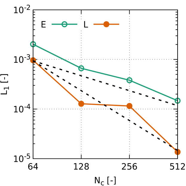
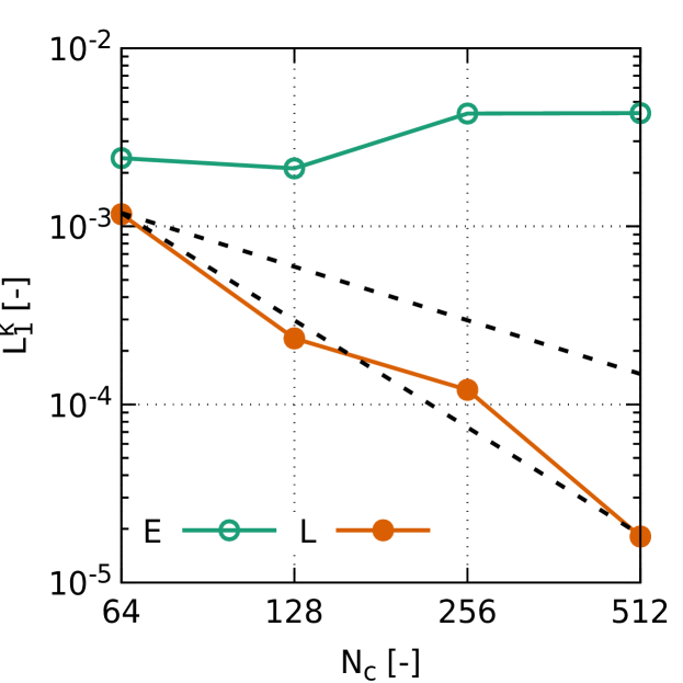
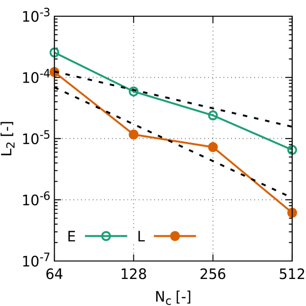
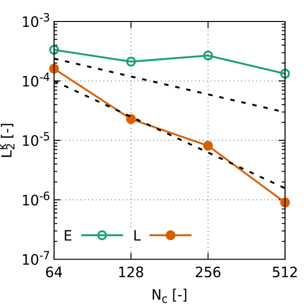
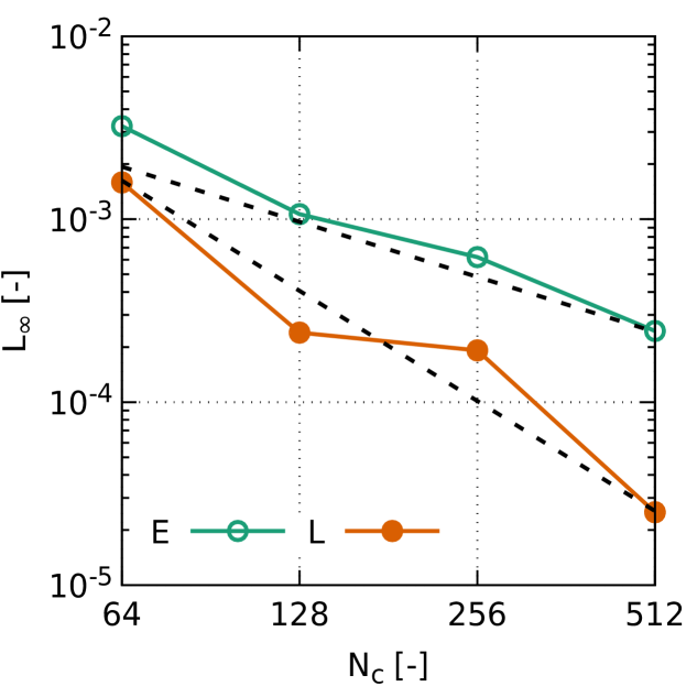
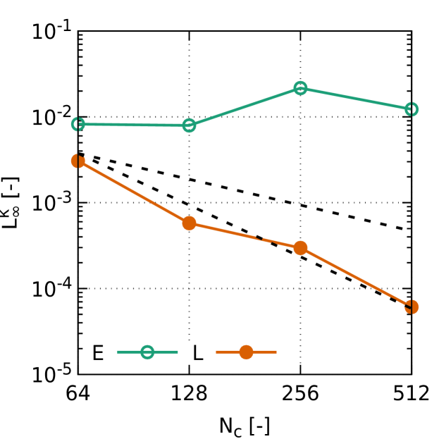
Figure 12: The convergence of $L_{1},\,L_{2},\,L_{\infty}$ norms defined by Eqs. 35–37 for $C\!u_{1}\approx 0.7$ computed after one revolution of the circular interface. The convergence of the interface shape (left), the convergence of the interface curvature (right). Symbols $E,\,L$ denote results obtained with the Eulerian or Lagrangian schemes, the black dashed lines depict the first and second order convergence slopes.

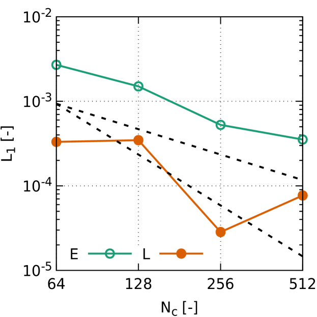
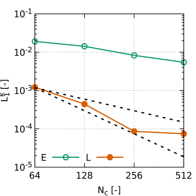
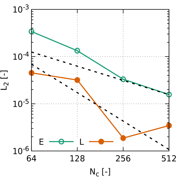
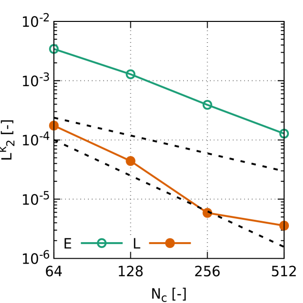
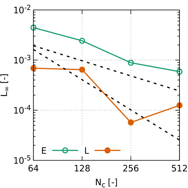
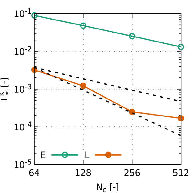
Figure 13: The convergence of $L_{1},\,L_{2},\,L_{\infty}$ norms defined by Eqs. 35–37 for $C\!u_{2}\approx 1.4$ computed after one revolution of the circular interface. The convergence of the interface shape (left), the convergence of the interface curvature (right). Symbols $E,\,L$ denote results obtained with the Eulerian or Lagrangian schemes, the black dashed lines depict the first and second order convergence slopes.

In the case of the results obtained with $C\!u_{0}\approx 0.35$ in Fig. 11 there is no doubt that the complete second-order convergence rate is achieved with the Lagrangian scheme. The growing uncertainty in the convergence rate of the interface shape and curvature observed in Figs. 12 – 13 may be related to the explicit formulation of the Lagrangian scheme proposed in the present paper.

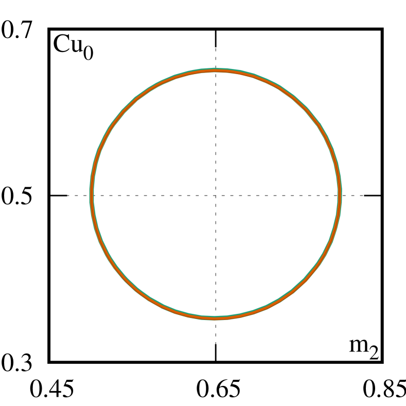
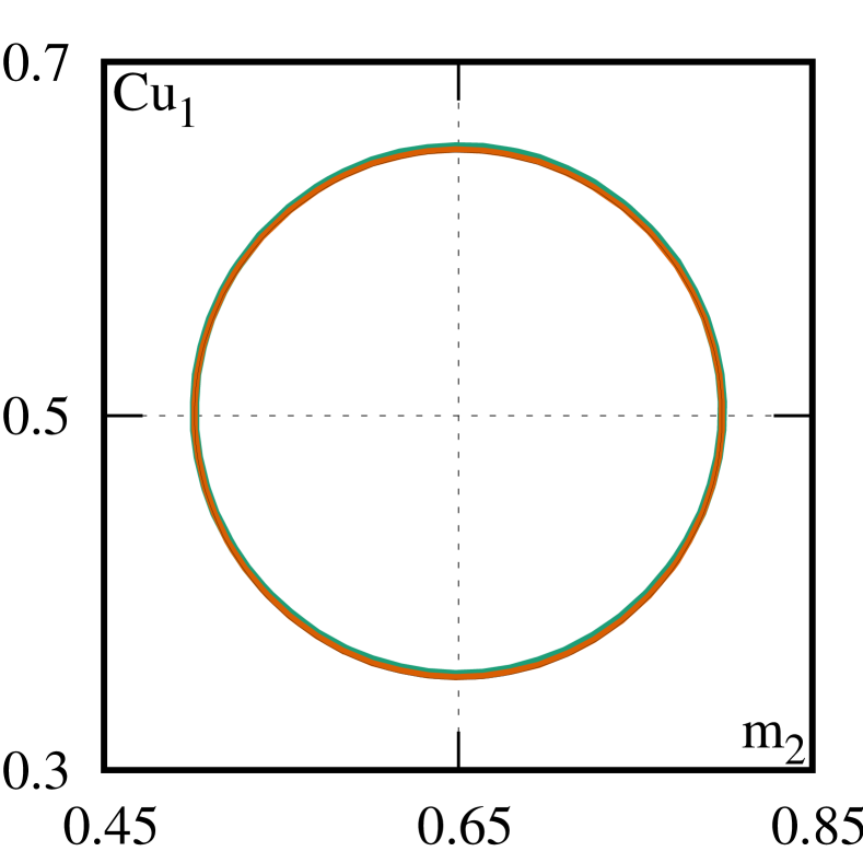
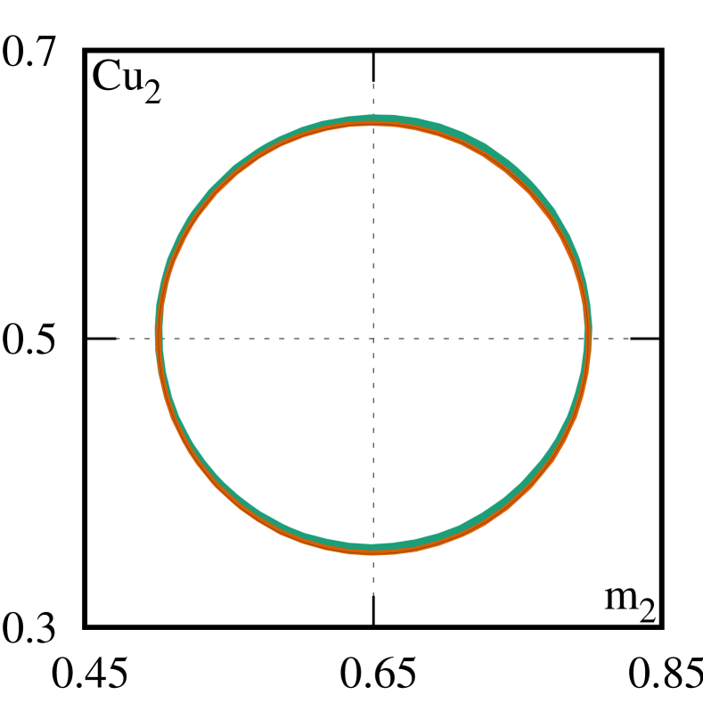
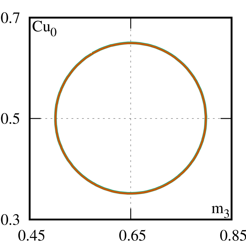
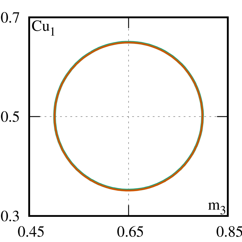
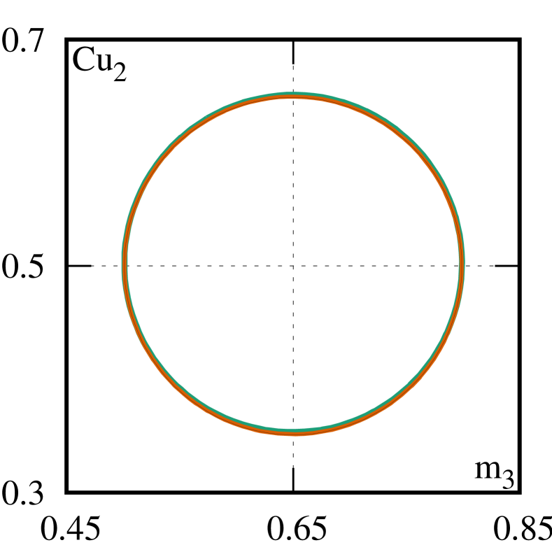
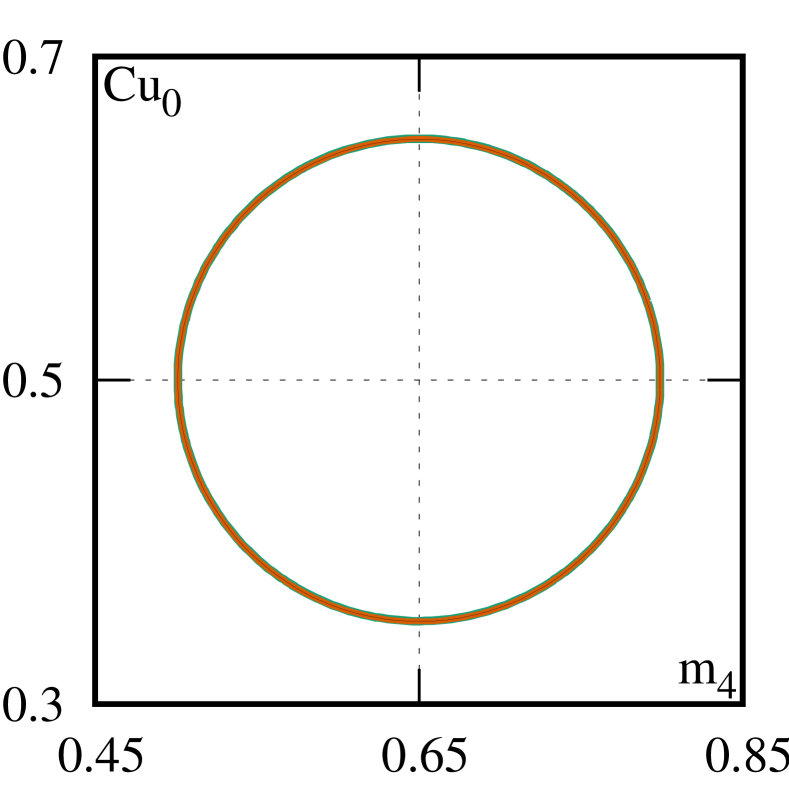
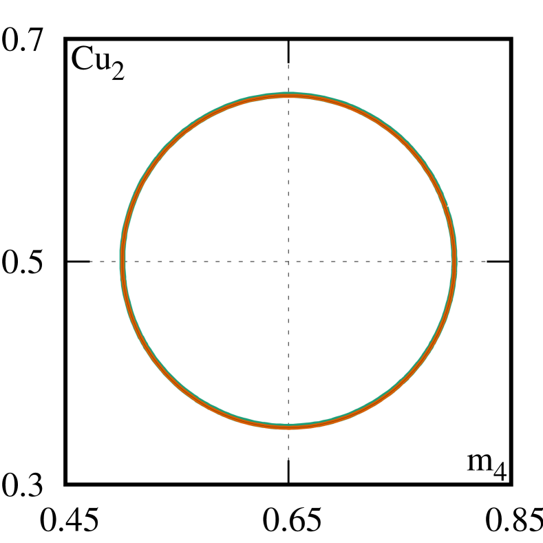
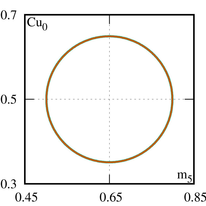
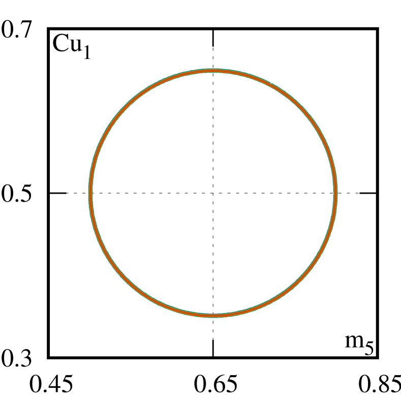
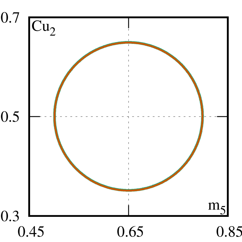
Figure 14: The level-sets $\psi\left(\alpha\!=\!1/2\right)\!=\!0$ of the circular interface shape after one revolution with $C\!u_{l}$, $l\!=\!0,1,2$ (left to right) on four grids $m_{k}\!=\!2^{4+k}\times 2^{4+k}$, $k=2,\ldots,5$ (top to bottom). The results are obtained with the Lagrangian (orange solid line) and Eulerian (green solid line) advection schemes, the exact position of the interface is depicted with the black solid line.

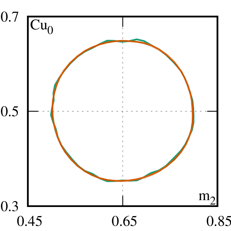
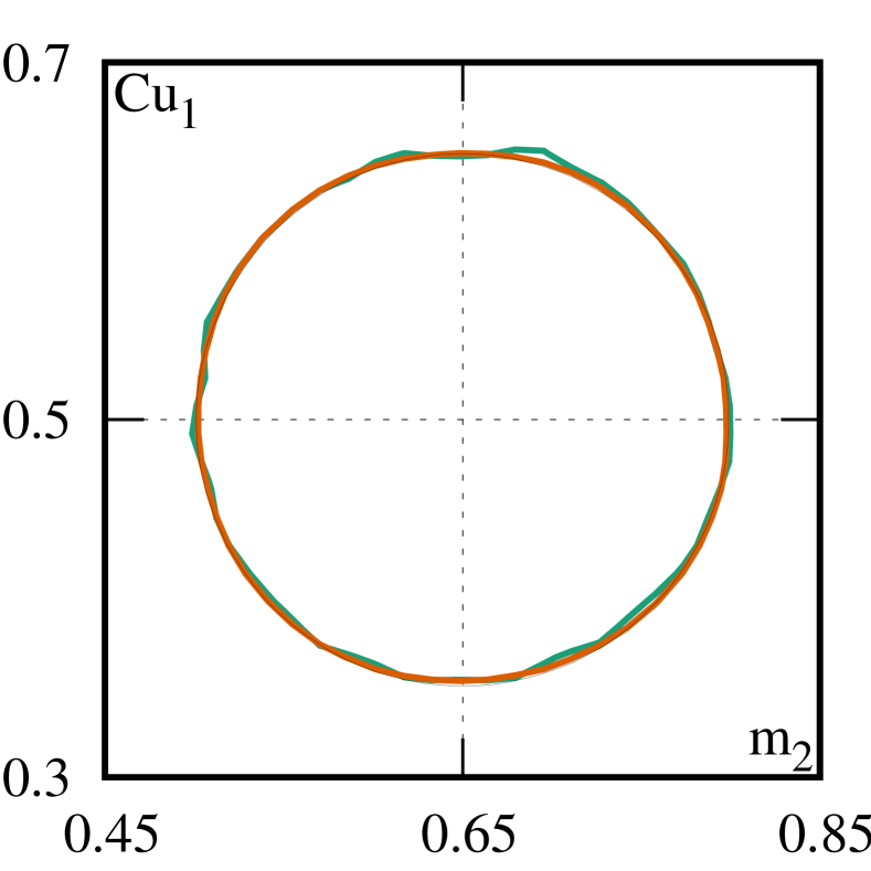
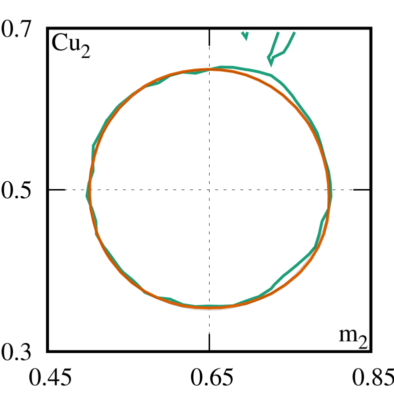
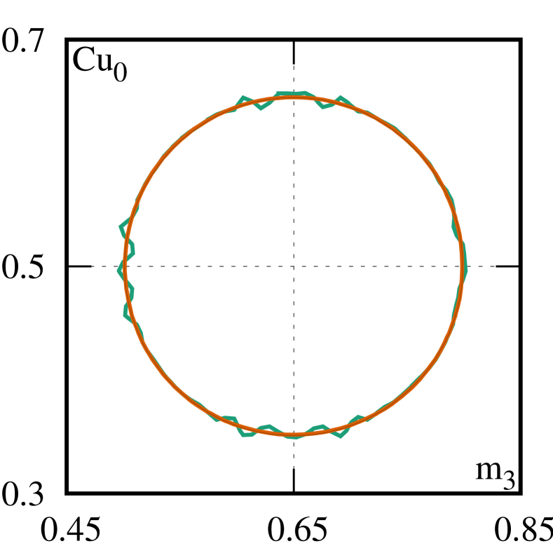
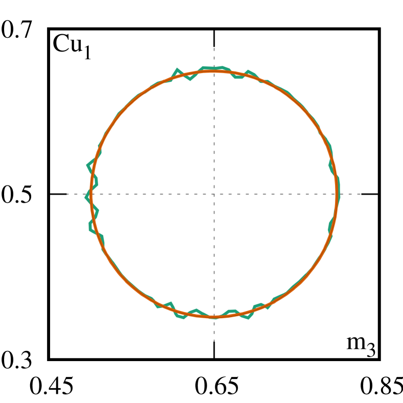
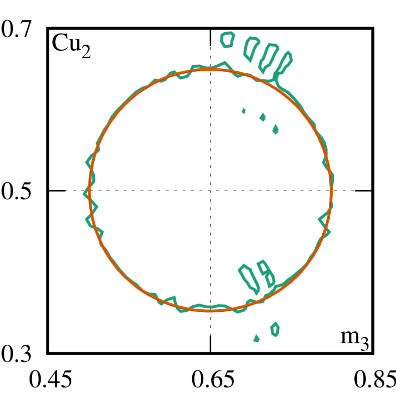
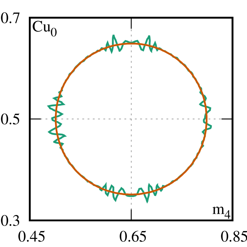
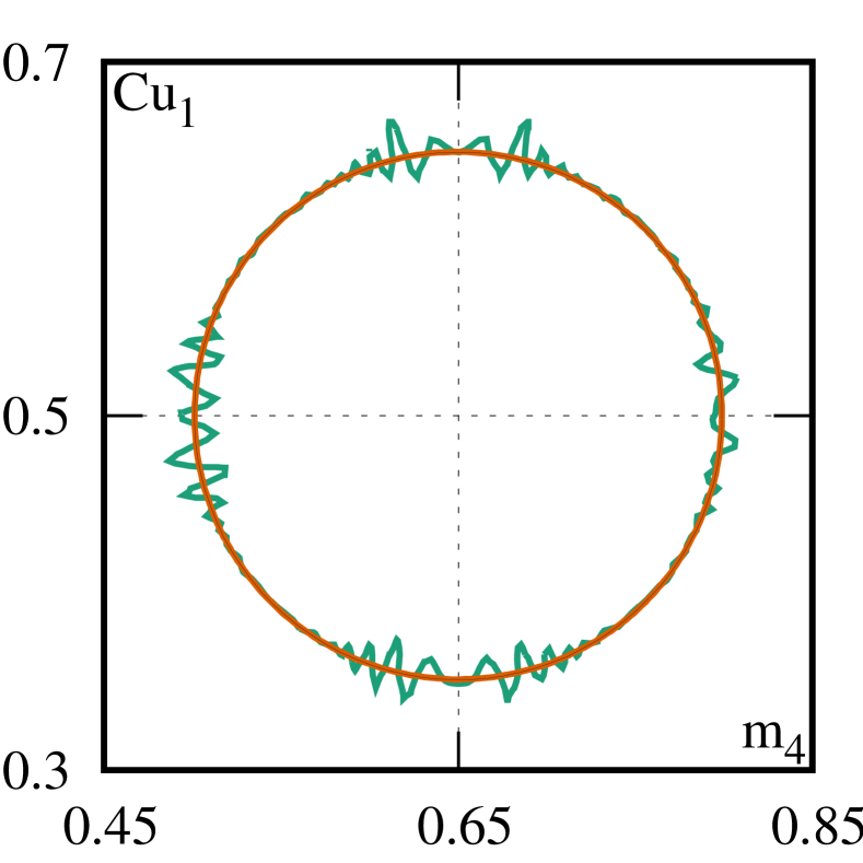
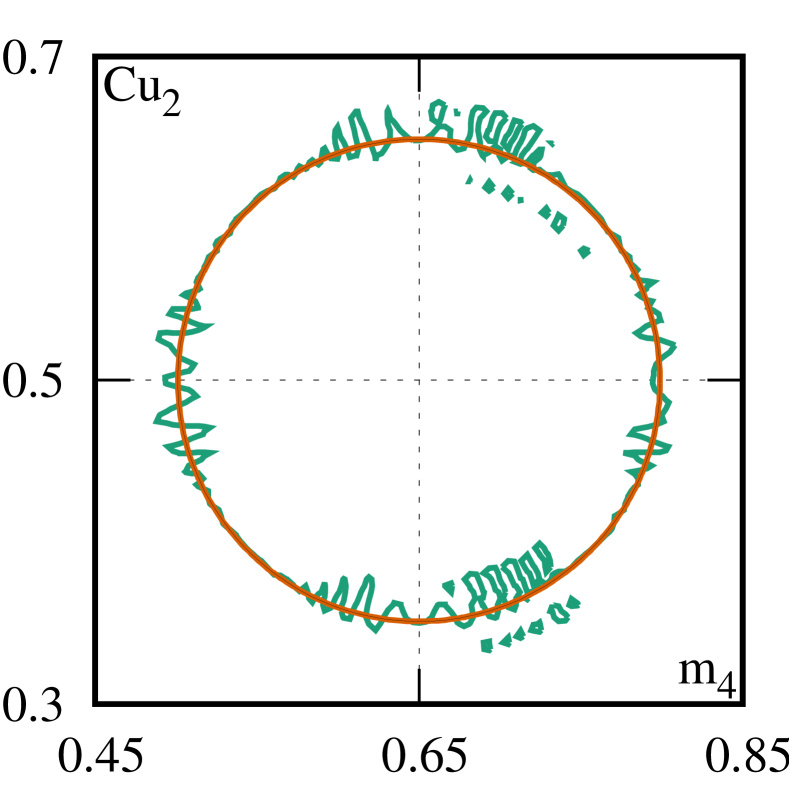
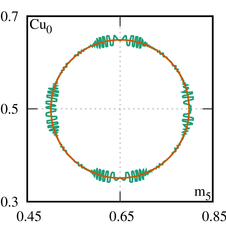
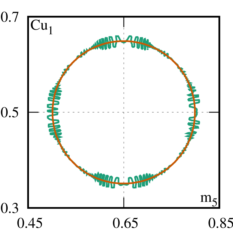
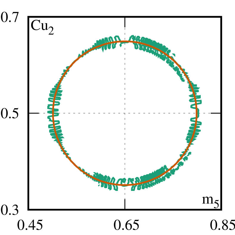
Figure 15: The level-sets of curvature $\kappa\left[\psi\left(\alpha\!=\!1/2\right)\!=\!0\right]\!=\!1/R$ of the circular interfaces from Fig. 14 after one revolution with $C\!u_{l}$, $l\!=\!0,1,2$ (left to right) on four grids $m_{k}\!=\!2^{4+k}\!\times\!2^{4+k}$, $k\!=\!2,\ldots,5$ (top to bottom). The results are obtained with the Lagrangian (orange solid line) and Eulerian (green solid line) advection schemes, the exact position of the interface curvature $\kappa=1/R$ is depicted with the black solid line.

Results in Figs. 11 – 13 show the implicit Eulerian scheme allows for second-order convergence rate of the interface shape when $C\!u_{0}\approx 0.35$. Interestingly, the interface shape convergence rates of the implicit Eulerian scheme, does not show oscillatory character unlike the solution obtained with the explicit Lagrangian scheme, even for $C\!u_{2}\approx 1.4$, see Fig. 13. In Figs. 11 – 13, it is observed that for the Eulerian scheme the order of convergence rate of the interface becomes lower, changing from second for $C\!u_{0}$ towards the first order for $C\!u_{1},\,C\!u_{2}$. This results does not correspond with the mass convergence presented in Fig. 9(b) where second order convergence was predicted for all $C\!u_{l}$, $l\!=\!0,1,2$. The reason of this discrepancy is related to integration and averaging used to compute, respectively, $E_{S}$ and $\langle E_{S}\rangle$ in Figs. 8 – 9 whereas Figs. 11 – 13 present the instantaneous errors.

The results in the right column in Figs. 11 – 13 demonstrate the interface curvature does not converge with the gradual mesh refinement when the Eulerian scheme is used. In Figs. 14 – 15 this result may be investigated in detail. Fig. 14 illustrates shapes of the circular interface defined by the level-set $\psi\left(\alpha\!=\!1/2\right)\!=\!0$ after one revolution on four grids $m_{k}$, $k=2,\ldots,5$ and for the three $C\!u_{l}$, $l\!=\!0,1,2$ numbers, obtained with the Eulerian (green solid lines) and Lagrangian (orange solid line) schemes. The reconstructed shapes of the circular interface are compared with the exact analytic solution (black solid line) confirming convergence towards the analytic solution of both the Eulerian and Lagrangian schemes for all $C\!u_{l}$, $l\!=\!0,1,2$. This is in agreement with the results presented in the left columns of Figs. 11 – 13.

In Fig. 15, the level-sets of exact curvature (black solid line) and reconstructed curvatures $\kappa\left[\psi\left(\alpha\!=\!1/2\right)\!=\!0\right]\!=\!1/R$ computed for the corresponding circular interfaces from Fig. 14 are compared. These results explain the apparent convergence of curvature observed for the Eulerian scheme and the Courant number $C\!u_{2}$, see Fig. 13(right). The corresponding level-sets of curvatures (green solid line) illustrate lack of convergence when the Eulerian scheme is used. All level-sets of curvature obtained with the Eulerian scheme show nonphysical oscillations, which do not vanish with the mesh refinement. The results in Fig. 15 indicate the frequency of these oscillations is amplified when $\Delta x_{k}\to 0$. The origin of these errors is unclear, it is supposed they are artifacts introduced by the second order flux limiter controlling only the slope of $\alpha\left(\psi\right)$.

In the case of the new Lagrangian scheme the agreement between the exact (black solid line) and reconstructed (orange solid line) curvatures is excellent. On the finest grid $m_{5}$ it is hard to find any differences between the analytic contour and its numerical approximation for all $C\!u_{l}$, $l\!=\!0,1,2$ used in the present study. We recall here, these results are obtained with the second-order accurate finite volume method resulting in the second-order accurate spatial discretization of Eqs. (9) and (10).

In Figs. 11 – 13 and Figs. 14 – 15 it can be observed that in spite of the first/second-order accurate convergence rate of the interface shape with the Eulerian scheme, the level-set of curvature of the same interfaces do not show convergence towards the exact solution. Hence, numerical convergence of the interface shape is not a sufficient condition for convergence of the interface curvature. We conclude, second-order accurate TVD MUSCL used in the present work is not able to reconstruct the shape of the circular interface and its curvature during advection in the divergence free velocity field. The complete second-order convergence rate is obtained only with the Lagrangian scheme. The accuracy of reconstruction of the interface curvature during advection does not affect substantially the conservation of mass in the conservative level-set method, see Figs. 8 – 10.

Finally, let discuss validity of the assumption made after derivation of Eq. (22) about the existence of $F_{k}\!\left[\alpha\right]$ functional minimum. Based on the convergence studies of Eq. (10) presented in Fig. 2 and Figs. 6-15 we argue Eq. (22) provides the condition for existence of the functional $F_{k}\!\left[\alpha\right]$ minimum; $F_{k}\!\left[\alpha\right]$ defined by Eq. (17) is minimized by $\alpha\left(\psi\right)$ given by Eq. (6) and hence $|\nabla\psi\left(\alpha\right)|\!=\!1$.

4 Conclusions

In this paper the relation between the volume of fluid, level-set and phase-field interface models has been introduced. As a consequence, the statistical model of the non-flat interface in the state of phase equilibrium is postulated. The statistical view on the interfaces agitated by the stochastic velocity fields has been already developed in other works (e.g. Hong and Walker [2000], Brocchini and Peregrine [2001a, b], Freeze et al. [2003], Smolentsev and Miraghaie [2005], Wacławczyk and Oberlack [2011], Wacławczyk and Wacławczyk [2015]), the statistical model introduced herein is based on the ensemble averaged picture of the sharp interface disturbed by the stochastic velocity field. It is derived by the ensemble averaging of the phase indicator function transport equation (1) and the conservative closure of the correlation between the sharp interface velocity fluctuation $\mathbf{W}^{\prime}\!\cdot\!\mathbf{n}_{\Gamma}$ and the exact Dirac’s delta function $\delta\left(\Psi\right)$ indicating its instantaneous position, see Eq. (13) and Eq. (10).

Subsequently, the relation of this new model with the modified Allen-Cahn equation (4) is established showing the statistical model of the interface describes the non-flat interface in the state of phase equilibrium. This result introduces the physical interpretation of the re-initialization equation (10), determination of its stationary solution is equivalent to finding the minimum of the modified Ginzburg-Landau functional given by Eq. (17). The new term in Eq. (17) can be interpreted as the contribution to the interfacial energy density in result of a local change of the regularized interface shape and/or size. The functional derivative of this new term given by Eq. (16), resembles the model of capillary forces used in the one-fluid sharp interface formulation.

The relation between the statistical interface model and modified Allen-Cahn equation shows the CLS method is equivalent of the phase field interface model. The order parameter $\alpha\left(\psi\right)$ of this new phase field interface model is a conserved quantity, it may be interpreted as the probability of finding one of the two phases sharing the regularized interface. The probability $\alpha\left(\psi\right)$ is defined in terms of the logistic distribution where $\epsilon_{h}\!>\!0$ is measure of deviation of the instantaneous sharp interface position from its expected position, see Eqs. (6)-(7) and Eq. (12). This latter result along with the results presented by the author (see Wacławczyk [2015]) introduces the relation between the sharp and diffusive interface models, see Eqs. (9) and (10) in the limit $\epsilon_{h}\!\to\!0$.

In the second part of the present paper, two numerical techniques are introduced to reduce numerical errors during solution of Eqs. (9) and (10) and guarantee the balance of interfacial energies predicted by Eq. (22). At first, dependence of the known $\alpha\left(\psi\right)$ profile on the signed-distance function $\psi\left(\alpha\right)$ is exploited to approximate the RHS fluxes in Eq. (10) leading to the constrained interpolation scheme (CIS), see Eqs. (24). It is demonstrated, CIS improves stability of the numerical solution of Eq. (10) with regard to the selected time step size $\Delta\tau$ and avoids oscillatory errors, see Fig. 2 and Figs. 3 – 5, respectively. Furthermore, result in Figs. 6 – 7 show CIS guarantees the theoretical convergence rate of the numerical solution of Eqs. (9) and (10) on gradually refined grids during advection of the regularized interface.

Next, the new semi-analytical Lagrangian scheme for advection of $\alpha\left(\psi\right)$ and $\psi\left(\alpha\right)$ functions has been derived, see Eqs. (28) and (29). In Sec. 3.2 it is demonstrated the new advection scheme avoids introduction of the high-frequency oscillatory errors in curvature of the regularized interface, see Fig. 15. For this reason, the Lagrangian scheme reaches the theoretical second-order convergence of the interface shape and curvature, see results in Figs. 11 – 13 and Figs. 14 – 15, respectively.

Appendix A Error norms

To compute errors during the numerical solution of Eqs. (9) and (10) different error norms are used in the present work, this appendix provides their definitions. In Fig. 2, the distance between solutions on two different time $\tau$ levels is measured by the first-order norm

$$L_{1}^{\tau}=\frac{1}{N_{c}}\sum_{i=1}^{N_{c}}|\alpha_{i}^{n+1}-\alpha_{i}^{n}|,$$ (31)

where $N_{c}$ is the number of control volumes and $n+1$ denotes a new time level $\tau$, summation is performed over the control volumes centers in the entire computational domain $\Omega$. In Fig. 6, $L_{1}^{\tau}$ norm is plotted after each time step $\Delta t$.

In Figs. 3-5, normalized first-order norms are used to visualize numerical errors introduced by LIS or CIS interpolation during re-initialization

$$L_{1,an}\left(\phi\right)=\frac{|\phi_{an}-\phi_{num}|}{|\phi_{an}|+\epsilon},$$ (32)

$$L_{1,max}\left(\phi\right)=\frac{|\phi_{an}-\phi_{num}|}{\phi_{an,max}},$$ (33)

where values $\phi_{an}$, $\phi_{num}$ are calculated, respectively, analytically and numerically in each control volume, $\epsilon\!=\!5\cdot 10^{-16}$ and $\phi\!=\!\alpha$, or is the first component of $\nabla\alpha$ or $\nabla^{2}\alpha$. $L_{1,max}\left(\phi\right)$ norm is obtained using $\phi_{an,max}\!=\!max\left[\phi_{an,i}\right]$ where $i\!=\!1,\ldots,N_{c}$.

In Fig. 7 the averaged in times $t$ and $\tau$ norms $L_{1}^{\tau}$ given by Eq. (31) are summarized, the averaged norms are calculated according to the formula

$$\langle L_{1}^{\tau}\rangle=\frac{1}{N_{\tau}N_{t}}\sum_{m=1}^{N_{t}}\sum_{n=1}^{N_{\tau}}L_{1,m,n}^{\tau},$$ (34)

where $N_{t},\,N_{\tau}$ denote the number of time steps $\Delta t,\,\Delta\tau$, respectively.

In Figs. 11 – 13 $L_{1}$, $L_{2}$ and $L_{\infty}$ norms are used to investigate convergence of the interface shape and curvature, their definitions read

$$L_{1}=\frac{1}{N_{p}}\sum_{l=1}^{N_{p}}|\phi_{e}^{l}-\phi_{n}^{l}|,$$ (35)

$$L_{2}=\frac{1}{N_{p}}\left[\sum_{l=1}^{N_{p}}\left(\phi_{e}^{l}-\phi_{n}^{l}\right)^{2}\right]^{1/2},$$ (36)

$$L_{\infty}=max\left[|\phi_{e}^{l}-\phi_{n}^{l}|\right],\,\,\text{where}\,\,l\!=\!1,\ldots,N_{p}$$ (37)

and $N_{p}$ denotes the number of probes on the contour $\phi$ representing the level-sets of the interface $\psi\left(\alpha\!=\!1/2\right)\!=\!0$ or curvature $\kappa\left[\psi\left(\alpha\!=\!1/2\right)\!=\!0\right]\!=\!1/R$ computed on the $k\!-\!th$ grid $m_{k}$ (for brevity, the grid index is omitted in Eqs. (35)-(37)), $\phi_{e}$ denotes the point on the exact level-set and $\phi_{n}$ denotes its numerical approximation. Moreover, we assume that norms $L_{1}^{\kappa}$, $L_{2}^{\kappa}$ and $L_{\infty}^{\kappa}$ computed using Eqs. (35)-(37) when $\phi$ is the level-set of $\kappa$ are dimensionless as they are divided by $\kappa_{1}=1\,[1/m]$.

Another class of the numerical error indicator is obtained by calculation of the difference between analytical and reconstructed surface/volume of the advected circular interface in Sec. 3.2. In order to measure departure of the numerical solution $S_{n}$ from the exact value $S_{e}=\pi R^{2}$ following formula is used to compute

$$E_{S}=100\cdot|1-S_{n}/S_{e}|$$ (38)

after each time step $\Delta t$ and at the end of the re-initialization cycle, i.e., after $N_{\tau}\!=\!4$ time steps $\Delta\tau$. This error is averaged in time $t$ to closely inspect convergence of mass during one revolution of the circular interface, see Fig. 9; the averaging is carried out using the equation

$$\langle E_{S}\rangle=\frac{1}{N_{t}}\sum_{l=1}^{N_{t}}E_{S}^{l}.$$ (39)

Appendix B Discretization of the re-initialization equation

In this appendix, discretization of Eq. (10) in the framework of the second-order accurate finite volume method is presented. After integration of Eq. (10) in the control volume $V_{P}$, employment of the Gauss theorem and mid-point rule in centers of the faces $f$ and in center of the given control volume $P$, one obtains

$$\frac{\partial\alpha}{\partial\tau}\Bigr{|}_{P}=\frac{1}{V_{P}}\sum_{f=1}^{n_{b}}\left[\tilde{\delta}\left(\alpha\right)\left(|\nabla\psi|-1\right)\mathbf{n}_{\Gamma}\cdot\mathbf{n}\right]_{f}S_{f},$$ (40)

where $n_{b}$ is the number of neighbors of the control volume $P$, $\left[\mathbf{n}_{\Gamma}\cdot\mathbf{n}\right]_{f}$ is dot product of the normal $\mathbf{n}_{\Gamma}\!=\!\nabla\psi/|\nabla\psi|$ interpolated at the face $f$ and normal $\mathbf{n}_{f}\!=\!\mathbf{S}_{f}/|\mathbf{S}_{f}|$ where $\mathbf{S}_{f}$ denotes surface vector of the face $f$; $\tilde{\delta}\left(\alpha_{f}\right)\!=\!\alpha_{f}\left(1-\alpha_{f}\right)$ is approximated using the linear interpolation (LIS) on the face $f\!=\!e$ leading to $\alpha_{e}\!=\!\left(\alpha_{P}\!+\!\alpha_{E}\right)/2$, or constrained interpolation (CIS) defined by Eqs. (24).

$|\nabla\psi|$ in Eq. (40) is computed using the second-order central-difference approximation of $\nabla\psi$ components; at the face $f\!=\!e$ this approximation reads

$$\begin{split}\frac{\partial\psi}{\partial x_{1}}\Big{|}_{e}&\approx\frac{\left(\psi_{E}-\psi_{P}\right)}{\Delta x},\\ \frac{\partial\psi}{\partial x_{2}}\Big{|}_{e}&\approx\frac{\left(\psi_{N}+\psi_{NE}-\psi_{S}-\psi_{SE}\right)}{4\Delta y},\\ \end{split}$$ (41)

where subscript $E,N,T,\ldots$ represent the centers of the neighbor control volumes on uniform, orthogonal structured grid.

References

- Aarts et al. [2004] Aarts, D. G. A. L., Schmidt, M., Lekkerkerker, H. N. W., 2004. Direct visual observation of thermal capillary waves. Science, 304, 847–850. doi:10.1126/science.1097116.
- Allen and Cahn [1979] Allen, S., Cahn, J., 1979. A microscopic theory for antiphase domain boundary motion and its application to antiphase domain coarsening. Acta Metall., 27, 1085–1095.
- Anderson et al. [1998] Anderson, D. M., McFadden, G. B., Wheeler, A. A., 1998. Diffuse-Interface Methods in Fluid Mechanics. Annu. Rev. Fluid Mech., 30, 139–165. doi:10.1146/annurev.fluid.30.1.139.
- Balakrishnan [1992] Balakrishnan, N., 1992. Handbook of the logistic distribution. Marcel Deker INC.
- Balcazar et al. [2014] Balcazar, N., Jofre, L., Lehmkuhl, O., Castro, J., Rigola, J., 2014. A finite-volume/level-set method for simulating two-phase flows on unstructured grids. Int. J. Multiphase Flow, 64, 55 – 72. doi:http://dx.doi.org/10.1016/j.ijmultiphaseflow.2014.04.008.
- Bao et al. [2012] Bao, K., Shi, Y., Sun, S., Wang, X.-P., 2012. A finite element method for the numerical solution of the coupled Cahn-Hilliard and Navier-Stokes system for moving contact line problems. J. Comp. Phys., 231, 8083 – 8099. doi:http://dx.doi.org/10.1016/j.jcp.2012.07.027.
- Brassel and Bretin [2011] Brassel, M., Bretin, E., 2011. A modified phase field approximation for mean curvature flow with conservation of the volume. Math. Method. Appl. Sci., 34, 1157–1180. URL: http://dx.doi.org/10.1002/mma.1426. doi:10.1002/mma.1426.
- Brocchini and Peregrine [2001a] Brocchini, M., Peregrine, D. H., 2001a. The dynamics of strong turbulence at free surfaces. Part 1. Description. J. Fluid Mech., 449, 225–254.
- Brocchini and Peregrine [2001b] Brocchini, M., Peregrine, D. H., 2001b. The dynamics of strong turbulence at free surfaces. Part 2. Free-surface boundary conditions. J. Fluid Mech., 449, 255–290.
- Cahn and Hilliard [1958] Cahn, J. W., Hilliard, J. E., 1958. Free Energy of a Nonuniform System. I. Interfacial Free Energy. J. Chem. Phys., 28, 258–267. doi:http://dx.doi.org/10.1063/1.1744102.
- Chiu and Lin [2011] Chiu, P.-H., Lin, Y.-T., 2011. A conservative phase field method for solving incompressible two-phase flows. J. Comp. Phys., 230, 185–204. doi:http://dx.doi.org/10.1016/j.jcp.2010.09.021.
- Fedeli [2017] Fedeli, L., 2017. Computer simulations of phase field drops on super-hydrophobic surfaces. J. Comp. Phys., 344, 247–259. doi:http://dx.doi.org/10.1016/j.jcp.2017.04.068.
- Ferziger and Perić [2002] Ferziger, J. H., Perić, M., 2002. Computational Methods for Fluid Dynamics. Springer Verlag, Berlin Heidelberg New York.
- Freeze et al. [2003] Freeze, B., Smolentsev, S., Morley, N., M., A., 2003. Characterization of the effect of Froude number on surface waves and heat transfer in inclined turbulent open channel flows. Heat Mass Transfer, 46, 3765–3775.
- Gottlieb and Shu [1998] Gottlieb, S., Shu, C.-W., 1998. Total variation diminishing Runge-Kutta schemes. Math. Comp., 67, 73–85.
- Herrmans [2005] Herrmans, M., 2005. Refined Level-Set Grids method for tracking interfaces. In Annual Research Briefs (pp. 3–18). Center of Turbulence Research, University of Stanford.
- Hong and Walker [2000] Hong, W.-L., Walker, D., 2000. Reynolds-averaged equations for free surface flows with application to high-Froude-number jet spreding. J. Fluid Mech., 417, 183–209.
- Kim et al. [2014] Kim, J., Lee, S., Choi, Y., 2014. A conservative Allen-Cahn equation with a spacetime dependent Lagrange multiplier. Int. J. Eng. Sci., 84, 11 – 17. doi:http://dx.doi.org/10.1016/j.ijengsci.2014.06.004.
- McCaslin and Desjardins [2014] McCaslin, J. O., Desjardins, O., 2014. A localized re-initialization equation for the conservative level set method. J. Comp. Phys., 262, 408 – 426. doi:http://dx.doi.org/10.1016/j.jcp.2014.01.017.
- Moelans et al. [2008] Moelans, N., Blanpain, B., Wollants, P., 2008. An introduction to phase-field modeling of microstructure evolution. Calphad, 32, 268 – 294. doi:http://dx.doi.org/10.1016/j.calphad.2007.11.003.
- Olsson and Kreiss [2005] Olsson, E., Kreiss, G., 2005. A conservative level-set method for two phase flow. J. Comp. Phys., 210, 225–246.
- Osher and Fedkiw [2003] Osher, S., Fedkiw, R., 2003. Level Set Methods and Dynamic Implicit Surfaces. Springer Verlag, INC. New-York.
- Osher and Sethian [1988] Osher, S., Sethian, J. A., 1988. Fronts propagating with curvature-dependent speed: Algorithms based on Hamilton-Jacobi formulations. J. Comp. Phys., 79, 12 – 49. doi:http://dx.doi.org/10.1016/0021-9991(88)90002-2.
- Pashos et al. [2015] Pashos, G., Kokkoris, G., Boudouvis, A., 2015. A modified phase-field method for the investigation of wetting transitions of droplets on patterned surfaces. J. Comp. Phys., 283, 258 – 270. doi:http://dx.doi.org/10.1016/j.jcp.2014.11.045.
- Pope [1998] Pope, S., 1998. The evolution of surfaces in turbulence. Int. J. Eng. Sciences, 26, 445–469.
- Schäfer [2006] Schäfer, M., 2006. Computational Engineering, Introduction to Numerical Methods. Springer-Verlag Berlin Heidelberg New York.
- Smolentsev and Miraghaie [2005] Smolentsev, S., Miraghaie, R., 2005. Study of a free surface in open-channel water flows in the regime from ”weak” to ”strong” turbulence. Int. J. Multiphase Flows, 31, 921–939.
- Smoluchowski [1908] Smoluchowski, M., 1908. Molekular-kinetische Theorie der Opaleszenz von Gasen im kritischen zustande, sowie einiger verwandter erscheinungen. Ann. Phys., 330, 205–226. doi:10.1002/andp.19083300203.
- Sussman et al. [1998] Sussman, M., Fatemi, E., Smereka, P., Osher, S., 1998. An improved level set method for incompressible two-phase flows. Comput. Fluids, 27, 663 – 680. doi:http://dx.doi.org/10.1016/S0045-7930(97)00053-4.
- Sussman et al. [1994] Sussman, M., Smereka, P., Osher, S. J., 1994. A level set approach for computing solutions to incompressible two-phase flows. J. Comp. Phys., 114, 146–159.
- Tryggvason et al. [2011] Tryggvason, G., Scardovelli, R., Zaleski, S., 2011. Direct Numerical Simulations of Gas-Liquid Multiphase Flows. Cambridge University Press.
- Vrij [1973] Vrij, A., 1973. Light scattering from liquid interfaces. Chemie Ingenieur Technik, 45, 1113–1114. doi:10.1002/cite.330451807.
- van der Waals [1979] van der Waals, J., 1979. The thermodynamic theory of capillarity under the hypothesis of a continuous variation of density. J. Statist. Phys., 20, 200–244.
- Wacławczyk and Oberlack [2011] Wacławczyk, M., Oberlack, M., 2011. Closure proposals for the tracking of turbulence-agitated gas-liquid interfaces in stratified flows. Int. J. Multiphase Flow, 37, 967–976.
- Wacławczyk and Wacławczyk [2015] Wacławczyk, M., Wacławczyk, T., 2015. A priori study for the modelling of velocity-interface correlations in the stratified air-water flows. Int. J. Heat Fluid Flow, 52, 40 – 49. doi:http://dx.doi.org/10.1016/j.ijheatfluidflow.2014.11.004.
- Wacławczyk [2015] Wacławczyk, T., 2015. A consistent solution of the re-initialization equation in the conservative level-set method. J. Comp. Phys., 299, 487 – 525. doi:http://dx.doi.org/10.1016/j.jcp.2015.06.029.
- Wacławczyk and Koronowicz [2006] Wacławczyk, T., Koronowicz, T., 2006. Modelling of the free surface flows with high-resolution schemes. Chemical and Process Engineering, 27, 783–802.
- Wacławczyk and Koronowicz [2008a] Wacławczyk, T., Koronowicz, T., 2008a. Comparison of CICSAM and HRIC high resolution schemes for interface capturing. J. Theoretical and Applied Mechanics, 46, 325–345.
- Wacławczyk and Koronowicz [2008b] Wacławczyk, T., Koronowicz, T., 2008b. Remarks on prediction of wave drag using VOF method with interface capturing approach. Archives of Civil and Mechanical Engineering, 8, 5 – 14. doi:http://dx.doi.org/10.1016/S1644-9665(12)60262-3.
- Wacławczyk et al. [2014] Wacławczyk, T., Wacławczyk, M., Kraheberger, S. V., 2014. Modeling of turbulence-interface interactions in stratified two-phase flows. Journal of Physics: Conference Series, 530.
- Yue et al. [2007] Yue, P., Zhou, C., Feng, J. J., 2007. Spontaneous shrinkage of drops and mass conservation in phase-field simulations. J. Comp. Phys., 223, 1 – 9. doi:http://dx.doi.org/10.1016/j.jcp.2006.11.020.