Oscillations in aggregation-shattering processes

Abstract

We observe never-ending oscillations in systems undergoing aggregation and collision-controlled shattering. Specifically, we investigate aggregation-shattering processes with aggregation kernels $K_{i,j}=(i/j)^{a}+(j/i)^{a}$ and shattering kernels $F_{i,j}=\lambda K_{i,j}$, where $i$ and $j$ are cluster sizes and parameter $\lambda$ quantifies the strength of shattering. When $0\leq a<1/2$, there are no oscillations and the system monotonically approaches to a steady state for all values of $\lambda$; in this region we obtain an analytical solution for the stationary cluster size distribution. Numerical solutions of the rate equations show that oscillations emerge in the $1/2<a\leq 1$ range. When $\lambda$ is sufficiently large oscillations decay and eventually disappear, while for $\lambda<\lambda_{c}(a)$ oscillations apparently persist forever. Thus never-ending oscillations can arise in closed aggregation-shattering processes without sinks and sources of particles.

Two complimentary processes, aggregation and fragmentation Flory (1953); Krapivsky et al. (2010); Leyvraz (2003), occur in numerous systems that dramatically differ in their spatial and temporal scales. Reversible polymerization in solutions Flory (1953) and merging of prions (cell proteins) Poeschel et al. (2003) are typical examples on the molecular scale. On somewhat larger scales airborne particles perform Brownian motion in atmosphere and coalesce giving rise to smog droplets Shrivastava (1982). Aggregation of users in the Internet leads to the emergence of communities and forums Krapivsky et al. (2010); Dorogovtsev and Mendes (2003) which can further merge or split. Vortexes in a fluid flow merge and decompose forming turbulent cascades Zakharov et al. (2012). On much larger scales, aggregation-fragmentation processes take place in planetary rings, like Saturn rings, where the particle size distribution is determined by a subtle balance between aggregation and fragmentation of the rings particles Brilliantov et al. (2015); Stadnichuk et al. (2015); Cuzzi et al. (2010); Brilliantov et al. (2009); Esposito (2006).

In spatially homogeneous well-mixed systems, aggregation and fragmentation processes are described by an infinite set of nonlinear ordinary differential equations (ODEs) for the concentrations of clusters of various masses. Such equations are intractable apart from a few special cases. The long-time behavior, however, is occasionally known—the processes of aggregation and fragmentation act in the opposite directions and hence the cluster size distribution often becomes stationary in the long time limit . The emergence of the stationary cluster size distribution can be mathematically interpreted as the manifestation of the fixed point of the differential equations Strogatz (1994). For a single differential equation, fixed points determine the long time behavior, while for two coupled differential equations the asymptotic behavior may be determined by a fixed point or a limit cycle. In the case of infinitely many coupled ODEs, limit cycles are feasible, yet they haven’t been observed in aggregation-fragmentation processes. More precisely, there were signs of oscillations in a few open systems usually driven by constant source of monomers and by sink of large clusters. In this paper we report oscillations in a closed system undergoing aggregation and collision-controlled fragmentation.

In the most important case of binary aggregation the collision between two clusters comprising $i$ and $j$ monomers may result in the formation of a joint aggregate of $i+j$ monomers. Symbolically, $[i]+[j]\xrightarrow{K_{i,j}}[i+j],$ where $K_{ij}$ is the merging rate (see Fig. 1). Let $n_{k}$ be the concentration of clusters that contain $k$ monomers. These quantities obey the Smoluchowski equations Krapivsky et al. (2010); Leyvraz (2003):

$$\frac{dn_{k}}{dt}=\frac{1}{2}\sum_{i+j=k}K_{i,j}n_{i}n_{j}-n_{k}\sum_{i=1}^{\infty}K_{i,k}n_{i}.$$ (1)

The first gain term on the right-hand side gives the formation rate of $k$-mers from smaller clusters, while the second terms describes the disappearance of $k$-mers due to collisions with other clusters (the factor $1/2$ prevents double counting).

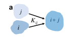
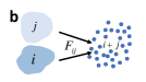
Figure 1: Aggregation (a) and shattering (b) of clusters.

In this article we consider collision-controlled fragmentation, which is thought to be responsible e.g. for interstellar dust clouds and planetary rings Krapivsky and Ben-Naim (2003); Brilliantov et al. (2009, 2015); Stadnichuk et al. (2015). We explore the extreme version, namely a complete shattering of two colliding partners into monomers (see Fig. 1). Symbolically $[i]+[j]\xrightarrow{F_{i,j}}\underbrace{[1]+[1]+\ldots[1]}_{i+j}$ where $F_{i,j}$ quantifies the shattering rate. It has been shown Brilliantov et al. (2015) that this shattering model is rather generic—realistic impact models with a strong dominance of small debris over the large ones yield the same resulting cluster size distribution $n_{k}$. Following Brilliantov et al. (2015), we assume that the shattering and aggregation kernels are proportional,

$$F_{i,j}=\lambda K_{i,j}.$$ (2)

The parameter $\lambda$ characterizes the relative frequency of collisions leading to merging and shattering.

Incorporating the shattering process with the shattering kernel (2) into Eqs. (1) we arrive at

$$\frac{dn_{1}}{dt} = -n_{1}\sum\limits_{i=1}^{\infty}K_{1,i}n_{i}+\frac{\lambda}{2}\sum\limits_{i=2}^{\infty}\sum\limits_{j=2}^{\infty}(i+j)K_{i,j}n_{i}~{}n_{j}$$ (3)

$$+ \lambda n_{1}\sum\limits_{j=2}^{\infty}jK_{1,j}n_{j}$$

$$\frac{dn_{k}}{dt} = \frac{1}{2}\sum\limits_{i=1}^{k-1}K_{i,k-i}n_{i}n_{k-i}-(1+\lambda)n_{k}\sum\limits_{i=1}^{\infty}K_{k,i}n_{i}.$$

Shattering leads to the increase of monomers explaining the gain terms in the first equation (3) and it leads to the decrease of the density of other clusters explaining the loss term in the second equation.

A microscopic analysis is needed to establish how the kernels $K_{i,j}$ and $F_{i,j}$ depend on the masses, see e.g. Brilliantov et al. (2015, 2009). The kernels are always symmetric, $K_{i,j}=K_{j,i}$, and in most applications homogeneous functions of $i$ and $j$. Aggregation-shattering equations (3) for the generalized product kernels, $K_{i,j}=(ij)^{\mu}$, have been investigated in Brilliantov et al. (2015). A more general family of kernels, $K_{i,j}=i^{\nu}j^{\mu}+i^{\mu}j^{\nu}$, is often used in studies of aggregation, see e.g. Ref. Connaughton et al. (2017) where a source of monomers and sink of large clusters was present. We shall focus on a special case of $\mu=-\nu$,

$$K_{i,j}=i^{a}j^{-a}+i^{-a}j^{a},$$ (4)

which is also known as a generalized Brownian kernel Krapivsky and Connaughton (2012). Below we always assume that $a\leq 1$, since aggregation equations with kernel (4) satisfying $a>1$ become ill-defined due to instantaneous gelation Hendriks et al. (1983); van Dongen (1987); Brilliantov and Krapivsky (1991); Laurençot (1999); Malyushkin and Goodman (2001); Ball et al. (2011).

Time-dependent analytical solutions of Eqs. (3) have been found Brilliantov et al. (2015) only for the simplest case of a constant kernel ($a=0$). The steady-state solutions have been obtained for a wider class of models, including irreversible aggregation model with a monomer source Hayakawa (1987), aggregation-fragmentation model with the generalized product kernel Brilliantov et al. (2015) and for a somewhat similar open system with a source of monomers and collisional evaporation of clusters with the kernel $K_{i,j}=i^{\nu}j^{\mu}+i^{\mu}j^{\nu}$ Connaughton et al. (2017). An open aggregating system with the same coagulation kernel driven by input of monomers and supplemented with removal of large clusters has been studied in Ball et al. (2012). Stable oscillations have been numerically observed Ball et al. (2012) in this system with finite number of cluster species. For a closed system consisting of monomers, dimers, trimers and exited monomers, stable oscillations of concentrations have been reported Bykov and Gorban (1987). Steady chemical oscillations have been also found in a simple dimerization model (see e.g. Stich et al. (2013) and references therein).

Here we consider closed systems undergoing aggregation and shattering processes, so there are no sources and sinks of monomers and clusters. The aggregation and shattering kernels are described by Eqs. (4) and (2). One expects that in the closed system with two opposite processes and without sinks and sources, a steady state is achieved. This is indeed the case when the parameter $a<1/2$. Surprisingly, for $1/2<a\leq 1$ and small values of $\lambda$, a steady state is not reached and instead cluster concentrations undergo never-ending oscillations.

An important advantage of the kernel (4) is the possibility to apply highly efficient numerical methods. Here we exploit a fast and accurate method of time-integration of Smoluchowski-type kinetic equations developed in recent studies Matveev et al. (2015); Smirnov et al. (2016); Matveev et al. (2016); Chaudhury et al. (2014); Hackbusch (2006, 2007), that has been adopted for the discrete distribution of cluster sizes. In our simulations we use up to $N_{\rm eq}=2^{19}\equiv 524,288$ equations; in practice, we choose $N_{\rm eq}$ in such a way, that the further increase of $N_{\rm eq}$ does not impact the simulation results for $n_{k}$ within the numerical accuracy .

We confirm the efficiency and accuracy of the above fast-integration method for constant kernels ($a=0$), comparing the numerical results with the available analytical solutions Brilliantov et al. (2015) and find that the smaller the parameter $\lambda$ the longer it takes for the system to reach the steady state, see the Supplementary Material (SM). This tendency persists for the kernels (4) with $a>0$. We also observe that for $a<1/2$ the system arrives at its steady-state with a monotonic evolution of the concentrations $n_{k}(t)$. Moreover, the steady-state distribution of the cluster concentrations agrees fairly well with analytical results for $n_{k}$ derived below. Figure 2 illustrates the numerical solution for steady-state distribution for $a=0.05$ and $a=0.1$ and different values of the shattering parameter $\lambda$. In the language of dynamical systems Strogatz (1994) we conclude that the system possesses a stable fixed point with the steady-state cluster size distribution.

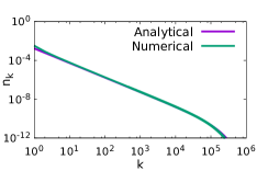
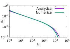
Figure 2: Comparison of the steady-state numerical solution of Eqs. (3) for the kernel (4) with $a=0.05$, $\lambda=0.003$ (top) and $a=0.1$, $\lambda=0.02$ (bottom) with the analytical steady-state solution, Eq. (9).

For $1/2<a\leq 1$, we also observed the relaxation to a steady state for sufficiently large $\lambda$, the relaxation occurs through oscillations for smaller $\lambda$, and when $\lambda<\lambda_{c}(a)$ the oscillations persist. We detected oscillations independently of the initial conditions.

The dynamic of the system described by Eqs. (3) and (4) is invariant with respect to re-scaling of the total mass density $M=\sum_{k=1}^{\infty}kn_{k}$ (see the SM). Below we report simulation results for the stepwise initial distribution

$$n_{k}(0)=\begin{cases}0.1&k=1,\ldots,10\\ 0&k>10\end{cases}$$ (5)

and we also simulated the evolution starting with mono-disperse initial condition, $n_{k}(0)=M\delta_{1,k}$, with the same mass $M=5.5$. Unless explicitly stated, the results below correspond to the initial condition (5).

In Figs. 3–4 we demonstrate the time dependence of the cluster density $N(t)=\sum_{k=1}^{\infty}n_{k}(t)$. Figure 3 shows that in the range $0.6\leq a\leq 0.8$ and $0.001\leq\lambda\leq 0.01$, the oscillations become more pronounced when $a$ increases and $\lambda$ decreases.

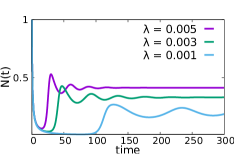
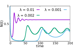
Figure 3: Time dependence of the clusters density, $N(t)$, for $a=0.7$ (top) and $a=0.75$ (bottom) and different $\lambda$. For all these systems damped oscillations are found that tend to a steady-state. The oscillations become more pronounced with increasing $a$ and decreasing $\lambda$.

In Fig. 4 we show oscillating solutions for $N(t)$ for $0.9<a\leq 1$. The new feature observed in Fig. 4 is the emergence of stationary oscillations. All cluster concentration $n_{k}(t)$ perform these stable oscillations; the form of the oscillations depends on the cluster size and the amplitude decreases with the increasing size, see Fig. 5. Figure 6, demonstrates that the system reaches a limit cycle  which does not depend on the total mass or initial conditions.

Our results indicate the existence of a critical value of $\lambda_{c}(a)$ such that for $\lambda<\lambda_{c}(a)$ the steady-state solution is no longer stable and instead the system approaches to a limit cycle. Although for $a<0.9$ we have observed only damped oscillations, we believe that stationary oscillations would emerge for all $a\geq 1/2$ but the required values of $\lambda$ are too small. When $\lambda$ is small, a huge number of equations is needed to achieve a requested precision. For example, for the simulations presented in Fig. 3 already $200,000$ equations have been used. For systems with $\lambda<\lambda_{c}$ for $a<0.9$, one needs to solve $N_{\rm eq}>10^{6}$ nonlinear ODEs which is a formidable task even when fast numerical methods are applied (see the SM).

Our major observations may be summarized as follows:

1. When $a<1/2$, there exists a single stable fixed point for all values of $\lambda$; the steady state distribution of cluster sizes $n_{k}$ corresponds to this fixed point.

2. When $1/2<a\leq 1$ and $\lambda>\lambda_{c}(a)$, the system has a single stable fixed point; it may be a stable focus, resulting in dumped oscillations.

3. When $1/2<a\leq 1$ and $\lambda<\lambda_{c}(a)$, the system has an attractive limit cycle.

In the $1/2<a\leq 1$ range, the above assertions are conjectural and require further verification.

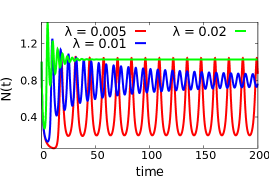
Figure 4: Time dependence of the cluster density, $N(t)$ for $a=0.9$ and different $\lambda$. For small $\lambda<\lambda_{c}(a)$ stable oscillations emerge.

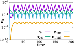
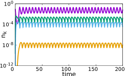
Figure 5: Stationary oscillations of the aggregate concentrations for $a=0.95$ (top) and $a=1$ (bottom) and $\lambda<\lambda_{c}(a)$. The shape of the oscillations depends on the aggregates’ size; the amplitude of the oscillations decreases with the size.

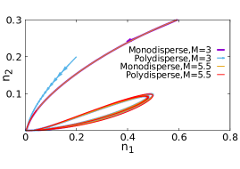
Figure 6: Limit cycle for the steady-state oscillations in terms of $n_{1}(t)$ and $n_{2}(t)$ for $a=0.95$ and $\lambda=0.005$. For the total mass density $M=5.5$ the initial conditions are mono-disperse, $n_{k}=M\delta_{1,k}$ and stepwise, (5). For $M=3$ the initial and current values of $n_{1}(t)$ and $n_{2}(t)$ are re-scaled accordingly. The relaxation to the unique limit cycle is clearly visible.

To find the steady-state cluster size distribution we set $dn_{1}/dt=0$ and $dn_{k}/dt=0$ in Eqs. (3) and solve the resulting infinite system of algebraic equations. Introducing the generating functions ${\cal C}_{\pm a}(z)=\sum_{k\geq 1}k^{\pm a}n_{k}z^{k}$, we transform (3) into

$${\cal C}_{a}(z)\,{\cal C}_{-a}(z) + (1+\lambda)zn_{1}(M_{a}+M_{-a})$$

$$= (1+\lambda)\left(M_{a}{\cal C}_{-a}(z)-M_{-a}{\cal C}_{a}(z)\right).$$

where ${\cal C}_{\pm a}(1)=M_{\pm a}$. Setting $z=1$ in Eq. (Oscillations in aggregation-shattering processes) yields

$$M_{a}M_{-a}=\frac{1+\lambda}{1+2\lambda}n_{1}(M_{a}+M_{-a}).$$ (7)

To analyze the tail of the size distribution, i.e. $n_{k}$ for $k\gg 1$, we exploit the methods described e.g. in Krapivsky et al. (2010); Krapivsky and Connaughton (2012) in the context of similar problems. Recalling that when $a=0$ the tail is $n_{k}\simeq\lambda\pi^{-1/2}k^{-3/2}e^{-\lambda^{2}k}$ for $k\gg 1$, see Brilliantov et al. (2015), suggests that $n_{k}\simeq Ck^{-\tau}e^{-\omega k}$ for $k\gg 1$, with some constants $C$, $\tau$ and $\omega$. Expanding the generating functions ${\cal C}_{\pm a}(z)$ near $z^{\prime}\to 1-0$, where $z^{\prime}=z/z_{0}$ and $z_{0}=e^{\omega}$, we get

$${\cal C}_{\pm a}(z)={\cal C}_{\pm a}(z_{0})+C\Gamma(1\pm a-\tau)(1-z^{\prime})^{\tau\mp a-1}.$$ (8)

Here $\Gamma(x)$ is the gamma function and we assume that ${\cal C}_{a}(z_{0})=\sum_{k\geq 1}k^{a}n_{k}z_{0}^{k}<\infty$ exists for given $a$ and $\tau$. If we substitute the above ${\cal C}_{\pm a}(z)$ into Eq. (Oscillations in aggregation-shattering processes) we obtain terms with different powers of the factor $(1-z^{\prime})$. To satisfy this equation we equate to zero all these terms separately. In this way we obtain equations for the zero-order terms of $(1-z^{\prime})$, and the terms of the order of $(1-z^{\prime})^{\tau\pm a-1}$. Combining these equations with Eq. (7) we find $\tau=3/2$ and $\omega\simeq\lambda^{2}$, and finally the amplitude $C=M\lambda\pi^{-1/2}$ (see SM for details). Thus the tail of the cluster size distribution reads

$$n_{k}\simeq\lambda\pi^{-1/2}Mk^{-3/2}e^{-\lambda^{2}k}\qquad{\rm for}\qquad k\gg 1.$$ (9)

In the above analysis we assume that ${\cal C}_{a}(z_{0})$ exists. This is a consistent assumption when $a<1/2$, but fails for $a\geq 1/2$ (see the SM) thereby manifesting a qualitative change in the system dynamics, which we indeed observe in simulations.

To conclude, we investigated numerically and analytically a system of particles undergoing aggregation and collision-controlled shattering (the complete fragmentation into monomers). We considered spatially homogeneous well-mixed systems characterized by the aggregation kernel $K_{i,j}=(i/j)^{a}+(j/i)^{a}$ and shattering kernel $F_{i,j}=\lambda K_{i,j}$. For $a<1/2$, we obtained an analytical solution for the steady-state cluster size distribution and confirmed numerically the relaxation of the size distribution to this steady-state form. For $a\geq 1/2$, the temporal behavior drastically depends on the shattering constant $\lambda$: When $\lambda>\lambda_{c}(a)$ the system relaxes to a steady-state through damped oscillations, while for $\lambda<\lambda_{c}(a)$ oscillations become stationary and persist forever (Figs. 4–6).

Using the language of dynamical systems our observations can be reformulated as follows: (i) for $a<1/2$ the governing system of ODEs possesses a single stable fixed point for all values of $\lambda$, (ii) for $1/2\leq a\leq 1$, the system has a single stable fixed point (which may be a stable focus) when $\lambda\geq\lambda_{c}(a)$, and (iii) for $1/2\leq a\leq 1$ and $\lambda<\lambda_{c}(a)$ the system possesses a stable limit cycle.

Limit cycles may arise already for two coupled ODEs Strogatz (1994). Still, the emergence of stable oscillations in a closed system comprising an infinite number of species and undergoing aggregating and shattering is striking. To the best of our knowledge this phenomenon has not been previously observed and a relaxation towards the steady state was believed to be the only possible scenario.

The work was supported by the Russian Science Foundation, grant 14-11-00806.

Supplemental Material: Oscillations in aggregation-shattering processes

Numerical versus analytical solutions for the constant kernels

Figure 7 illustrates the application of the fast-integration method for the case of constant aggregation and shattering kernels ($a=0$). The numerical solution approaches to the steady-state solution which is known analytically Brilliantov et al. (2015):

$$n_{k}=\frac{N}{\sqrt{4\pi}}\left(1+\lambda\right)\left[\frac{2n_{1}}{(1+\lambda)N}\right]^{k}\,\frac{\Gamma(k-\frac{1}{2})}{\Gamma(k+1)}\,.$$

Here $n_{1}=\lambda/(1+\lambda)$ is the stationary density of monomers and $N=2\lambda/(1+2\lambda)$ is the stationary density of clusters. The above distribution refers to the case of unit mass density, $M=1$, the general case is obtained by multiplying the above densities by $M$. For $\lambda\ll 1$ and $k\gg 1$, the above exact distribution simplifies to

$$n_{k}=\frac{\lambda}{\sqrt{\pi}}\,e^{-\lambda^{2}k}\,k^{-3/2}\,.$$ (10)

Figure 7 demonstrates the high accuracy of the numerical method and the intuitively obvious feature that the smaller the parameter $\lambda$ the longer it takes for the system to reach the steady state (when $\lambda=0$, the steady state is never reached).

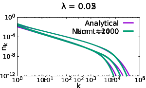
Figure 7: Comparison of the numerical solution with the analytical steady-state solution Brilliantov et al. (2015) for the constant kernel $K_{i,j}=1$ and monodisperse initial conditions, $n_{k}(0)=M\delta_{1,k}$ with $M=1$, for $\lambda=0.05$ (left panel) and $\lambda=0.02$ (right panel).

Limit Cycles of kinetic equations with homogeneous kernels

One must be careful while talking about limit cycles for kinetic equations with homogeneous kernels. By definition, a limit cycle is an isolated closed trajectory; this means that its neighboring trajectories are not closed — they spiral either towards or away from the limit cycle Strogatz (1994). After this definition, we are usually told that limit cycles can only occur in nonlinear systems; in a linear system exhibiting oscillations closed trajectories are neighbored by other closed trajectories. We also learn that a stable limit cycle is one which attracts all neighboring trajectories. A system with a stable limit cycle can exhibit self-sustained oscillations Strogatz (1994).

Consider a dynamical system that may be written as

$$\frac{dn_{k}}{dt}=F_{k}({\bf n}),\quad k\geq 1$$ (11)

where ${\bf n}=(n_{1},n_{2},n_{3},\ldots)$ and $F_{k}({\bf n})$ is given in our case by Eqs. (3) and (4) of the main text. It is important to note that the reaction terms $F_{k}({\bf n})$ are strictly quadratic polynomials for all $k$, and this fact alone leads to the conclusion that limit cycles in the dynamical system (11) are impossible. Indeed, Eqs. (11) are invariant under the transformation

$$t\to T/M,\quad n_{k}\to MN_{k}$$ (12)

namely after this transformation Eqs. (11) become

$$\frac{dN_{k}}{dT}=F_{k}({\bf N})$$ (13)

with the same functions $F_{k}$. Therefore if the dynamical system (11) possesses a limit cycle, we can slightly perturb it by choosing $M=1+\epsilon$ with $|\epsilon|\ll 1$ and obtain another limit cycle implying that a closed trajectory is not isolated and hence it is not a limit cycle. (More generally, the dynamical system (11) in which $F_{k}({\bf n})$ for all $k$ are homogeneous polynomials of any degree does not have limit cycles.)

We now recall that our dynamical system actually admits an integral of motion, namely the mass density is conserved:

$$\sum_{j\geq 1}jn_{j}=1.$$ (14)

In Eq. (14) we have set the mass density to unity; if the mass density is equal to $M$, we can make the transformation (12) and then the mass density will be equal to unity.

The original dynamical system (11) was considered in the (infinite-dimensional) quadrant

$$\mathbb{R}_{+}^{\infty}=\{(n_{1},n_{2},n_{3},\ldots)|n_{1}\geq 0,n_{2}\geq 0,n_{3}\geq 0,\ldots\}.$$ (15)

But it is more appropriate to reduce (11) to the phase space which is an intersection of (14) and (15). Plugging $n_{1}=1-\sum_{j\geq 2}jn_{j}$ into (11) with $k\geq 2$ we obtain

$$\frac{dn_{k}}{dt}=G_{k}({\bf n}),\quad k\geq 2.$$ (16)

The functions $G_{k}({\bf n})$ are still quadratic polynomials, but not strictly quadratic. For example, the term $n_{1}n_{2}$ turns into $n_{2}-\sum_{j\geq 2}jn_{j}n_{2}$.

The dynamical system (16) is defined on

$$\left\{(n_{2},n_{3},\ldots)|n_{2}\geq 0,n_{3}\geq 0,\ldots;\sum_{j\geq 2}jn_{j}\leq 1\right\}$$ (17)

which is the (infinite-dimensional) simplex. This dynamical system may admit genuine limit cycles. Hence all dynamical systems (11) and (15) with different masses $M$ are equivalent to the generic one, given by Eqs. (16) and (17). In other words, systems with different masses $M$ may be mapped on each other by simple re-scaling. Most of our simulations have been done for the stepwise initial distribution of the cluster sizes,

$$n_{j}(0)=\begin{cases}0.1&1\leq j\leq 10\\ 0&j>10,\end{cases}$$ (18)

with the total mass $M=5.5$. To illustrate that our limit cycle is unique (up to the numerical precision) we also consider the total mass of $M=3$ and mono-disperse initial conditions $n_{k}(0)=M\delta_{1,k}$. In Fig. 6 of the main text it is demonstrated that the closed trajectories of the $n_{1}(t)-n_{2}(t)$ plane coincide for different masses and initial conditions after the appropriate re-scaling. This proves numerically the existence of true limit cycle in the system of interest.

Analytical approach for the stationary distribution

To find the steady-state distribution of the aggregates sizes, one needs to put $\dot{n}_{1}=\dot{n}_{k}=0$ into the left-hand side of Eqs. (3) and (4) of the main text and solve the following infinite system of algebraic equations:

$$n_{1}\sum\limits_{i=1}^{\infty}K_{1i}n_{i}-\frac{\lambda}{2}\sum_{i=2}^{\infty}\sum_{j=2}^{\infty}(i+j)K_{i,j}n_{i}~{}n_{j}-\lambda n_{1}\sum_{j=2}^{\infty}jK_{1,j}n_{j}=0$$ (19)

$$\frac{1}{2}\sum\limits_{i=1}^{k-1}K_{i,k-i}n_{i}n_{k-i}-(1+\lambda)n_{k}\sum\limits_{i=1}^{\infty}K_{k,i}n_{i}=0,\qquad\qquad k\geq 2.$$

We will apply the method of generating functions that has proved its efficiency for similar problems Krapivsky et al. (2010); Leyvraz (2003); Krapivsky and Connaughton (2012). Namely, we introduce the generating functions ${\cal C}_{\pm a}(z)$ and moments $M_{\pm a}$:

$${\cal C}_{\pm a}(z)=\sum_{k=1}^{\infty}k^{\pm a}n_{k}z^{k}\qquad M_{\pm a}=\sum_{k=1}^{\infty}k^{\pm a}n_{k},$$ (20)

Multiplying (19) by $z^{k}$ and summing over all $k\geq 1$ we arrive at

$${\cal C}_{a}(z){\cal C}_{-a}(z)+(1+\lambda)zn_{1}(M_{a}+M_{-a})-(1+\lambda)\left(M_{a}{\cal C}_{-a}(z)+M_{-a}{\cal C}_{a}(z)\right)=0.$$ (21)

Specializing (21) to $z=1$ and taking into account that ${\cal C}_{\pm a}(1)=M_{\pm a}$ we obtain

$$M_{a}M_{-a}=\frac{1+\lambda}{1+2\lambda}n_{1}(M_{a}+M_{-a}).$$ (22)

The tail of the size distribution can be extracted from the asymptotic behavior of the generation functions ${\cal C}_{a}(z)$. We consider separately the cases of $a<1/2$ and $a>1/2$.

Kernels with $a<1/2$. The tail (10) arising in the context of the model with constant kernel, $a=0$, in the case when additionally $\lambda\ll 1$, suggests that generally steady-state distribution may have a similar tail,

$$n_{k}\simeq Ck^{-\tau}e^{-\omega k}\qquad\qquad{\rm for}\qquad\qquad k\gg 1,$$ (23)

for kernels with $a>0$. The amplitudes $C$ and $\omega$ and the exponent $\tau$ are yet unknown functions of $\lambda$ and $a$. The generation functions may be expanded near $z^{\prime}\to 1-0$, where $z^{\prime}=z/z_{0}$ and $z_{0}=e^{\omega}$. One seeks the expansions in the form Krapivsky et al. (2010); Krapivsky and Connaughton (2012)

$${\cal C}_{a}(z) = {\cal C}_{a}(z_{0})+C\Gamma(1+a-\tau)(1-z^{\prime})^{\tau-a-1}$$ (24)

$${\cal C}_{-a}(z) = {\cal C}_{-a}(z_{0})+C\Gamma(1-a-\tau)(1-z^{\prime})^{\tau+a-1},$$ (25)

where $\Gamma(x)$ is the gamma function and we assume that ${\cal C}_{a}(z_{0})=\sum_{k\geq 1}k^{a}n_{k}z_{0}^{k}<\infty$ exists for given $a$ and $\tau$. If we substitute the above ${\cal C}_{\pm a}(z)$ into Eq. (Oscillations in aggregation-shattering processes) we obtain terms with different powers of the factor $(1-z^{\prime})$. To satisfy this equation we equate to zero all these terms separately. Then the zero-order terms of $(1-z^{\prime})$ yield

$${\cal C}_{a}(z_{0}){\cal C}_{-a}(z_{0})-(1+\lambda)\left(M_{a}{\cal C}_{-a}(z_{0})+M_{-a}{\cal C}_{a}(z_{0})\right)+(1+\lambda)z_{0}n_{1}(M_{a}+M_{-a})=0.$$ (26)

Similarly, the terms of the order $(1-z^{\prime})^{\tau\pm a-1}$ imply the relations

$${\cal C}_{\mp a}(z_{0})\Gamma(1\pm a-\tau)-(1+\lambda)M_{\mp a}\Gamma(1\pm a-\tau)=0.$$ (27)

Finally, the rest of the terms should satisfy

$$C^{2}\Gamma(1+a-\tau)\Gamma(1-a-\tau)(1-z^{\prime})^{2\tau-2}-(1+\lambda)z_{0}n_{1}(M_{a}+M_{-a})(1-z^{\prime})=0.$$ (28)

This equation is consistent when

$$2\tau-2=1\qquad\qquad{\rm or}\qquad\qquad\tau=\frac{3}{2}\,.$$ (29)

The exponent $\tau$ is therefore universal (independent on $a$ and $\lambda$). Now we substitute the relations

$${\cal C}_{\mp a}(z_{0})=(1+\lambda)M_{\mp a},$$ (30)

which follow from Eq. (27) into Eq. (26) to yield

$$M_{a}M_{-a}=\frac{z_{0}}{1+\lambda}n_{1}(M_{a}+M_{-a}).$$ (31)

From Eqs. (31) and (7) then follows,

$$z_{0}=e^{\omega}=\frac{(1+\lambda)^{2}}{(1+2\lambda)}.$$ (32)

The ansatz (23) is expected to work only when $\lambda\ll 1$. In this limit (32) gives $\omega\simeq\lambda^{2}-2\lambda^{3}+\ldots\simeq\lambda^{2}$, so the amplitude $\omega$ is independent on $a$. Thus the tail of the cluster size distribution reads

$$n_{k}\simeq\frac{C}{k^{3/2}}e^{-\lambda^{2}k}\qquad\qquad{\rm for}\qquad\qquad k\gg 1.$$ (33)

An order-of-magnitude estimate for the constant $C$ may be done as follows. We assume that the distribution (33), which holds true for $k\gg 1$ may be also used for $k\sim 1$, so that

$$\sum_{k=1}^{\infty}kn_{k}\simeq\int_{1}^{\infty}\frac{C}{k^{1/2}}e^{-\lambda^{2}k}dk\simeq\frac{C\sqrt{\pi}}{\lambda}=1,$$ (34)

that is, $C\simeq\lambda/\sqrt{\pi}\sim\lambda$.

Kernels with $a>1/2$. Applying the same analysis as above for $a\geq 1/2$, one arrives at Eqs. (26)–(28), which however do not lead to consistent results. Indeed, from Eq. (28) it follows that $\tau=3/2$, but ${\cal C}_{a}(z_{0})$ does not exist for $a\geq 1/2$, so that Eq. (27) may not be satisfied to cancel the terms corresponding to the factor $(1-z^{\prime})^{\tau+a-1}$.

Although the above approach fails to make consistent asymptotic estimates for $a\geq 1/2$, our results for $a<1/2$ and the results of Ref. Connaughton et al. (2017) for a similar system motivate as to exploit a hypothesis, that for $a\geq 1/2$, the distribution of cluster size has the following form for $k\gg 1$: $n_{k}\simeq Ck^{-3/2}e^{-\lambda^{\beta}k}$; it will be used below for the further analysis.

Truncating an infinite system of equations by a finite number of equations

The standard problem of numerical solution of Smoluchowski equations is how to approximate an infinite system of equations by a finite one. When fragmentation is lacking, as in common Smoluchowski equations, the average size of aggregates infinitely grows which imposes a principle time limit for the modeled processes. Contrary, in the case of interest, the fragmentation of aggregates precludes the formation of very large clusters even for infinitely long time. Therefore the number of equations may be finite. Moreover, using the results for the steady-state distribution, one can estimate the number of equations needed to describe the system with a given degree of accuracy. Below we show, how the solutions of a formally infinite system (3) of the main text may be adequately represented by these of a finite system.

Using Eqs. (3) of the main text, we write for the concentration $n_{k}(t)$ for $2\leq k\leq L$:

$$\frac{dn_{k}}{dt}=\frac{1}{2}\sum\limits_{i=1}^{k-1}K_{i,k-i}n_{i}n_{k-i}-(1+\lambda)n_{k}\sum\limits_{i=1}^{L}K_{k,i}n_{i}-\left\{(1+\lambda)n_{k}\sum\limits_{i=L+1}^{\infty}K_{k,i}n_{i}\right\}.$$ (35)

Taking into account that for $a\leq 1$ and $k<L<i$

$$K_{i,k}=\left(\frac{i}{k}\right)^{a}+\left(\frac{k}{i}\right)^{a}\leq i^{a}+k^{a}<i+i=2i$$

and applying the steady-state distribution,

$$n_{k}\simeq Ck^{-\frac{3}{2}}e^{-\lambda^{\beta}k}$$

we estimate the factor in the curled bracket in (35) as

$$\sum_{i=L+1}^{\infty}K_{i,k}n_{i}<2\sum_{i=L+1}^{\infty}in_{i}\sim\int_{L}^{\infty}xCx^{-\frac{3}{2}}e^{-\lambda^{\beta}x}dx\sim CL^{\frac{1}{2}}\frac{\text{Erfc}(\sqrt{\lambda^{\beta}L})}{\sqrt{\lambda^{\beta}L}}.$$

If the quantity $\lambda^{\beta}L$ is large, one can make a further simplification, using the asymptotic relation $\text{Erfc}(x)\sim e^{-x^{2}}/x$, which yields,

$$\sum_{i=L+1}^{\infty}K_{i,k}n_{i}<C\frac{e^{-\lambda^{\beta}L}}{\lambda^{\beta}L^{\frac{1}{2}}}<\varepsilon.$$ (36)

Hence, if we choose the number of equations $L=N_{\rm eq}(\lambda)$ such that the above expression is smaller than $\varepsilon\ll 1$ we can safely skip the term in the curled brackets in Eq. (35) to obtain:

$$\frac{dn_{k}}{dt}=\frac{1}{2}\sum\limits_{i=1}^{k-1}K_{i,k-i}n_{i}n_{k-i}-(1+\lambda)n_{k}\sum\limits_{i=1}^{N_{\rm eq}}K_{ki}n_{i},$$

that is, the solution of an infinite system may be approximated with any desired accuracy by the solution of a finite system with the appropriately chosen number of equations. In practice, we started with the number of equations estimated from Eq. (36) for $\beta=2$ and $C\sim\lambda$, as for the steady-state distribution for $a<1/2$ and checked, whether the simulation results keep unchanged (within the machine precision) when the number of equations increases. For the most of studied systems the appropriate number of equations was about $N_{\rm eq}=150,000$.

References

- Flory (1953) P. J. Flory, Principles of Polymer Chemistry (Cornell University Press, 1953).
- Krapivsky et al. (2010) P. L. Krapivsky, S. Redner, and E. Ben-Naim, A kinetic view of statistical physics (Cambridge University Press, 2010).
- Leyvraz (2003) F. Leyvraz, Physics Reports 383, 95 (2003).
- Poeschel et al. (2003) T. Poeschel, N. V. Brilliantov, and C. Frommel, Biophys. J. 85, 3460 (2003).
- Shrivastava (1982) R. C. Shrivastava, J. Atom. Sci. 39, 1317 (1982).
- Dorogovtsev and Mendes (2003) S. N. Dorogovtsev and J. F. F. Mendes, Evolution of networks: From biological nets to the Internet and WWW (Oxford University Press, 2003).
- Zakharov et al. (2012) V. E. Zakharov, V. S. L’vov, and G. Falkovich, Kolmogorov Spectra of Turbulence I: Wave Turbulence (Springer, 2012).
- Brilliantov et al. (2015) N. V. Brilliantov, P. L. Krapivsky, A. Bodrova, F. Spahn, H. Hayakawa, V. Stadnichuk, and J. Schmidt, PNAS 112, 9536 (2015).
- Stadnichuk et al. (2015) V. Stadnichuk, A. Bodrova, and N. V. Brilliantov, Int. J. Mod. Phys. B 29, 1550208 (2015).
- Cuzzi et al. (2010) J. N. Cuzzi, J. A. Burns, S. Charnoz, R. N. Clark, J. E. Colwell, L. Dones, L. W. Esposito, G. Filacchione, R. G. French, M. M. Hedman, et al., Science 327, 1470 (2010).
- Brilliantov et al. (2009) N. V. Brilliantov, A. Bodrova, and P. L. Krapivsky, J. Stat. Mech.: Theory and Experiment 2009, P06011 (2009).
- Esposito (2006) L. Esposito, Planetary Rings (Cambridge University Press, 2006).
- Strogatz (1994) S. H. Strogatz, Nonlinear Dynamics and Chaos (Addison Wesley publishing company, 1994).
- Krapivsky and Ben-Naim (2003) P. L. Krapivsky and E. Ben-Naim, Phys. Rev. E 68, 021102 (2003).
- Connaughton et al. (2017) C. Connaughton, A. Dutta, R. Rajesh, and O. Zaboronski, EPL 117, 10002 (2017).
- Krapivsky and Connaughton (2012) P. L. Krapivsky and C. Connaughton, J. Chem. Phys. 136, 204901 (2012).
- Hendriks et al. (1983) E. M. Hendriks, M. H. Ernst, and R. M. Ziff, J. Stat. Phys. 31, 519 (1983).
- van Dongen (1987) P. G. J. van Dongen, J. Phys. A 20, 1889 (1987).
- Brilliantov and Krapivsky (1991) N. V. Brilliantov and P. L. Krapivsky, J. Phys. A: Math. Gen. 24, 4787 (1991).
- Laurençot (1999) P. Laurençot, Nonlinearity 12, 229 (1999).
- Malyushkin and Goodman (2001) L. Malyushkin and J. Goodman, Icarus 150, 314 (2001).
- Ball et al. (2011) R. C. Ball, C. Connaughton, T. H. M. Stein, and O. Zaboronski, Phys. Rev. E 84, 011111 (2011).
- Hayakawa (1987) H. Hayakawa, J. of Phys. A 20, L801 (1987).
- Ball et al. (2012) R. C. Ball, C. Connaughton, P. P. Jones, R. Rajesh, and O. Zaboronski, Phys. Rev. Lett. 109, 168304 (2012).
- Bykov and Gorban (1987) V. I. Bykov and A. N. Gorban, Chem. Eng. Sci. 42, 1249 (1987).
- Stich et al. (2013) M. Stich, C. Blanco, and D. Hochberg, Physical Chemistry Chemical Physics 15, 255 (2013).
- Matveev et al. (2015) S. A. Matveev, A. P. Smirnov, and E. E. Tyrtyshnikov, J. Comput. Phys. 282, 23 (2015).
- Smirnov et al. (2016) A. P. Smirnov, S. Matveev, D. Zheltkov, E. E. Tyrtyshnikov, et al., Procedia Computer Science 80, 2141 (2016).
- Matveev et al. (2016) S. A. Matveev, D. A. Zheltkov, E. E. Tyrtyshnikov, and A. P. Smirnov, J. Comput. Phys. 316, 164 (2016).
- Chaudhury et al. (2014) A. Chaudhury, I. Oseledets, and R. Ramachandran, Computers & Chemical Engineering 61, 234 (2014).
- Hackbusch (2006) W. Hackbusch, Computing 78, 145 (2006).
- Hackbusch (2007) W. Hackbusch, Numerische Mathematik 106, 627 (2007).
- Ben-Naim and Krapivsky (2008) E. Ben-Naim and P. L. Krapivsky, Phys. Rev. E 77, 061132 (2008).