Charged Randall-Sundrum black holes in Higher Dimensions

M. Meiers, L. Bovard and R.B. Mann

Department of Physics & Astronomy, University of Waterloo, Waterloo, Ontario N2L 3G1, Canada

We extend some solutions for black holes in the Randall-Sundrum theory with a single brane. We consider a generalised version of the extremal black hole on the brane in $n+1$ dimensions and determine an asymptotic value of the geometry for large black holes.

1 Introduction

Some time ago Randall and Sundrum proposed [1] a novel approach to add an extra unexperienced dimension to use in quantum gravity by considering a $(4+1)$ dimensional world where non-gravitational physics is constrained to a $(3+1)$ dimensional hypersurface (or brane), while gravitational effects are allowed to propagate through a bulk $5$ dimensional AdS spacetime. At low energies, the theory reduces to 4D general relativity at large distances compared with the AdS length $\ell$.

In understanding whether and how the RS model is capable of recovering the strong field predictions of general relativity for bulk dimensions $N>4$ [2], localized black hole solutions provide a useful tool. While a considerable amount of numerical work suggests such solutions exist (at least for small black holes) [3][4], there is still no analytic solution, except in $(2+1)$ dimensions [5]. However it is known that there are no asymptotically flat black hole solutions to general relativity in $(2+1)$ dimensional spacetime, leading to the conclusion that the existence of this solution is due to quantum corrections from the dual Conformal Field Theory. These corrections turn what would be a conical singularity classically into a regular horizon [6]. While inducing a negative cosmological constant on the brane yields braneworld black hole solutions that are similar to those of $(2+1)$ dimensional AdS general relativity [7], large black holes are not localized on the brane.

In an attempt to make progress on this issue, Kaus and Reall (KR) [8], considered an extreme black hole in (4+1) dimensions charged with respect to an electromagnetic field on the brane. By examining the extremal solution one can take advantage of symmetries of the near horizon geometry in the bulk solution. This approach has the bulk equations reduce to ordinary differential equations that integrate to yield a 1-parameter family of solutions. Solving the Israel junction conditions to obtain the gravitational effect on the brane yields a relationship between this parameter and the charge on the brane, which then serves to label this family of solutions.

Here we seek to find extremal black hole solutions in $N=(n+1)$ bulk dimensions that contains an electromagnetic field on an $n$-dimensional brane. We intend to determine whether the structure exhibited by the $(4+1)$ dimensional extremal black hole is unique to that dimension of the brane and whether pathologies exist in higher dimensional braneworld theories. There is hope that there is some robustness in the properties found in models in the style of Randall and Sundrum, as seen in other higher dimensional extensions of other models [9] [10]. For properties that are robust, one could hope to better understand them in the large $N$ limit where general relativity reduces to a simpler model [11]. There may also be advantages of allowing $N$ to take continuous values and look at limits where the deviation of $N$ from an integer value becomes small.

We proceed by employing a warped product ansatz for the near-horizon metric whose space transverse to the horizon is a sphere of dimension $D$ (as opposed to 2 in KR) and solve the resulting field equations in this context. By solving the Israel junction conditions on the brane we are able to determine the gravitational affect of the brane on the overall geometry. For $D=2$ the structure of the Israel junction conditions determine the specific geometry of the spacetime, $k=-1$ [8]. These arguments can then be continued to higher dimensions to again restrict to branes of the form $AdS_{2}\times S^{D}$.

Using our ansatz we find equations of motion that can be solved with a single parameter family of solutions. The action on an electromagnetically charged brane is then used to put junction conditions on the extrinsic curvature in the bulk. We then look at the possible solutions in greater depth and delve into uncovering the structural relations between the charge and radius of the black hole. We observe how the entropy measured in the brane and bulk differ, and construct an argument to find that for dimensions greater than $5$ the scaling of the entropy of small black holes is fundamentally different.

We begin with generalizing the derivations [8] of the equations of motion and junction conditions for higher dimension. Following our equations we look at the analytic solutions possible before we consider numeric solutions. We conclude by discussing the properties of these solutions and examining the entropy scaling observed.

2 The Equations of Motion

The near horizon geometry of a static extreme black hole can be written in the warped product form [12]

$$ds^{2}=A^{2}(z)d\Sigma^{2}+dz^{2}+R^{2}(z)d\Omega_{D}^{2}$$ (1)

with $d\Sigma^{2}=-dt^{2}+S(k)^{2}dr^{2}$, where $S(0)=1$, $S(-1)=\sin(t)$ and $S(1)=\sinh(t)$ . Both $t$ and $r$ have been made unitless by using either the (A)dS radius $\ell$ for $k=\pm 1$ or some arbitrary length scale for $k=0$. The co-ordinate $z$ corresponds to the transverse distance from the brane and $d\Omega_{D}^{2}$ is the line element on $S^{D}$, with $N-1=D+2$ the dimension of the brane, and $N=D+3$ the overall dimension of the bulk.

The corresponding bulk Einstein field equations are given by

$$R_{\mu\nu}=-\frac{(D+2)}{\ell^{2}}g_{\mu\nu}$$ (2)

and inserting the black hole ansatz (1) into the field equations yields

$$\frac{k}{A^{2}}-\frac{1}{A^{2}}\left(\frac{dA}{dz}\right)^{2}-\frac{D}{AR}\frac{dA}{dz}\frac{dR}{dz}-\frac{1}{A}\frac{d^{2}A}{dz^{2}} =-\frac{(D+2)}{\ell^{2}}$$

$$\frac{2}{A}\frac{d^{2}A}{dz^{2}}+\frac{D}{R}\frac{d^{2}R}{dz^{2}} =\frac{(D+2)}{\ell^{2}}$$ (3)

$$\frac{(D-1)}{R^{2}}-\frac{(D-1)}{R^{2}}\left(\frac{dR}{dz}\right)^{2}-\frac{2}{AR}\frac{dA}{dz}\frac{dR}{dz}-\frac{1}{R}\frac{d^{2}R}{dz^{2}} =-\frac{(D+2)}{\ell^{2}}$$

which reduce to the 5-dimensional version of [8] with $D=2$. By denoting $R=\ell\,\rho(z/\ell)$ and $A=\ell\,\alpha(z/\ell)$ we can re-write these equations as

$$\frac{k-\alpha^{\prime 2}}{\alpha^{2}}-\frac{D\alpha^{\prime}\rho^{\prime}}{\alpha\rho} -\frac{\alpha^{\prime\prime}}{\alpha}=-(D+2)$$

$$\frac{2\alpha^{\prime\prime}}{\alpha}+\frac{D\rho^{\prime\prime}}{\rho} =(D+2)$$ (4)

$$\frac{(D-1)(1-\rho^{\prime 2})}{\rho^{2}}-\frac{2\alpha^{\prime}\rho^{\prime}}{\alpha\rho} -\frac{\rho^{\prime\prime}}{\rho}=-(D+2)$$

where the prime denotes the deriviative with respect to $x=z/\ell$. The Hamiltonian constraint is given by combining these three equations to eliminate the second order derivatives.

$$\frac{2(k-\alpha^{\prime 2})}{\alpha^{2}}-\frac{4D\alpha^{\prime}\rho^{\prime}}{\alpha\rho}+\frac{D(D-1)(1-\rho^{\prime 2})}{\rho^{2}}=-(D+2)(D+1)$$ (5)

Since the horizon is compact in the bulk, the D- sphere of the geometry must contract to a point. As a result $\rho(z/l)$ must vanish somewhere; this location can be chosen to be $z=0$ without loss of generality. Requiring that the equations of motions are smooth at $z=0$ then implies

$$\alpha(z/\ell)=\sqrt{\frac{\beta}{D+2}}+\frac{\beta+k}{D+1}\left(\frac{D+2}{\beta}\right)^{1/2}\left(\frac{z}{\ell}\right)^{2}$$

$$+\frac{\beta+k}{D+1}\left(\frac{(D-1)\beta-(3D+5)k}{(D+1)(D+3)}\right)\left(\frac{D+2}{\beta}\right)^{3/2}\left(\frac{z}{\ell}\right)^{4}\ldots$$ (6)

$$\rho(z/\ell)=\frac{z}{\ell}+\frac{(D-1)\beta-2k}{D(D+1)}\left(\frac{D+2}{\beta}\right)\left(\frac{z}{\ell}\right)^{3}$$

$$+\frac{\left(D^{3}+D^{2}+19D+3\right)\beta^{2}+4\left(5D^{2}+16D+3\right)k\beta+4\left(6D^{2}+13D+3\right)k^{2}}{D^{2}(D+1)^{2}(D+3)}\left(\frac{D+2}{\beta}\right)^{2}\left(\frac{z}{\ell}\right)^{5}\ldots$$ (7)

where $\alpha(0)=\sqrt{\frac{\beta}{D+2}}$ for some positive $\beta$.

3 Junction Conditions

The $n=N-1$ dimensional brane action is given by

$$S_{\text{brane}}=\int d^{n}z\sqrt{-h}\left(-\sigma-\frac{1}{16\pi G_{n}}F_{ij}F^{ij}\right)$$ (8)

where $h_{ij}$ is the induced metric on the brane, $\sigma$ is the brane tension, $G_{n}$ is Newton’s constant on the brane, and $F$ is the electromagnetic field on the brane. The tension of the brane is given by $\sigma=(N-2)/4\pi G_{N}\ell$ and $G_{n}=(N-3)G_{N}/2\ell$ [7]. The action results in an energy-momentum tensor

$$T_{ab}=\frac{1}{4\pi G_{n}}F_{ai}{F_{b}}^{i}-h_{ab}\left(\sigma+\frac{1}{16\pi G_{n}}F_{ij}F^{ij}\right)$$ (9)

$$T=-\frac{N-5}{16\pi G_{n}}F_{ij}F^{ij}-(N-1)\sigma$$ (10)

localized on the brane. Employing the junction conditions (see (30) as in the appendix) and assuming that the brane is located at $z=z_{0}$ is $\mathbb{Z}_{2}$ symmetric about $z_{0}$ and thus $K_{ab}(z_{0}^{+})=-K_{ab}(z_{0}^{-})$ we find

$$K_{ab}(z_{0}) =\frac{8\pi G_{N}}{2}\left(\frac{1}{N-2}\left(-\frac{N-5}{16\pi G_{n}}F_{ij}F^{ij}-(N-1)\sigma\right)h_{ab}+\frac{-1}{4\pi G_{n}}F_{ai}{F_{b}}^{i}\right.$$

$$+\left.h_{ab}\left(\sigma+\frac{1}{16\pi G_{n}}F_{ij}F^{ij}\right)\right)$$

$$=\frac{-4\pi G_{N}\sigma}{N-2}h_{ab}+\frac{G_{N}}{G_{n}}\left(\frac{3}{4(N-2)}h_{ab}F_{ij}F^{ij}-F_{ai}{F_{b}}^{i}\right)$$

$$=\frac{-1}{\ell}h_{ab}+\frac{2\ell}{N-3}\left(\frac{3}{4(N-2)}F_{ij}F^{ij}h_{ab}-F_{ai}{F_{b}}^{i}\right)$$ (11)

which up to a sign convention reduces down to the $N=5$ case of [8]. We assume the electromagnetic field to be spherically symmetric and purely electric, yielding

$$\star_{n}F=Q_{D}\mathrm{d}\Omega_{D}$$ (12)

where $\star_{n}$ is the Hodge dual in $n$ dimensions, $F$ is the Faraday differential form, and $d\Omega_{D}$ is the volume form on a $D$ sphere. Given that for a $2-$form $\omega$ on a Lorentzian manifold the Hodge dual satisfies $\star_{n}\star_{n}\omega=-\omega$ the sign is $(-1)^{k(n-k)}s$ (where $s$ is the sign of our metric so (-1) and $k$ is the rank of the tensor) we find that the electromagnetic field strength is given by

$$F=-\star_{n}\star_{n}F=-Q_{D}\star_{n}(\mathrm{d}\Omega_{D})=-Q_{D}\frac{S(k)A^{2}(z_{0})}{R^{D}(z_{0})}\mathrm{d}t\wedge\mathrm{d}r$$ (13)

We can use the definition of extrinsic curvature on our chosen metric and normal vector to write $K_{ab}=\left.-\frac{1}{2}\partial_{z}(g_{ab})\right|_{z=z_{0}}$. The junction conditions (3) then become

$$\left.\frac{1}{2}\partial_{z}(g_{ab})\right|_{z=z_{0}} =\frac{1}{\ell}h_{ab}+\frac{2\ell}{N-3}\left(\frac{3}{2(N-2)}\frac{Q_{D}^{2}}{R^{2D}(z_{0})}h_{ab}+\frac{Q_{D}^{2}A^{2}(z_{0})}{R^{2D}(z_{0})}\left(\delta_{a}^{t}\delta_{b}^{t}-S(k)^{2}\delta_{a}^{r}\delta_{b}^{r}\right)\right)$$ (14)

which reduce to two independent constraints

$$\frac{\alpha^{\prime}(z_{0}/\ell)}{\alpha(z_{0}/\ell)}=1-\frac{2N-7}{(N-3)(N-2)}\frac{q_{D}^{2}}{\rho^{2D}(z_{0}/\ell)}\qquad\frac{\rho^{\prime}(z_{0}/\ell)}{\rho(z_{0}/\ell)}=1+\frac{3}{(N-3)(N-2)}\frac{q_{D}^{2}}{\rho^{2D}(z_{0}/\ell)}$$ (15)

in terms of $\alpha$ and $\rho$, where $q_{D}=Q/\ell^{D-1}$. These conditions can be combined and rearranged to the form

$$3\frac{\alpha^{\prime}(z_{0}/\ell)}{\alpha(z_{0}/\ell)}+(2D-1)\frac{\rho^{\prime}(z_{0}/\ell)}{\rho(z_{0}/\ell)}=2(D+1)\qquad q_{D}=\rho^{D}(z_{0})\sqrt{\frac{D}{2}\left(\frac{\rho^{\prime}(z_{0}/\ell)}{\rho(z_{0}/\ell)}-\frac{\alpha^{\prime}(z_{0}/\ell)}{\alpha(z_{0}/\ell)}\right)}$$ (16)

The Hamiltonian constraint can also be evaluated at $z=z_{0}$ to give

$$\frac{7D-2}{D^{2}(D+1)}\frac{q_{D}^{4}}{\rho^{4D}(z_{0}/\ell)}+\frac{2(D-2)}{D}\frac{q_{D}^{2}}{\rho^{2D}(z_{0}/\ell)}+\frac{D(D-1)}{\rho^{2}(z_{0}/\ell)}=\frac{-2k}{\alpha^{2}(z_{0}/\ell)}$$ (17)

and, for $D\geq 2$ each term on the left hand side is positive; hence $k=-1$, eliminating the other choices. There may be interest in the D=1 case where $k$ does not have these restrictions from the Hamiltonian constraint.

4 Solutions

We can now restrict ourselves to $k=-1$ which affords us two exact solutions. We will first look at the properties of the two exact solutions and then explore the remainder of the parameter space.

The two analytic solutions are a generalization of those found in [8]. For the first case we set $\beta=D+2$ or $\alpha(0)=1$ and find

$$\alpha(z/\ell)=\cosh(z/\ell)\qquad\rho(z/\ell)=\sinh(z/\ell)$$ (18)

However the first condition in (16) requires either $z_{0}/\ell=\mathrm{arctanh}\left(\frac{1}{3}(2D-1)\right)$ or $z_{0}/\ell=\mathrm{arctanh}(1)=\infty$. The former solution is not real for $D\geq 2$. For the latter solution both $\alpha=\infty$ and $\rho=\infty$, forcing $q_{D}=0$. Under this (17) becomes $D(D-1)=2$ for $D\geq 2$, and so this analytic solution requires $D=2$. As we will see in the following sections, for $D>2$ there are solutions with $z_{0}/\ell=\infty$, which result from $\alpha(0)<1$; however they are not analytic.

The second exact solution sets $\beta=1$ which results in $\alpha$ being constant

$$\alpha(z/\ell)=\frac{1}{\sqrt{D+2}}\qquad\rho(z/\ell)=\sqrt{\frac{D}{D+2}}\sinh\left(\sqrt{\frac{D+2}{D}}\frac{z}{\ell}\right).$$ (19)

Using the Israel junction conditions, we find that we can express $q_{D},\rho_{0}$ exactly as

$$z_{0} =\ell\sqrt{\frac{D}{D+2}}\mathrm{arccoth}\left(\frac{2D+2}{2D-1}\sqrt{\frac{D}{D+2}}\right)$$ (20)

$$q_{D} =\sqrt{\frac{D(D+1)}{2D-1}}\left((2D-1)\sqrt{\frac{D}{4D^{2}+11D-2}}\right)^{D}$$ (21)

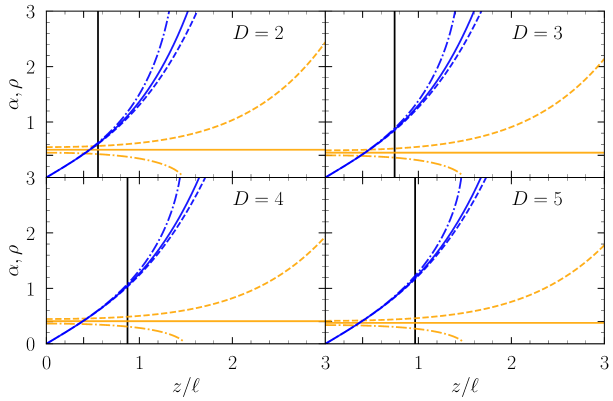
Figure 1: Plots of the behaviour of $\rho(z/\ell)$ (blue) and $\alpha(z/\ell)$ (orange). The dimension of the hypersphere $D$ runs from $2$ to $5$ starting in the top left then proceeding across and then down. $\beta$ takes the values of $1/2$ (dot dashed), $1$ (solid) and $2$ (dashed). For $\beta<1$ we place a vertical line at the location of the brane to demonstrate that $z_{0}$ occurs before $\alpha=0$.

For general values of $\beta$, we will rely on numeric techniques. As our equations of motion are singular at $0$, we must rely on the expansions (2) and (2) taken to $\mathcal{O}(\left(\frac{z}{\ell}\right)^{22})$ which can be evaluated at $z=10^{-16}\ell$ to generate initial conditions. In general, we find two kinds of behaviour surrounding the case of constant $\alpha$ which can be seen in figure (1). For $\beta>1$ we must have $\alpha(0)>\sqrt{1/(D+2)}$, and we find that $\alpha$ and $\rho$ tend towards being proportional to $e^{z/\ell}$ for large $z$, as illustrated in figure (2). Conversely, for $\beta<1$ we see new behaviour where $\alpha$ monotonically decreases to $0$, for some finite $z_{1}$, at which point $\rho$ also diverges. A calculation of the Kretschmann scalar indicates that there is a curvature singularity at $z_{1}$. This singularity would be naked if the brane, and therefore the $\mathbb{Z}_{2}$ flip across it was not placed before it. In all our simulations we find $z_{0}<z_{1}$ meaning the area of the solution is not reached in the full RS model.

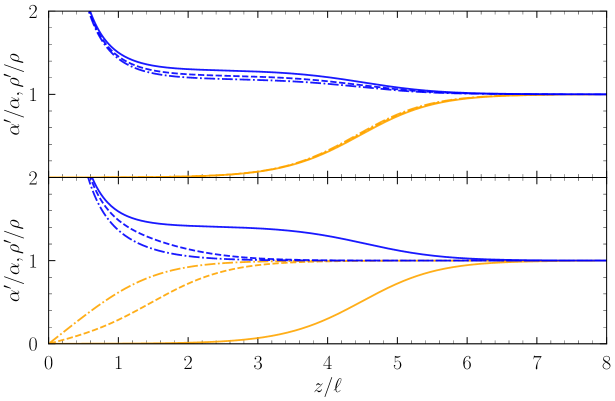
Figure 2: $\rho^{\prime}/\rho$ (blue) and $\alpha^{\prime}/\alpha$ (orange) for various $D=3,4,5$ (solid, dashed, dash dot) with fixed $\beta$ (top), and various $\beta=1.001,1.2,2$ (solid, dashed, dash dot) with fixed $D$ (bottom). This behaviour persists for all $\beta>1$ tested. We conclude $\alpha(z/\ell),\rho(z/\ell)\propto e^{z/\ell}$ for large $z/\ell$.

The equations of motion always have solutions and the junction conditions eliminate additional regions parameter space present in these solutions. For $D=2$ the limiting cases are the first analytic solutions (18) and (19) described above [8], and for all $\alpha(0)<1$ solutions can be found. However for $D>2$ this is no longer the case. We find that the value of the upper bound of $\alpha(0)$ is not easily characterized. In figure (3) we plot $z_{0}/\ell$ for various values of $\alpha(0)$ and we can see that $z_{0}$ seems to diverge for some value of $\alpha(0)$ that decreases with $D$, see table (1) for the value of the bounding $\alpha(0)$. Below this bound, we find that solutions exist for all positive $\alpha(0)$ with $z_{0}\propto\alpha(0)$ for small initial values.

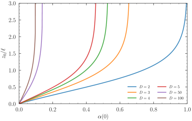
Figure 3: The location of the brane $z_{0}/\ell$ of differing initial radii of the $AdS_{2}$ space for various spherical dimensions.

Spherical Dimension ($D=N-3$)	Bound on $\alpha(0)$
2	1
3	$\approx 0.66$
4	$\approx 0.53$
5	$\approx 0.46$
6	$\approx 0.42$
7	$\approx 0.38$
8	$\approx 0.35$
50	$\approx 0.14$
100	$\approx 0.10$

Table 1: The bounding value of $\alpha(0)$ of higher bulk dimension

We now switch to a parametrization in terms of the more physically natural parameter of charge, $q_{D}$ to find the behaviour of $\alpha(z_{0}),\rho(z_{0})$ for large $z_{0}$. We can use the scaling of $q_{D}$ with $\ell$ to guess that

$$\alpha(z_{0})=\gamma_{(\alpha,D)}q_{D}^{1/D-1}\qquad\rho(z_{0})=\gamma_{(\rho,D)}q_{D}^{1/D-1}\qquad\text{for }q_{D}\gg 1$$ (22)

where $\gamma_{(\alpha,D)}$ and $\gamma_{(\rho,D)}$ are constants dependent on dimension. Figure (4) demonstrates this behaviour for the first few dimensions and figure (5) shows the behaviour of the numerically found constants. We note that for extremely small $q_{D}$ both $\alpha(z_{0})/q^{1/(D-1)}$ and $\rho(z_{0})/q^{1/(D-1)}$ diverge, but the scale is incredibly small.

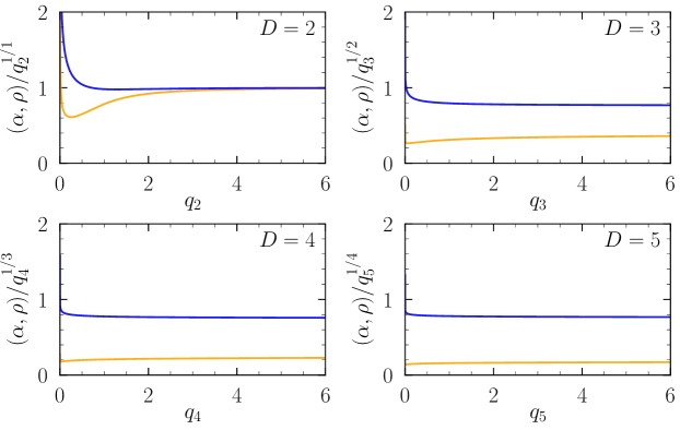
Figure 4: The ratios between $\alpha(z_{0}/\ell)$ (orange) and $\rho(z_{0}/\ell)$ (blue) to $q_{D}^{1/(D-1)}$. The dimension of the hypersphere $D$ runs from $2$ to $5$ starting in the top left then proceeding across and then down.

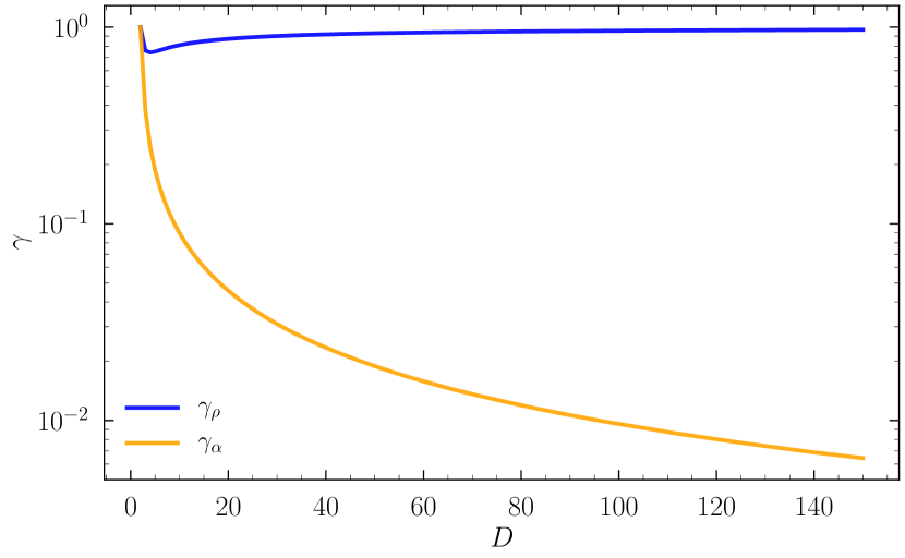
Figure 5: Numerical ratio, $\gamma$, between $\alpha(z_{0}/\ell)$ (orange) and $\rho(z_{0}/\ell)$ (blue) and $q_{D}^{1/(D-1)}$ for increasing dimension $D$.

5 Entropy of Small black holes

Figure (3) suggests that for small $z_{0}$, $z_{0}\propto\alpha(0)$. As such, by their expansions (2) and (2) to first order, $\alpha(z_{0})$ and $\rho(z_{0})$ all scale as $\alpha(0)$. From the second relation of (16), we find that $\rho(z_{0})\propto q_{D}^{2/(2D-1)}$ in the regime of small $z_{0}$ where $\rho^{\prime}(z_{0})\approx 1$ and $\alpha^{\prime}(z_{0})=0$. Consequently, by transitivity $z_{0},\alpha(z_{0})$ and, $\alpha(0)\propto q_{D}^{2/(2D-1)}$. Thus $\alpha(z_{0})/q_{D}^{1/(D-1)}\propto q_{D}^{-1/(2D-1)(D-1)}$, which demonstrates the divergence of that ratio for $q_{D}\rightarrow 0$. Identical scaling applies to $\rho(z_{0})$ and accounts for the similar behaviour of its ratio for small $q_{D}$. We then find

$$S_{D+3}\propto\int_{0}^{z_{0}}\mathrm{d}z\rho^{D}(z/\ell)\approx\frac{\ell}{D+1}\rho^{D+1}(z_{0})\propto\ell q_{D}^{2(D+1)/(2D-1)}$$

unlike the expected scaling $\sim q_{D}^{{D}/{D-1}}$ from (22). It is worth noting that unlike the specific case of $D=2$, for general $D$ we have $\frac{D}{D-1}\neq\frac{2(D+1)}{2D-1}$ and as a result we find for small $z_{0}$ that our entropy scaling changes for $D>2$.

6 Conclusion

We have obtained extremally charged black hole solutions for a higher dimensional Randall Sundrum models. We find a dimensional robustness to brane world black holes that is commensurate with previous $D=2$ results [8]. While the equations of motion for the near horizon geometry allow for the space to have a subspace that is any 2D Lorentzian manifold, only the choice of $\text{AdS}_{2}$ allow for satisfaction of the junction conditions. Under these constraints we find solutions in any dimension.

However we find that some properties of black holes for the $D=2$ case are unique. For black holes that are large compared to the AdS radius we find an identical scaling dependence of entropy with respect to charge. However in contrast to this, small black holes break the scaling behaviour except for the specific case $D=2$. This change in entropy scaling may be expected as the RS model can only recover perturbative Newtonian gravity at which the scales are large compared to $\ell$. For $D=2$ [8] it may just be a coincidence that such matching holds for smaller black holes.

In the large $q_{D}$ regime we also found that the constants of proportionality for the scaling relations are no longer equal to one another, with both becoming less than unity. As seen in Figure  (5) it appears the scaling for the AdS’ subspace size to $q_{D}$ falls off in the large dimension limit. The spherical subspace’s scaling distinquishes itself by initially decreasing from unity of the initial $N=5$ case but slowly recovering becoming the larger contribution to the size of the space.

An exploration into how to better obtain the numerically found constant of proportionality for entropy for given dimension or a formulation of the dependence would also be advantageous. The divergence from the standard entropy scaling relations leaves room for inquiry concerning on if and how these new relations extend to non-static geometry systems.

Junction Condition

We generalize the junction conditions made for N=5 bulk in [2] to bulk spacetimes of arbitrary dimension. We make use of Israel’s technique and break up our $N$ dimensional bulk into a family of $N-1$ dimensional sub-manifolds described by the coordinates $x^{a}$, and a normal distance from a particular surface $z$. To distinguish between tensors which lie in the full space or only on the hypersurfaces, we will use Greek for the former and Latin for the latter. Let the metric in the bulk take the form

$$\mathrm{d}s^{2}=h_{ab}(x,z)\mathrm{d}x^{a}\mathrm{d}x^{b}+\mathrm{d}z^{2}$$

where $h_{ab}$ lies in the tangent space of the sub-manifolds which encapsulates the information in the intrinsic metric. We can also bring $h$ into the full space to act as a projection metric to find the surface parallel components of tensors in the tangent space of the bulk. To bring $h$ up, let us define $n^{\mu}=\delta_{z}^{\mu}$ which describes the direction normal to each surface. The projection tensor thus takes the form

$$\tilde{h}_{\mu\nu}=g_{\mu\nu}-n_{\mu}n_{\nu}.$$ (23)

We will use the tilde to bring an element of the tangent space of the $N-1$ dimensional structure into the tangent space of the $N$ dimensional space via an inclusion map. The data encoded in $h$ could be employed to find the intrinsic curvature on the surface, but we have more interest in connecting the bulk’s curvature to the $h$. In order to do this connection, we need a means to measure the bending of the surface in the larger space. This bending is measured using the extrinsic curvature

$$K_{\mu\nu}=\tilde{h}_{\mu}^{\alpha}\tilde{h}_{\nu}^{\beta}\nabla_{\alpha}n_{\beta}$$

which clearly is tangential to the hypersurface, and although subtle in this form, it can be shown to be symmetric. There are a few results which also follow from our choice of the Gauss Normal gauge. The first uses that $n_{\mu}n^{\mu}=1$ for all coordinates which implies that $0=\frac{1}{2}\nabla_{\alpha}(n_{\mu}n^{\mu})=n^{\mu}\nabla_{\alpha}(n_{\mu})$ . Consequentially,

$$K_{\mu\nu}=\tilde{h}_{\mu}^{\alpha}\tilde{h}_{\nu}^{\beta}\nabla_{\alpha}n_{\beta}=\tilde{h}_{\mu}^{\alpha}(\delta^{\beta}_{\nu}-n^{\beta}n_{\nu})\nabla_{\alpha}n_{\beta}=\tilde{h}_{\mu}^{\alpha}(\nabla_{\alpha}n_{\nu}-n_{\nu}n^{\beta}\nabla_{\alpha}n_{\beta})=\tilde{h}_{\mu}^{\alpha}\nabla_{\alpha}n_{\nu}.$$ (24)

which allows us to not need the second projection. In fact, because $n^{\mu}=\delta_{z}^{\mu}$ implying $\partial_{\mu}n^{\nu}=0$ and $g_{z\mu}=\delta^{z}_{\mu}$ one can conclude

$$n^{\mu}\nabla_{\mu}n_{\nu}=n^{\mu}\left(\frac{1}{2}\partial_{z}g_{\mu\nu}\right)=\left(\frac{1}{2}\partial_{z}g_{z\nu}\right)=0.$$

As a result of this property, we can further simplify the extrinsic curvature to require no projections

$$K_{\mu\nu}=\tilde{h}_{\mu}^{\alpha}\nabla_{\alpha}n_{\nu}=(\delta^{\alpha}_{\mu}-n_{\mu}n^{\alpha})\nabla_{\alpha}n_{\nu}=\nabla_{\mu}n_{\nu}.$$ (25)

Finally, we make note of two identities

$$\nabla_{\mu}\tilde{h}_{\alpha}^{\beta}=-K_{\mu\alpha}n^{\beta}-{K_{\mu}}^{\beta}n_{\alpha}$$ (26)

which follow from (25) and the Leibniz rule, and another for the Lie derivative of the extrinsic curvature

$$\mathcal{L}_{n}K_{\mu\nu}=n^{\lambda}\nabla_{\lambda}K_{\mu\nu}+K_{\lambda\nu}\nabla_{\mu}n^{\lambda}+K_{\mu\lambda}\nabla_{\nu}n^{\lambda}=n^{\lambda}\nabla_{\lambda}K_{\mu\nu}+2K_{\mu\lambda}{K_{\nu}}^{\lambda}.$$ (27)

Using these tools, a well-known exercise yields the Gauss-Codazzi relation

$${\tilde{R}^{(N-1)\,\mu}}_{\;\;\;\qquad\lambda\alpha\beta}=\left({K_{\alpha}}^{\mu}\tilde{h}^{\rho}_{\beta}-{K_{\beta}}^{\mu}\tilde{h}^{\rho}_{\alpha}\right)K_{\rho\lambda}+\tilde{h}^{\mu}_{\mu^{\prime}}\tilde{h}^{\lambda^{\prime}}_{\lambda}\tilde{h}^{\alpha^{\prime}}_{\alpha}\tilde{h}^{\beta^{\prime}}_{\beta}{R^{\mu^{\prime}}}_{\lambda^{\prime}\alpha^{\prime}\beta^{\prime}}.$$ (28)

and the relation

$$\mathcal{L}_{n}K_{\alpha\beta}={\tilde{R}^{(N-1)}}_{\qquad\alpha\beta}+2{K_{\alpha}}^{\lambda}K_{\beta\lambda}-8\pi G_{N}\tilde{h}_{\alpha}^{\alpha^{\prime}}\tilde{h}_{\beta}^{\beta^{\prime}}T_{\alpha^{\prime}\beta^{\prime}}+\left(\frac{N-1}{l^{2}}+\frac{8\pi G_{N}}{N-2}T\right)\tilde{h}_{\alpha\beta}.$$ (29)

Thus, if we posit that there exists a infinitesimal surface of non zero energy momentum, we can treat $T_{\alpha\beta}$ as the distribution $\delta(z)T_{\alpha\beta}$. Integrating z from $(-\epsilon,\epsilon)$, under the reasonable assumption of a finite discontinuity for all other terms, we find in the limit as $\epsilon$ tends to 0

$$K_{\alpha\beta}(z=0^{+})-K_{\alpha\beta}(z=0^{-})=8\pi G_{N}\left(\frac{1}{N-2}T\tilde{h}_{\alpha\beta}-\tilde{h}_{\alpha}^{\alpha^{\prime}}\tilde{h}_{\beta}^{\beta^{\prime}}T_{\alpha^{\prime}\beta^{\prime}}\right)$$ (30)

which constitute the Israel junction conditions.

References

- [1] L. Randall and R. Sundrum, “An alternative to compactification,” Phys. Rev. Lett., vol. 83, pp. 4690–4693, Dec 1999.
- [2] R. Gregory, Braneworld Black Holes, pp. 259–298. Berlin, Heidelberg: Springer Berlin Heidelberg, 2009.
- [3] H. Kudoh, T. Tanaka, and T. Nakamura, “Small localized black holes in a braneworld: Formulation and numerical method,” Phys. Rev. D, vol. 68, p. 024035, Jul 2003.
- [4] H. Yoshino, “On the existence of a static black hole on a brane,” Journal of High Energy Physics, vol. 2009, no. 01, p. 068, 2009.
- [5] R. Emparan, G. T. Horowitz, and R. C. Myers, “Exact description of black holes on branes,” Journal of High Energy Physics, vol. 2000, no. 01, p. 007, 2000.
- [6] R. Emparan, A. Fabbri, and N. Kaloper, “Quantum black holes as holograms in ads braneworlds,” Journal of High Energy Physics, vol. 2002, no. 08, p. 043, 2002.
- [7] R. Emparan, G. T. Horowitz, and R. C. Myers, “Exact description of black holes on branes ii: comparison with btz black holes and black strings,” Journal of High Energy Physics, vol. 2000, no. 01, p. 021, 2000.
- [8] A. Kaus and H. S. Reall, “Charged randall-sundrum black holes and = 4 super yang-mills in ads 2 s 2,” Journal of High Energy Physics, vol. 2009, no. 05, p. 032, 2009.
- [9] V. Asnin, D. Gorbonos, S. Hadar, B. Kol, M. Levi, and U. Miyamoto, “High and low dimensions in the black hole negative mode,” Classical and Quantum Gravity, vol. 24, no. 22, p. 5527, 2007.
- [10] B. Kol and E. Sorkin, “Black-brane instability in an arbitrary dimension,” Classical and Quantum Gravity, vol. 21, no. 21, p. 4793, 2004.
- [11] G. Giribet, “Large limit of dimensionally continued gravity,” Phys. Rev. D, vol. 87, p. 107504, May 2013.
- [12] H. K. Kunduri, J. Lucietti, and H. S. Reall, “Near-horizon symmetries of extremal black holes,” Classical and Quantum Gravity, vol. 24, no. 16, p. 4169, 2007.