Electromagnetic $\delta$-function sphere

Prachi Parashar prachi.parashar@ntnu.no https://www.ntnu.edu/employees/prachi.parashar Department of Energy and Process Engineering, Norwegian University of Science and Technology, NO-7491 Trondheim, Norway Homer L. Dodge Department of Physics and Astronomy, University of Oklahoma, Norman, OK 73019 ā€ƒā€ƒ Kimball A. Milton kmilton@ou.edu http://www.nhn.ou.edu/~milton Homer L. Dodge Department of Physics and Astronomy, University of Oklahoma, Norman, OK 73019 ā€ƒā€ƒ K. V. Shajesh kvshajesh@gmail.com http://www.physics.siu.edu/~shajesh Department of Physics, Southern Illinois University-Carbondale, Carbondale, IL 62901 Department of Energy and Process Engineering, Norwegian University of Science and Technology, NO-7491 Trondheim, Norway ā€ƒā€ƒ Iver Brevik iver.h.brevik@ntnu.no http://folk.ntnu.no/iverhb Department of Energy and Process Engineering, Norwegian University of Science and Technology, NO-7491 Trondheim, Norway
Abstract

We develop a formalism to extend our previous work on the electromagnetic $\delta$-function plates to a spherical surface. The electric ($\lambda_{e}$) and magnetic ($\lambda_{g}$) couplings to the surface are through $\delta$-function potentials defining the dielectric permittivity and the diamagnetic permeability, with two anisotropic coupling tensors. The formalism incorporates dispersion. The electromagnetic Green’s dyadic breaks up into transverse electric and transverse magnetic parts. We derive the Casimir interaction energy between two concentric $\delta$-function spheres in this formalism and show that it has the correct asymptotic flat plate limit. We systematically derive expressions for the Casimir self-energy and the total stress on a spherical shell using a $\delta$-function potential, properly regulated by temporal and spatial point-splitting, which are different from the conventional temporal point-splitting. In strong coupling, we recover the usual result for the perfectly conducting spherical shell but in addition there is an integrated curvature-squared divergent contribution. For finite coupling, there are additional divergent contributions; in particular, there is a familiar logarithmic divergence occurring in the third order of the uniform asymptotic expansion that renders it impossible to extract a unique finite energy except in the case of an isorefractive sphere, which translates into $\lambda_{g}=-\lambda_{e}$.

I Introduction

Having established the surprising result that a pair of parallel neutral perfect conductors experiences an attractive force due to fluctuations in the quantum electromagnetic fieldĀ Casimir (1948), Casimir suggested that this attraction should persist for a spherical shell, and could contribute to the stabilization of the electron Casimir (1953). On the contrary, when Boyer first did the calculation, he found a repulsive resultĀ Boyer (1968), which was confirmed subsequently by many authors, for example in Refs.Ā Davies (1972); BalianĀ andĀ Duplantier (1978); MiltonĀ etĀ al. (1978); LeseduarteĀ andĀ Romeo (1996); NesterenkoĀ andĀ Pirozhenko (1998),

$$E_{\rm pcs}=\frac{0.04618}{a},$$ (1)

where $a$ is the radius of the perfectly conducting sphere (pcs). This is a rather unique result in the litany of Casimir self-energies, in that it is finite and unambiguous, resulting from precise cancellations between interior and exterior contributions and between transverse electric (TE) and transverse magnetic (TM) modes. For example, although a finite scalar Casimir self-energy for an infinitesimally thin spherical shell imposing Dirichlet boundary conditions may be unambiguously extractedĀ LeseduarteĀ andĀ Romeo (1996); BenderĀ andĀ Milton (1994); Milton (1997a), divergent terms are omitted in doing so. And for other shapes, such as rectangularĀ Lukosz (1971, 1973a, 1973b); AmbjĆørnĀ andĀ Wolfram (1983) or tetrahedral AbaloĀ etĀ al. (2012) cavities, only the interior contributions can be included, although a unique self-energy can be extracted, exhibiting a universal behavior. In these cases, well-known divergences, identified through heat-kernel analyses, remain. The situation becomes even murkier with real materials. For example, a dielectric sphere exhibits an unremovable logarithmic divergenceĀ Milton (1980); BordagĀ etĀ al. (1999), which cannot be removed even after accounting for dispersionĀ BrevikĀ andĀ Einevoll (1988); only when the speed of light is the same inside and outside the sphere is the Casimir self-energy finiteĀ BrevikĀ andĀ Kolbenstvedt (1982a, b). In the dilute limit, $\varepsilon-1\ll 1$, where $\varepsilon$ is the permittivity, a finite result in the second order of the coupling is extractable MiltonĀ andĀ JackĀ Ng (1998); BrevikĀ etĀ al. (1999)

$$E_{\rm dds}=\frac{23}{1536\pi}\frac{(\varepsilon-1)^{2}}{a}.$$ (2)

In the next order, however, the above-mentioned divergence appears.

Clearly, there are issues still to be understood involving quantum vacuum self-energies. In an effort to establish better control over the calculations and at the same time have a flexible formulation, we considered diaphanous materials modeled by $\delta$-function contributions to the electric permittivity and the magnetic permeability in Refs.Ā ParasharĀ etĀ al. (2012); MiltonĀ etĀ al. (2013a). We considered an infinitesimally thin translucent plane surface and learned that the permittivity and permeability potentials were necessarily anisotropic. Here, we adapt that formalism to spherical geometry; in addition, we regulate the frequency integrals and angular momentum sums by introducing temporal and spatial point-splitting regulators, which turned out to be extremely effective in geometries with curvature and corner divergencesĀ MiltonĀ etĀ al. (2013b, c). Specifically, we keep both temporal and spatial point-splitting cutoffs, which were proposed as a tool for a systematic analysis in the context of the principle of virtual work in Refs.Ā EstradaĀ etĀ al. (2012); FullingĀ etĀ al. (2013).

In this paper, we will work in natural units $\hbar=c=1$. In the next section, we derive general formulas for the energy (and free energy at nonzero temperature) when dispersion is present. In Sec.Ā III, we summarize the concept of the $\delta$-function potential as introduced in Ref.Ā ParasharĀ etĀ al. (2012). We obtain the non-trivial boundary conditions imposed by the $\delta$-function potentials on the fields, in the presence of a spherical boundary, from Maxwell’s equations in Sec.Ā IV, and set up Green’s dyadics for Maxwell’s equations, with the appropriate boundary (matching) conditions. In Sec.Ā V, we verify the Green’s dyadic structure by evaluating the Casimir interaction energy between two concentric $\delta$-function spheres, where the asymptotic flat plate limit, i.e. the large radius and small angle, reproduces the interaction energy between two parallel $\delta$-function plates. (This coincides with the proximity force approximation, PFA, for the spherical surfaces.) For the case of a purely electric potential, contributing only to the permittivity, and with the choice of a plasma model to represent the frequency dependence of that coupling, we analyze the resulting electromagnetic vacuum energy in Sec.Ā VI. We first analyze the self-energy of a $\delta$-function plate for both strong and finite coupling. In the strong coupling case, the divergences cancel between transverse electric and transverse magnetic mode. However, for the finite coupling case, we see a logarithmic divergence appearing in the third order of the couping parameter in addition to an inverse power of the point-splitting parameter. For the spherical shell, in the strong coupling we recover the familiar result of BoyerĀ Boyer (1968), but with a divergent term, due to the square of the curvature of the sphere, whose form depends on the precise nature of the point-splitting cutoff. This divergence is not observed in the conventional temporal point-splitting cutoff. For finite coupling, the divergence structure is more complicated, and there emerges the familiar logarithmic dependence on the cutoff, which first appears in third order in the strength of the potential. Because the scale of this logarithm is ambiguous, no unique finite part can be computed. We verify these results by computing in Sec.Ā VII, directly from the stress tensor, the pressure on the spherical shell. Finally, in Sec.Ā VIII, we see how the results are modified when both potentials, electric and magnetic, are included. Apart from strong coupling, the only possible finite case is that for isorefractivity, when the electric and magnetic coupling are equal in magnitude but opposite in sign, corresponding to $\varepsilon\mu=1$. In the Conclusion, we discuss our results in light of recent literature, which might bear on some of the issues raised here.

We have extended our study to the finite temperature analysis of a $\delta$-function shellĀ MiltonĀ etĀ al. (2017), which shows a discomforting negative entropy behavior in addition to the temperature dependent divergences. In the $T=0$ study we can avoid these subtleties and gain more insight into the divergence structure depending only on the point-splitting cutoff parameter.

II Formalism

It is convenient to consider the general finite temperature case first. The free energy, including the bulk contributions, is

$$F=-\frac{T}{2}\sum_{n=-\infty}^{\infty}\operatorname{Tr}\ln\bm{\Gamma},$$ (3)

where Green’s dyadic for a arbitrary electromagnetic system at temperature $T$ in the presence of a dispersive dielectric and diamagnetic material satisfies the differential equation

$$\bm{\Gamma}^{-1}\bm{\Gamma}=\bm{1},\quad\bm{\Gamma}^{-1}=-\frac{1}{\zeta_{n}^{2}}\bm{\nabla}\times\frac{1}{\mu(\zeta_{n})}\bm{\nabla}\times-\varepsilon(\zeta_{n}),$$ (4)

in terms of the Matsubara frequency $\zeta_{n}=2\pi nT$. The entropy is

$$S=-\frac{\partial F}{\partial T}=-\frac{F}{T}+\frac{U}{T},$$ (5)

from which we identify the internal energy

$\displaystyle U$ $\displaystyle=$ $\displaystyle\frac{T}{2}\sum_{n=-\infty}^{\infty}\zeta_{n}\frac{\partial}{\partial\zeta_{n}}\operatorname{Tr}\ln\bm{\Gamma}$ (6)
$\displaystyle=$ $\displaystyle\frac{T}{2}\sum_{n=-\infty}^{\infty}\zeta_{n}\operatorname{Tr}\bm{\Gamma}^{-1}\frac{\partial}{\partial\zeta_{n}}\bm{\bm{\Gamma}}.$

The differential equation (4) allows us to transfer the derivative to the first factor in the trace, and then subsequently that equation implies

$\displaystyle U$ $\displaystyle=$ $\displaystyle-\frac{T}{2}\sum_{n=-\infty}^{\infty}\zeta_{n}\operatorname{Tr}\bm{\Gamma}\frac{\partial}{\partial\zeta_{n}}\bm{\Gamma}^{-1}$ (7)
$\displaystyle=$ $\displaystyle-\frac{T}{2}\sum_{n=-\infty}^{\infty}\zeta_{n}\operatorname{Tr}\bm{\Gamma}\left[\frac{2}{\zeta_{n}^{3}}\bm{\nabla}\times\frac{1}{\mu(\zeta_{n})}\bm{\nabla}\times-\frac{\partial}{\partial\zeta_{n}}\varepsilon(\zeta_{n})+\frac{1}{\zeta_{n}^{2}}\bm{\nabla}\times\frac{1}{\mu^{2}(\zeta_{n})}\frac{\partial\mu(\zeta_{n})}{\partial\zeta_{n}}\bm{\nabla}\times\right]$
$\displaystyle=$ $\displaystyle T\sum_{n=-\infty}^{\infty}\operatorname{Tr}\left(\varepsilon+\frac{1}{2}\zeta_{n}\frac{\partial\varepsilon}{\partial\zeta_{n}}-\frac{1}{2\zeta_{n}}\bm{\nabla}\times\frac{1}{\mu^{2}}\frac{\partial\mu}{\partial\zeta_{n}}\bm{\nabla}\times\right)\bm{\Gamma},$

At zero temperature, this reduces to the expected general formula for a dispersive mediumĀ MiltonĀ etĀ al. (2010); Candelas (1982), where $\zeta=-i\omega$ is the imaginary frequency,

$$E=U(T=0)=\int_{-\infty}^{\infty}\frac{d\zeta}{2\pi}\left[\operatorname{Tr}\varepsilon\bm{\Gamma}+\frac{1}{2}\zeta\operatorname{Tr}\bm{\Gamma}\frac{\partial}{\partial\zeta}\varepsilon-\frac{1}{2}\frac{1}{\zeta}\bm{\nabla}\times\frac{1}{\mu^{2}}\frac{\partial\mu}{\partial\zeta}\bm{\nabla}\times\bm{\Gamma}\right],$$ (8)

which is what would be obtained by integrating the dispersive form of the energy density SchwingerĀ etĀ al. (1998),

$$u(\mathbf{r})=\frac{1}{2}\left(\frac{d}{d\zeta}(\zeta\varepsilon)E^{2}+\frac{d}{d\zeta}(\zeta\mu)H^{2}\right).$$ (9)

For the case of anisotropic permittivity and permeability, provided the corresponding tensors are invertible, the same steps, starting from either the variational approach or from the electromagnetic energy density, lead to the following expression for the internal energy,

$$U=T\sum_{n=-\infty}^{\infty}\operatorname{Tr}\left[\bm{\varepsilon}\cdot\bm{\Gamma}+\frac{1}{2}\zeta_{n}\frac{d\bm{\varepsilon}}{d\zeta_{n}}\cdot\bm{\Gamma}+\frac{1}{2\zeta_{n}}\bm{\nabla}\times\frac{d\bm{\mu}^{-1}}{d\zeta_{n}}\cdot\bm{\nabla}\times\bm{\Gamma}\right]$$ (10)

that has a readily applicable form for calculating the Casimir self-energies of single objects, while the Casimir interaction energy between two objects is more conveniently evaluated using the multiple scattering expressionĀ KennethĀ andĀ Klich (2006). It is consistent with the variational statement, at zero temperature,

$$\delta E=\int_{-\infty}^{\infty}\frac{d\zeta}{2\pi}\frac{\zeta}{2}\frac{d}{d\zeta}\operatorname{Tr}\left[\delta\bm{\varepsilon}\cdot\bm{\Gamma}-\delta\bm{\mu}^{-1}\frac{1}{\zeta^{2}}\bm{\nabla\times\Gamma\times\overleftarrow{\nabla}^{\prime}}\right].$$ (11)

From this, it is quite direct to obtain the Lifshitz formula for parallel dielectric plates, as was done in Ref.Ā SchwingerĀ etĀ al. (1978) for the pure permittivity case. The above discussion may not apply in the case of dissipation, see Refs.Ā Ginzburg (1989); BrevikĀ andĀ Milton (2008).

Henceforth we specialize to the case of zero temperature. In this paper, we will be primarily considering self-energies in addition to the interaction energy, so regulation of integrals is necessary. Then, if we use point splitting in both time and space, the Casimir energy less the bulk (empty space) contribution, is

$\displaystyle E-E_{0}$ $\displaystyle=$ $\displaystyle-\frac{1}{2}\int_{-\infty}^{\infty}\frac{d\zeta}{2\pi}e^{i\zeta\tau}\operatorname{Tr}\ln\bm{\Gamma}\,\bm{\Gamma}_{0}^{-1}$ (12)
$\displaystyle=$ $\displaystyle\frac{1}{2}\int\frac{d\zeta}{2\pi}\frac{e^{i\zeta\tau}-1}{i\tau}\int d^{3}x\Big{\langle}\mathbf{x}\Big{|}\bm{\Gamma}^{-1}\frac{d\bm{\Gamma}}{d\zeta}-\bm{\Gamma}_{0}^{-1}\frac{d\bm{\Gamma}_{0}}{d\zeta}\Big{|}\mathbf{x}+\bm{\delta}\Big{\rangle},$

where $\tau$ and $\bm{\delta}$ are infinitesimal point-splitting parameters in time and space, to be taken to zero at the end of the calculation. In the second integral above, we have integrated by parts. Substituting, from Eq.Ā (4),

$$\frac{d\bm{\Gamma}}{d\zeta}=-\bm{\Gamma}\frac{d\bm{\Gamma}^{-1}}{d\zeta}\bm{\Gamma}=\bm{\Gamma}\frac{d\bm{\varepsilon}}{d\zeta}\bm{\Gamma}+\bm{\Gamma}\frac{1}{\zeta^{2}}\bm{\nabla}\times\frac{d\bm{\mu}^{-1}}{d\zeta}\bm{\nabla}\times\bm{\Gamma}+\frac{2}{\zeta}(\bm{\Gamma+\Gamma\varepsilon\Gamma}),$$ (13)

Then, just as above, we obtain the zero-temperature, regulated form of the internal energy (10)

$$E-E_{0}=\int_{-\infty}^{\infty}\frac{d\zeta}{2\pi}\frac{e^{i\zeta\tau}-1}{i\zeta\tau}\operatorname{Tr}\left[\bm{\varepsilon\Gamma}+\frac{\zeta}{2}\frac{d\bm{\varepsilon}}{d\zeta}\bm{\Gamma}+\frac{1}{2}\frac{1}{\zeta}\bm{\nabla}\times\frac{d\bm{\mu}^{-1}}{d\zeta}\bm{\nabla}\times\bm{\Gamma}-\bm{\Gamma}_{0}\right],$$ (14)

where the trace includes a point-split integration over position.

III Electromagnetic $\delta$-function potential

The $\delta$-function potential model we use in this paper was introduced and extensively explored, for the planar geometry, in Ref.Ā ParasharĀ etĀ al. (2012).

An electromagnetic $\delta$-function potential describes an infinitesimally thin material with electric permittivity $\bm{\varepsilon}$ and magnetic permeability $\bm{\mu}$ defined in terms of a $\delta$-function,

$\displaystyle{\bm{\varepsilon}}({\bf x};\omega)$ $\displaystyle=$ šŸ+š€e​(s;ω)​Γ​(sāˆ’s0),1subscriptš€š‘’š‘ šœ”š›æš‘ subscriptš‘ 0\displaystyle{\bf 1}+{\bm{\lambda}}_{e}(s;\omega)\delta(s-s_{0}), (15a)
$\displaystyle{\bm{\mu}}({\bf x};\omega)$ $\displaystyle=$ šŸ+š€g​(s;ω)​Γ​(sāˆ’s0),1subscriptš€š‘”š‘ šœ”š›æš‘ subscriptš‘ 0\displaystyle{\bf 1}+{\bm{\lambda}}_{g}(s;\omega)\delta(s-s_{0}), (15b)

where sš‘ s represents the coordinate normal to the surface. We choose isotropic electric $\bm{\lambda}_{e}$ and magnetic $\bm{\lambda}_{g}$ susceptibilities of the material in the plane of the surface by requiring $\bm{\lambda}_{e}\equiv\text{diag}(\lambda_{e}^{\perp},\lambda_{e}^{\perp},\lambda_{e}^{||})$ and $\bm{\lambda}_{g}\equiv\text{diag}(\lambda_{g}^{\perp},\lambda_{g}^{\perp},\lambda_{g}^{||})$. The choice of isotropy in the plane of the surface ensures the separation of transverse electric (TE) and transverse magnetic (TM) modes.

In Ref.Ā ParasharĀ etĀ al. (2012), we derived the conditions on the electric and magnetic fields at the boundary of such a material starting from the first order Maxwell’s equations. We showed that a consistent set of boundary conditions on the fields only included the properties of the materials confined to the surface (shown below for a spherical $\delta$-function surface). Additional constraints on the components of the material properties transverse to the surface $\lambda^{||}$ were obtained from Maxwell’s equations that lead to a necessarily anisotropic nature of the electromagnetic properties for materials described by a $\delta$-function potential. Specifically, we found $\lambda_{e}^{||}=0$ and $\lambda_{g}^{||}=0$. One must consider these discussions in light of Refs.Ā Barton (2013); Bordag (2014). The $\lambda^{||}$ components do not appear in the boundary conditions. However, releasing the aforementioned conditions would require overconstraining the electric and magnetic fields according to Maxwell’s equations. We shall extend this discussion further in Sec.Ā V.

IV Electromagnetic $\delta$-function sphere

Consider an infinitesimally thin spherical shell at the interface of two spherically symmetric media, as shown in Fig.Ā 1.

Refer to caption
Figure 1: A $\delta$-function sphere described by electric and magnetic couplings, $\lambda_{e}$ and $\lambda_{g}$, at the interface of two spherically symmetric media.

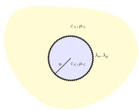
The electric permittivity and magnetic permeability for this is of the form

$\displaystyle{\bm{\varepsilon}}(r)$ $\displaystyle=$ $\displaystyle\varepsilon^{\perp}(r)\bm{1}_{\perp}+\varepsilon^{||}(r)\,\hat{\bm{r}}\hat{\bm{r}},$ (16a)
$\displaystyle{\bm{\mu}}(r)$ $\displaystyle=$ $\displaystyle\mu^{\perp}(r)\bm{1}_{\perp}+\mu^{||}(r)\,\hat{\bm{r}}\hat{\bm{r}},$ (16b)

where

$\displaystyle\varepsilon^{\perp,{||}}(r)$ $\displaystyle=$ $\displaystyle 1+(\varepsilon^{\perp,{||}}_{<}-1)\,\theta(a-r)+(\varepsilon^{\perp,{||}}_{>}-1)\,\theta(r-a)+\lambda^{\perp,{||}}_{e}\,\delta(r-a),$ (17a)
$\displaystyle\mu^{\perp,{||}}(r)$ $\displaystyle=$ $\displaystyle 1+(\mu^{\perp,{||}}_{<}-1)\,\theta(a-r)+(\mu^{\perp,{||}}_{>}-1)\,\theta(r-a)+\lambda^{\perp,{||}}_{g}\,\delta(r-a).$ (17b)

Here $\perp$ and $||$ refer to perpendicular and parallel to the radial direction $\hat{\bm{r}}$ (which defines the direction of the surface vector at each point on the sphere).

In Heaviside-Lorentz units, the monochromatic components [proportional to $\exp(-i\omega t)$] of Maxwell’s equations in the absence of charges and currents are

$\displaystyle{\bm{\nabla}}\times{\bf E}$ $\displaystyle=$ $\displaystyle i\omega{\bf B},$ (18a)
$\displaystyle-{\bm{\nabla}}\times{\bf H}$ $\displaystyle=$ $\displaystyle i\omega({\bf D}+{\bf P}),$ (18b)

which imply ${\bm{\nabla}}\cdot{\bf B}=0$, and ${\bm{\nabla}}\cdot({\bf D}+{\bf P})=0$, where ${\bf P}$ is an external source of polarization.

In the following we assume that the fields ${\bf D}$ and ${\bf B}$ are linearly dependent on the electric and magnetic fields ${\bf E}$ and ${\bf H}$ as

$\displaystyle{\bf D}({\bf x},\omega)$ $\displaystyle=$ $\displaystyle{\bm{\varepsilon}}({\bf x};\omega)\cdot{\bf E}({\bf x},\omega),$ (19a)
$\displaystyle{\bf B}({\bf x},\omega)$ $\displaystyle=$ $\displaystyle{\bm{\mu}}({\bf x};\omega)\cdot{\bf H}({\bf x},\omega).$ (19b)

A vector field can be decomposed in the basis of the vector spherical harmonics as

$${\bf V}({\bf r})=\sum_{lm}{\text{V}}^{(i)}_{lm}(r){\bf X}_{lm}^{(i)}(\theta,\phi),$$ (20)

where $i=1,2,r$ and ${\bf X}_{lm}^{(i)}\equiv({\bf\Psi}_{lm}(\theta,\phi),{\bf\Phi}_{lm}(\theta,\phi),{\bf Y}_{lm}(\theta,\phi))$ are the basis vectorsĀ BarreraĀ etĀ al. (1985):

$\displaystyle{\bf\Psi}_{lm}(\theta,\phi)$ $\displaystyle=$ $\displaystyle\frac{r}{\sqrt{l(l+1)}}\bm{\nabla}\,\mathrm{Y}_{lm}(\theta,\phi),$
$\displaystyle{\bf\Phi}_{lm}(\theta,\phi)$ $\displaystyle=$ $\displaystyle\frac{r}{\sqrt{l(l+1)}}\hat{\bf r}\times\bm{\nabla}\,\text{Y}_{lm}(\theta,\phi),$
$\displaystyle{\bf Y}_{lm}(\theta,\phi)$ $\displaystyle=$ $\displaystyle\hat{\bf r}\mathrm{Y}_{lm}(\theta,\phi).$

Maxwell’s equations in Eqs.Ā (18) thus decouple into two modes: the transverse magnetic mode (TM) involves the field components $(E^{(1)},H^{(2)},E^{(r)})$,

$\displaystyle\frac{1}{r}\frac{\partial}{\partial r}rE^{(1)}_{lm}(r)$ $\displaystyle=$ $\displaystyle\frac{\sqrt{l(l+1)}}{r}E^{(r)}_{lm}(r)+i\omega B^{(2)}_{lm}(r),$ (21a)
$\displaystyle\frac{1}{r}\frac{\partial}{\partial r}rH^{(2)}_{lm}(r)$ $\displaystyle=$ $\displaystyle i\omega\left[D^{(1)}_{lm}(r)+P^{(1)}_{lm}(r)\right],$ (21b)
$\displaystyle\frac{\sqrt{l(l+1)}}{r}H^{(2)}_{lm}(r)$ $\displaystyle=$ $\displaystyle i\omega\left[D^{(r)}_{lm}(r)+P^{(r)}_{lm}(r)\right],$ (21c)

and the transverse electric mode (TE) involves the field components $(H^{(1)},E^{(2)},H^{(r)})$,

$\displaystyle\frac{1}{r}\frac{\partial}{\partial r}rH^{(1)}_{lm}(r)$ $\displaystyle=$ $\displaystyle\frac{\sqrt{l(l+1)}}{r}H^{(r)}_{lm}(r)-i\omega\left[D^{(2)}_{lm}(r)+P^{(2)}_{lm}(r)\right],$ (22a)
$\displaystyle\frac{1}{r}\frac{\partial}{\partial r}rE^{(2)}_{lm}(r)$ $\displaystyle=$ $\displaystyle-i\omega B^{(1)}_{lm}(r),$ (22b)
$\displaystyle\frac{\sqrt{l(l+1)}}{r}E^{(2)}_{lm}(z)$ $\displaystyle=$ $\displaystyle-i\omega B^{(r)}(r).$ (22c)

IV.1 Boundary conditions

The boundary conditions on the electric and magnetic fields ${\bf E}$ and ${\bf H}$ are obtained by integrating across the $\delta$-function boundary. We get additional contributions to the standard boundary conditions at the interface of two media due to the presence of the $\delta$-function sphere. The only requirement on the the electric field ${\bf E}$ and magnetic field ${\bf H}$ is that they are free from any $\delta$-function type singularities, which is evident from the second-order differential equation of the fields. The boundary conditions on the fields are

TM TE
$\displaystyle E^{(1)}_{lm}(r)\Big{|}^{r=a+}_{r=a-}$ $\displaystyle=i\omega\lambda_{g}^{\perp}H^{(2)}_{lm}(a),$ $\displaystyle H^{(1)}_{lm}(r)\Big{|}^{r=a+}_{r=a-}$ $\displaystyle=-i\omega\lambda_{e}^{\perp}E^{(2)}_{lm}(a),$ (23a)
$\displaystyle H^{(2)}_{lm}(r)\Big{|}^{r=a+}_{r=a-}$ $\displaystyle=i\omega\lambda_{e}^{\perp}E^{(1)}_{lm}(a),$ $\displaystyle E^{(2)}_{lm}(r)\Big{|}^{r=a+}_{r=a-}$ $\displaystyle=-i\omega\lambda_{g}^{\perp}H^{(1)}_{lm}(a)$ (23b)
$\displaystyle D^{(r)}_{lm}(r)\Big{|}^{r=a+}_{r=a-}$ $\displaystyle=\frac{\sqrt{l(l+1)}}{a}\lambda_{e}^{\perp}E^{(1)}_{lm}(a),$ $\displaystyle B^{(r)}_{lm}(r)\Big{|}^{z=a+}_{z=a-}$ $\displaystyle=\frac{\sqrt{l(l+1)}}{a}\lambda_{g}^{\perp}H^{(1)}_{lm}(a).$ (23c)

We evaluate quantities that are discontinuous on the $\delta$-function sphere using the averaging prescription, introduced earlier in Refs.Ā Cavero-PelĆ”ezĀ etĀ al. (2008a, b). In addition we get the constraints

$$\lambda_{e}^{||}E^{(r)}(a)=0\qquad\text{and}\qquad\lambda_{g}^{||}H^{(r)}(a)=0,$$ (24)

which implies that optical properties of the magneto-electric $\delta$-function sphere are necessarily anisotropic unless $E^{(r)}_{lm}(a)=0$ and $H^{(r)}_{lm}=0$. The constraints in (24) are not obvious from the second-order equations for the fields. However, they will appear in the same form if we try to obtain boundary conditions on $E^{(r)}_{lm},H^{(r)}_{lm}$ from their respective second order differential equations upon integration. If we do not take into account of these constraints, it may appear that $\lambda^{||}_{e,g}$ have consequences on the optical properties of the $\delta$-sphere. (See discussion in Sec.Ā V.)

The Maxwell equations in Eqs.Ā (21) and (22), which are in first order form, can be combined to yield the second order differential equations [with ${\bm{\varepsilon}}=\text{diag}(\varepsilon^{\perp},\varepsilon^{\perp},\varepsilon^{||})$ and ${\bm{\mu}}=\text{diag}(\mu^{\perp},\mu^{\perp},\mu^{||})$]

$\displaystyle\left[-\frac{\partial}{\partial r}\frac{1}{\varepsilon^{\perp}(r)}\frac{\partial}{\partial r}+\frac{1}{\varepsilon^{||}(z)}\frac{l(l+1)}{r^{2}}-\omega^{2}\mu^{\perp}(r)\right]rH^{(2)}_{lm}(r)$ $\displaystyle=$ $\displaystyle-i\omega\frac{\partial}{\partial r}r\frac{P^{1)}_{lm}(r)}{\varepsilon^{\perp}(r)}+i\omega\sqrt{l(l+1)}\frac{P^{(r)}_{lm}(r)}{\varepsilon^{||}(r)},$ (25a)
$\displaystyle\left[-\frac{\partial}{\partial r}\frac{1}{\mu^{\perp}(r)}\frac{\partial}{\partial r}+\frac{1}{\mu^{||}(z)}\frac{l(l+1)}{r^{2}}-\omega^{2}\varepsilon^{\perp}(r)\right]rE^{(2)}_{lm}(r)$ $\displaystyle=$ $\displaystyle\omega^{2}P^{(2)}_{lm}(r).$ (25b)

The remaining field components can be expressed in terms of $H^{(2)}_{lm}(r)$ and $E^{(2)}_{lm}(r)$.

IV.2 Green’s dyadics

We use the Green’s function technique to obtain the electric and magnetic fields ${\bf E}({\bf x};i\omega)$ and ${\bf H}({\bf x};i\omega)$:

$${\bf E}({\bf x};i\omega)=\int d^{3}x^{\prime}\,{\bm{\Gamma}}({\bf x},{\bf x}^{\prime};i\omega)\cdot{\bf P}({\bf x}^{\prime};i\omega)\qquad\text{and}\qquad{\bf H}({\bf x};i\omega)=\int d^{3}x^{\prime}\,{\bm{\Phi}}({\bf x},{\bf x}^{\prime};i\omega)\cdot{\bf P}({\bf x}^{\prime};i\omega),$$ (26)

in terms of the electric Green’s dyadic ${\bm{\Gamma}}({\bf x},{\bf x}^{\prime})$ and magnetic Green’s dyadic ${\bm{\Phi}}({\bf x},{\bf x}^{\prime})$ respectively. (We have used the same notation ${\bm{\Phi}}({\bf x},{\bf x}^{\prime})$ as one of the basis vectors of the vector spherical harmonics, but the two have different arguments.) Green’s dyadics can be expanded in terms of the vector spherical harmonics as

$\displaystyle{\bm{\Gamma}}({\bf x},{\bf x}^{\prime})$ $\displaystyle=$ $\displaystyle\sum_{lm}{\bf X}^{\text{T}}_{lm}(\theta,\phi){\bm{\gamma}}_{l}(r,r^{\prime}){\bf X}^{*}_{lm}(\theta,\phi),$ (27a)
$\displaystyle{\bm{\Phi}}({\bf x},{\bf x}^{\prime})$ $\displaystyle=$ $\displaystyle\sum_{lm}{\bf X}^{\text{T}}_{lm}(\theta,\phi){\bm{\phi}}_{l}(r,r^{\prime}){\bf X}^{*}_{lm}(\theta,\phi),$ (27b)

where ${\bf X}^{\text{T}}_{lm}(\theta,\phi)$ is the transpose and ${\bf X}^{*}_{lm}(\theta,\phi)$ is the complex conjugate of the basis vector. The reduced Green’s matrices ${\bm{\gamma}}_{l}(r,r^{\prime})$ and ${\bm{\phi}}_{l}(r,r^{\prime})$ can be solved in terms of scalar Green’s functions $g^{H}_{l}(r,r^{\prime})$ and $g^{E}_{l}(r,r^{\prime})$

$${\bm{\gamma}}_{l}=\begin{array}[]{c|c}(1)\hskip 56.9055pt(2)\hskip 56.9055pt(r)&\\[0.0pt] \hline\cr\\[-8.53581pt] \left[\begin{array}[]{ccc}\frac{1}{\varepsilon^{\perp}}\frac{1}{r}\frac{\partial}{\partial r}\frac{1}{\varepsilon^{\prime\perp}}\frac{1}{r^{\prime}}\frac{\partial}{\partial r^{\prime}}r^{\prime}g^{H}_{l}&0&\frac{\sqrt{l(l+1)}}{r^{\prime}}\frac{1}{\varepsilon^{\prime||}}\frac{1}{\varepsilon^{\perp}}\frac{1}{r}\frac{\partial}{\partial r}rg^{H}_{l}\\[5.69054pt] 0&\omega^{2}g^{E}_{l}&0\\[5.69054pt] \frac{\sqrt{l(l+1)}}{r}\frac{1}{\varepsilon^{||}}\frac{1}{\varepsilon^{\prime\perp}}\frac{1}{r^{\prime}}\frac{\partial}{\partial r^{\prime}}r^{\prime}g^{H}_{l}&0&\frac{l(l+1)}{rr^{\prime}}\frac{1}{\varepsilon^{||}}\frac{1}{\varepsilon^{\prime||}}g^{H}_{l}\end{array}\right]&\begin{array}[]{c}(1)\\[8.53581pt] (2)\\[8.53581pt] (r)\end{array}\end{array}$$ (28)

and

$${\bm{\phi}_{l}}=i\omega\left[\begin{array}[]{ccc}0&\frac{1}{\mu^{\perp}}\frac{1}{r}\frac{\partial}{\partial r}rg^{E}_{l}&0\\[5.69054pt] \frac{1}{\varepsilon^{\prime\perp}}\frac{1}{r}\frac{\partial}{\partial r^{\prime}}r^{\prime}g^{H}_{l}&0&\frac{\sqrt{l(l+1)}}{r^{\prime}}\frac{1}{\varepsilon^{\prime||}}g^{H}_{l}\\[5.69054pt] 0&\frac{\sqrt{l(l+1)}}{r}\frac{1}{\mu^{||}}g^{E}&0\end{array}\right],$$ (29)

where we have suppressed the $r$ and $r^{\prime}$ dependence and, $\varepsilon^{\prime}$ is $\varepsilon(r^{\prime})$. In Eq.Ā (28) we have omitted a contact term involving $\delta(r-r^{\prime})$,

$$-\frac{1}{rr^{\prime}}\left[\begin{array}[]{ccc}\frac{\delta(r-r^{\prime})}{\varepsilon^{\perp}(r^{\prime})}&0&0)\\[5.69054pt] 0&0&\\[5.69054pt] 0&0&\frac{\delta(r-r^{\prime})}{\varepsilon^{||}(r^{\prime})}\end{array}\right].$$

The magnetic Green’s function $g^{H}_{l}(r,r^{\prime})$ and the electric Green’s function $g^{E}_{l}(r,r^{\prime})$ satisfy

$\displaystyle\left[-\frac{1}{r}\frac{\partial}{\partial r}r\frac{1}{\varepsilon^{\perp}(r)}\frac{1}{r}\frac{\partial}{\partial r}r+\frac{\l(l+1)}{r^{2}}\frac{1}{\varepsilon^{||}(z)}-\omega^{2}\mu^{\perp}(z)\right]g^{H}_{l}(r,r^{\prime})$ $\displaystyle=$ $\displaystyle\frac{\delta(r-r^{\prime})}{r^{2}},$ (30a)
$\displaystyle\left[-\frac{1}{r}\frac{\partial}{\partial r}r\frac{1}{\mu^{\perp}(r)}\frac{1}{r}\frac{\partial}{\partial r}r+\frac{l(l+1)}{r^{2}}\frac{1}{\mu^{||}(z)}-\omega^{2}\mu^{\perp}(z)\right]g^{E}_{l}(r,r^{\prime})$ $\displaystyle=$ $\displaystyle\frac{\delta(r-r^{\prime})}{r^{2}},$ (30b)

where the material properties $\varepsilon^{\perp}(r)$ and $\mu^{\perp}(r)$ are defined in Eqs.Ā (17).

IV.3 Magnetic and electric Green’s functions

We obtain the boundary conditions on the magnetic Green’s functions using Eqs.Ā (23) for the TM mode,

$\displaystyle g^{H}_{l}\Big{|}^{r=a+}_{r=a-}$ $\displaystyle=$ $\displaystyle\lambda^{\perp}_{e}\frac{1}{\varepsilon^{\perp}}\frac{1}{r}\frac{\partial}{\partial r}rg^{H}_{l}\bigg{|}_{r=a},$ (31a)
$\displaystyle\frac{1}{\varepsilon^{\perp}}\frac{1}{r}\frac{\partial}{\partial r}rg^{H}_{l}\bigg{|}^{r=a+}_{r=a-}$ $\displaystyle=$ $\displaystyle\zeta^{2}\lambda^{\perp}_{g}g^{H}_{l}\Big{|}_{r=a}.$ (31b)

Similarly, using Eqs.Ā (23) for TE mode, the boundary conditions on the electric Green’s function are

$\displaystyle g^{E}_{l}\Big{|}^{r=a+}_{r=a-}$ $\displaystyle=$ $\displaystyle\lambda^{\perp}_{g}\frac{1}{\mu^{\perp}}\frac{1}{r}\frac{\partial}{\partial r}rg^{E}_{l}\bigg{|}_{r=a},$ (32a)
$\displaystyle\frac{1}{\mu^{\perp}}\frac{1}{r}\frac{\partial}{\partial r}rg^{E}_{l}\bigg{|}^{r=a+}_{r=a-}$ $\displaystyle=$ $\displaystyle\zeta^{2}\lambda^{\perp}_{e}g^{E}_{l}\Big{|}_{r=a}.$ (32b)

Here $\zeta=-i\omega$ is the imaginary frequency obtained after a Euclidean rotation.

The general solution for the spherical magnetic scalar Green’s function for a system shown in Fig.Ā 1 is given in Ref.Ā ShajeshĀ etĀ al. . In this paper, we are particularly interested in the case when the media surrounding the $\delta$-function sphere is vacuum, as shown in Fig.Ā 2.

Refer to caption
Figure 2: A $\delta$-function sphere in vacuum.

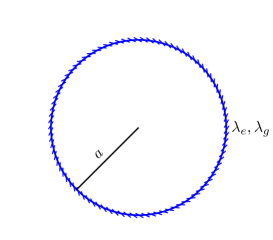
In this case, the magnetic scalar Green’s function is

$$g^{H}_{l}(r,r^{\prime};i\zeta)=\begin{cases}\frac{2}{\pi}\zeta\left[\text{i}_{l}(\zeta r_{<})\text{k}_{l}(\zeta r_{>})+\sigma^{\text{scatt}}_{l,<>}\,\text{i}_{l}(\zeta r)\text{i}_{l}(\zeta r^{\prime})\right],\quad&r,r^{\prime}<a,\\[8.53581pt] \frac{2}{\pi}\zeta\left[\text{i}_{l}(\zeta r_{<})\text{k}_{l}(\zeta r_{>})+\sigma^{\text{scatt}}_{l,><}\,\text{k}_{l}(\zeta r)\text{k}_{l}(\zeta r^{\prime})\right],&a<r,r^{\prime},\\[8.53581pt] \frac{2}{\pi}\zeta\,\sigma^{\text{abs}}_{l,><}\,\text{i}_{l}(\zeta r)\text{k}_{l}(\zeta r^{\prime}),&r<a<r^{\prime},\\[8.53581pt] \frac{2}{\pi}\zeta\,\sigma^{\text{abs}}_{l,<>}\,\text{k}_{l}(\zeta r)\text{i}_{l}(\zeta r^{\prime}),&r^{\prime}<a<r,\end{cases}$$ (33)

where the scattering coefficient $\sigma^{\text{scatt}}$ and absorption coefficients $\sigma^{\text{abs}}$ are

$\displaystyle\sigma^{\text{scatt}}_{l,<>}$ $\displaystyle=$ $\displaystyle-\frac{\left[\zeta\lambda^{\perp}_{e}\,\bar{\text{k}}\bar{\text{k}}-\zeta\lambda^{\perp}_{g}\,\text{k}\text{k}\right]}{\left[(1+\zeta^{2}\lambda^{\perp}_{e}\lambda^{\perp}_{g}/4)(\text{i}\bar{\text{k}}-\bar{\text{i}}\text{k})+\zeta\lambda^{\perp}_{e}\,\bar{\text{i}}\bar{\text{k}}-\zeta\lambda^{\perp}_{g}\,\text{i}\text{k}\right]}\xrightarrow[\lambda^{\perp}_{g}\to\infty]{\lambda^{\perp}_{e}\to\infty}0,$ (34a)
$\displaystyle\sigma^{\text{scatt}}_{l,><}$ $\displaystyle=$ $\displaystyle-\frac{\left[\zeta\lambda^{\perp}_{e}\,\bar{\text{i}}\bar{\text{i}}-\zeta\lambda^{\perp}_{g}\,\text{i}\text{i}\right]}{\left[(1+\zeta^{2}\lambda^{\perp}_{e}\lambda^{\perp}_{g}/4)(\text{i}\bar{\text{k}}-\bar{\text{i}}\text{k})+\zeta\lambda^{\perp}_{e}\,\bar{\text{i}}\bar{\text{k}}-\zeta\lambda^{\perp}_{g}\,\text{i}\text{k}\right]}\xrightarrow[\lambda^{\perp}_{g}\to\infty]{\lambda^{\perp}_{e}\to\infty}0,$ (34b)
$\displaystyle\sigma^{\text{abs}}_{l,><}=\sigma^{\text{abs}}_{l,<>}$ $\displaystyle=$ $\displaystyle\frac{(1+\zeta^{2}\lambda^{\perp}_{e}\lambda^{\perp}_{g}/4)(\text{i}\bar{\text{k}}-\bar{\text{i}}\text{k})}{\left[(1+\zeta^{2}\lambda^{\perp}_{e}\lambda^{\perp}_{g}/4)(\text{i}\bar{\text{k}}-\bar{\text{i}}\text{k})+\zeta\lambda^{\perp}_{e}\,\bar{\text{i}}\bar{\text{k}}-\zeta\lambda^{\perp}_{g}\,\text{i}\text{k}\right]}\xrightarrow[\lambda^{\perp}_{g}\to\infty]{\lambda^{\perp}_{e}\to\infty}-1,$ (34c)

where we have suppressed the argument and subscript to save typographical space. We use the modified spherical Bessel functions $\text{i}_{l}(t)$ and $\text{k}_{l}(t)$Ā NIS (2010) that are related to the modified Bessel functions as

$\displaystyle\text{i}_{l}(t)$ $\displaystyle=$ $\displaystyle\sqrt{\frac{\pi}{2t}}I_{l+\frac{1}{2}}(t),$ (35a)
$\displaystyle\text{k}_{l}(t)$ $\displaystyle=$ $\displaystyle\sqrt{\frac{\pi}{2t}}K_{l+\frac{1}{2}}(t).$ (35b)

In particular $\text{i}_{l}(t)=\text{i}^{(1)}_{l}(t)$, which is the modified spherical Bessel function of the first kind, and together with $\text{k}_{l}(t)$ are a satisfactory pair of solutions in the right half of the complex plane. We have also used bars to define the following operations on the modified spherical Bessel functions

$\displaystyle\bar{\text{i}}_{l}(t)$ $\displaystyle=$ $\displaystyle\bigg{(}\frac{1}{t}+\frac{\partial}{\partial t}\bigg{)}\text{i}_{l}(t),$ (36)
$\displaystyle\bar{\text{k}}_{l}(t)$ $\displaystyle=$ $\displaystyle\bigg{(}\frac{1}{t}+\frac{\partial}{\partial t}\bigg{)}\text{k}_{l}(t).$ (37)

Solutions for the electric Green’s function can be obtained from the magnetic Green’s function by replacing ${\bm{\varepsilon}}\leftrightarrow{\bm{\mu}}$ and $H\to E$.

We show the values of coefficients corresponding to a perfectly conducting electric and magnetic spherical shell in the rightmost listing in Eq. (34). Notice that the spherical shell becomes completely transparent in this extreme limit, and the total transmission is accompanied by a phase change of $\pi$.

It is crucial to emphasize the fact that even though we explicitly considered materials with $\lambda^{||}_{e}$ and $\lambda^{||}_{g}$ in Eqs.Ā (17), the solutions to the Green’s functions of Eq. (33) are independent of $\lambda^{||}_{e}$ and $\lambda^{||}_{g}$ because the boundary conditions in (32) do not depend on the parallel components of the coupling. The Green’s functions of Eqs. (33) determine the fields unambiguously everywhere except on the $\delta$-function plate, where we use an averaging prescription. The implication is that there are no observable consequences of $\lambda^{||}_{e}$ and $\lambda^{||}_{g}$.

V Casimir interaction energy between two concentric electric $\delta$-function spheres

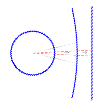
As a check for the formalism developed for a $\delta$-function sphere, we first calculate the Casimir interaction energy between two concentric electric $\delta$-function spheres as shown in Fig.Ā 3, where $\lambda_{g}=0$. We set $\lambda^{||}=0$ to satisfy the constraint given in Eq.Ā (24). In the asymptotic flat plate limit, i.e. small angle and large radius (See Fig.Ā 4), the interaction energy between the concentric $\delta$-function spheres should reproduce the interaction energy between two $\delta$-function plates. This limit coincides with the PFA for the spherical surfaces.

Refer to caption
Figure 3: Concentric $\delta$-function spheres with purely electric material properties.

The Casimir interaction energy between two concentric $\delta$-function spheres is

$$E_{12}=\frac{1}{2}\int_{-\infty}^{\infty}\frac{d\zeta}{2\pi}\sum_{l=1}^{\infty}\sum_{m=-l}^{l}{\operatorname{Tr}}\,\ln\left(\bf 1-{\bf K}\right),$$ (38)

where the notation $\operatorname{Tr}$ implies trace on both space coordinates (TrssubscriptTrš‘ \operatorname{Tr}_{s}) and matrix coordinates ($\operatorname{tr}$). The kernel ${\bf K}$ is

$${\bf K}(r,r^{\prime})={\bm{\gamma}}_{1}(r,r^{\prime})\cdot{\bm{\lambda}}_{e1}^{\perp}(r^{\prime})\delta(r^{\prime}-a_{1})\cdot{\bm{\gamma}}_{2}(r^{\prime},r)\cdot{\bm{\lambda}}_{e2}^{\perp}(r)\delta(r-a_{2}).$$ (39)

The interaction energy between two non-overlapping objects is always finite, hence we have dropped the cut-off parameters. Further, we can decompose Eq.Ā (38) into the TE and TM parts using the identity $\operatorname{tr}\,\ln{\bf K}=\ln\,\text{det}\,{\bf K}$

$${E}_{12}=\frac{1}{2}\int_{-\infty}^{\infty}\frac{d\zeta}{2\pi}\sum_{l}(2l+1)\int d^{3}x\left[\ln\left(1-K^{E}\right)+\operatorname{tr}\ln\left(\bf 1-{\bf K}^{H}\right)\right],$$ (40)

where $\text{K}^{E}$ corresponds to the 22 component of the kernel, which depends on the 22 component of Green’s dyadic given in (28), and ${\bf K}^{H}$ is rest of the matrix. The sum on $m$ is trivial as the magnetic Green’s function in Eq. (33) and the corresponding electric Green’s function are independent of $m$. One can verify that $\text{det}\,{\bf K}^{H}=0$, which implies that

$$\operatorname{Tr}\,\ln\left(1-{\bf K}^{H}\right)=\ln\left(1-\operatorname{Tr}\,{\bf K}^{H}\right).$$ (41)

The coefficients in Eq.Ā (34) for this case take the form

$\displaystyle\sigma^{\text{scatt}}_{l,<>}$ $\displaystyle=$ $\displaystyle-\frac{\zeta\lambda^{\perp}_{e}\,\bar{\text{k}}\bar{\text{k}}}{\left[(\text{i}\bar{\text{k}}-\bar{\text{i}}\text{k})+\zeta\lambda^{\perp}_{e}\,\bar{\text{i}}\bar{\text{k}}\right]}\xrightarrow{\lambda^{\perp}_{e}\to\infty}-\frac{\bar{\text{k}}}{\bar{\text{i}}},$ (42a)
$\displaystyle\sigma^{\text{scatt}}_{l,><}$ $\displaystyle=$ $\displaystyle-\frac{\zeta\lambda^{\perp}_{e}\,\bar{\text{i}}\bar{\text{i}}}{\left[(\text{i}\bar{\text{k}}-\bar{\text{i}}\text{k})+\zeta\lambda^{\perp}_{e}\,\bar{\text{i}}\bar{\text{k}}\right]}\xrightarrow{\lambda^{\perp}_{e}\to\infty}-\frac{\bar{\text{i}}}{\bar{\text{k}}},$ (42b)
$\displaystyle\sigma^{\text{abs}}_{l,><}=\sigma^{\text{abs}}_{l,<>}$ $\displaystyle=$ $\displaystyle\frac{(\text{i}\bar{\text{k}}-\bar{\text{i}}\text{k})}{\left[(\text{i}\bar{\text{k}}-\bar{\text{i}}\text{k})+\zeta\lambda^{\perp}_{e}\,\bar{\text{i}}\bar{\text{k}}\right]}\xrightarrow{\lambda^{\perp}_{e}\to\infty}0,$ (42c)

where the rightmost values are given for a perfectly conducting spherical shell. The TE part of the interaction energy between concentric $\delta$-function spheres is

$$E^{\mathrm{TE}}_{12}=\frac{1}{2}\int_{-\infty}^{\infty}\frac{d\zeta}{2\pi}\sum_{l}(2l+1)\ln\left[1-\frac{\zeta\lambda_{e1}^{\perp}}{\frac{\pi}{2(\zeta a_{1})^{2}}+\zeta\lambda_{e1}^{\perp}{\text{i}}_{l}(\zeta a_{1}){\text{k}}_{l}(\zeta a_{1})}\frac{\zeta\lambda_{e2}^{\perp}}{\frac{\pi}{2(\zeta a_{2})^{2}}+\zeta\lambda_{e2}^{\perp}{\text{i}}_{l}(\zeta a_{2}){\text{k}}_{l}(\zeta a_{2})}{\text{i}}_{l}^{2}(\zeta a_{1}){\text{k}}_{l}^{2}(\zeta a_{2})\right]$$ (43)

and the TM part of the interaction energy is

$$E^{\mathrm{TM}}_{12}=\frac{1}{2}\int_{-\infty}^{\infty}\frac{d\zeta}{2\pi}\sum_{l}(2l+1)\ln\left[1-\frac{\zeta\lambda_{e1}^{\perp}}{\frac{\pi}{2(\zeta a_{1})^{2}}-\zeta\lambda_{e1}^{\perp}{\bar{\text{i}}}_{l}(\zeta a_{1}){\bar{\text{k}}}_{l}(\zeta a_{1})}\frac{\zeta\lambda_{e2}^{\perp}}{\frac{\pi}{2(\zeta a_{2})^{2}}-\zeta\lambda_{e2}^{\perp}{\bar{\text{i}}}_{l}(\zeta a_{2}){\bar{\text{k}}}_{l}(\zeta a_{2})}{\bar{\text{i}}}_{l}^{2}(\zeta a_{1}){\bar{\text{k}}}_{l}^{2}(\zeta a_{2})\right].$$ (44)

In the asymptotic flat plate limit, which is equivalent to taking the uniform asymptotic expansion of the Bessel functions for $l\to\infty$, and keeping the distance between two spheres $a$ constant, we obtain the TE and TM mode interaction energies per unit area $\cal{E}$ for two parallel $\delta$-function plates:

Refer to caption
Figure 4: Flat plate limit: For a very large radius and small angle approximation a spherical surface is locally flat.
$\displaystyle{\cal E}^{\mathrm{TE}}_{12}$ $\displaystyle=$ $\displaystyle\frac{1}{2}\int_{-\infty}^{\infty}\frac{d\zeta}{2\pi}\int_{-\infty}^{\infty}\frac{d^{2}k}{(2\pi)^{2}}\ln\left(1-\frac{\lambda_{e1}^{\perp}}{\lambda_{e1}^{\perp}+\frac{2\kappa}{\zeta^{2}}}\frac{\lambda_{e2}^{\perp}}{\lambda_{e2}^{\perp}+\frac{2\kappa}{\zeta^{2}}}e^{-2\kappa a}\right),$ (45a)
$\displaystyle{\cal E}^{\mathrm{TM}}_{12}$ $\displaystyle=$ $\displaystyle\frac{1}{2}\int_{-\infty}^{\infty}\frac{d\zeta}{2\pi}\int_{-\infty}^{\infty}\frac{d^{2}k}{(2\pi)^{2}}\ln\left(1-\frac{\lambda_{e1}^{\perp}}{\lambda_{e1}^{\perp}+\frac{2}{\kappa}}\frac{\lambda_{e2}^{\perp}}{\lambda_{e2}^{\perp}+\frac{2}{\kappa}}e^{-2\kappa a}\right),$ (45b)

which gives the correct perfect conductor limit.

It is worth discussing the implication of the choice $\lambda^{||}=0$ here. We had pointed out in Eq.Ā (24) that a $\delta$-function boundary imposes constraints, $\lambda_{e}^{||}E^{(r)}(a)=0$ and $\lambda_{g}^{||}H^{(r)}(a)=0$. Additionally, the boundary conditions on the fields given by Eq.Ā (23) are independent of $\lambda^{||}$, thus the reflection coefficients appearing in Green’s function are independent of $\lambda^{||}$. These observations suggested a necessarily anisotropic nature of the $\delta$-function material with $\lambda$. Based on the above observations, we calculated the Casimir interaction energies using the multiple scattering method in Eq.Ā (38) for the TE and TM mode for $\bm{\lambda}=\left(\lambda^{\perp},\lambda^{\perp},0\right)$ requiring $\lambda^{||}=0$, which for the parallel plate case are given in Eq. (45). Let us explore the case when we ignore this constraint and keep $\lambda^{||}\neq 0$ in $\bm{\lambda}=\left(\lambda^{\perp},\lambda^{\perp},\lambda^{||}\right)$. In this case, the interaction energy of the TM mode would become

$$\frac{1}{2}\int_{-\infty}^{\infty}\frac{d\zeta}{2\pi}\int_{-\infty}^{\infty}\frac{d^{2}k}{(2\pi)^{2}}\ln\left[1-\left(\frac{\lambda_{e1}^{\perp}}{\lambda_{e1}^{\perp}+\frac{2}{\kappa}}+k^{2}_{\perp}\frac{\lambda_{e1}^{||}}{2\kappa}\right)\left(\frac{\lambda_{e2}^{\perp}}{\lambda_{e2}^{\perp}+\frac{2}{\kappa}}+k^{2}_{\perp}\frac{\lambda_{e2}^{||}}{2\kappa}\right)e^{-2\kappa a}\right].$$

This would suggest the identification of a TM ā€œreflection coefficientā€ of a single $\delta$-function plate of the form

$$\frac{\lambda_{ei}^{\perp}}{\lambda_{ei}^{\perp}+\frac{2}{\kappa}}+k^{2}_{\perp}\frac{\lambda_{ei}^{||}}{2\kappa},$$ (46)

which is inconsistent with the reflection coefficients found in the solutions of Green’s functions using the boundary conditions as explained below. First we note that the second term is the added contribution due to the inclusion of the nonzero $\lambda^{||}$ in the Casimir interaction energy calculation. But this is not satisfactory because the reflection coefficient in Eq.Ā (46) doesn’t have a finite limit in $\lambda^{||}\to\infty$. At best, it suggests a weak behavior of $\lambda^{||}$. In other words, a $\delta$-function material can only have high conductivity in the surface of the material, which seems to be a physically viable option for an infinitesimally thin material. Secondly and more importantly, in Ref.Ā ParasharĀ etĀ al. (2012); *Shajesh:2017axs we show by a direct calculation of Green’s function for $\delta$-function plates that the reflection coefficients do not depend on the $\lambda^{||}$, which is a consequence of the fact that the boundary conditions are not contingent on the $\lambda^{||}$. Thus, the appearance of $\lambda^{||}$ in (46) belies the adage that one can determine the Casimir (Lifshitz) interaction energy once the reflection coefficients are known. These observations strongly advocate for $\lambda^{||}=0$ as the consistent choice.

VI Self energy of a $\delta$-function sphere

We are particularly interested in analyzing the self-energy of a $\delta$-function sphere, which in general has divergent parts. We will use the point-splitting regulator for evaluating the self-energy. For a nonzero value of the point-splitting regulator $\bm{\delta}$ (where $\bm{\delta}$ has both temporal and spatial point-splitting components) the energy remains finite but it diverges in the limit $\bm{\delta}\to 0$. Using Maxwell’s equations and the definition of Green’s dyadic in Eq.Ā  (26), we can rewrite the bulk subtracted energy given in Eq.Ā (14) for a dispersive magneto-electric material as

$$E-E_{0}=\frac{1}{2}\int_{-\infty}^{\infty}\frac{d\zeta}{2\pi}\int d^{3}x\,\frac{e^{i\zeta\tau}-1}{i\zeta\tau}\operatorname{tr}\Big{[}2{\bm{\varepsilon}}\cdot{\bm{\Gamma}}+\zeta\frac{d\bm{\varepsilon}}{d\zeta}\cdot{\bm{\Gamma}}-{\bm{\mu}}^{-1}\cdot\frac{d\bm{\mu}}{d\zeta}\cdot({\bm{\Phi}}\times\overleftarrow{\bm{\nabla}^{\prime}})-2{\bm{\Gamma}}_{0}\Big{]}\bigg{|}_{{\bf x}^{\prime}={\bf x}+{\bm{\delta}}}.$$ (47)

Using the expansion of Green’s dyadics in vector spherical harmonics and choosing the point-splitting in both temporal and spatial directions we can express the self-energy in terms of reduced Green’s dyadic

$$E-E_{0}=\frac{1}{2}\int_{-\infty}^{\infty}\frac{d\zeta}{2\pi}\frac{e^{i\zeta\tau}-1}{i\zeta\tau}\sum_{l}(2l+1)P_{l}(\cos\delta)\,I,$$ (48a)
where
$$I=\int_{0}^{\infty}r^{2}dr\,\operatorname{tr}\Big{[}2{\bm{\varepsilon}}\cdot{\bm{\gamma}}+\zeta\frac{d\bm{\varepsilon}}{d\zeta}\cdot{\bm{\gamma}}-{\bm{\mu}}^{-1}\cdot\frac{d\bm{\mu}}{d\zeta}\cdot({\bm{\phi}}\times\overleftarrow{\bm{\nabla}^{\prime}})-2{\bm{\gamma}}_{0}\Big{]}\Big{|}_{r^{\prime}=r}.$$ (48b)

In the following, we shall continue with the choice of purely electric $\delta$-function materials, i.e. $\lambda_{g}=0$. We also need to choose a particular model to define the frequency-dependent coupling constant in order to account for the dispersion, which is relevant for the energy calculated from Eq.Ā (47). A sort of plasma model, $\lambda^{\perp}_{e}=\zeta_{p}/\zeta^{2}$, is a straightforward choice, where $\zeta_{p}$ is an effective plasma frequency. (This is identical to Barton’s hydrodynamical model, where the parameter $\zeta_{p}$ corresponds to the characteristic wavenumber Barton (2005).)

VI.1 Self energy of an electric $\delta$-function plate

We first apply the energy expression in Eq.Ā (47) to calculate the self-energy of a purely electric $\delta$-function plate ($\lambda^{\perp}_{g}=0$ and $\lambda^{\perp}_{e}=\zeta_{p}/\zeta^{2}$). Keeping only the spatial cut-off $\bm{\delta}_{\perp}$ we obtain the energy per unit area,

$${\cal E}-{\cal E}_{0}=\frac{1}{2}\int_{-\infty}^{\infty}\frac{d\zeta}{2\pi}\int\frac{d^{2}k}{(2\pi)^{2}}e^{i{\bf k}\cdot{\bm{\delta}}_{\perp}}\int_{-\infty}^{\infty}dz\,\operatorname{tr}\Big{[}2{\bm{\varepsilon}}\cdot{\bm{\gamma}}+\zeta\frac{d\bm{\varepsilon}}{d\zeta}\cdot{\bm{\gamma}}-2{\bm{\gamma}}_{0}\Big{]}\Big{|}_{z^{\prime}=z}.$$ (49)

It is evident that the second term in the energy expression (47) does not vanish in this case. In fact, this term cancels the $\delta$-function piece coming from the first term. The self-energy for the TE mode is

$$({\cal E}-{\cal E}_{0})^{\mathrm{TE}}=\frac{1}{8\pi^{2}}\int_{0}^{\infty}d\kappa\kappa^{2}\int_{-1}^{1}d(\cos\beta)\cos^{2}\beta\int_{0}^{2\pi}d\alpha\,e^{i\kappa{\delta}_{\perp}\sin\beta}\frac{\zeta_{p}}{\zeta_{p}+2\kappa},$$ (50)

where $\kappa=\sqrt{k^{2}+\zeta^{2}}$. For an arbitrary coupling the TE energy per unit area is

$\displaystyle({\cal E}-{\cal E}_{0})^{\mathrm{TE}}$ $\displaystyle=$ $\displaystyle\frac{1}{8\pi^{2}\delta_{\perp}^{3}}\left\{\pi-\sin\frac{\zeta_{p}\,\delta_{\perp}}{2}\left[2\mbox{Ci}\left(\frac{\zeta_{p}\,\delta_{\perp}}{2}\right)+\frac{\zeta_{p}\,\delta_{\perp}}{2}\left(\pi-2\mbox{Si}\left(\frac{\zeta_{p}\,\delta_{\perp}}{2}\right)\right)\right]\right.$ (51)
$\displaystyle\hskip 45.5244pt\left.+\cos\frac{\zeta_{p}\,\delta_{\perp}}{2}\left[-\pi+2\frac{\zeta_{p}\,\delta_{\perp}}{2}\mbox{Ci}\left(\frac{\zeta_{p}\,\delta_{\perp}}{2}\right)+2\mbox{Si}\left(\frac{\zeta_{p}\,\delta_{\perp}}{2}\right)\right]\right\},$

where $\mbox{Ci}(x)$ and $\mbox{Si}(x)$ are the standard cosine integral and sine integral functions, respectively. For the finite coupling, $\zeta_{p}$, and in the $\delta_{\perp}\to 0$ limit we obtain the result identical to the divergence structure obtained in the analysis of the self-energy of a $\delta$-function plate interacting with a scalar fieldĀ MiltonĀ etĀ al. (2014),

$$({\cal E}-{\cal E}_{0})^{\mathrm{TE}}_{\delta_{\perp}\to 0}=\frac{\zeta_{p}}{8\pi^{2}\delta_{\perp}^{2}}\left\{1-\frac{\pi}{4}\left(\frac{\zeta_{p}\,\delta_{\perp}}{2}\right)+\frac{1}{3}\left(\frac{\zeta_{p}\,\delta_{\perp}}{2}\right)^{2}\left[\frac{4}{3}-\gamma-\ln\left(\frac{\zeta_{p}\,\delta_{\perp}}{2}\right)\right]\right\}+{\cal O}(\delta_{\perp}).$$ (52)

In the strong coupling limit $\zeta_{p}\to\infty$, keeping $\delta_{\perp}$ finite, we recover the inverse cubic divergence,

$$({\cal E}-{\cal E}_{0})^{\mathrm{TE}}_{\lambda\to\infty}=\frac{1}{8\pi\delta_{\perp}^{3}}.$$ (53)

The TM mode energy is

$$({\cal E}-{\cal E}_{0})^{\mathrm{TM}}=\frac{1}{8\pi^{2}}\int_{0}^{\infty}d\kappa\kappa^{2}\int_{-1}^{1}d(\cos\beta)(1+\sin^{2}\beta)J_{0}(\kappa\delta_{\perp}\sin\beta)\frac{\zeta_{p}}{\zeta_{p}+2\kappa\cos^{2}\beta}.$$ (54)

In the strong coupling limit $\zeta_{p}\to\infty$, we obtain an inverse third power of point-splitting parameter as in (53) with opposite sign. Thus in the strong coupling the total energy per unit area show no divergence.

To obtain the finite or weak coupling divergence structure for the TM, we first write the integrand as

$$({\cal E}-{\cal E}_{0})^{\mathrm{TM}}=\frac{1}{8\pi^{2}}\sum_{q=0}^{\infty}(-1)^{q}\left(\frac{\lambda}{2}\right)^{q+1}\int_{-1}^{1}d(\cos\beta)\frac{(1+\sin^{2}\beta)}{(\cos\beta)^{(2q+2)}}\int_{0}^{\infty}d\kappa\,\kappa^{(1-q)}J_{0}(\kappa\delta_{\perp}\sin\beta).$$ (55)

We now carry out the $\kappa$ and $\cos\beta$ integrations for a fixed $k$,

$$({\cal E}-{\cal E}_{0})^{\mathrm{TM}}=\frac{1}{8\pi^{2}}\sum_{q=0}^{\infty}(-1)^{q}\left(\frac{\lambda}{2}\right)^{q+1}\frac{1}{2^{(1+q)}\pi}q\,\delta^{-2+q}\cos\frac{q\pi}{2}\,\Gamma\left(-\frac{1}{2}-q\right)\Gamma\left(-\frac{q}{2}\right)\Gamma\left(\frac{q}{2}\right),\qquad\frac{1}{2}<q<2.$$ (56)

We are only interested in looking at the divergence behavior of the TM self-energy of the $\delta$-function plate in the limit $\delta_{\perp}\to 0$, so we shall evaluate the above expression for $q=0,1,2$. The above expression has finite limit for $q=0,1$ and has a pole at $q=2$, which presumably could be removed by introducing a small photon mass. Keeping all the terms together we find,

$$({\cal E}-{\cal E}_{0})^{\mathrm{TM}}_{\delta_{\perp}\to 0}=\frac{\zeta_{p}}{8\pi^{2}\delta_{\perp}^{2}}\left\{1+\frac{1}{15}\left(\frac{\zeta_{p}\,\delta_{\perp}}{2}\right)^{2}\left[\frac{1}{q-2}+\ln\left(\frac{\zeta_{p}\,\delta_{\perp}}{2}\right)-\frac{\gamma}{2}-\ln 2-\psi\left(-\frac{5}{2}\right)+\frac{1}{2}\psi\left(\frac{3}{2}\right)\right]\right\}+{\cal O}(\delta_{\perp}).$$ (57)

Notice that divergences in Eqs. (52) and (57) do not cancel between the TE and TM mode. We shall see a similar behavior for the finite coupling case of the $\delta$-function sphere.

VI.2 Self energy of a electric $\delta$-function sphere

Next we consider the purely electric $\delta$-function sphere. With the choice of the plasma model described above, the TE and TM Green’s functions obtained here coincide with those discussed in Refs.Ā Milton (2004a, b, 2011, 2003) with the identification of $\lambda^{\rm TE}=a^{2}\zeta_{p}=-x^{2}\lambda^{\rm TM}$, and the redefinition of spherical Bessel function in terms of modified Riccati-Bessel function as sl=x​ilsubscriptš‘ š‘™š‘„subscriptiš‘™s_{l}=x\,{\text{i}}_{l} and $e_{l}=\frac{2}{\pi}x\,{\text{k}}_{l}$. Thus the results found there, with errors corrected in Ref.Ā Milton (2011), for the energy and the stress on the sphere, follow with the above coupling constant identification.

The integral $I$ defined in Eq.Ā (48b) in this case becomes

$$I=\int_{0}^{\infty}r^{2}dr\left[2{\bm{\gamma}}+\frac{2}{\zeta^{2}}{\bm{\zeta}}_{p}\cdot{\bm{\gamma}}\delta(r-a)-\frac{2}{\zeta^{2}}\zeta_{p}\cdot{\bm{\gamma}}\delta(r-a)-2{\bm{\gamma}}_{0}\right]=\int_{0}^{\infty}r^{2}dr2\left({\bm{\gamma}}-{\bm{\gamma}}_{0}\right),$$ (58)

where the $\delta$-function terms coming from the first and the second terms cancel, similar to the $\delta$-function plate case. If we fail to take the dispersion term in account, then we would get additional contributions from the remaining $\delta$-function term.

The integrals for the TE and TM mode are

$\displaystyle I^{\mathrm{TE}}$ $\displaystyle=$ $\displaystyle 2\int_{0}^{\infty}r^{2}dr\zeta^{2}\frac{2\zeta}{\pi}\left[\theta(a-r)\sigma^{\text{scatt(E)}}_{l,><}{\text{i}}^{2}_{l}(\zeta r)+\theta(r-a)\sigma^{\text{scatt(E)}}_{l,<>}{\text{k}}^{2}_{l}(\zeta r)\right],$
$\displaystyle I^{\mathrm{TM}}$ $\displaystyle=$ $\displaystyle 2\int_{0}^{\infty}r^{2}dr\frac{2\zeta}{\pi}\left[\theta(a-r)\sigma^{\text{scatt(H)}}_{l,><}\left(\zeta^{2}{\bar{\text{i}}}^{2}_{l}(\zeta r)+\frac{l(l+1)}{r^{2}}{\text{i}}^{2}_{l}(\zeta r)\right)+\theta(r-a)\sigma^{\text{scatt(H)}}_{l,<>}\left(\zeta^{2}{\bar{\text{i}}}^{2}_{l}(\zeta r)+\frac{l(l+1)}{r^{2}}{\text{k}}^{2}_{l}(\zeta r)\right)\right].$

The above expressions are valid for the general case where both electric and magnetic coupling can be present. From Eqs.Ā (34), it is evident that the integrand $I$ will vanish identically. This implies that the self-energy of a $\delta$-function shell that is both perfectly electrically conducting and a perfectly magnetically conducting is zero including the divergences! Such a shell does not have any optical interaction up to a phase.

Using the identities

$\displaystyle\int_{0}^{\infty}dx\,x^{2}\,{\text{i}}_{l}^{2}(x)$ $\displaystyle=$ $\displaystyle\frac{x}{2}\left[(x^{2}+l(l+1)){\text{i}}^{2}-x\,{\text{i}}_{l}{\text{i}}_{l}^{\prime}-x^{2}\,{\text{i}}_{l}^{\prime 2}\right],$ (60a)
$\displaystyle\int_{0}^{\infty}dx\,x^{2}\,{\text{k}}_{l}^{2}(x)$ $\displaystyle=$ $\displaystyle-\frac{x}{2}\left[(x^{2}+l(l+1)){\text{k}}^{2}-x\,{\text{k}}_{l}{\text{k}}_{l}^{\prime}-x^{2}\,{\text{k}}_{l}^{\prime 2}\right],$ (60b)

and the Wronskian $W[{\text{i}}_{l}(x),{\text{k}}_{l}(x)]=-\frac{\pi}{2x^{2}}$, and keeping both temporal and spatial point-splitting we obtain the energy for the TE and TM mode as

$\displaystyle E^{\mathrm{TE}}$ $\displaystyle=$ $\displaystyle-\frac{1}{2}\int_{-\infty}^{\infty}\frac{d\zeta}{2\pi}\frac{e^{i\zeta\tau}-1}{i\zeta\tau}\sum_{l=1}^{\infty}(2l+1)P_{l}(\cos\delta)\zeta\frac{d}{d\zeta}\ln\left[1+\zeta_{p}a\frac{2}{\pi}x\,{\text{i}_{l}(x)}{\text{k}_{l}(x)}\right],$ (61a)
$\displaystyle E^{\mathrm{TM}}$ $\displaystyle=$ $\displaystyle-\frac{1}{2}\int_{-\infty}^{\infty}\frac{d\zeta}{2\pi}\frac{e^{i\zeta\tau}-1}{i\zeta\tau}\sum_{l=1}^{\infty}(2l+1)P_{l}(\cos\delta)\zeta\frac{d}{d\zeta}\ln\left[-1+\zeta_{p}a\frac{2}{\pi}x\,{\bar{\text{i}}_{l}(x)}_{l}{\bar{\text{k}}_{l}(x)}_{l}\right],$ (61b)

where $x=|\zeta|a$ for a sphere of radius $a$.

Thus the total self-energy of an electric $\delta$-function sphere is

E=āˆ’12ā€‹āˆ«āˆ’āˆžāˆžd​ζ2​π​eiā€‹Ī¶ā€‹Ļ„āˆ’1iā€‹Ī¶ā€‹Ļ„ā€‹āˆ‘l=1āˆž(2​l+1)​Pl​(cos⁔Γ)​ζ​dd​ζ​ln⁔[1+ζp​a​el​(x)​sl​(x)x]​[1āˆ’Ī¶p​a​el′​(x)​sl′​(x)x],šø12superscriptsubscriptš‘‘šœ2šœ‹superscriptš‘’š‘–šœšœ1š‘–šœšœsuperscriptsubscriptš‘™12š‘™1subscriptš‘ƒš‘™š›æšœš‘‘š‘‘šœ1subscriptšœš‘š‘Žsubscriptš‘’š‘™š‘„subscriptš‘ š‘™š‘„š‘„delimited-[]1subscriptšœš‘š‘Žsuperscriptsubscriptš‘’š‘™ā€²š‘„superscriptsubscriptš‘ š‘™ā€²š‘„š‘„E=-\frac{1}{2}\int_{-\infty}^{\infty}\frac{d\zeta}{2\pi}\frac{e^{i\zeta\tau}-1}{i\zeta\tau}\sum_{l=1}^{\infty}(2l+1)P_{l}(\cos\delta)\zeta\frac{d}{d\zeta}\ln\left[1+\zeta_{p}a\frac{e_{l}(x)s_{l}(x)}{x}\right]\left[1-\zeta_{p}a\frac{e_{l}^{\prime}(x)s_{l}^{\prime}(x)}{x}\right], (62)

where we have used the prevalent modified Riccati-Bessel functions. In Ref.Ā Milton (2004b, 2011), we tried to make sense of this expression without serious regulation. Now, everything will be well-defined, and we shall study carefully the cutoff dependences.

VI.2.1 Strong couping

In the perfect conducting limit $\zeta_{p}\to\infty$ (strong coupling) we recover the standard result, which is the well-studied Boyer problemĀ Boyer (1968); Davies (1972); BalianĀ andĀ Duplantier (1978); MiltonĀ etĀ al. (1978); LeseduarteĀ andĀ Romeo (1996); NesterenkoĀ andĀ Pirozhenko (1998).

$\displaystyle E-E_{0}$ $\displaystyle=$ āˆ’14ā€‹Ļ€ā€‹āˆ‘l=1āˆž(2​l+1)​Pl​(cos⁔Γ)ā€‹āˆ«āˆ’āˆžāˆžš‘‘Ī¶ā€‹eiā€‹Ī¶ā€‹Ļ„āˆ’1i​ζ​τ​ζ​dd​ζ​ln⁔el​sl​el′​sl′x214šœ‹superscriptsubscriptš‘™12š‘™1subscriptš‘ƒš‘™š›æsuperscriptsubscriptdifferential-dšœsuperscriptš‘’š‘–šœšœ1š‘–šœšœšœš‘‘š‘‘šœsubscriptš‘’š‘™subscriptš‘ š‘™superscriptsubscriptš‘’š‘™ā€²superscriptsubscriptš‘ š‘™ā€²superscriptš‘„2\displaystyle-\frac{1}{4\pi}\sum_{l=1}^{\infty}(2l+1)P_{l}(\cos\delta)\int_{-\infty}^{\infty}d\zeta\frac{e^{i\zeta\tau}-1}{i\zeta\tau}\zeta\frac{d}{d\zeta}\ln\frac{e_{l}s_{l}e_{l}^{\prime}s_{l}^{\prime}}{x^{2}}
$\displaystyle=$ āˆ’14ā€‹Ļ€ā€‹āˆ‘l=1āˆž(2​l+1)​Pl​(cos⁔Γ)ā€‹āˆ«āˆ’āˆžāˆžš‘‘Ī¶ā€‹eiā€‹Ī¶ā€‹Ļ„āˆ’1i​ζ​τ​ζ​[sl′sl+el′el+sl′′sl′+el′′elā€²āˆ’2x].14šœ‹superscriptsubscriptš‘™12š‘™1subscriptš‘ƒš‘™š›æsuperscriptsubscriptdifferential-dšœsuperscriptš‘’š‘–šœšœ1š‘–šœšœšœdelimited-[]superscriptsubscriptš‘ š‘™ā€²subscriptš‘ š‘™superscriptsubscriptš‘’š‘™ā€²subscriptš‘’š‘™superscriptsubscriptš‘ š‘™ā€²ā€²superscriptsubscriptš‘ š‘™ā€²superscriptsubscriptš‘’š‘™ā€²ā€²superscriptsubscriptš‘’š‘™ā€²2š‘„\displaystyle-\frac{1}{4\pi}\sum_{l=1}^{\infty}(2l+1)P_{l}(\cos\delta)\int_{-\infty}^{\infty}d\zeta\,\frac{e^{i\zeta\tau}-1}{i\zeta\tau}\zeta\left[\frac{s_{l}^{\prime}}{s_{l}}+\frac{e_{l}^{\prime}}{e_{l}}+\frac{s_{l}^{\prime\prime}}{s_{l}^{\prime}}+\frac{e_{l}^{\prime\prime}}{e_{l}^{\prime}}-\frac{2}{x}\right].

Here, we carefully extract the divergent terms, and obtain the familiar finite remainder. First, we note that the $\ln(1/x)$ term does not contribute, because

$$\int_{-\infty}^{\infty}\frac{d\zeta}{i\zeta\tau}\left(e^{i\zeta\tau}-1\right)=\frac{2}{\tau}\int_{-\infty}^{\infty}\frac{d\zeta}{\zeta}e^{i\zeta\tau/2}\sin\frac{\zeta\tau}{2}=\frac{\pi}{\tau},$$ (64)

which is a constant, independent of the size of the sphere, so the corresponding contribution to the energy is irrelevant.

To proceed, we use the uniform asymptotic expansions for the Bessel functions to find for large $\nu=l+1/2$,

ln⁔el​el′​sl​slā€²āˆ¼āˆ’ln⁔4āˆ’t64​ν2+t632​ν4​(4āˆ’54​t2+120​t4āˆ’71​t6)+O​(Ī½āˆ’6).similar-tosubscriptš‘’š‘™superscriptsubscriptš‘’š‘™ā€²subscriptš‘ š‘™superscriptsubscriptš‘ š‘™ā€²4superscriptš‘”64superscriptšœˆ2superscriptš‘”632superscriptšœˆ4454superscriptš‘”2120superscriptš‘”471superscriptš‘”6š‘‚superscriptšœˆ6\ln e_{l}e_{l}^{\prime}s_{l}s_{l}^{\prime}\sim-\ln 4-\frac{t^{6}}{4\nu^{2}}+\frac{t^{6}}{32\nu^{4}}(4-54t^{2}+120t^{4}-71t^{6})+O(\nu^{-6}). (65)

Here $x=|\zeta|a=\nu z$ and $t=(1+z^{2})^{-1/2}$. The order $\nu^{-2}$ term gives rise to a divergent contribution to the energy in the absence of a cutoff. With the above cutoff, that term yields the energy contribution

$$E^{(2)}=\frac{1}{8\pi a}\sum_{l=1}^{\infty}P_{l}(\cos\delta)\int_{-\infty}^{\infty}dz\frac{e^{i\nu z\tilde{\tau}}-1}{i\nu z\tilde{\tau}}z\frac{d}{dz}\frac{1}{(1+z^{2})^{3}},$$ (66)

with $\tilde{\tau}=\tau/a$. The $z$ integral is easily evaluated, leaving

$\displaystyle E^{(2)}$ $\displaystyle=$ $\displaystyle-\frac{1}{64a}\sum_{l=1}^{\infty}P_{l}(\cos\delta)e^{-\nu\tilde{\tau}}(3+3\nu\tilde{\tau}+\nu^{2}\tilde{\tau}^{2})$ (67)
$\displaystyle=$ $\displaystyle-\frac{1}{64a}\left(3-3\tilde{\tau}\frac{\partial}{\partial\tilde{\tau}}+\tilde{\tau}^{2}\frac{\partial^{2}}{\partial\tilde{\tau}^{2}}\right)\sum_{l=1}^{\infty}P_{l}(\cos\delta)e^{-\nu\tilde{\tau}}.$

In the limit of small $\tau$ and $\delta$, the sum on $l$ is evaluated, using the generating function for the Legendre polynomials,

$$\sum_{l=1}^{\infty}P_{l}(\cos\delta)e^{-\nu\tilde{\tau}}=-1+\frac{1}{\Delta},\quad\Delta=\sqrt{\delta^{2}+\tilde{\tau}^{2}}.$$ (68)

Thus the divergent term in strong coupling is

$$E^{(2)}=\frac{3}{64a}-\frac{1}{64a\Delta^{5}}(3\delta^{4}+8\delta^{2}\tilde{\tau}^{2}+8\tilde{\tau}^{4}).$$ (69)

Geometrically, the divergent term, as $\delta$ and $\tilde{\tau}$ tend to zero, corresponds to a surface integral of the curvature-squared divergence, which is uncanceled between the TE and TM modes, and between interior and exterior contributions. On the other hand, the finite part, which arises entirely from the omitted $l=0$ term in the sum, $3/(64a)$, is within 2% of the exact repulsive resultĀ MiltonĀ etĀ al. (1978).

This result seems rather surprising, since the conventional wisdom is that this divergence is not present for a perfectly conducting spherical shell of zero thicknessĀ Fulling (2003). Indeed, the $a_{2}$ heat kernel coefficient for this problem vanishes. To elucidate this conundrum, we note that the form of the temporal cutoff used here is a bit unconventional. What was actually used in the time-split regulated calculation in Ref.Ā MiltonĀ etĀ al. (1978) was simply $e^{i\nu z\tilde{\tau}}$ rather than $(e^{i\nu z\tilde{\tau}}-1)/i\nu z\tilde{\tau}$. We can verify that if the above calculation is repeated for the former regulator, we instead find

$$E^{(2)\prime}=\frac{3}{64a}-\frac{3}{64a}\frac{\delta^{2}}{\Delta^{7}}(\delta^{4}+4\delta^{2}\tilde{\tau}^{2}+8\tilde{\tau}^{4}).$$ (70)

Now, if the spatial cutoff is set to zero, $\delta=0$, the divergent term vanishes! This seems to be the content of the heat-kernel approach. And, in fact, with a purely spatial regulator,

$$E^{(2)}=\frac{3}{64a}\left(1-\frac{1}{\delta}\right).$$ (71)

This result was anticipated, for example, in Refs.Ā MiltonĀ etĀ al. (2013b, c) (see also Refs.Ā DowkerĀ andĀ Apps (1995); AppsĀ andĀ Dowker (1998); NesterenkoĀ etĀ al. (2003)) where it was found for a single curvature, the TE and TM integrated curvature squared divergent contributions are for an arc of angle $\alpha$

$$\mbox{TE}:\quad-\frac{1}{\pi}\frac{\alpha}{1024a\delta},\quad\mbox{TM}:\quad-\frac{1}{\pi}\frac{5\alpha}{1024a\delta},$$ (72)

so when $\alpha=2\pi$, the sum of these two multiplied by 4 (two curvatures, and inside and outside contributions) yields the divergence found in Eq.Ā (71), and further the ratio of the TE and TM contributions, 1/5, is indeed found here when the individual contributions are examined. (See Eq.Ā (73), below.)

Now to extract the finite part, we can follow the procedure given in Refs.Ā BenderĀ andĀ Milton (1994); Milton (1997b), and use the following asymptotic evaluations of the integrals, with $\tau=0$,

$\displaystyle Q_{l}^{\rm TM}$ $\displaystyle=$ ∫0āˆžš‘‘x​ln⁔(āˆ’2​el′​sl′)āˆ¼Ļ€ā€‹Ī½2āˆ’5​π128ā€‹Ī½āˆ’53​π32769​ν3āˆ’901​π2097152​ν5+…,similar-tosuperscriptsubscript0differential-dš‘„2superscriptsubscriptš‘’š‘™ā€²superscriptsubscriptš‘ š‘™ā€²šœ‹šœˆ25šœ‹128šœˆ53šœ‹32769superscriptšœˆ3901šœ‹2097152superscriptšœˆ5…\displaystyle\int_{0}^{\infty}dx\ln(-2e_{l}^{\prime}s_{l}^{\prime})\sim\frac{\pi\nu}{2}-\frac{5\pi}{128\nu}-\frac{53\pi}{32769\nu^{3}}-\frac{901\pi}{2097152\nu^{5}}+\dots, (73a)
$\displaystyle Q_{l}^{\rm TE}$ $\displaystyle=$ ∫0āˆžš‘‘x​ln⁔(2​el​sl)āˆ¼āˆ’Ļ€ā€‹Ī½2āˆ’Ļ€128​ν+35​π32769​ν3āˆ’565​π1048576​ν5+…,similar-tosuperscriptsubscript0differential-dš‘„2subscriptš‘’š‘™subscriptš‘ š‘™šœ‹šœˆ2šœ‹128šœˆ35šœ‹32769superscriptšœˆ3565šœ‹1048576superscriptšœˆ5…\displaystyle\int_{0}^{\infty}dx\ln(2e_{l}s_{l})\sim-\frac{\pi\nu}{2}-\frac{\pi}{128\nu}+\frac{35\pi}{32769\nu^{3}}-\frac{565\pi}{1048576\nu^{5}}+\dots, (73b)

so the total integral here is

$$Q_{l}=Q_{l}^{\rm TE}+Q_{l}^{\rm TM}\sim-\frac{3\pi}{64\nu}-\frac{9\pi}{16348\nu^{3}}-\frac{2031\pi}{2097152\nu^{5}}+\dots.$$ (74)

Thus with spatial regulation the energy has the form

$$E=\frac{1}{2\pi a}\sum_{l=0}^{\infty}(2l+1)P_{l}(\cos\delta)Q_{l}+\frac{\pi}{48a},$$ (75)

where it is convenient to start the sum at $l=0$, so we subtract off the value of that term. Putting in the first three terms of the asymptotic expansion gives us

$$E-\frac{\pi}{48a}\sim-\frac{3}{64a\delta}-\frac{1}{a}\left(\frac{9\pi^{2}}{32768}+\frac{677\pi^{4}}{4194304}\right)=-\frac{3}{64a\delta}-\frac{0.0184335}{a}.$$ (76)

To this we must add the remainder, obtained from Eq.Ā (75) by subtracting the first three asymptotic terms given in (74) from $Q_{l}$:

$$R=\frac{1}{\pi a}\sum_{l=0}^{\infty}\nu\left(Q_{l}+\frac{3\pi}{64\nu}+\frac{9\pi}{16384\nu^{3}}+\frac{2031\pi}{2097152\nu^{5}}\right).$$ (77)

The sum converges rapidly; going out to $l=2$ is sufficient to give $R=-0.000840$, giving us for the energy

$$E=-\frac{3}{64a\delta}+\frac{0.046176}{a},$$ (78)

where the finite part is the standard number for a perfectly conducting sphere. Note that the first approximation we had in Eq.Ā (69) is high by only 1.5%.

VI.2.2 Finite Coupling

We now return to the general expression (62), and start by analyzing the divergences occurring there as the cutoff parameters $\delta$ and $\tau$ approach zero. In doing so, we again use the uniform asymptotic expansion for the Bessel functions; we immediately encounter a difficulty in that the TM mode contributions yield a spurious infrared divergence, because of the $1/z$ behavior for small $z$. To cure this, we insert an infrared cutoff as well: We replace

$$\frac{1}{z^{2}t}=\frac{\sqrt{1+z^{2}}}{z^{2}}\to\frac{\sqrt{z^{2}+1}}{z^{2}+1}=t;$$ (79)

we could insert an arbitrary infrared cutoff parameter, but that introduces unnecessary complications, since in principle we will be adding back the same terms that we subtract. This way we can treat the TE and TM modes on the same footing.

The divergences occur in the asymptotic expansion of the logarithm in Eq.Ā (62), which we write as

ln⁔(1+ζp​ax​el​sl)​(1āˆ’Ī¶p​ax​el′​sl′)āˆ¼āˆ‘k=1āˆža(k)(2​ν)k,similar-to1subscriptšœš‘š‘Žš‘„subscriptš‘’š‘™subscriptš‘ š‘™1subscriptšœš‘š‘Žš‘„superscriptsubscriptš‘’š‘™ā€²superscriptsubscriptš‘ š‘™ā€²superscriptsubscriptš‘˜1superscriptš‘Žš‘˜superscript2šœˆš‘˜\ln\left(1+\frac{\zeta_{p}a}{x}e_{l}s_{l}\right)\left(1-\frac{\zeta_{p}a}{x}e_{l}^{\prime}s_{l}^{\prime}\right)\sim\sum_{k=1}^{\infty}\frac{a^{(k)}}{(2\nu)^{k}}, (80)

where a simple calculation gives

$\displaystyle a^{(1)}$ $\displaystyle=$ $\displaystyle 2\zeta_{p}at,$ (81a)
$\displaystyle a^{(2)}$ $\displaystyle=$ $\displaystyle-\zeta_{p}^{2}a^{2}t^{2},$ (81b)
$\displaystyle a^{(3)}$ $\displaystyle=$ $\displaystyle\frac{\zeta_{p}a}{3}(-3t^{7}+2\zeta_{p}^{2}a^{2}t^{3}),$ (81c)
$\displaystyle a^{(4)}$ $\displaystyle=$ $\displaystyle\frac{\zeta_{p}^{2}a^{2}}{2}(2t^{8}-\zeta_{p}^{2}a^{2}t^{4}),$ (81d)

which result from remarkable cancellations between the individual mode contributions. Let us label the contributions from each term in the asymptotic series by $E^{(k)}$. Since the integrals are regulated, we may integrate by parts, to obtain

$$E^{(k)}=\frac{1}{8\pi a}\sum_{l=1}^{\infty}(2l+1)^{2-k}P_{l}(\cos\delta)\int_{-\infty}^{\infty}dz\,e^{i\nu z\tilde{\tau}}a^{(k)}(z).$$ (82)

Then the first divergent term is

$$E^{(1)}=\frac{\zeta_{p}}{4\pi}\int_{-\infty}^{\infty}\frac{dz}{\sqrt{1+z^{2}}}2\frac{d}{diz\tilde{\tau}}\sum_{l=1}^{\infty}P_{l}(\cos\delta)e^{i\nu z\tilde{\tau}},$$ (83)

where the $l$ sum evaluates to

$$g(z\tilde{\tau},\delta)=\sum_{l=1}^{\infty}P_{l}(\cos\delta)e^{i\nu z\tilde{\tau}}=-e^{iz\tilde{\tau}/2}+\frac{1}{\sqrt{2(\cos z\tilde{\tau}-\cos\delta)}},$$ (84)

where the first term comes from the omitted $l=0$ term. The corresponding energy can be evaluated to

$$E^{(1)}_{1}=-\frac{\zeta_{p}}{4\pi}\int_{-\infty}^{\infty}dz\frac{\cos z\tilde{\tau}/2}{\sqrt{1+z^{2}}}=-\frac{\zeta_{p}}{2\pi}K_{0}(|\tilde{\tau}|/2)\sim\frac{\zeta_{p}}{\pi}\left(\frac{1}{2}\ln\frac{\tilde{\tau}}{4}+\frac{\gamma}{2}\right).$$ (85)

To obtain the divergent contribution from the second part in Eq.Ā (83), we first set the spatial cutoff $\delta=0$ and integrate by parts to get

$$E^{(1)}_{2}=\frac{\zeta_{p}}{4\pi\tilde{\tau}}\int_{-\infty}^{\infty}dz\frac{z}{(1+z^{2})^{3/2}}\frac{1}{\sin z\tilde{\tau}/2}.$$ (86)

In the $\tilde{\tau}\to 0$ limit, if we keep only the first term in the expansion of the sine, we get

$$E^{(1)}_{2a}=\frac{\zeta_{p}}{\pi}\frac{1}{\tilde{\tau}^{2}},$$ (87)

which the expected quadratic divergence. However, Eq.Ā (86) is not well defined, because it possesses infinite numbers of poles along the real axis. The proper interpretation is that the integral be understood as the principal part from each pole. (The poles, however encircled, would give an imaginary part.) We can write the pole structure for $z\tilde{\tau}>0$ as

$$\frac{1}{\sin z\tilde{\tau}/2}-\frac{1}{z\tilde{\tau}/2}+\frac{1}{z\tilde{\tau}/2}=\frac{1}{z\tilde{\tau}/2}+\sum_{n=1}^{\infty}\frac{(-1)^{n}}{z\tilde{\tau}/2-n\pi}+f(z\tilde{\tau}/2),$$ (88)

where $f(z\tilde{\tau}/2)$ has no singularities. The first term gives the contribution given in Eq.Ā (87). After carrying out the principal part integral of the pole at $z=2n\pi/\tilde{\tau}$, and then carrying out the sum on $n$ we obtain

$$E^{(1)}_{2b}=\frac{\zeta_{p}}{\pi}\left[\frac{1}{2\pi\tilde{\tau}}\ln 2-\frac{1}{48}-\frac{1}{48}\ln\frac{\tilde{\tau}}{4\pi}-\frac{1}{48}\ln 2-\frac{1}{8\pi^{2}}\zeta^{\prime}(2)\right].$$ (89)

To evaluate the contribution from the remainder function $f(z\tilde{\tau}/2)$, we first note that for small argument, $f(x)\sim-\frac{1}{\pi}\ln 2+\frac{x}{12}$, where the contribution from the first part will exactly cancel the inverse $1/\tilde{\tau}$ divergence in (89). The contribution from the second part can be obtained by splitting the integral at L, where $1\gg L\gg\tilde{\tau}/2$, and the integration from $L$ to $\infty$ needs to be verified numerically. Combining all pieces together we get the contribution from the remainder term as

$$E^{(1)}_{2c}=\frac{\zeta_{p}}{\pi}\left[-\frac{1}{2\pi\tilde{\tau}}\ln 2-\frac{1}{48}-\frac{1}{48}\ln\frac{\tilde{\tau}}{4}+\frac{0.08513}{4}\right].$$ (90)

Adding all the contribution from Eqs.Ā (85), (87),Ā (89), andĀ (90), we obtain the first order asymptotic term as

$$E^{(1)}=\frac{\zeta_{p}}{\pi}\left[\frac{1}{\tilde{\tau}^{2}}+\frac{11}{24}\ln\tilde{\tau}-0.345879\right].$$ (91)

It is clear from (85) that the spatial cutoff alone will not render the integral convergent. The $E^{(1)}$ term is usually omitted as being merely a ā€œtadpoleā€ term, in the language of perturbative (in $\zeta_{p}$) Feynman diagrams.

The second order term can be evaluated by either doing the $z$ integral or the $l$ sum first. In the former case,

$\displaystyle E^{(2)}$ $\displaystyle=$ $\displaystyle-\frac{\zeta_{p}^{2}a}{8\pi}\sum_{l=1}^{\infty}P_{l}(\cos\delta)\int_{-\infty}^{\infty}dz\,e^{i\nu z\tilde{\tau}}t^{2}$ (92)
$\displaystyle=$ $\displaystyle-\frac{\zeta^{2}a}{8}\sum_{l=1}^{\infty}P_{l}(\cos\delta)e^{-\nu\tilde{\tau}}=-\frac{\zeta_{p}^{2}a}{8}\left(-1+\frac{1}{\Delta}\right),$

where the last holds for very small $\tau$ and $\delta$, and $\Delta=\sqrt{\tilde{\tau}^{2}+\delta^{2}}$. Like the similar divergent term that appeared in strong coupling, Eq.Ā (69), this is a surface-integrated curvature term.

Once again, the appearance of this divergence in $E^{(2)}$ may cause surprise. It is not apparent in the heat kernel analysisĀ BordagĀ etĀ al. (1999). It was also not found in earlier analyses for the finite coupling scalar problem for the sphereĀ Milton (2004a, 2003), which disagreed with calculations by Graham et al.Ā GrahamĀ etĀ al. (2003, 2002). But implicit in the earlier null results was, like we saw in strong coupling, a conventional time-splitting regulator. Indeed, if we repeat the above calculation with only a conventional exponential point splitting, we find

$\displaystyle E^{(2)}$ $\displaystyle=$ $\displaystyle-\frac{1}{8\pi a}\sum_{l=1}^{\infty}\int_{-\infty}^{\infty}dz\,e^{i\nu z\tilde{\tau}}z\frac{d}{dz}(-\zeta_{p}^{2}a^{2}t^{2})$ (93)
$\displaystyle=$ $\displaystyle\frac{\zeta^{2}_{p}a}{8}\sum_{l=1}^{\infty}(\nu|\tilde{\tau}|-1)e^{-\nu\tilde{\tau}}=\frac{\zeta_{p}^{2}a}{8}\frac{d}{d\tau}\tau\left(e^{-\tilde{\tau}/2}-\frac{1}{2\sinh\tilde{\tau}/2}\right)=\frac{\zeta_{p}^{2}a}{8},$

as $\tilde{\tau}\to 0$. That is, we recover precisely the same finite part seen in Eq.Ā (92), but not the divergent term! As in strong coupling, conventional temporal point-splitting hides the divergence here.

The last divergent contribution comes from $a^{(3)}$:

$$E^{(3)}=\frac{1}{8\pi}\sum_{l=1}^{\infty}\frac{P_{l}(\cos\delta)}{2l+1}\int_{-\infty}^{\infty}dze^{i\nu z\tilde{\tau}}\frac{\zeta_{p}}{3}\left[-3t^{7}+2\zeta_{p}^{2}a^{2}t^{3}\right].$$ (94)

The sum on $l$,

$$f(z\tilde{\tau},\delta)=\sum_{l+1}^{\infty}\frac{P_{l}(\cos\delta)}{2l+1}e^{i(2l+1)z\tilde{\tau}/2},$$ (95)

may be evaluated by integrating Eq.Ā (84),

$$2\frac{\partial}{\partial iz\tilde{\tau}}f(z\tilde{\tau},\delta)=g(z\tilde{\tau},\delta).$$ (96)

For small $\tilde{\tau}$ amd $\delta$ there are two branches:

$\displaystyle f(z\tilde{\tau},\delta)$ $\displaystyle\sim$ $\displaystyle\frac{3}{2}\ln 2-1-\frac{1}{2}\ln\delta+\frac{i}{2}\arcsin\frac{z\tilde{\tau}}{\delta},\quad\delta>|z\tilde{\tau}|,$ (97a)
$\displaystyle\sim$ $\displaystyle\frac{3}{2}\ln 2-1-\frac{1}{2}\ln\delta+\mbox{sgn}(z)\left[\frac{i\pi}{4}+\frac{1}{2}\mbox{arccosh}\frac{|z\tilde{\tau}|}{\delta}\right],\quad\delta<|z\tilde{\tau}|.$ (97b)

For the purely spatial cutoff, i.e. $\tilde{\tau}=0$, we obtain

$$E^{(3)}\sim\frac{\zeta_{p}}{6\pi}\left(-\frac{4}{5}+\zeta_{p}^{2}a^{2}\right)\left(\frac{3}{2}\ln 2-1-\frac{1}{2}\ln\delta\right),$$ (98)

which is identical to the result obtained if we carry out the sum and integral in the opposite orderĀ MiltonĀ etĀ al. (2017). Notice from Eq.Ā (97b) that we cannot set $\delta=0$ in this case because of the appearance of the $\ln\delta$ term. Apart from the different cutoff, however, the order $\zeta_{p}$ term rescales the logarithmic divergence already seen in $E^{(1)}$, Eq.Ā (85). Again, with the same caveat, the $O(\zeta_{p}^{3})$ term is that seen previouslyĀ Milton (2004a, b, 2003), corresponding to the familiar nonzero $a_{2}$ heat kernel coefficient found in Ref.Ā BordagĀ etĀ al. (1999).

The occurrence of this logarithmic divergence, of course, was to be expected. It would seem to pose a barrier to computing a finite Casimir energy for an electromagnetic $\delta$-function sphere, because one could multiply the cutoff $\delta$ by an arbitrary number, which would then change the finite part. Only the strong-coupling limit, which is essentially that of $\varepsilon\to\infty$, yields a computable energy, that might, somehow, have observable consequences.

We notice the similar logarithmic divergence occurring in the finite coupling case of the $\delta$-function plate self-energy, shown in Eqs.Ā (52) and (57). In the asymptotic flat plate limit, the self-energy of a spherical shell leads to the self-energy of a $\delta$-function plate.

VII Stress on $\delta$-Sphere

The electromagnetic stress tensor is

$$T^{\mu\nu}=F^{\mu\lambda}F^{\nu}{}_{\lambda}-\frac{1}{4}g^{\mu\nu}F^{\alpha\beta}F_{\alpha\beta},$$ (99)

so, in particular, the radial-radial component of the stress tensor is

$$T_{rr}=-\frac{1}{2}E_{r}^{2}-\frac{1}{2}B_{r}^{2}+\frac{1}{2}E_{\perp}^{2}+\frac{1}{2}B_{\perp}^{2}.$$ (100)

The Green’s dyadic construction (27b) leads to a TE and TM decomposition of the pressure on the spherical surface. All that is needed to work out the components is the identity

$$\nabla_{\perp}^{2}Y_{lm}(\theta,\phi)=-\frac{l(l+1)}{r^{2}}Y_{lm}(\theta,\phi).$$ (101)

Then we obtain results nearly the same as those found earlier in Refs.Ā Milton (2004a, b, 2011, 2003). The difference arises in the TE modes which is, without the regulators inserted,

$$T_{rr}^{\rm TE}=\frac{1}{8\pi}\int_{-\infty}^{\infty}\frac{d\zeta}{2\pi}\sum_{l}(2l+1)\left[-\zeta^{2}-\frac{l(l+1)}{r^{2}}+\frac{1}{r}\frac{\partial}{\partial r}r\frac{1}{r^{\prime}}\frac{\partial}{\partial r^{\prime}}r^{\prime}\right]g^{E}_{l}(r,r^{\prime})\bigg{|}_{r^{\prime}=r}.$$ (102)

The scalar Dirichlet case replaced the latter derivatives by

$$\frac{1}{r}\frac{\partial}{\partial r}r\to\frac{\partial}{\partial r}.$$ (103)

Only the derivative terms contribute to the discontinuity in the stress, so we are left with the total outward stress on the sphere

STE=4​π​a2​Tr​r|r=r′=aāˆ’r=r′=a+=āˆ’Ī¶p2​π​aā€‹āˆ‘l=1āˆž(2​l+1)ā€‹āˆ«0āˆžš‘‘x​(el​sl)′1+ζp​a​el​slx.superscriptš‘†TEevaluated-at4šœ‹superscriptš‘Ž2subscriptš‘‡š‘Ÿš‘Ÿš‘Ÿsuperscriptš‘Ÿā€²limit-fromš‘Žš‘Ÿsuperscriptš‘Ÿā€²limit-fromš‘Žsubscriptšœš‘2šœ‹š‘Žsuperscriptsubscriptš‘™12š‘™1superscriptsubscript0differential-dš‘„superscriptsubscriptš‘’š‘™subscriptš‘ š‘™ā€²1subscriptšœš‘š‘Žsubscriptš‘’š‘™subscriptš‘ š‘™š‘„S^{\rm TE}=4\pi a^{2}T_{rr}\bigg{|}_{r=r^{\prime}=a-}^{r=r^{\prime}=a+}=-\frac{\zeta_{p}}{2\pi a}\sum_{l=1}^{\infty}(2l+1)\int_{0}^{\infty}dx\frac{(e_{l}s_{l})^{\prime}}{1+\zeta_{p}a\frac{e_{l}s_{l}}{x}}. (104)

The reason for the discrepancy with the earlier-derived resultĀ Milton (2004a, 2011) is connected with the fact that this result is obtained from the unregulated form of the TE part of the energy (62) when differentiated with respect to $a$, holding $\zeta_{p}$ fixed. (The form in Ref.Ā Milton (2011) was obtained for $\lambda^{\rm TE}=\zeta_{p}a^{2}$ held fixed.)

How does this work in the presence of the regulators, where the TE energy is

ETE=āˆ’14ā€‹Ļ€ā€‹āˆ«āˆ’āˆžāˆžš‘‘Ī¶ā€‹eiā€‹Ī¶ā€‹Ļ„āˆ’1iā€‹Ī¶ā€‹Ļ„ā€‹āˆ‘l=1āˆž(2​l+1)​Pl​(cos⁔Γ)​ζ​dd​ζ​ln⁔(1+ζp​a​el​slx)​?superscriptšøTE14šœ‹superscriptsubscriptdifferential-dšœsuperscriptš‘’š‘–šœšœ1š‘–šœšœsuperscriptsubscriptš‘™12š‘™1subscriptš‘ƒš‘™š›æšœš‘‘š‘‘šœ1subscriptšœš‘š‘Žsubscriptš‘’š‘™subscriptš‘ š‘™š‘„?E^{\rm TE}=-\frac{1}{4\pi}\int_{-\infty}^{\infty}d\zeta\frac{e^{i\zeta\tau}-1}{i\zeta\tau}\sum_{l=1}^{\infty}(2l+1)P_{l}(\cos\delta)\zeta\frac{d}{d\zeta}\ln\left(1+\zeta_{p}a\frac{e_{l}s_{l}}{x}\right)? (105)

If we differentiate with respect to $-a$, and integrate by parts on $\zeta$, we immediately obtain

āˆ’āˆ‚ETEāˆ‚a=āˆ’Ī¶p4​π​aā€‹āˆ«āˆ’āˆžāˆžš‘‘y​ei​y​τ~ā€‹āˆ‘l=1āˆž(2​l+1)​Pl​(cos⁔Γ)​(el​sl)′1+ζp​a​el​slx=STE.superscriptšøTEš‘Žsubscriptšœš‘4šœ‹š‘Žsuperscriptsubscriptdifferential-dš‘¦superscriptš‘’š‘–š‘¦~šœsuperscriptsubscriptš‘™12š‘™1subscriptš‘ƒš‘™š›æsuperscriptsubscriptš‘’š‘™subscriptš‘ š‘™ā€²1subscriptšœš‘š‘Žsubscriptš‘’š‘™subscriptš‘ š‘™š‘„superscriptš‘†TE-\frac{\partial E^{\rm TE}}{\partial a}=-\frac{\zeta_{p}}{4\pi a}\int_{-\infty}^{\infty}dye^{iy\tilde{\tau}}\sum_{l=1}^{\infty}(2l+1)P_{l}(\cos\delta)\frac{(e_{l}s_{l})^{\prime}}{1+\zeta_{p}a\frac{e_{l}s_{l}}{x}}=S^{\rm TE}. (106)

Here, after differentiation, we have changed the integration variable to $y=\zeta a$, so that $\zeta\tau=y\tau/a=y\tilde{\tau}$, and as before, $x=|y|$. This is exactly the regulation we expect for the stress, which originates from the vacuum expectation value of the radial-radial component of the stress tensor. Thus the use of the elaborated temporal regulator seems vindicated.

This also works for the TM stress, which now exactly coincides with that found earlierĀ Milton (2004a, 2011). The regulated form of the TM energy is

ETM=āˆ’14ā€‹Ļ€ā€‹āˆ«āˆ’āˆžāˆžš‘‘Ī¶ā€‹eiā€‹Ī¶ā€‹Ļ„āˆ’1iā€‹Ī¶ā€‹Ļ„ā€‹āˆ‘l=1āˆž(2​l+1)​Pl​(cos⁔Γ)​ζ​dd​ζ​ln⁔(1āˆ’Ī¶pζ​el′​sl′),superscriptšøTM14šœ‹superscriptsubscriptdifferential-dšœsuperscriptš‘’š‘–šœšœ1š‘–šœšœsuperscriptsubscriptš‘™12š‘™1subscriptš‘ƒš‘™š›æšœš‘‘š‘‘šœ1subscriptšœš‘šœsuperscriptsubscriptš‘’š‘™ā€²superscriptsubscriptš‘ š‘™ā€²E^{\rm TM}=-\frac{1}{4\pi}\int_{-\infty}^{\infty}d\zeta\frac{e^{i\zeta\tau}-1}{i\zeta\tau}\sum_{l=1}^{\infty}(2l+1)P_{l}(\cos\delta)\zeta\frac{d}{d\zeta}\ln\left(1-\frac{\zeta_{p}}{\zeta}e_{l}^{\prime}s_{l}^{\prime}\right), (107)

so again when this is differentiated with respect to $-a$, and integrated by parts in $\zeta$, we obtain the expected regulated TM stress:

āˆ’āˆ‚ETMāˆ‚a=ζp4​π​aā€‹āˆ«āˆ’āˆžāˆžš‘‘y​ei​y​τ~ā€‹āˆ‘l=1āˆž(2​l+1)​Pl​(cos⁔Γ)​(el′​sl′)′1āˆ’Ī¶p​ax​el′​sl′=STM.superscriptšøTMš‘Žsubscriptšœš‘4šœ‹š‘Žsuperscriptsubscriptdifferential-dš‘¦superscriptš‘’š‘–š‘¦~šœsuperscriptsubscriptš‘™12š‘™1subscriptš‘ƒš‘™š›æsuperscriptsuperscriptsubscriptš‘’š‘™ā€²superscriptsubscriptš‘ š‘™ā€²ā€²1subscriptšœš‘š‘Žš‘„superscriptsubscriptš‘’š‘™ā€²superscriptsubscriptš‘ š‘™ā€²superscriptš‘†TM-\frac{\partial E^{\rm TM}}{\partial a}=\frac{\zeta_{p}}{4\pi a}\int_{-\infty}^{\infty}dy\,e^{iy\tilde{\tau}}\sum_{l=1}^{\infty}(2l+1)P_{l}(\cos\delta)\frac{(e_{l}^{\prime}s_{l}^{\prime})^{\prime}}{1-\frac{\zeta_{p}a}{x}e_{l}^{\prime}s_{l}^{\prime}}=S^{\rm TM}. (108)

The latter may also be obtained from Eq.Ā (102) with the replacement $g^{E}\to g^{H}$.

VIII Electric and Magnetic Couplings

Finally we turn to the examination of the situation when both electric and magnetic couplings are present. According to the results of Sec.Ā IV the energy in general is given by

$$E-E_{0}=-\frac{1}{2}\sum_{l=1}^{\infty}(2l+1)P_{l}(\cos\delta)\int_{-\infty}^{\infty}\frac{d\zeta}{2\pi}\frac{e^{i\zeta\tau}-1}{i\zeta\tau}\zeta\frac{d}{d\zeta}\ln\Delta^{E}\Delta^{H},$$ (109)

where (the $\perp$ superscript on the couplings is omitted here)

$\displaystyle\Delta^{E}$ $\displaystyle=$ 1+ζ24​λe​λg+|ζ|​(Ī»e​el​slāˆ’Ī»g​el′​sl′),1superscriptšœ24subscriptšœ†š‘’subscriptšœ†š‘”šœsubscriptšœ†š‘’subscriptš‘’š‘™subscriptš‘ š‘™subscriptšœ†š‘”subscriptsuperscriptš‘’ā€²š‘™subscriptsuperscriptš‘ ā€²š‘™\displaystyle 1+\frac{\zeta^{2}}{4}\lambda_{e}\lambda_{g}+|\zeta|(\lambda_{e}e_{l}s_{l}-\lambda_{g}e^{\prime}_{l}s^{\prime}_{l}), (110a)
$\displaystyle\Delta^{H}$ $\displaystyle=$ 1+ζ24​λe​λg+|ζ|​(Ī»g​el​slāˆ’Ī»e​el′​sl′),1superscriptšœ24subscriptšœ†š‘’subscriptšœ†š‘”šœsubscriptšœ†š‘”subscriptš‘’š‘™subscriptš‘ š‘™subscriptšœ†š‘’subscriptsuperscriptš‘’ā€²š‘™subscriptsuperscriptš‘ ā€²š‘™\displaystyle 1+\frac{\zeta^{2}}{4}\lambda_{e}\lambda_{g}+|\zeta|(\lambda_{g}e_{l}s_{l}-\lambda_{e}e^{\prime}_{l}s^{\prime}_{l}), (110b)

which generalizes Eq.Ā (62) and has the expected symmetry between the electric and magnetic couplings. In deriving this result, the following dispersion relations were assumed, a generalized plasma model,

$$\lambda_{e}=\frac{\zeta_{p}}{\zeta^{2}},\quad\lambda_{g}=\frac{\zeta_{m}}{\zeta^{2}}.$$ (111)

From this form it is apparent that a purely magnetically coupled $\delta$-sphere behaves precisely the same as a purely electrical one, just the E and H modes are interchanged.

Let us now use the uniform asymptotic expansion to extract the leading behavior of the logarithm in the energy (109). The calculation follows very closely that summarized in Sec.Ā VI.2.2. In particular, since we are interested only in asymptotic behavior, as there, we replace $z\to 1/t$ asymptotically in the el′​sl′superscriptsubscriptš‘’š‘™ā€²superscriptsubscriptš‘ š‘™ā€²e_{l}^{\prime}s_{l}^{\prime} terms. Then using the notation of Eq.Ā (80),

$$\ln\Delta^{E}\Delta^{H}\sim\sum_{l=1}^{\infty}\frac{a^{(k)}}{(2\nu)^{k}},$$ (112)

we obtain, with the abbreviations $\lambda=\zeta_{p}a$, $\hat{\lambda}=\zeta_{m}a$,

$\displaystyle a^{(1)}$ $\displaystyle=$ $\displaystyle 2t(\lambda+\hat{\lambda}),$ (113a)
$\displaystyle a^{(2)}$ $\displaystyle=$ $\displaystyle-t^{2}(\lambda^{2}+\hat{\lambda}^{2}),$ (113b)
$\displaystyle a^{(3)}$ $\displaystyle=$ $\displaystyle-t^{7}(\lambda+\hat{\lambda})+\frac{2}{3}t^{3}(\lambda^{3}+\hat{\lambda}^{3}),$ (113c)
$\displaystyle a^{(4)}$ $\displaystyle=$ $\displaystyle t^{8}(\lambda+\hat{\lambda})^{2}-\frac{1}{2}t^{4}(\lambda^{4}+\hat{\lambda}^{4}).$ (113d)

This generalizes Eqs.Ā (81). It is interesting that the first interference term between the electric and magnetic term occurs in the fourth coefficient, which means that the terms corresponding to the divergences exhibit no such interference. This further means that it is impossible to find values of the couplings that will allow us to extract a finite energy. That is, the divergences found in Sec.Ā VI.2.2 are the same here, but with obvious changes in the coupling constant dependence. There is one exception to this statement of impossibility, when

$$\lambda=-\hat{\lambda}.$$ (114)

Then the first and last divergent terms vanish, and it would be possible to isolate a unique finite part. This corresponds to the familiar cancellation that occurs for a dielectric-diamagnetic ball with the same speed of light inside and outside, that is $\varepsilon\mu=1$Ā BrevikĀ andĀ Kolbenstvedt (1983). For further details on this scenario see Ref.Ā Milton (2001).

IX Conclusions

In this paper, we have extended the electromagnetic $\delta$-function potential formalismĀ ParasharĀ etĀ al. (2012); MiltonĀ etĀ al. (2013a) to spherical geometry. We modeled the spherical shell with the electric susceptibility $\bm{\varepsilon}-\bm{1}$ and the magnetic susceptibility $\bm{\mu}-\bm{1}$ using a $\delta$-function. We have unambiguously obtained the boundary conditions by integrating Maxwell’s equations across the $\delta$-function sphere. Like in the case of the $\delta$-function plate, the polarizability $\lambda^{||}$, corresponding to the radial polarizabilities in the spherical case, are forbidden. We have provided further argument in favor of this observation. The perfect conductor limit is achieved by taking the limit $\lambda_{e}\to\infty$ for the purely electric $\delta$-function sphere, which corresponds to the perfectly conducting spherical shell as considered by BoyerĀ Boyer (1968). In a similar limit, where both electric coupling $\lambda_{e}\to\infty$ and magnetic coupling $\lambda_{g}\to\infty$ is taken, the the self-energy of the perfectly conducting magneto-electric $\delta$-function shell identically vanishes. The spherical shell in this case is transparent with the transmission coefficient showing a phase change $\pi$.

The finite coupling takes dispersion into account. The necessity of specifying the frequency dependence of the couplings, representing the permittivity and the permeability of the shell, is a consequence of the general formalism employed, which requires knowledge of the dispersion. In this paper, we have used a plasma like model.

When there is only an electric coupling, the formulas obtained earlierĀ Milton (2004a, b, 2011, 2003) are reproduced, but now with a definite relation between the TE and TM coupling constants. In the present work we examine the divergence structure carefully. We first do so in the strong coupling limit, where we reproduce the classic Boyer resultĀ Boyer (1968); MiltonĀ etĀ al. (1978), but now with a curvature-squared divergent term, which accidentally cancels when only a simple exponential time-splitting regulator is used, the latter corresponding to the familiar heat-kernel result. For finite coupling, we compute the first three leading contributions resulting from the uniform asymptotic expansion of the modified Bessel functions; all three give divergent contributions. The first, $O(\nu^{-1})$, contribution, diverges as the logarithm of the temporal point-splitting parameter; this term may regarded as a constant, and disregarded as a ā€œtadpoleā€ contribution. The second, $O(\nu^{-2})$, contribution, leading to an inverse-linear dependence on the cutoff parameters, is expected as a curvature-squared divergence once again, but at least can be uniquely isolated. (For apparently accidental reasons this divergence again cancels for the simple exponential point-split temporal regulator, which is why it does not show up in heat kernel analyses.) But in the third term, of $O(\nu^{-3})$, a logarithmic divergence occurs which can only be regulated by a spatial point-split regulator. Because of the scale ambiguity of such a logarithmic term, it is impossible to subtract it off, and therefore impossible, apparently, to compute a finite remainder.

This is in contrast to some earlier papers that obtain seemingly discordant results. Graham, Quandt, and WeigelĀ GrahamĀ etĀ al. (2013) consider a dielectric shell, characterized by a Drude-type dispersion relation, and a profile function. Although they are unable to find a finite energy for such a shell, they can tune the profile function with the radius of the sphere so that the difference in energies between two such spherical bodies is finite, and thereby compute a unique force. This procedure seems artificial, and further they do not correctly incorporate dispersion in their formalism as we do here. In any case, since our shell is a $\delta$ function, we have no profile to tune.

Another, even more recent paper, is by Beauregard, Bordag, and KirstenĀ BeauregardĀ etĀ al. (2015). They consider a $\delta$-function potential, and claim the divergences can be uniquely subtracted, in contradistinction to statements by two of the same authors, using a similar analysis, many years agoĀ BordagĀ etĀ al. (1999). The new argument, based on the same heat kernel expansion given earlier, is that the divergent terms depend on positive powers of the mass, so must be ā€œrenormalized awayā€ by the requirement that the Casimir energy must vanish as the mass of the field goes to infinity. This is not consistent with the conventional understanding of renormalization. It also does not seem possible to adapt this idea here, since we deal with electromagnetism from the outset, which must be characterized by a massless photon field.

So whatever the merits of these new proposals, they are without bearing on our problem. We have encountered a difficulty in extracting a finite Casimir energy for a sphere for a purely electric $\delta$-function except in the special case of a perfectly conducting shell, what we are terming strong coupling. There are fascinating features noted in the cases of the spherical shell having both electric and magnetic properties; both in the perfectly conducting case, as mentioned above, and the finite coupling case. In the exceptional case, when the electric and magnetic couplings are equal and opposite, the contributions of the odd orders in coupling in the asymptotic expansions vanish, which mimics the case of the perfect conductor where a finite result can be obtained. We shall discuss this case elsewhere.

Acknowledgements.
This work reported here was supported in part by grants from the Julian Schwinger Foundation and the Simons Foundation. Some of the work was carried out at Laboratoire Kastler Brossel, CNRS, ENS, UPMC, Paris, which we further thank for hospitality and support. We acknowledge the support from the Research Council of Norway (Project No. 250346). We thank Jef Wagner for assistance in some of the numerical calculations and Steve Fulling for helpful comments.

Appendix A On a possible connection between cutoff parameter and surface pressure

There is reason to believe that among the various cutoff dependent terms it is the second order contribution that is of physical significance. The first order terms are usually considered to be without physical meaning, and when it comes to higher order terms, logarithms of cutoff parameters seem to be beyond measurability, even in principle. Quantities lacking a possibility of experimental test should naturally be deemed to be mathematical artifacts, simply reflecting the crudeness of the underlying physical model. The delta sphere model in our case may be considered to be an example of that sort. When it comes to the second order energy $E^{(2)}$, however, it is easy to see that it is much closer to physical reality as it is from dimensional reasons closely connected with the concept of a surface pressure, obviously a concept having physical meaning.

We shall now elaborate on this idea in more detail, working from here with dimensional units.

A.1 Strong coupling

With use of the ā€œnewā€ cutoff parameter $(\exp{(i\nu z\tilde{\tau}})-1)/i\nu z\tilde{\tau}$, and setting $\delta=0$, one sees that Eq.Ā (69) reduces to

$$E^{(2)}=\frac{3\hbar c}{64a}\left(1-\frac{8}{3\tilde{\tau}}\right).$$ (115)

With instead using the traditional cutoff parameter $\exp(i\nu z\tilde{\tau})$ one has from Eq.Ā (70), assuming a purely spatial cutoff ($\tau=0$),

$$E^{(2)}=\frac{3\hbar c}{64a}\left(1-\frac{1}{\delta}\right).$$ (116)

The important terms in the present context are the cutoff terms, which are seen to be large and negative, corresponding to an inward force. The above two expressions would simply be equivalent, if $\tilde{\tau}=\tau c/a$ could be assumed to be a constant. Such an assumption would not comply with our treatment above, however, which assumed that $\tau$, not $\tilde{\tau}$, is constant. We therefore choose to start from Eq.Ā (115), replacing $E^{(2)}$ by its cutoff dependent part. Thus,

$$E^{(2)}\rightarrow-\frac{\hbar c}{8}\frac{1}{\tau}.$$ (117)

This term is a constant, giving zero when differentiated with respect to $a$. That is, this case does not correspond to a surface tension at all.

We move on to the case of finite coupling which, at least at first sight, should be a more natural situation in relation to the surface pressure concept.

A.2 Finite coupling

We focus again on the cutoff dependent part in Eq.Ā (92),

$$E^{(2)}=-\frac{\zeta_{p}^{2}a\hbar}{8c}\frac{1}{\Delta},$$ (118)

and include, as above, only the temporal cutoff so that $\Delta\rightarrow\tau c/a$.

Differentiating with respect to $a$ keeping $\tau$ constant, we calculate

$$\frac{\partial E^{(2)}}{\partial a}=-\frac{\zeta_{p}^{2}a\hbar}{4c}\frac{1}{c\tau}.$$ (119)

It corresponds to the surface pressure

$$f=-\frac{1}{4\pi a^{2}}\frac{\partial E^{(2)}}{\partial a}=+\frac{\zeta_{p}^{2}\hbar}{16\pi ac}\frac{1}{c\tau}.$$ (120)

Remarkably enough, this force acts outwards. The derivative with respect to $a$ does not in this case change the sign of the expression.

If we nevertheless proceed to equate $f$ to the hydrodynamical surface pressure $4\sigma/a$ for a fluid shell (ā€soap-bubbleā€ geometry), we obtain

$$\sigma=-\frac{\zeta_{p}^{2}\hbar}{64\pi c}\frac{1}{c\tau}.$$ (121)

Remarkably enough, we see that $\sigma\propto 1/\tau$, independently of the value of $a$. Thus there is an analogy to the result recently given in Ref.Ā HĆøyeĀ andĀ Brevik (2017), dealing with the surface pressure on a dielectric fluid ball. That derivation was based upon the earlier quantum field theory given in Ref.Ā Milton (1980) for the Casimir force on a ball, and was found to give a positive value for $\sigma$.

Also in the present case we find it of interest to make a simple numerical check and see what order of magnitude for $c\tau$ results if one insertsĀ  reasonable physical values for the other quantities present in the expression (121). Let us choose $\sigma=73~{}$dyn/cm, the conventional result for an air-water surface, and choose $\zeta_{p}=3\times 10^{16}~{}$rad/s, a usual value for the plasma frequency. Then, Eq.Ā (121) yields, when we ignore the sign, the minimum length to be

$$c\tau\approx 0.4~{}\rm{\AA};$$ (122)

a number corresponding to atomic dimensions. The result is strikingly similar to that obtained in Ref.Ā HĆøyeĀ andĀ Brevik (2017), although the model considered there was a compact ball instead of a thin shell. One may be tempted to wonder, as we did in Ref.Ā HĆøyeĀ andĀ Brevik (2017): is there a deeper link between QFT cutoff quantities and common quantities known from hydromechanics?

Keeping $\delta$ constant and omitting $\tau$ in Eq.Ā (118), we would have obtained, for finite coupling,

$$\sigma=-\frac{\zeta_{p}^{2}\hbar}{64\pi c}\frac{1}{a\delta}.$$ (123)

This equation is comparable to Eq.Ā (121), the arc length $a\delta$ corresponding to the minimum distance $c\tau$.

A.3 Remarks on isorefractive media

As is known, a surface pressure occurs because of imbalance between the two media separated by a fluid interface: a molecule residing in the interface becomes acted upon by different forces from neighboring particles on the inside than from those on the outside. A noteworthy exception is the case of isorefractive media, where the product $\varepsilon\mu$ is the same on the two sides. It is illustrative to consider the following simple example: let two spherical fluid balls 1 and 2 of this sort be touching each externally at one point, identified as the origin of coordinates. Any disturbance in ball 1 at position $\bf r$ will need precisely the same time to reach the origin as a disturbance at the inverted position $-\bf r$ in ball 2. The imbalance becomes in this way eliminated, and the effect of surface tension disappears. Mathematically, if one calculates the Casimir surface pressure on such a ball one finds the counter term to be simply zero; there occur no divergences in the conventional temporal point-splitting cutoff. This effect was demonstrated in the detailed calculations in Refs.Ā BrevikĀ andĀ Kolbenstvedt (1982a, b, 1983). The most typical case is when

$$\varepsilon\mu=1,$$ (124)

corresponding to a photon velocity in the medium equal to the vacuum value $c$. It is instructive to note the expressions for the interior and exterior energies, assuming for simplicity the case where the relative permittivity $\mu_{12}=\mu_{1}/\mu_{2}$ is either zero or infinity, in the first order of the UAE:

$$E^{(1)}_{\mathrm{int}}=\frac{\hbar c}{2a}\left[-\frac{8}{3\pi{\tilde{\tau}}^{2}}+\frac{11}{36\pi}+\frac{3}{64}\right],$$ (125)
$$E^{(1)}_{\mathrm{ext}}=\frac{\hbar c}{2a}\left[\frac{8}{3\pi{\tilde{\tau}}^{2}}-\frac{11}{36\pi}+\frac{3}{64}\right].$$ (126)

Thus $E_{\mathrm{int}}\rightarrow-\infty$ and $E_{\mathrm{ext}}\rightarrow+\infty$ when $\tilde{\tau}\rightarrow 0$ but their sum is finite,

$$E^{(1)}=E^{(1)}_{\mathrm{int}}+E^{(1)}_{\mathrm{ext}}=\frac{3\hbar c}{64a}.$$ (127)

It is also natural here to mention that the condition (124) is a precise analogy to the relativistic model proposed by Lee for the color medium outside a hadron bagĀ Lee (1981) with noninteracting gluons playing the role of photons.

Finally, returning to electrodynamics it is natural to make a comparison with the case $\tilde{\lambda}=-\lambda$ encountered in in Eq.Ā (114). Also in this situation it turns out to be possible, as noted, to isolate a unique finite part in the energy. The analogy is not complete, though, since a negative $\lambda$ would imply a negative value of $\zeta_{m}$ or $\zeta_{p}$ in Eq.Ā (111).

References