On the Casimir scaling violation in the cusp anomalous dimension at small angle.

Abstract

We compute the four-loop $n_{f}$ contribution proportional to the quartic Casimir of the QCD cusp anomalous dimension as an expansion for small cusp angle $\phi$. This piece is gauge invariant, violates Casimir scaling, and first appears at four loops. It requires the evaluation of genuine non-planar four-loop Feynman integrals. We present results up to ${\mathcal{O}}(\phi^{4})$. One motivation for our calculation is to probe a recent conjecture on the all-order structure of the cusp anomalous dimension. As a byproduct we obtain the four-loop HQET wave function anomalous dimension for this color structure.

1 Introduction

The cusp anomalous dimension $\Gamma_{\mathrm{cusp}}(\phi)$, defined as the anomalous dimension of a Wilson loop with a cusp of angle $\phi$ Polyakov:1980ca , determines the renormalization group evolution of the Isgur–Wise function Falk:1990yz . In this paper we will mostly be interested in the small $\phi$ expansion of $\Gamma_{\mathrm{cusp}}(\phi)$. Such an expansion is performed for extracting the CKM matrix element $V_{cb}$ from the $B\to D^{*}$ semileptonic decays, see e.g. ref. Amhis:2016xyh : The extrapolation of experimental points to $\phi=0$ is done using the slope and curvature of the Isgur–Wise function, i.e. its $\phi^{2}$ and $\phi^{4}$ terms. The cusp anomalous dimension at small angle is also related to real gluon radiation in the case when a heavy quark slightly changes its velocity. This kind of radiation has been considered in refs. Czarnecki:1997sz ; Correa:2012at .

The QCD cusp anomalous dimension is currently known to three loops Polyakov:1980ca ; Korchemsky:1987wg ; Correa:2012nk ; Grozin:2014hna ; Grozin:2015kna for arbitrary angle $\phi$. Up to this order, the anomalous dimensions for Wilson lines in a given representation $R$ of the color group are related by Casimir scaling: They are given by the quadratic Casimir operator $C_{R}$ times a universal ($R$-independent) function. Here we explicitly demonstrate that this is not so at four loops. We consider a cusp with a small angle $\phi$, and calculate the first terms of the expansion of its anomalous dimension $\Gamma_{\mathrm{cusp}}(\phi)$, namely the $\phi^{2}$ and $\phi^{4}$ terms. We consider the specific color structure $n_{f}\mathcal{C}_{F,4}$ with

$$\mathcal{C}_{F,4}\equiv\frac{d_{R}^{abcd}d_{F}^{abcd}}{N_{R}}\,,\quad\text{where}\quad d_{F}^{abcd}=\operatorname{tr}_{F}\bigl{[}T_{F}^{(a}T_{F}^{b\vphantom{(}}T_{F}^{c\vphantom{(}}T_{F}^{d)}\bigr{]}\,,\quad d_{R}^{abcd}=\operatorname{tr}_{R}\bigl{[}T_{R}^{(a}T_{R}^{b\vphantom{(}}T_{R}^{c\vphantom{(}}T_{R}^{d)}\bigr{]}\,.$$ (1)

The $T_{F}^{a}$ denote the gauge group generators in the fundamental representation, the $T_{R}^{a}$ the ones in the representation $R$ of dimensionality $N_{R}=\operatorname{tr}_{R}\mathbf{1}$, and the round brackets indicate symmetrization, see ref. vanRitbergen:1998pn . This color structure cannot be represented as $C_{R}$ times a universal constant, and thus breaks Casimir scaling.

Non-zero quartic Casimir contributions are known to occur in closely related quantities, such as the static quark anti-quark potential Anzai:2010td ; Lee:2016cgz , which corresponds to the $\phi\to\pi$ limit of $\Gamma_{\mathrm{cusp}}(\phi)$. Also in $\mathcal{N}=4$ super Yang–Mills (sYM) theory contributions proportional to the quartic Casimir were found in the Bremsstrahlung function Correa:2012at , i.e. the $\phi^{2}$ term, and, very recently, in the light-like limit Boels:2017skl of $\Gamma_{\mathrm{cusp}}$.

Up to three loops the cusp anomalous dimension has an interesting property Grozin:2014hna ; Grozin:2015kna : When expressed in terms of an effective coupling constant $a$, which is defined such that the large Minkowskian $\phi$ asymptotics, i.e. the light-like limit, of $\Gamma_{\mathrm{cusp}}(\phi)$ is given by the first-order $a$ term only, it becomes a universal function $\Omega(\phi,a)$ that is independent of the number of fermion or scalar fields in the theory. It has been conjectured in refs. Grozin:2014hna ; Grozin:2015kna that this property holds to all orders of perturbation theory, simply from the intriguing empirical observation at the first three orders. In the present paper we check this conjecture at four loops. The $n_{f}\mathcal{C}_{F,4}$ term we are interested in contains the number of massless fermions $n_{f}$, and, according to the conjecture, can only arise from some $\alpha_{s}^{n}$ ($n>1$) term in $a$. It cannot be represented as a product of lower-loop color structures, and hence it can only come from the term $c\,n_{f}\mathcal{C}_{F,4}/C_{R}(\alpha_{s}/\pi)^{4}$ in $a/\pi$ inserted in the leading term $\Gamma_{\mathrm{cusp}}(\phi)=C_{R}(a/\pi)(\phi\cot\phi-1)+\mathcal{O}\!\left(a^{2}\right)$. The normalization factor $c$ can be determined from the limit $\phi\to\pi$, where the four-loop $\Gamma_{\mathrm{cusp}}$ is related Grozin:2014hna ; Grozin:2015kna to the three-loop static potential Anzai:2009tm ; Lee:2016cgz ; Smirnov:2009fh .

We find that the analytic form of our result is different from the conjecture of refs. Grozin:2014hna ; Grozin:2015kna . Interestingly, the numerical values are still surprisingly close to the conjectured ones. While this paper was finalized, the light-like QCD cusp anomalous dimension at four loops has been computed numerically Moch:2017uml . Its $n_{f}\mathcal{C}_{F,4}$ term is also relatively close, but different from the conjecture. This is in line with our findings here.

As a by-product of our calculation (at $\phi=0$), we determine the $n_{f}\mathcal{C}_{F,4}$ term in the four-loop anomalous dimension of the HQET heavy-quark field. Currently it is only known to three loops Melnikov:2000zc ; Chetyrkin:2003vi . Our result can serve as a non-trivial cross-check of future calculations.

The paper is organized as follows. In sec. 2, we describe our calculation. In sec. 3 we compute the heavy quark anomalous dimension and extract from it the QCD on-shell heavy-quark field renormalization constant. In sec. 4 we present the results for the cusp anomalous dimension to order $\phi^{4}$, and compare to the conjecture of refs. Grozin:2014hna ; Grozin:2015kna .

2 Calculation

The QCD cusp anomalous dimension arises from the UV divergences of the Wilson loop

$$W=\frac{1}{N_{R}}\big{\langle}0|\operatorname{tr}_{R}\,P\,\exp{\left({ig\oint_{C}dx^{\mu}A_{\mu}(x)}\right)}|0\big{\rangle}=1+\mathcal{O}\!\left(g^{2}\right)\,,$$ (2)

where $A_{\mu}=A_{\mu}^{a}\,T_{R}^{a}$ is the gluon field, $P$ is the path-ordering operator, the trace is over (color) indices in the representation $R$ of the gauge group. The closed integration contour $C$ has a cusp at a single point and is smooth otherwise. Without loss of generality, we can choose the contour $C$ to consist of two Wilson lines along the directions $v_{1}^{\mu}$ and $v_{2}^{\mu}$ with $v_{1}^{2}=v_{2}^{2}=1$ that both extend to infinity and end at the cusp point. We denote the angle between them by $\phi$, where $\phi=0$ corresponds to a Wilson line along $v_{1}^{\mu}=v_{2}^{\mu}$ with both ends at infinity, and

$$\cos\phi=v_{1}\cdot v_{2}\,.$$ (3)

The open ends of the Wilson lines are considered to be closed at infinity. They can be interpreted as heavy quark lines in HQET with $v_{1}^{\mu}$ and $v_{2}^{\mu}$ being the heavy quark velocities. We note that for real $v_{i}$ in Minkowski spacetime, $\phi=i\varphi$ is purely imaginary and $\cosh\varphi=v_{1}\cdot v_{2}$. In this configuration the cusp anomalous dimension was computed through three loops in refs. Polyakov:1980ca ; Korchemsky:1987wg ; Correa:2012nk ; Grozin:2014hna ; Grozin:2015kna and we refer to the latter reference for details on the calculational setup.

We distinguish two types of HQET Feynman diagrams contributing to the Wilson loop $W$ beyond tree-level: heavy quark self-energy and one-particle-irreducible (cusp) vertex correction diagrams. The sum of the latter depends on the angle $\phi$ and is denoted by $V(\phi)$. Via a simple Ward identity the self-energy can be related to the vertex correction at $\phi=0$. We can thus write Korchemsky:1987wg

$$\log W=\log V(\phi)-\log V(0)=\log Z+\mathcal{O}\!\left(\epsilon^{0}\right)\,,$$ (4)

where we have introduced the cusp renormalization factor $Z$. Here and throughout this paper we use dimensional regularization with $d=4-2\epsilon$. The cusp anomalous dimension is then given by

$$\Gamma_{\rm cusp}(\phi,\alpha_{s})=\frac{\textrm{d}\log Z}{\textrm{d}\log\mu}\,.$$ (5)

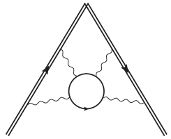
Figure 1: Diagrams contributing to the $n_{f}\mathcal{C}_{F,4}$ term in the vertex function $V(\phi)$. Double lines represent Wilson lines, wavy lines gluons and single lines the $n_{f}$ light quarks. Left-right mirror graphs and the diagrams with reversed light fermion flow are not displayed. The $n_{f}\mathcal{C}_{F,4}$ contributions of the latter equal the ones of their relatives shown here.

We are interested in color structures that generate the quartic Casimir $\mathcal{C}_{F,4}$ defined in eq. (1). It first appears in the QCD vertex correction $V$ at four loops and violates Casimir scaling. We will use the equality vanRitbergen:1998pn

$$\mathcal{C}_{F,4}=\frac{1}{N_{R}}\,\operatorname{tr}_{R}\big{[}T_{R}^{a}T_{R}^{b}T_{R}^{c}T_{R}^{d}\big{]}\;\operatorname{tr}_{F}\big{[}T_{F}^{a}T_{F}^{b}T_{F}^{c}T_{F}^{d}\big{]}+\ldots\,,$$ (6)

where the ellipsis in eq. (6) stands for terms that can be expressed only in terms of the quadratic Casimirs $C_{R}$, $C_{F}$ and $C_{A}$. Equation (6) also holds when the order of the adjoint color indices ($a,b,c,d$) in one of the traces on the right-hand side is interchanged arbitrarily.

The quartic Casimir $\mathcal{C}_{F,4}$ occurs in the four-loop contribution proportional to $n_{f}$. The latter denotes the number of light (massless) fermions in the fundamental representation $F$. From eq. (6) it is clear that the four-loop Feynman diagrams involving $\mathcal{C}_{F,4}$ must have a light fermion loop forming a box that is connected to the Wilson lines via four gluons. There are only six different diagram topologies of that type contributing to $V$. They are displayed in fig. 1. Counting also diagrams with reversed light fermion flow and left-right mirror graphs we arrive at a total of $18$ diagrams that contribute to the $\mathcal{C}_{F,4}$ term. Up to the three-loop order an analysis of all color structures and taking into account non-Abelian exponentiation Gatheral:1983cz ; Frenkel:1984pz makes it possible to rewrite all non-planar integrals in terms of planar integrals only Grozin:2015kna . This is not the case for the non-planar diagrams ($b$ -$f$).

Using the HQET building blocks ($i=1,2$)

$$S(k)=\frac{\hbox to0.0pt{/\hss}k}{k^{2}}\,,\quad H_{i}(k)=\frac{1}{k\cdot v_{i}-\frac{\delta}{2}}\,,\quad V_{i}(k)=\frac{1}{k^{2}}\bigg{[}\hbox to0.0pt{/\hss}v_{i}-\xi\frac{k\cdot v_{i}}{k^{2}}\hbox to0.0pt{/\hss}k\bigg{]},$$ (7)

associated with the fermion, heavy quark and gluon lines, respectively, we can write the diagrams of fig. 1 in generalized covariant gauge ($\xi=0$ corresponds to Feynman gauge) in compact form. The off-shellness $\delta/2$ in the heavy quark propagators serves as an infrared regulator Grozin:2015kna and can be interpreted as an external energy flowing in the opposite direction of the $v_{i}^{\mu}$ (indicated by the arrows in fig. 1). For the coefficients of the color factor $n_{f}\mathcal{C}_{F,4}$ we have

$$D_{a} =-g^{8}H_{1}(k_{2})H_{1}(k_{3})H_{2}(k_{2})H_{2}(k_{1})\,\operatorname{tr}\big{[}S(k_{4})V_{1}(k_{3})S(k_{4}-k_{3})V_{1}(k_{2}-k_{3})S(k_{4}-k_{2})$$

$$\quad\times V_{2}(k_{1}-k_{2})S(k_{4}-k_{1})V_{2}(-k_{1})\big{]}\,,$$ (8)

$$D_{b} =-g^{8}H_{1}(k_{2})H_{1}(k_{3})H_{1}(k_{1})H_{2}(k_{1})\,\operatorname{tr}\big{[}S(k_{4})V_{2}(k_{1})S(k_{4}-k_{1})V_{1}(k_{2}-k_{1})S(k_{4}-k_{2})$$

$$\quad\times V_{1}(k_{3}-k_{2})S(k_{4}-k_{3})V_{1}(-k_{3})\big{]}\,,$$ (9)

$$D_{c} =-g^{8}H_{1}(k_{2})H_{1}(k_{3})H_{2}(k_{2})H_{2}(k_{1})\,\operatorname{tr}\big{[}S(k_{4})V_{1}(k_{2}-k_{3})S(k_{4}-k_{2}+k_{3})V_{1}(k_{3})S(k_{4}-k_{2})$$

$$\quad\times V_{2}(k_{1}-k_{2})S(k_{4}-k_{1})V_{2}(-k_{1})\big{]}\,,$$ (10)

$$D_{d} =-g^{8}H_{1}(k_{2})H_{1}(k_{3})H_{1}(k_{1})H_{2}(k_{1})\,\operatorname{tr}\big{[}S(k_{2}-k_{4})V_{1}(k_{2}-k_{1})S(k_{1}-k_{4})V_{2}(k_{1})S(-k_{4})$$

$$\quad\times V_{1}(k_{3}-k_{2})S(k_{2}-k_{3}-k_{4})V_{1}(-k_{3})\big{]}\,,$$ (11)

$$D_{e} =-g^{8}H_{1}(k_{2})H_{1}(k_{3})H_{2}(k_{2})H_{2}(k_{1})\,\operatorname{tr}\big{[}S(k_{4})V_{1}(k_{3})S(k_{4}-k_{3})V_{2}(k_{1}-k_{2})S(k_{2}-k_{3}+k_{4}-k_{1})$$

$$\quad\times V_{1}(k_{2}-k_{3})S(k_{4}-k_{1})V_{2}(-k_{1})\big{]}\,,$$ (12)

$$D_{f} =-g^{8}H_{1}(k_{2})H_{1}(k_{3})H_{1}(k_{1})H_{2}(k_{1})\,\operatorname{tr}\big{[}S(k_{4})V_{2}(k_{1})S(k_{4}-k_{1})V_{1}(k_{3}-k_{2})S(k_{2}-k_{3}+k_{4}-k_{1})$$

$$\quad\times V_{1}(k_{2}-k_{1})S(k_{4}-k_{3})V_{1}(-k_{3})\big{]}\,.$$ (13)

The overall minus sign in the above expressions originates from the closed fermion loop. The sum of all 18 contributions to the $n_{f}\mathcal{C}_{F,4}$ term is gauge invariant and reads

$$V(\phi)\big{|}_{n_{f}\mathcal{C}_{F,4}} =2\,n_{f}\mathcal{C}_{F,4}\,\big{(}D_{a}+D_{b}+D_{c}+2D_{d}+2D_{e}+2D_{f}\big{)}\,.$$ (14)

The gauge invariance can be seen as follows: The $n_{f}\mathcal{C}_{F,4}$ contribution in eq. (14) is effectively QED-like, as all diagrams have the same color structure (no relative factors). Now, consider the subdiagrams consisting of the fermion loop and four off-shell gluons attached to it in all possible ways. If we pick out one of the gluon vertices and contract it with the four-momentum of the associated gluon the contributions from the 18 one-loop diagrams add up to zero owing to the Ward-Takahashi identity of QED, see e.g. ref. Peskin:1995ev . Despite being off-shell the gluons are therefore effectively transverse. Thus the (longitudinal) $\xi$ terms in their propagators vanish in the sum of all 18 diagrams. Moreover, renormalization group consistency requires eq. (14) to be at most $1/\epsilon$ divergent (for finite $\phi$), as there are no (UV) divergent subdiagrams involved. We will use these properties as strong cross-checks of our calculation.

In this paper we are interested in the expansion of the cusp anomalous dimension for small angle $\phi$. The calculation of the individual terms in this $\phi$ expansion is technically simpler than the calculation for arbitrary $\phi$, as there is only one external vector $v^{\mu}=v_{1}^{\mu}=v_{2}^{\mu}$ and the results are pure numbers. It can therefore be considered as a first step toward the calculation of the full angle-dependent cusp anomalous dimension, but also directly yields some relevant physical information as outlined in sec. 1.

Unlike e.g. the parallel lines limit ($\phi\to\pi$) or the light-like limit ($\phi\to i\infty$) the small angle limit is well-behaved Correa:2012nk ; Grozin:2015kna , i.e. we can safely expand in $\phi$ before integration over the loop momenta. By virtue of eq. (4) the leading order (LO) term ($\propto\phi^{0}$) vanishes.

In practice the Taylor expansion of the expressions in eqs. (8) – (13) can e.g. be done as follows: We write (in Euclidean spacetime) $v_{1}=v$, $v_{2}=\cos(\phi)v+\sin(\phi)e_{2}$ with $v^{2}=e_{2}^{2}=1$, $v\cdot e_{2}=0$ and differentiate the integrands w.r.t. $\phi$. The numerators of the resulting terms include a number of scalar products of the loop momenta $k_{i}^{\mu}$ with the unit vector $e_{2}^{\mu}$. The denominators are free of such scalar products. Upon integration therefore terms with odd numbers of $k_{i}\cdot e_{2}$, i.e. odd powers of $\phi$, vanish because of the antisymmetry of the integrand. For the terms with even numbers of $k_{i}\cdot e_{2}$ we perform a tensor reduction. After evaluation of the Dirac trace we end up with a scalar integrand that only involves the 14 independent scalar products $k_{i}^{2}$, $k_{i}\cdot k_{j}$ and $k_{i}\cdot v$. The result for each diagram can thus be expressed as a linear combination of integrals

$$G_{a_{1},\ldots,a_{14}}=e^{4\epsilon\gamma_{E}}\int\!\!\frac{\textrm{d}^{d}k_{1}}{i\pi^{d/2}}\int\!\!\frac{\textrm{d}^{d}k_{2}}{i\pi^{d/2}}\int\!\!\frac{\textrm{d}^{d}k_{3}}{i\pi^{d/2}}\int\!\!\frac{\textrm{d}^{d}k_{4}}{i\pi^{d/2}}\;\prod_{i=1}^{14}(Q_{i})^{-a_{i}}\,,$$ (15)

with

$$Q_{1}=-2k_{1}\cdot v+\delta\,,\;Q_{2}=-2k_{2}\cdot v+\delta\,,\;Q_{3}=-2k_{3}\cdot v+\delta\,,\;Q_{4}=-k_{1}^{2}\,,\;Q_{5}=-(k_{1}-k_{2})^{2}\,,\;$$

$$Q_{6}=-(k_{2}-k_{3})^{2}\,,\;Q_{7}=-k_{3}^{2}\,,\;Q_{8}=-k_{4}^{2}\,,\;Q_{9}=-(k_{1}-k_{4})^{2}\,,\;Q_{10}=-(k_{2}-k_{4})^{2}\,,\;$$

$$Q_{11}=-(k_{3}-k_{4})^{2}\,,\;Q_{12}=-(k_{2}-k_{3}-k_{4})^{2}\,,\;Q_{13}=-(k_{1}-k_{2}+k_{3}-k_{4})^{2}\,,\;$$

$$Q_{14}=-2k_{4}\cdot v+\delta\,,$$ (16)

at every order in $\phi$. The indices $a_{i}$ are integer numbers, which for $1\leq i\leq 13$ can be positive (propagators), zero, or negative (numerators), while $a_{14}\leq 0$, i.e. $Q_{14}$ only appears as a numerator in our problem. Note that for brevity we have suppressed the usual $-i0$ Feynman prescription in the $Q_{i}$, which is needed to ensure causality in Minkowski spacetime.

Figure 2: Independent integral topologies (1,2,3) for the small angle expansion of $V(\phi)$. The number $i$ for each (double) line refers to the corresponding propagator with power $a_{i}$ in $G_{a_{1},\ldots,a_{14}}$ according to eq. (15). Propagators 1,2,3 are (linear) Wilson line (heavy quark) propagators.

The integrals $G$ contributing to the vertex function $V$ have at most 11 propagators. According to its propagator configuration each of them can be assigned to one of the integral topologies displayed in fig. 2. The natural way to do this is to map the small angle expanded diagrams $D_{a,d}$ onto topology 1, $D_{b,e}$ onto topology 2, and $D_{c,f}$ onto topology 3. We can now perform an integration-by-parts (IBP) reduction Chetyrkin:1981qh for the integrals of each topology separately. We do this reduction to master integrals (MI) for all relevant integrals up to $\mathcal{O}\!\left(\phi^{4}\right)$. To this end, we use the public computer program FIRE5 Smirnov:2014hma in combination with LiteRed Lee:2012cn ; Lee:2013mka . In this way, we find 32 MI for topology 1, 32 MI for topology 2 and 30 MI for topology 3. Taking into account relations among the MI of different topologies (with less than 11 propagators), the total number of independent MI across the three topologies is 43. Expressing the $\phi$-expanded vertex function $V$ as a linear combination of these 43 MI, we explicitly verify that the $\xi$-dependence in the coefficients of the MI drops out at $\mathcal{O}\!\left(\phi^{0}\right)$ and $\mathcal{O}\!\left(\phi^{2}\right)$ as required by gauge invariance. At order $\mathcal{O}\!\left(\phi^{4}\right)$, we restrict ourselves to the Feynman gauge for performance reasons. We note that the extension to higher powers of $\phi$ is conceptionally straightforward, and is only limited by computing resources.

As the final step of our calculation we have to solve the MI to sufficiently high order in $\epsilon$ in order to determine the overall $1/\epsilon$ divergence of $V$ related to the cusp anomalous dimension via eq. (5). For the computation of the MI we use the HyperInt package Panzer:2014caa . This code allows to automatically evaluate linearly reducible convergent Feynman integrals in terms of multiple polylogarithms. In our case the latter reduces to transcendental numbers.

In order to provide finite Feynman parameter integrals as an input to HyperInt we first switch to a MI basis without divergent subintegrals (except for trivial bubble insertions that can be integrated out.) In practice this is done by inserting a sufficient number of dots on the (off-shell) heavy quark lines of the MI, i.e. by increasing the power of the linear propagators by an integer amount. The resulting new basis of MI is then related to the old one by IBP reduction. Next, we Fourier transform to position space and directly integrate out the simple bubble and HQET self-energy subintegrals by hand. This effectively produces integrals with non-integer $\epsilon$-dependent propagator powers, but less than four loops. In order to avoid generating new divergent subintegrals in this process, it may be necessary to increase the powers also of some of the involved bubble propagators beforehand. The resulting integrals all have at most one overall UV divergence ($\propto 1/\epsilon$).

Without loss of generality we can fix the position of the left-most vertex on the Wilson line to the coordinate origin ($x_{1}=0$) and parametrize the following vertices from left to right along the Wilson line by $\rho\,x_{2}$, $\rho(x_{2}+x_{3})$, etc., where $0\leq x_{i}\leq 1$, $\sum_{i}x_{i}=1$. The parameter $\rho$ has the dimension of a length and $0\leq\rho\leq\infty$. We can now write down a Feynman parameter representation for the integral over the positions of the non-Wilson-line vertices as a function of the $x_{i}$ and $\rho$. In particular its dependence on the only dimensionful parameter, $\rho$, can be easily deduced from dimensional power counting. The position space representation of a HQET Wilson line propagator between the vertices $l$ and $m$ of arbitrary power $a$ reads

$$\int\frac{\textrm{d}q}{2\pi}\;\frac{e^{-iq\rho\,x_{m}}}{(-2q+\delta)^{a}}=\left(\frac{i}{2}\right)^{\!\!a}\frac{1}{\Gamma(a)}\,\rho^{a-1}\,x_{m}^{a-1}\,e^{-ix_{m}\rho\,\delta/2}\,.$$ (17)

Note that because of the causal $-i0$ prescription $\delta$ can be considered to have an infinitesimally small negative imaginary part. The remaining overall UV divergence, if present, originates from the integration region, where all vertices on the Wilson line are contracted to one point, i.e. where $\rho\to 0$, cf. ref. Grozin:2015kna . In our parametrization, the product of all heavy quark propagators in a diagram together with the $\rho$-dependence from the Feynman parameter integral thus yields $\rho^{z}\exp(-i\rho\,\delta/2)$. The power $z$ only depends on $\epsilon$ and is fixed by the dimensionality of the MI. The possibly divergent $\rho$ integral can therefore be carried out easily. We have thus factored out the UV divergences completely and are left with a convergent integral over Feynman parameters and the $x_{i}$. Its integrand can now safely be expanded in $\epsilon$. The individual terms in this expansion are then computed with HyperInt.

Let us illustrate this procedure for the following non-planar nine-propagator MI (number 38 in our list):

$$\text{MI}_{38}=\!\raisebox{-11.38109pt}{\includegraphics[width=113.81102pt]{diagpics/MI37.pdf}}\!=G_{1,2,1,1,0,1,1,0,1,1,0,1,0,0}=(4\pi)^{2d}e^{2\gamma_{E}(4-d)}\!\int_{0}^{\infty}\!\!\textrm{d}\rho\rho^{2}\int_{0}^{1}\!\textrm{d}x_{1}$$

$$\times\int_{0}^{1-x_{1}}\!\!\textrm{d}x_{2}\,\bigg{[}\frac{1}{16}\,\rho\,x_{2}\,e^{-i\delta\rho/2}\bigg{]}\int\prod_{i=1}^{6}\textrm{d}\alpha_{i}\bigg{[}\frac{\pi^{-2d}\Gamma(2d-6)}{4096}(\alpha_{1}\alpha_{2}\alpha_{3}\alpha_{4}\alpha_{5}\alpha_{6})^{\frac{d-4}{2}}F^{6-2d}U^{\frac{3}{2}d-6}\bigg{]},$$ (18)

where

$$F =(-\rho^{2})\bigg{\{}\alpha_{1}\alpha_{2}(\alpha_{3}+\alpha_{4}+\alpha_{5}+\alpha_{6})(1-x_{1})^{2}+\alpha_{6}\Big{(}\alpha_{1}\alpha_{3}x_{1}^{2}+\alpha_{4}\big{[}\alpha_{2}(1-x_{1})^{2}+\alpha_{3}x_{1}^{2}\big{]}$$

$$\quad+\alpha_{5}\big{[}\alpha_{1}x_{2}^{2}+\alpha_{4}x_{2}^{2}+\alpha_{2}(1-x_{1}-x_{2})^{2}+\alpha_{3}(x_{1}+x_{2})^{2}\big{]}+\alpha_{2}\alpha_{3}\Big{)}$$

$$\quad+(\alpha_{1}+\alpha_{2})\Big{(}\alpha_{4}\alpha_{5}x_{2}^{2}+\alpha_{3}\big{[}\alpha_{4}x_{1}^{2}+\alpha_{5}(x_{1}+x_{2})^{2}\big{]}\Big{)}\bigg{\}}\,,$$ (19)

$$U =(\alpha_{1}+\alpha_{2})(\alpha_{3}+\alpha_{4}+\alpha_{5})+(\alpha_{1}+\alpha_{2}+\alpha_{3}+\alpha_{4}+\alpha_{5})\alpha_{6}\,.$$ (20)

We have inserted a dot on the middle heavy quark line in order to render the two- and three-loop subintegrals finite. The first expression in squared brackets in eq. (18) arises from the product of the three Wilson line propagators according to eq. (17) (for the middle one $a=2$). The second term in squared brackets corresponds to the Feynman parameter ($\alpha_{i}$) representation of the integration over the two internal space-time vertices (the ones not lying on the Wilson line). Doing the $\rho$ integral yields a factor ($\delta\to\delta-i0$)

$$\int_{0}^{\infty}\!\textrm{d}\rho\,\rho^{3}\,\big{(}\!-\!\rho^{2}\big{)}^{6-2d}\,e^{-i\delta\rho/2}=\Gamma(16-4d)\,\bigg{(}\frac{\delta}{2}\bigg{)}^{\!\!4(d-4)},$$ (21)

which is $1/\epsilon$ (UV) divergent. The $\alpha$-integrations in eq. (18) are projective, see e.g. Smirnov:2006ry , and we use this freedom to choose $\alpha_{1}\equiv 1$. With this choice the other Feynman parameters are integrated from zero to infinity. After expansion in $\epsilon$ we evaluate these convergent integrals together with the ones over $x_{1}$ and $x_{2}$ using HyperInt. The result is

$$\text{MI}_{38} =\frac{1}{\epsilon}\bigg{(}\frac{\pi^{2}\zeta_{3}}{12}+\frac{5\zeta_{5}}{2}\bigg{)}+5\zeta_{5}-\frac{17\zeta_{3}^{2}}{2}+\frac{\pi^{2}\zeta_{3}}{6}-\frac{169\pi^{6}}{6480}+\mathcal{O}\!\left(\epsilon\right)\,.$$ (22)

Here we have set the IR regulator $\delta=1$ for convenience. This will not affect the final result for the cusp anomalous dimension. Also the $\mathcal{O}\!\left(\epsilon\right)$ term in eq. (22) will not contribute to $\Gamma_{\rm cusp}(\phi)$ through $\mathcal{O}\!\left(\phi^{4}\right)$, as can be verified by inspection of the overall $\epsilon$-dependent coefficient of MI₃₈ in the IBP reduced expressions for the vertex function.

With the methods described above we have computed all MI to the relevant order in $\epsilon$. This, in particular, includes the three eleven-propagator MI corresponding to the maximal graphs (with single propagator powers) of the three integral topologies in fig. 2. For the latter already the leading term in the $\epsilon$ expansion turns out to be sufficient. We have checked our analytic results numerically with FIESTA Smirnov:2015mct . A list of the results for the MI in electronic form can be found in the ancillary file of the present paper.

For a number of MI it is straightforward to derive four-fold Mellin–Barnes representations by applying the two-fold representation for the heavy–light vertex Davydychev:2001ui twice. They can be transformed to a four-fold series, which can be used to obtain the expansions in $\epsilon$. We however find this method less convenient than the procedure described above.

3 The HQET heavy-quark field anomalous dimension

Let us denote the heavy quark self energy ($i$ times the sum of all 1PI heavy quark self-energy diagrams) by $\Sigma_{h}$, and the external heavy quark energy by $\omega$. In our configuration $\omega=-\delta/2$. The HQET (off-shell) Ward identity then relates $\Sigma_{h}$ to the vertex function at zero angle via

$$V(0) =1-\frac{\partial\Sigma_{h}(\omega)}{\partial\omega}\,.$$ (23)

In fact, we have employed this identity already in eq. (4). Hence, we can write

$$\log V(0)=-\log Z_{h}+\mathcal{O}\!\left(\epsilon^{0}\right)\,,$$ (24)

where $Z_{h}$ is the ($\overline{\rm MS}$) heavy quark wave function renormalization factor and $V(0)$ is expressed in terms of the renormalized coupling $\alpha_{s}(\mu)$ and gauge parameter $\xi(\mu)$. We thus have

$$\gamma_{h}\big{|}_{n_{f}\mathcal{C}_{F,4}}\equiv\frac{\textrm{d}\log Z_{h}}{\textrm{d}\log\mu}\Big{|}_{n_{f}\mathcal{C}_{F,4}}=8\epsilon V(0)\big{|}_{n_{f}\mathcal{C}_{F,4}}+\mathcal{O}\!\left(\epsilon\right)$$ (25)

for the $n_{f}\mathcal{C}_{F,4}$ term of the associated anomalous dimension $\gamma_{h}$, which determines the running of the renormalized HQET heavy quark field $h$ through the renormalization group equation

$$\frac{\textrm{d}}{\textrm{d}\log\mu}\,h(\mu)=-\frac{\gamma_{h}}{2}\,h(\mu)\,.$$ (26)

As field renormalization is irrelevant to physical observables $\gamma_{h}$ can depend on the gauge. The gauge dependence has been explicitly shown at three loops, where the complete result is known Melnikov:2000zc ; Chetyrkin:2003vi . Unlike other parts, the four-loop $n_{f}\mathcal{C}_{F,4}$ term, however, is gauge invariant for the reason discussed above. For $\phi=0$ our calculation of the vertex function yields

$$\gamma_{h}\big{|}_{n_{f}\mathcal{C}_{F,4}}=n_{f}\mathcal{C}_{F,4}\bigg{(}\frac{\alpha_{s}}{\pi}\bigg{)}^{\!\!4}\biggl{(}\!\!-\frac{5}{4}\zeta_{5}+\frac{2}{3}\pi^{2}\zeta_{3}+\zeta_{3}-\frac{2}{3}\pi^{2}\biggr{)}\,.$$ (27)

We have also calculated the $n_{f}\mathcal{C}_{F,4}$ term of $\Sigma_{h}$ from HQET heavy quark self energy diagrams (without cusp) and checked explicitly that eq. (23) is fulfilled.

The $\overline{\rm MS}$ renormalized QCD heavy-quark field $Q$ is related to the $\overline{\rm MS}$ renormalized HQET field $h$ by the matching relation Grozin:2010wa

$$Q(\mu) =z(\mu)^{1/2}h(\mu)+\mathcal{O}\!\left(\frac{1}{m}\right),$$ (28)

$$z(\mu) =\frac{Z_{h}\Big{(}\alpha_{s}^{(n_{f})}(\mu),\xi^{(n_{f})}(\mu)\Big{)}Z_{Q}^{\text{os}}\Big{(}g_{0}^{(n_{f}+1)},\xi_{0}^{(n_{f}+1)}\Big{)}}{Z_{Q}\Big{(}\alpha_{s}^{(n_{f}+1)}(\mu),\xi^{(n_{f}+1)}(\mu)\Big{)}Z_{h}^{\text{os}}\Big{(}g_{0}^{(n_{f})},\xi_{0}^{(n_{f})}\Big{)}}\,.$$ (29)

The $Z_{i}$ and $Z_{i}^{\rm os}$ denote the renormalization factors for the field $i=Q,h$ in the $\overline{\rm MS}$ and on-shell scheme, respectively. Bare quantities are labeled by a subscript 0 and $\xi(\mu)$ is the $\overline{\rm MS}$ renormalized gauge parameter: $1-\xi_{0}=Z_{A}\big{(}\alpha_{s}(\mu),\xi(\mu)\big{)}\big{(}1-\xi(\mu)\big{)}$ with $Z_{A}$ being the $\overline{\rm MS}$ renormalization factor of the gluon field. The superscripts on the couplings and $\xi$ indicate the number of active flavors in the theory.

If we take all $n_{f}$ light flavors to be massless, we have $Z_{h}^{\text{os}}=1$, because the HQET self-energy diagrams are scaleless in the on-shell limit, i.e. for $\omega\to 0$. The four-loop $n_{f}\mathcal{C}_{F,4}$ term in the anomalous dimension $\gamma_{Q}$ is known Czakon:2004bu :

$$\gamma_{Q}\big{|}_{n_{f}\mathcal{C}_{F,4}} \equiv\frac{\textrm{d}\log Z_{Q}}{\textrm{d}\log\mu}\Big{|}_{n_{f}\mathcal{C}_{F,4}}=n_{f}\mathcal{C}_{F,4}\bigg{(}\frac{\alpha_{s}}{\pi}\bigg{)}^{\!\!4}\,,$$ (30)

and we can thus determine $Z_{Q}$. The on-shell heavy-quark field renormalization constant $Z_{Q}^{\text{os}}$ is known up to three loops Melnikov:2000zc . As $z(\mu)$ must be finite in the limit $\epsilon\to 0$ we then find

$$Z_{Q}^{\text{os}}\big{|}_{n_{f}\mathcal{C}_{F,4}}=n_{f}\mathcal{C}_{F,4}\frac{g_{0}^{8}m_{\text{os}}^{-8\epsilon}}{(4\pi)^{2d}}\left[-\frac{8}{\epsilon}\left(5\zeta_{5}-\frac{8}{3}\pi^{2}\zeta_{3}-4\zeta_{3}+\frac{8}{3}\pi^{2}+4\right)+\mathcal{O}(\epsilon^{0})\right]\,.$$ (31)

This result can be used as a check of a future four-loop calculation of $Z_{Q}^{\rm os}$.

4 Result for the cusp anomalous dimension

Putting all pieces together we obtain

$$\Gamma_{\rm cusp}\big{|}_{n_{f}\mathcal{C}_{F,4}}={} n_{f}\mathcal{C}_{F,4}\bigg{(}\frac{\alpha_{s}}{\pi}\bigg{)}^{\!\!4}\frac{1}{9}\Bigg{[}\phi^{2}\bigg{(}\!\!-4\pi^{2}\zeta_{3}+\frac{5}{12}\pi^{4}+\frac{5}{6}\pi^{2}\bigg{)}$$

$${}+\phi^{4}\bigg{(}\!\!-4\zeta_{5}-\frac{16}{75}\pi^{2}\zeta_{3}+\frac{71}{25}\zeta_{3}+\frac{49}{900}\pi^{4}-\frac{157}{900}\pi^{2}-\frac{23}{100}\bigg{)}+\mathcal{O}\!\left(\phi^{6}\right)\Bigg{]}\,$$ (32)

$$={} n_{f}\mathcal{C}_{F,4}\bigg{(}\frac{\alpha_{s}}{\pi}\bigg{)}^{\!\!4}\Big{[}0.150721\,\phi^{2}+0.00965191\,\phi^{4}+\mathcal{O}\!\left(\phi^{6}\right)\Big{]}\,,$$ (33)

while the conjecture from refs. Grozin:2014hna ; Grozin:2015kna predicts

$$\Gamma_{\rm cusp}\big{|}_{n_{f}\mathcal{C}_{F,4}}^{\text{conjecture}}={} n_{f}\mathcal{C}_{F,4}\bigg{(}\frac{\alpha_{s}}{\pi}\bigg{)}^{\!\!4}\frac{1}{192}\biggl{(}\phi^{2}+\frac{\phi^{4}}{15}+\mathcal{O}\!\left(\phi^{6}\right)\biggr{)}\bigg{(}16\pi^{4}\log^{2}2-336\pi^{2}\zeta_{3}\log 2$$

$${}-\frac{16}{3}\pi^{4}\log 2-32\pi^{2}\log 2+\frac{488}{3}\pi^{2}\zeta_{3}-\frac{5}{3}\pi^{6}+\frac{92}{3}\pi^{4}-\frac{632}{9}\pi^{2}\bigg{)}$$ (34)

$$={} n_{f}\mathcal{C}_{F,4}\bigg{(}\frac{\alpha_{s}}{\pi}\bigg{)}^{\!\!4}\Big{[}0.14801\,\phi^{2}+0.00986736\,\phi^{4}+\mathcal{O}\!\left(\phi^{6}\right)\Big{]}$$ (35)

with input from the analytic three-loop static potential Lee:2016cgz .

We see from our result, eq. (32), that the relative coefficients of the $\phi^{2}$ and $\phi^{4}$ terms differ from the conjectured form, eq. (34). Moreover, taking into account the analytic form of the static quark anti-quark potential, we see that the latter involves transcendental constants such as $\log 2$ that do not appear in our four-loop MI. All of this suggests that the full function $\Gamma_{\rm cusp}(\phi)$ takes a more complicated form, so that it can reproduce these features.

Nevertheless, it is interesting to compare the numerical size of the contributions. The exact expression in eq. (33) and the (wrong) conjecture in eq. (35) are numerically remarkably close.

- (1) A. M. Polyakov, Gauge Fields as Rings of Glue, Nucl. Phys. B164 (1980) 171–188.
- (2) A. F. Falk, H. Georgi, B. Grinstein, and M. B. Wise, Heavy meson form-factors from QCD, Nucl. Phys. B343 (1990) 1–13.
- (3) Y. Amhis et al., Averages of -hadron, -hadron, and -lepton properties as of summer 2016, arXiv:1612.07233.
- (4) A. Czarnecki, K. Melnikov, and N. Uraltsev, Nonabelian dipole radiation and the heavy quark expansion, Phys. Rev. Lett. 80 (1998) 3189–3192, [hep-ph/9708372].
- (5) D. Correa, J. Henn, J. Maldacena, and A. Sever, An exact formula for the radiation of a moving quark in N=4 super Yang Mills, JHEP 06 (2012) 048, [arXiv:1202.4455].
- (6) G. P. Korchemsky and A. V. Radyushkin, Renormalization of the Wilson loops beyond the leading order, Nucl. Phys. B283 (1987) 342–364.
- (7) D. Correa, J. Henn, J. Maldacena, and A. Sever, The cusp anomalous dimension at three loops and beyond, JHEP 05 (2012) 098, [arXiv:1203.1019].
- (8) A. Grozin, J. M. Henn, G. P. Korchemsky, and P. Marquard, Three loop cusp anomalous dimension in QCD, Phys. Rev. Lett. 114 (2015), no. 6 062006, [arXiv:1409.0023].
- (9) A. Grozin, J. M. Henn, G. P. Korchemsky, and P. Marquard, The three-loop cusp anomalous dimension in QCD and its supersymmetric extensions, JHEP 01 (2016) 140, [arXiv:1510.07803].
- (10) T. van Ritbergen, A. N. Schellekens, and J. A. M. Vermaseren, Group theory factors for Feynman diagrams, Int. J. Mod. Phys. A14 (1999) 41–96, [hep-ph/9802376].
- (11) C. Anzai, Y. Kiyo, and Y. Sumino, Violation of Casimir scaling for static QCD potential at three-loop order, Nucl. Phys. B838 (2010) 28–46, [arXiv:1004.1562]. [Erratum: Nucl. Phys.B890,569(2015)].
- (12) R. N. Lee, A. V. Smirnov, V. A. Smirnov, and M. Steinhauser, Analytic three-loop static potential, Phys. Rev. D94 (2016), no. 5 054029, [arXiv:1608.02603].
- (13) R. H. Boels, T. Huber, and G. Yang, The four-loop non-planar cusp anomalous dimension in SYM, arXiv:1705.03444.
- (14) C. Anzai, Y. Kiyo, and Y. Sumino, Static QCD potential at three-loop order, Phys. Rev. Lett. 104 (2010) 112003, [arXiv:0911.4335].
- (15) A. V. Smirnov, V. A. Smirnov, and M. Steinhauser, Three-loop static potential, Phys. Rev. Lett. 104 (2010) 112002, [arXiv:0911.4742].
- (16) S. Moch, B. Ruijl, T. Ueda, J. A. M. Vermaseren, and A. Vogt, Four-Loop Non-Singlet Splitting Functions in the Planar Limit and Beyond, arXiv:1707.08315.
- (17) K. Melnikov and T. van Ritbergen, The three loop on-shell renormalization of QCD and QED, Nucl. Phys. B591 (2000) 515–546, [hep-ph/0005131].
- (18) K. G. Chetyrkin and A. G. Grozin, Three loop anomalous dimension of the heavy–light quark current in HQET, Nucl. Phys. B666 (2003) 289–302, [hep-ph/0303113].
- (19) J. M. Henn and T. Huber, The four-loop cusp anomalous dimension in 4 super Yang-Mills and analytic integration techniques for Wilson line integrals, JHEP 09 (2013) 147, [arXiv:1304.6418].
- (20) J. G. M. Gatheral, Exponentiation of eikonal cross-sections in nonabelian gauge theories, Phys. Lett. 133B (1983) 90–94.
- (21) J. Frenkel and J. C. Taylor, Nonabelian eikonal exponentiation, Nucl. Phys. B246 (1984) 231–245.
- (22) M. E. Peskin and D. V. Schroeder, An introduction to quantum field theory. 1995.
- (23) K. G. Chetyrkin and F. V. Tkachov, Integration by parts: The algorithm to calculate functions in 4 loops, Nucl. Phys. B192 (1981) 159–204.
- (24) A. V. Smirnov, FIRE5: a C++ implementation of Feynman Integral REduction, Comput. Phys. Commun. 189 (2015) 182–191, [arXiv:1408.2372].
- (25) R. N. Lee, Presenting LiteRed: a tool for the Loop InTEgrals REDuction, arXiv:1212.2685.
- (26) R. N. Lee, LiteRed 1.4: a powerful tool for reduction of multiloop integrals, J. Phys. Conf. Ser. 523 (2014) 012059, [arXiv:1310.1145].
- (27) E. Panzer, Algorithms for the symbolic integration of hyperlogarithms with applications to Feynman integrals, Comput. Phys. Commun. 188 (2015) 148–166, [arXiv:1403.3385].
- (28) V. A. Smirnov, Feynman integral calculus. 2006.
- (29) A. V. Smirnov, FIESTA4: Optimized Feynman integral calculations with GPU support, Comput. Phys. Commun. 204 (2016) 189–199, [arXiv:1511.03614].
- (30) A. I. Davydychev and A. G. Grozin, HQET quark - gluon vertex at one loop, Eur. Phys. J. C20 (2001) 333–342, [hep-ph/0103078].
- (31) A. G. Grozin, Matching heavy-quark fields in QCD and HQET at three loops, Phys. Lett. B692 (2010) 161–165, [arXiv:1004.2662].
- (32) M. Czakon, The four-loop QCD -function and anomalous dimensions, Nucl. Phys. B710 (2005) 485–498, [hep-ph/0411261].