APFEL++: A new PDF evolution library in C++

Abstract:

I present a preliminary version of APFEL++, a C++ rewriting of the Fortran 77 evolution code APFEL. In this contribution I discuss the new philosophy adopted for the numerical computation of the convolutions, demonstrate the ability to reproduce old results in an accurate and fast way, and present an original application to the computation of the semi-inclusive deep-inelastic-scattering cross section to next-to-leading order in QCD.

Introduction.

In the LHC era the need for modern and fast tools for the analysis of the experimental data is constantly rising. Indeed, meeting the increasingly high precision of the data entails the growth of the complexity of the tasks to be carried out to produce accurate predictions. This often leads existing codes to be continuously updated with the implementation of new features. This causes an inevitable stratification that makes the maintenance and the development of such codes increasingly cumbersome.

Since its born, the APFEL code [1] has undergone a large number of developments used in many studies (see e.g. Refs. [18, 17, 16, 15, 14, 13, 12]) and that have led it way beyond the purposes for which it was originally conceived. In addition, APFEL is coded in Fortran 77. This is a perfectly appropriate language for relatively small programs but lacks of modularity and of tools for an optimal management of memory and thus it is not suitable for larger projects. These limitations were compelling reasons to re-think and re-implement APFEL from scratch having in mind the wider range of applications of the new code.

Basic design of the code.

The coding language used to write APFEL++ is C++ as it ensures modularity, through the definition of objects, and allows for a dynamic management of memory. We have chosen to use the C++11 official standard that, as compared to the older major standards, offers a number of very useful tools and is currently well supported by modern compilers.

The basic idea behind the structure of the new code is that of defining a limited number of building blocks that can be used to construct more complex quantities. The central observation is that, in the context of collinear factorisation, a relevant quantity $M$ is typically computed as a Mellin convolution between an operator $O$ and a distribution $d$:

$$\small M(x)=\int_{0}^{1}dy\int_{0}^{1}dz\,O(y)d(z)\delta(x-yz)=\int_{x}^{1}\frac{dy}{y}\,O(y)d\left(\frac{x}{y}\right)=\int_{x}^{1}\frac{dz}{z}\,O\left(\frac{x}{z}\right)d(z)\equiv O(x)\otimes d(x)\,.$$ (1)

The operator $O$ is typically a process-dependent perturbative expression that usually contains: “regular” terms whose integration in Eq. (1) does not present any complication, “local” terms proportional to $\delta(1-x)$, and “singular” terms whose singularity in $x=1$ is subtracted by means of the so-called plus-prescription. When going to higher perturbative orders, this kind of expressions may become rather convoluted and make the numerical integration expensive. The distribution $d$, instead, is usually a simple function, $e.g.$ a parton distribution or a fragmentation function, that contains information on the universal non-perturbative dynamics of some hadron. The function $d$ is typically fast to access, $e.g.$ through the LHAPDF interface [2], and thus is much less expensive than the operator $O$ in the integral in Eq. (1).

The common strategy to make the computation of integrals such as that in Eq. (1) fast is that of using interpolation techniques to precompute the expensive part. More specifically, the integration variable $z$ is discretised by means of a grid $g\equiv\{z_{0},\dots,z_{N_{z}}\}$ and the distribution $d$ is interpolated using a moving set of interpolating functions:

$$d(z)=\sum_{\beta\in g}w_{\beta}(z)d_{\beta}\,,$$ (2)

where $d_{\beta}\equiv d(z_{\beta})$ is the value of the distribution $d$ on the $\beta$-th node of the grid and $w_{\beta}$ is the interpolating function associated to that node, $e.g.$ a Lagrange polynomial. Plugging Eq. (2) into Eq. (1) and assuming the value of $x$ to be equal to the $\alpha$-th grid node, we find:

$$M_{\alpha}\equiv M(x_{\alpha})=O_{\alpha\beta}d_{\beta}\quad\mbox{with}\quad O_{\alpha\beta}\equiv\int_{x_{\alpha}}^{1}\frac{dy}{y}O(y)w_{\beta}\left(\frac{x_{\alpha}}{y}\right)\,,$$ (3)

where a sum over repeated greek indices is now understood. The value of $M$ for an arbitrary value of $x$ can then be obtained through interpolation using Eq. (2). Once the integral in the r.h.s. of Eq. (3) has been computed, the convolution just amounts of a multiplication between a matrix and a vector. This operation is very fast and allows one to recompute the function $M$ with different distributions $d$ very quickly.

We are now able to identify the building blocks we were looking for:

• the grid $g$, that is the set of nodes over a relevant range in the integration variable and of the interpolating functions associated to each node,

• the distribution $\{d_{\beta}\}$, $i.e.$ the set of the values of the function $d(x)$ on the nodes of $g$,

• the operator $\{O_{\alpha\beta}\}$, that is the set of values of the integral in the r.h.s. of Eq. (3) for all indices $\alpha$ and $\beta$, both running on the nodes of $g$.

Therefore, the primary functionality of the code is the construction of these three objects. It is interesting to notice that Eq. (3) reduces the Mellin convolution in Eq. (1) to a simple problem of linear algebra and as such all the properties of linear transformations hold. More in particular, Eq. (3) shows that $M_{\alpha}$ belongs to the category of distributions like $d_{\beta}$. In other words, in this context a physical observable is also identified with a distribution. In the next section I will show how the ingredients listed above are sufficient for a number of interesting applications.

Applications.

The original purpose of APFEL was the solution of the DGLAP evolution equations in the factorisation scale $\mu$ that, in the framework discussed above, reduce to:

$$\frac{{\rm d}{\bf f}_{\alpha}}{{\rm d}t}={\bf\overline{P}}_{\alpha\beta}\cdot{\bf f}_{\beta}\,.$$ (4)

with $t=\ln\mu^{2}$ and where ${\bf f}_{\alpha}$ is a vector of distributions in the quark-flavour space, corresponding to the parton distribution functions (PDFs) or to the fragmentation functions (FFs) of the different partonic species, and ${\bf\overline{P}}_{\alpha\beta}$ is instead a matrix of operators in the quark-flavour space, corresponding to the splitting functions. The dot in the r.h.s. of Eq. (4) represents the product in flavour space between the matrix ${\bf\overline{P}}$ and the vector f that gives rise to another vector. Eq. (4) is a linear ordinary differential equation in ${\bf f}_{\alpha}$ that can be solved using, for example, the Runge-Kutta method.

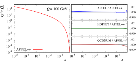
Figure 1: The gluon PDF at 100 GeV. Left panel: distribution evolved in NNLO QCD with APFEL++. Right panels: ratios to APFEL++ of the same distribution evolved with: APFEL (upper plot), HOPPET [6] (central plot), and QCDNUM [7] (lower plot). The initial conditions for are those of Ref. [8].

As a practical application, Fig. 1 displays the gluon PDF evolved to $Q=100$ GeV at NNLO in QCD starting from the initial conditions given in Ref. [8]. The result obtained with APFEL++ and shown in the left panel, is compared to the three public codes: APFEL, HOPPET [6], and QCDNUM [7]. The agreement between all these codes is excellent with very small deviations mostly arising from the different interpolation strategies.

The computation of the deep-inelastic-scattering (DIS) structure functions in $ep$ collisions can also be addressed using the same technology. In this case, the observable $F$ can be computes as:

$$F_{\alpha}={\bf C}_{\alpha\beta}\cdot{\bf f}_{\beta}\,,$$ (5)

where ${\bf f}_{\alpha}$ is a vector of distributions in flavour space, corresponding to the relevant combinations of PDFs, and ${\bf C}_{\alpha\beta}$ is also a vector in flavour space but of operators, corresponding to the coefficient functions. The dot in the r.h.s now indicates the inner product in flavour space between ${\bf C}$ and ${\bf f}$ that gives rise to the scalar $F$.

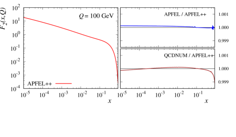
Figure 2: The structure function $F_{2}$ at 100 GeV. Left panel: $F_{2}$ in NNLO QCD with APFEL++. Right panels: ratios to APFEL++ of the same observable computed with: APFEL (upper plot), and QCDNUM [7] (lower plot).

Fig. 2 displays the prediction for the DIS structure function $F_{2}$ at NNLO in QCD computed at $Q=100$ GeV. The result obtained with APFEL++ is shown in the left panel and compared to APFEL and QCDNUM in the right panels. The agreement between these codes is again extremely good.

The method described above applies also to the convolution of two operators, $O^{(1)}$ and $O^{(2)}$, that gives as a result to a third operator $O^{(3)}$, as follows:

$$O^{(3)}_{\alpha\beta}=O^{(1)}_{\alpha\gamma}O^{(2)}_{\gamma\beta}=O^{(2)}_{\alpha\gamma}O^{(1)}_{\gamma\beta}\,,$$ (6)

where the last equality follows from the definition of operator in Eq. (3). This kind of products is relevant when considering factorisation scale variations that typically generate terms involving convolutions between hard cross sections and splitting functions.

As an example, I have computed the convolution:

$$\left[P_{qq}^{(0)}(x)\otimes P_{qq}^{(0)}(x)\right]\otimes f(x)\,,\quad\mbox{with}\quad P_{qq}^{(0)}(x)=\left(\frac{1+x^{2}}{1-x}\right)_{+}\quad\mbox{and}\quad\underbrace{f(x)=1-x}_{\mbox{\small test function}}\,,$$ (7)

both numerically, using the method discussed above, and analytically, knowing that:

$$\small P_{qq}^{(0)}(x)\otimes P_{qq}^{(0)}(x)=\left(\frac{4(x^{2}+1)\ln(1-x)+x^{2}+5}{1-x}\right)_{+}-\frac{(3x^{2}+1)\ln x}{1-x}-4+\left(\frac{9}{4}-\frac{2\pi^{2}}{3}\right)\delta(1-x)\,.$$ (8)

Fig. 3 shows an excellent agreement between the numerical and the analytical computations, demonstrating that the numerical convolution is very accurate over all the considered range.

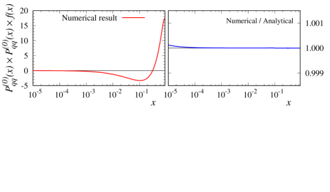
Figure 3: Representation of Eq. (7). The left panel displays the result obtained computing the convolution $P_{qq}^{(0)}(x)\otimes P_{qq}^{(0)}(x)$ numerically while the right panel shows the ratio to the result obtained using the analytical expression in Eq. (8).

Finally, this technology turns out to be useful also in the presence of convolutions over more than one variable. Two interesting examples are the computation of the Drell-Yan and of the semi-inclusive DIS (SIDIS) cross sections. In this case, the typical integrals to compute have the form:

$$D(x,z)=\int_{x}^{1}\frac{d\xi}{\xi}\int_{z}^{1}\frac{d\zeta}{\zeta}\,O\left(\frac{x}{\xi},\frac{z}{\zeta}\right)\,d^{(1)}(\xi)\,d^{(2)}(\zeta)\,.$$ (9)

Restricting ourselves to the computation of these cross sections to $\mathcal{O}(\alpha_{s})$, $i.e.$ next-to-leading order in QCD, a simple inspection reveals that the expressions of the hard cross sections [3, 4], represented by the “double” function $O$ in Eq. (9), can be decomposed as follows:

$$O(x,z)=\sum_{i}K_{i}C_{i}^{(1)}(x)C_{i}^{(2)}(z)\,,$$ (10)

where $K_{i}$ are numerical factors, while $C_{i}^{(1)}$ and $C_{i}^{(2)}$ are “single” functions of the variables $x$ and $z$. This allows for a simple extension of the procedure discussed above so that:

$$D_{\alpha\beta}\equiv D(x_{\alpha},z_{\delta})=\sum_{i}K_{i}\left[O_{i,\alpha\gamma}^{(1)}d_{\gamma}^{(1)}\right]\left[O_{i,\beta\delta}^{(2)}d_{\delta}^{(2)}\right]\,,$$ (11)

that is a bilinear combination of single operators. This combination greatly reduces the complexity of the computation of the double integral in Eq. (9) and thus makes it much faster.

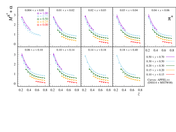
Figure 4: Comparison between the SIDIS multiplicities for $\pi^{+}$ measured by COMPASS and the [9] and the NLO predictions computed with APFEL++ using the MSTW2008 PDF set [10] and the DSS14 FF set [11].

I have applied this strategy to the computation of the SIDIS multiplicities. In Fig. 4 the NLO predictions for $\pi^{+}$ production obtained with APFEL++ using the MSTW2008 PDF set [10] and the DSS14 FF set [11] are compared to the COMPASS data [9]. Since these measurements have been made public very recently, they have not been included in any FF analysis yet. However, the predictions obtained with APFEL++ are in fair agreement with the data.

Performance.

The main foreseeable application of APFEL++ is in fits of PDFs and/or FFs, where a large number of predictions have to be produced very quickly in order to ensure that the fits converge in a reasonable amount of time. Therefore, a lot of effort has been put to make the computation of the evolution and of the observables as fast as possible. To this purpose, APFEL++ implements a method to tabulate operators and distributions over a grid in the scale $Q$ in such a way that quantities that depend on both $x$ and $Q$, like PDFs/FFs and structure functions, are obtained through a bidimensional interpolation on the $(x,Q)$ grid. This is particularly useful in fits of PDFs where thousands of predictions have to be computed at each iteration of the fitting algorithm. Indicatively the tabulation with APFEL++ of a structure function over an accurate $(x,Q)$ grid takes a few hundredths of second. This has to be done once at every iteration while the actual computation of the observables by interpolation is extremely fast and, even for a very large number of predictions, constitutes only a small fraction of the total computing time.

Delivery.

APFEL++ is publicly available from the website:

https://github.com/vbertone/apfelxx

However, the user should be aware that the code is still under development and thus it may undergo substantial changes.

References

- [1] V. Bertone, S. Carrazza and J. Rojo, Comput. Phys. Commun. 185 (2014) 1647 doi:10.1016/j.cpc.2014.03.007 [arXiv:1310.1394 [hep-ph]].
- [2] A. Buckley, J. Ferrando, S. Lloyd, K. Nordström, B. Page, M. Rüfenacht, M. Schönherr and G. Watt, Eur. Phys. J. C 75 (2015) 132 doi:10.1140/epjc/s10052-015-3318-8 [arXiv:1412.7420 [hep-ph]].
- [3] D. de Florian, M. Stratmann and W. Vogelsang, Phys. Rev. D 57 (1998) 5811 doi:10.1103/PhysRevD.57.5811 [hep-ph/9711387].
- [4] T. Gehrmann, Nucl. Phys. B 534 (1998) 21 doi:10.1016/S0550-3213(98)00541-0 [hep-ph/9710508].
- [5] M. Dittmar et al., hep-ph/0511119.
- [6] G. P. Salam and J. Rojo, Comput. Phys. Commun. 180 (2009) 120 doi:10.1016/j.cpc.2008.08.010 [arXiv:0804.3755 [hep-ph]].
- [7] M. Botje, Comput. Phys. Commun. 182 (2011) 490 doi:10.1016/j.cpc.2010.10.020 [arXiv:1005.1481 [hep-ph]].
- [8] M. Dittmar et al., hep-ph/0511119.
- [9] C. Adolph et al. [COMPASS Collaboration], Phys. Lett. B 764 (2017) 1 doi:10.1016/j.physletb.2016.09.042 [arXiv:1604.02695 [hep-ex]].
- [10] A. D. Martin, W. J. Stirling, R. S. Thorne and G. Watt, Eur. Phys. J. C 63 (2009) 189 doi:10.1140/epjc/s10052-009-1072-5 [arXiv:0901.0002 [hep-ph]].
- [11] D. de Florian, R. Sassot, M. Epele, R. J. Hernández-Pinto and M. Stratmann, Phys. Rev. D 91 (2015) no.1, 014035 doi:10.1103/PhysRevD.91.014035 [arXiv:1410.6027 [hep-ph]].
- [12] F. Giuli et al. [xFitter Developers’ Team], Eur. Phys. J. C 77 (2017) no.6, 400 doi:10.1140/epjc/s10052-017-4931-5 [arXiv:1701.08553 [hep-ph]].
- [13] R. D. Ball et al. [NNPDF Collaboration], arXiv:1706.00428 [hep-ph].
- [14] V. Bertone et al. [NNPDF Collaboration], arXiv:1706.07049 [hep-ph].
- [15] V. Bertone et al. [xFitter Developers Team], arXiv:1707.05343 [hep-ph].
- [16] R. D. Ball et al. [NNPDF Collaboration], Eur. Phys. J. C 76 (2016) no.11, 647 doi:10.1140/epjc/s10052-016-4469-y [arXiv:1605.06515 [hep-ph]].
- [17] V. Bertone et al. [xFitter Developers’ Team], JHEP 1608 (2016) 050 doi:10.1007/JHEP08(2016)050 [arXiv:1605.01946 [hep-ph]].
- [18] V. Bertone, S. Carrazza, D. Pagani and M. Zaro, JHEP 1511 (2015) 194 doi:10.1007/JHEP11(2015)194 [arXiv:1508.07002 [hep-ph]].