Improved Time-Space Trade-offs for Computing Voronoi Diagrams

Abstract

Let $P$ be a planar set of $n$ sites in general position. For $k\in\{1,\dots,n-1\}$, the Voronoi diagram of order $k$ for $P$ is obtained by subdividing the plane into cells such that points in the same cell have the same set of nearest $k$ neighbors in $P$. The (nearest site) Voronoi diagram ($\operatorname{NVD}$) and the farthest site Voronoi diagram ($\operatorname{FVD}$) are the particular cases of $k=1$ and $k=n-1$, respectively. For any given $K\in\{1,\dots,n-1\}$, the family of all higher-order Voronoi diagrams of order $k=1,\dots,K$ for $P$ can be computed in total time $O(nK^{2}+n\log n)$ using $O(K^{2}(n-K))$ space [Aggarwal et al., DCG’89; Lee, TC’82]. Moreover, $\operatorname{NVD}$ and $\operatorname{FVD}$ for $P$ can be computed in $O(n\log n)$ time using $O(n)$ space [Preparata, Shamos, Springer’85].

For $s\in\{1,\dots,n\}$, an $s$-workspace algorithm has random access to a read-only array with the sites of $P$ in arbitrary order. Additionally, the algorithm may use $O(s)$ words, of $\Theta(\log n)$ bits each, for reading and writing intermediate data. The output can be written only once and cannot be accessed or modified afterwards.

We describe a deterministic $s$-workspace algorithm for computing $\operatorname{NVD}$ and $\operatorname{FVD}$ for $P$ that runs in $O((n^{2}/s)\log s)$ time. Moreover, we generalize our $s$-workspace algorithm so that for any given $K\in O(\sqrt{s})$, we compute the family of all higher-order Voronoi diagrams of order $k=1,\dots,K$ for $P$ in total expected time $O\bigl{(}\frac{n^{2}K^{5}}{s}(\log s+K\,2^{O(\log^{*}K)})\bigr{)}$ or in total deterministic time $O\bigl{(}\frac{n^{2}K^{5}}{s}(\log s+K\log K)\bigr{)}$. Previously, for Voronoi diagrams, the only known $s$-workspace algorithm runs in expected time $O\bigl{(}(n^{2}/s)\log s+n\log s\log^{*}s\bigr{)}$ [Korman et al., WADS’15] and only works for $\operatorname{NVD}$ (i.e., $k=1$). Unlike the previous algorithm, our new method is very simple and does not rely on advanced data structures or random sampling techniques.

1 Introduction

In recent years, we have seen an explosive growth of small distributed devices such as tracking devices and wireless sensors. These gadgets are small, have only limited energy supply, are easily moved, and should not be too expensive. To accommodate these needs, the amount of memory on them is tightly budgeted. This poses a significant challenge to software developers and algorithm designers: how to create useful and efficient programs in the presence of strong memory constraints?

Memory constraints have been studied since the introduction of computers (see for example Pohl [31]). The first computers often had limited memory compared to the available processing power. As hardware progressed, this gap narrowed, other concerns became more important, and the focus of algorithms research shifted away from memory-constrained models. However, nowadays, memory constraints are again an important problem to tackle for these new devices as well as for huge datasets that have become available through cloud computing.

An easy way to model algorithms with memory constraints is to assume that the input is stored in a read-only memory. This is appealing for several reasons. From a practical viewpoint, writing to external memory is often a costly operation, e.g., if the data resides on a read-only medium such as a DVD or on hardware where writing is slow and wears out the material, such as flash memory. Similarly, in concurrent environments, writing operations may lead to race conditions. Thus, it is useful to limit or simply disallow writing operations. From a theoretical viewpoint, this model is also advantageous: keeping the working memory separate from the (read-only) input memory allows for a more detailed accounting of the space requirements of an algorithm and for a better understanding of the required resources. In fact, this is exactly the approach taken by computational complexity theory. Here, one defines complexity classes that model sublinear space requirements, such as the complexity class of problems that use a logarithmic amount of space [4].

Some of the earliest results in this setting concern the sorting problem [28, 29]. Suppose we want to sort data items whose total size is $n$ bits, all of them residing in a read-only memory. For our computations, we can use a workspace of $O(b)$ bits freely (both read and write operations are allowed). Then, it is known that the time-space product must be $\Omega(n^{2})$ [15], and a matching upper bound for the case $b\in\Omega(\log n)\cap O(n/\log n)$ was given by Pagter and Rauhe [30] ($b$ is the available workspace in bits). A result along these lines is known as a time-space trade-off [33].

The model used in this work was introduced by Asano et al. [7], following similar earlier models [18, 20]. Asano et al. provided constant workspace algorithms for many classic problems from computational geometry, such as computing convex hulls, Delaunay triangulations, Euclidean minimum spanning trees, or shortest paths in polygons [7]. Since then, the model has enjoyed increasing popularity, with work on shortest paths in trees [8] and time-space trade-offs for computing shortest paths [5, 24], visibility regions in simple polygons [11, 13], planar convex hulls [12, 22], general plane-sweep algorithms [23], or triangulating simple polygons [5, 6, 3]. We refer the reader to [25] for an overview of different ways of modeling computation in the presence of space constraints.

Let us specify our model more precisely: we are given a set $P$ of $n$ point sites in the plane. The set $P$ is stored in a read-only array that allows random access. Furthermore, we may use $O(s)$ words of memory (for a parameter $s\in\{1,\ldots,n\}$) for reading and writing. We assume that all the data items and pointers are represented by $\Theta(\log n)$ bits. Other than this, the model allows the usual word RAM operations.

We consider the problem of computing various Voronoi diagrams for $P$, namely the nearest site Voronoi diagram $\operatorname{NVD}(P)$, the farthest site Voronoi diagram $\operatorname{FVD}(P)$, and the family of all higher-order Voronoi diagrams up to a given order $K\in\{1,\dots,O(\sqrt{s})\}$. For most values of $s$, the output cannot be stored explicitly. Thus, we require that the algorithm reports the edges of the Voronoi diagrams one by one in a write-only data structure, separately for each diagram, in increasing order of $k$. Once written, the output cannot be read or further modified. Note that we may report edges of each Voronoi diagram in any order, but we are not allowed to report an edge more than once.

Previous Work and Our Results.

If we forego memory constraints, it is well known that both $\operatorname{NVD}(P)$ and $\operatorname{FVD}(P)$ can be computed in $O(n\log n)$ time using $O(n)$ space [10, 14]. For computing a single Voronoi diagram of order $k$, the best known randomized algorithm takes $O\left(n\log n+nk\,2^{O(\log^{*}k)}\right)$ time and $O(nk)$ space [32], while the best known deterministic algorithm takes $O(n\log n+nk\log k)$ time and $O(nk)$ space [19, 21]. For any given $K\in\{1,\dots,n-1\}$, the family of all higher-order Voronoi diagrams of order $k=1,\dots,K$ can be computed in $O(nK^{2}+n\log{n})$ deterministic time using $O(K^{2}(n-K))$ space [2, 27].

In the literature, there are very few memory-constrained algorithms that compute Voronoi diagrams. Asano et al. [7] showed that $\operatorname{NVD}(P)$ can be found in $O(n^{2})$ time using $O(1)$ words of workspace. Korman et al. [26] gave a time-space trade-off for computing $\operatorname{NVD}(P)$. Their algorithm is based on random sampling and achieves an expected running time of $O((n^{2}/s)\log s+n\log s\log^{*}s)$ using $O(s)$ words of workspace. We provide time-space trade-offs that improve and generalize the known memory-constrained algorithms for computing Voronoi diagrams. We believe that our method is simpler and more flexible than previous methods. In Section 3, we show that the approach of Asano et al. [7] can be used to compute $\operatorname{FVD}(P)$. In Section 4, we introduce a new time-space trade-off for computing $\operatorname{NVD}(P)$ and $\operatorname{FVD}(P)$. Unlike the result of Korman et al. [26], this new algorithm is deterministic and slightly faster. It runs in $O((n^{2}/s)\log s)$ time using $O(s)$ words of workspace, thus saving a $\log^{*}s$ factor for large values of $s$.

Finally, in Section 5, we use the $s$-workspace algorithm from Section 4 as a building block in a new pipelined algorithm. For any given $K\in O(\sqrt{s})$, this algorithm computes the family of all higher-order Voronoi diagrams of order $k=1,\dots,K$ in total expected time $O\bigl{(}\frac{n^{2}K^{5}}{s}(\log s+K\,2^{O(\log^{*}K)})\bigr{)}$ or in total deterministic time $O\bigl{(}\frac{n^{2}K^{5}}{s}(\log s+K\log K)\bigr{)}$, using $O(s)$ words of workspace. To compute the edges of a Voronoi diagram of order $k$, we use the edges of the diagram of order $k-1$. However, this needs to be coordinated carefully, to prevent edges from being reported multiple times and to not exceed the space budget.

2 Preliminaries and Notation

Throughout the paper we denote by $P=\{p_{1},\dots,p_{n}\}$ a set of $n\geq 3$ sites in the plane. We assume general position, meaning that no three sites of $P$ lie on a common line and no four sites of $P$ lie on a common circle. To fix our terminology, we recall some classic and well-known properties of Voronoi diagrams [10, 14].

(a) $\operatorname{NVD}(P)=\operatorname{VD}^{1}(P)$

(b) $\operatorname{FVD}(P)=\operatorname{VD}^{n-1}(P)$

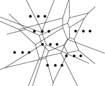
(c) $\operatorname{VD}^{2}(P)$

Figure 1: For $P$, a set of planar sites (a) The nearest site Voronoi diagram (b) The farthest site Voronoi diagram (c) The Voronoi diagram of order $2$.

The nearest site Voronoi diagram for $P$, $\operatorname{NVD}(P)$, is obtained by classifying the points in the plane according to their nearest neighbor in $P$. For each site $p\in P$, the open set of points in $\mathbb{R}^{2}$ with $p$ as their unique nearest site in $P$ is called the Voronoi cell of $p$. For any two sites $p,q\in P$, the bisector $B(p,q)$ of $p$ and $q$ is defined as the line containing all points in the plane that are equidistant to $p$ and $q$. The Voronoi edge for $p$, $q$ consists of all points in the plane with $p$ and $q$ as their only two nearest sites. If it exists, the Voronoi edge for $p$ and $q$ is a subset of the bisector $B(p,q)$ of $p$ and $q$. Our general position assumption, and the fact that $n\geq 3$, guarantee that each Voronoi edge is an open line segment or a halfline. Voronoi vertices are the points in the plane that have exactly three nearest sites in $P$. Again by general position, we have that every point in $\mathbb{R}^{2}$ is either a Voronoi vertex, or lies on a Voronoi edge or in a Voronoi cell. The Voronoi vertices and the Voronoi edges form the set of vertices and edges of a plane graph whose faces are the Voronoi cells. This graph is called the nearest site Voronoi diagram for $P$, $\operatorname{NVD}(P)$; see Figure 1(a). It has $O(n)$ vertices, $O(n)$ edges, and $n$ cells.

The farthest site Voronoi diagram for $P$, $\operatorname{FVD}(P)$, is defined analogously. Farthest Voronoi cells, edges, and vertices are obtained by replacing the term “nearest site” by the term “farthest site” in the respective definitions. Again, the farthest Voronoi vertices and edges constitute the vertices and edges of a plane graph, called $\operatorname{FVD}(P)$. As before, it has $O(n)$ vertices and $O(n)$ edges. However, unlike in $\operatorname{NVD}(P)$, in $\operatorname{FVD}(P)$ it is not necessarily the case that all sites in $P$ have a corresponding cell in $\operatorname{FVD}(P)$. Indeed, the sites with non-empty farthest Voronoi cells are exactly the sites on the convex hull of $P$, $\operatorname{conv}(P)$. Furthermore, all cells in $\operatorname{FVD}(P)$ are unbounded. Hence, $\operatorname{FVD}(P)$, considered as a plane graph, is a tree; see Figure 1(b).

Now, for $k\in\{1,\dots,n-1\}$, the Voronoi diagram of order $k$ for $P$ is obtained by classifying the points in the plane into cells, edges, and vertices according to the set of sites in $P$ that achieve the $k$ smallest distances. We denote the Voronoi diagram of order $k$ for $P$ by $\operatorname{VD}^{k}(P)$; see Figure 1(c). Observe that $\operatorname{NVD}(P)=\operatorname{VD}^{1}(P)$ and $\operatorname{FVD}(P)=\operatorname{VD}^{n-1}(P)$. For each set $Q\subset P$ of $k$ sites from $P$, we denote the Voronoi cell of order $k$ for $Q$ by $C^{k}(Q)$. It is known that $\operatorname{VD}^{k}(P)$ is a plane graph of complexity $O(k(n-k))$ [10, 27]. For simplicity, the cell of $p\in P$ in $\operatorname{NVD}(P)$ and $\operatorname{FVD}(P)$ are denoted, respectively, by $C^{1}(p)$ and $C^{n-1}(p)$. We will denote the boundary of a cell $C$ by $\partial C$. We will give more properties of higher-order Voronoi diagrams in Section 5.

3 A Constant Workspace Algorithm for FVDs and NVDs

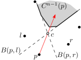
Figure 2: An illustration of Facts 3.1 and 3.2: The sites $l,p,r\in P$ are consecutive on $\operatorname{conv}(P)$. The boundary $\partial C^{n-1}(p)$ contains a subset of $B(p,l)$ and of $B(p,r)$. The ray from $p$ toward $c=B(p,l)\cap B(p,r)$ intersects $\partial C^{n-1}(p)$.

We are given a set $P=\{p_{1},\dots,p_{n}\}$ of $n$ sites in the plane stored in a read-only array to which we have random access. Our task is to report the edges of $\operatorname{NVD}(P)$ and of $\operatorname{FVD}(P)$ using only a constant amount of additional workspace. First, we show how to find a single edge of a given cell of $\operatorname{NVD}(P)$ or of $\operatorname{FVD}(P)$. Then, we repeatedly use this procedure to find all the edges of $\operatorname{NVD}(P)$ and $\operatorname{FVD}(P)$. We summarize the properties of $\operatorname{FVD}(P)$ that are relevant to our algorithms in the following two facts. More details can be found, e.g., in the book by Aurenhammer, Klein, and Lee [10]. See Figure 2 for an illustration.

Fact 3.1.

Let $P$ be a set of $n$ point sites in the plane in general position, and let $p\in P$. The cell $C^{n-1}(p)$ is not empty if and only if $p$ lies on the convex hull of $P$. In this case, the farthest Voronoi cell of $p$ is unbounded. Furthermore, if $r,l\in P$ are the two adjacent sites of $p$ on $\operatorname{conv}(P)$, then $C^{n-1}(p)$ contains an unbounded edge for $p$ and $l$ and an unbounded edge for $p$ and $r$. These edges are subsets of $B(p,l)$ and of $B(p,r)$, respectively.

Fact 3.2.

Let $P$ be a set of $n$ point sites in the plane in general position. Let $l,p,r\in P$ be three consecutive sites on $\operatorname{conv}(P)$, and let $c$ be the intersection of $B(p,l)$ and $B(p,r)$. Then, the ray from $p$ toward $c$ intersects $\partial C^{n-1}(p)$ (not necessarily at $c$).

Lemma 3.3.

Let $P$ be a set of $n$ point sites in the plane in general position. Suppose that $P$ is given in a read-only array. For any $p\in P$, in $O(n)$ time and using constant workspace, we can determine whether $C^{n-1}(p)$ is not empty. If so, we can also find a ray that intersects $\partial C^{n-1}(p)$.

Proof.

By Fact 3.1, it suffices to check whether $p$ lies inside $\operatorname{conv}(P)$. This can be done using simple gift-wrapping: pick an arbitrary site $q\in P\setminus\{p\}$. Scan through $P$ and find the sites $p_{\text{cw}}$ and $p_{\text{ccw}}$ in $P$ which make, respectively, the largest clockwise angle and the largest counterclockwise angle with the ray $pq$, such that both angles are at most $\pi$. Both $p_{\text{cw}}$ and $p_{\text{ccw}}$ are easily obtained in $O(n)$ time using constant workspace. If the cone $p_{\text{cw}}pp_{\text{ccw}}$ that contains $q$ has an opening angle larger than $\pi$, then $p$ is inside $\operatorname{conv}(P)$ and consequently $C^{n-1}(p)$ is empty. Otherwise, $p$ is on $\operatorname{conv}(P)$, with $p_{\text{cw}}$ and $p_{\text{ccw}}$ as its two neighbors. By Fact 3.2, the ray from $p$ through $B(p,p_{\text{cw}})\cap B(p,p_{\text{ccw}})$ intersects $\partial C^{n-1}(p)$. ∎

Lemma 3.4.

Let $P$ be a planar $n$-point set in general position in a read-only array. Suppose we are given a site $p\in P$ and a ray $\gamma$ that emanates from $p$ and intersects $\partial C^{1}(p)$. Then, we can report an edge $e$ of $C^{1}(p)$ that intersects $\gamma$, in $O(n)$ time using $O(1)$ words of workspace. An analogous statement holds for $\operatorname{FVD}(P)$.

Proof.

Among all bisectors $B(p,p^{\prime})$, for $p^{\prime}\in P\setminus\{p\}$, we find a bisector $B^{*}=B(p,p^{*})$ that intersects $\gamma$ closest to $p$. We can find $B^{*}$ by scanning the sites of $P$ and maintaining a closest bisector in each step. The edge $e$ is a subset of $B^{*}$. To find the portion of $B^{*}$ that forms a Voronoi edge in $\operatorname{NVD}(P)$, we do a second scan of $P$. For each $p^{\prime}\in P\setminus\{p,p^{*}\}$, we check where $B(p,p^{\prime})$ intersects $B^{*}$. Each such intersection cuts a piece from $B^{*}$ that cannot appear in $\operatorname{NVD}(P)$, namely the part of $B^{*}$ that is closer to $p^{\prime}$ than to $p$. After scanning all the sites of $P$, the remaining portion of $B^{*}$ is exactly $e$. Since the current piece of $B^{*}$ in each step is connected, we need to store only at most two endpoints in each step. Overall, we can find the edge $e$ of $C^{1}(p)$ that intersects $\gamma$ in $O(n)$ time using $O(1)$ words of workspace.

The procedure for $\operatorname{FVD}(P)$ is analogous, but we take $B^{*}$ to be the bisector intersecting $\gamma$ farthest from $p$, and we cut from $B^{*}$ the pieces that are closer to $p$ than to any other site. ∎

Theorem 3.5.

Suppose we are given a planar $n$-point set $P=\{p_{1},\dots,p_{n}\}$ in general position in a read-only array. We can find all the edges of $\operatorname{NVD}(P)$ in $O(n^{2})$ time using $O(1)$ words of workspace. The same holds for $\operatorname{FVD}(P)$.

Proof.

First, we restate the strategy for $\operatorname{NVD}(P)$ that was proposed by Asano et al. [7], and then we show how to adapt it for $\operatorname{FVD}(P)$.

We go through the sites in $P$. In step $i$, we process $p_{i}\in P$ to detect all edges of $C^{1}(p_{i})$. For this, we need a ray $\gamma$ to apply Lemma 3.4. We choose $\gamma$ as the ray from $p_{i}$ to an arbitrary site of $P\setminus\{p_{i}\}$. This ensures that $\gamma$ intersects $\partial C^{1}(p_{i})$. Now, we use Lemma 3.4 to find an edge $e$ of $C^{1}(p_{i})$ that intersects $\gamma$. We consider the ray $\gamma^{\prime}$ from $p_{i}$ through the left endpoint of $e$ (if it exists), and we apply Lemma 3.4 to find the adjacent edge $e^{\prime}$ of $e$ in $C^{1}(p_{i})$. The ray $\gamma^{\prime}$ hits both $e$ and $e^{\prime}$, so we perform a symbolic perturbation to $\gamma^{\prime}$ so that only $e^{\prime}$ is hit. We repeat this procedure to find further edges of $C^{1}(p_{i})$, in counterclockwise direction. This continues until we return to $e$ or until we find an unbounded edge of $C^{1}(p_{i})$. In the latter case, we start again from the right endpoint of $e$ (if it exists), and we find the remaining edges of $C^{1}(p_{i})$ in clockwise direction.

Since each edge of $\operatorname{NVD}(P)$ is incident to two Voronoi cells, this process will detect each edge twice. To avoid repetitions, whenever we find an edge $e$ of $C^{1}(p_{i})$ with $e\subseteq B(p_{i},p_{j})$, we report $e$ if and only if $i<j$. Since $\operatorname{NVD}(P)$ has $O(n)$ edges, and reporting one edge takes $O(n)$ time and $O(1)$ words of workspace, the result follows.

For $\operatorname{FVD}(P)$, the procedure is almost the same. However, when going through the sites in $P$, for each $p_{i}\in P$, we first check if $C^{n-1}(p_{i})$ is non-empty, using Lemma 3.3. If so, the algorithm from the lemma also gives us a ray $\gamma$ that intersects $\partial C^{n-1}(p_{i})$. From here, we proceed exactly as for $\operatorname{NVD}(P)$ to find the remaining edges of $C^{n-1}(p_{i})$. ∎

4 Obtaining a Time-Space Trade-off

Now we adapt the previous algorithm to a time-space trade-off. Suppose we have $O(s)$ words of workspace at our disposal, for some $s\in\{1,\dots,n\}$. As before, we are given a planar $n$-point set $P=\{p_{1},\dots,p_{n}\}$ in general position in a read-only array, and we would like to report all edges of $\operatorname{NVD}(P)$ or $\operatorname{FVD}(P)$ as quickly as possible. While the algorithm from Section 3 needs two passes over the input to find a single edge of the Voronoi diagram, the idea now is to exploit the additional workspace in order to find $s$ edges of the Voronoi diagram in parallel using two passes. For this, we first show how to find simultaneously a single edge for $s$ different cells of $\operatorname{NVD}(P)$ or of $\operatorname{FVD}(P)$.

Lemma 4.1.

Suppose we are given a set $V=\{v_{1},\dots,v_{s}\}$ of $s$ sites in $P$, and for each $i=1,\dots,s$, a ray $\gamma_{i}$ emanating from $v_{i}$ such that $\gamma_{i}$ intersects the boundary of $C^{1}(v_{i})$. Then, we can report for each $i=1,\dots,s$, an edge $e_{i}$ of $C^{1}(v_{i})$ that intersects $\gamma_{i}$, in $O(n\log s)$ total time using $O(s)$ words of workspace. An analogous statement holds for $\operatorname{FVD}(P)$.

Proof.

The algorithm has two phases. In the first phase, for $i=1,\dots,s$, we find the bisector $B^{*}_{i}$ that contains $e_{i}$, and in the second phase, for $i=1,\dots,s$, we find $e_{i}$, i.e., the portion of $B^{*}_{i}$ that is in $\operatorname{NVD}(P)$.

The first phase proceeds as follows: we group $P$ into batches $Q_{1},Q_{2},\dots,Q_{n/s}$ of $s$ consecutive sites (according to the order in the input array). First, we compute $\operatorname{NVD}(V\cup Q_{1})$. Since $|V\cup Q_{1}|\leq 2s$, this takes $O(s\log s)$ time using $O(s)$ words of workspace. Now, for $i=1,\dots,s$, we find the edge $e_{i}^{\prime}$ of $\operatorname{NVD}(V\cup Q_{1})$ that intersects $\gamma_{i}$ closest to $v_{i}$, and we store the bisector $B_{i}^{\prime}$ that contains $e_{i}^{\prime}$. This can be done in total time $O(|V\cup Q_{1}|)$, since each ray originates in a unique Voronoi cell and since we can simply traverse the whole diagram $\operatorname{NVD}(V\cup Q_{1})$ to find the intersection points. Then, for $j=2,\dots,n/s$, we again compute $\operatorname{NVD}(V\cup Q_{j})$. For $i=1,\dots,s$, we find the edge in $\operatorname{NVD}(V\cup Q_{j})$ that intersects $\gamma_{i}$ closest to $v_{i}$, in total time $O(|V\cup Q_{j}|)$. We update $B_{i}^{\prime}$ to the bisector that contains this edge if and only if its intersection with $\gamma_{i}$ is closer to $v_{i}$ than for the current $B_{i}^{\prime}$. We claim that after all batches $Q_{1},\dots,Q_{n/s}$ have been scanned, $B_{i}^{\prime}$ is the desired bisector $B_{i}^{*}$. To see this, let $B_{i}^{*}=B(v_{i},p)$, for a site $p\in P\setminus\{v_{i}\}$. Then, for the batch $Q_{j}$ with $p\in Q_{j}$, the Voronoi diagram $\operatorname{NVD}(V\cup Q_{j})$ contains an edge on $B_{i}^{*}$. Furthermore, by definition, no other bisector intersects $\gamma_{i}$ closer to $v_{i}$ than $B_{i}^{*}$.

In the second phase, we again group $P$ into batches $Q_{1},\dots,Q_{n/s}$ of size $s$. We again compute $\operatorname{NVD}(V\cup Q_{1})$. For $i=1,\dots,s$, we find the portion of $B_{i}^{*}$ inside the cell of $v_{i}$ in $\operatorname{NVD}(V\cup Q_{1})$, and we store it in $e_{i}$. Then, for $j=2,\dots,n/s$, we compute $\operatorname{NVD}(V\cup Q_{j})$, and for $i=1,\dots,s$, we update the endpoints of $e_{i}$ to the intersection of the current $e_{i}$ and the cell of $v_{i}$ in $\operatorname{NVD}(V\cup Q_{j})$. After processing $Q_{j}$, there is no site in $V\cup\bigcup_{m=1}^{j}Q_{m}$ that is closer to $e_{i}$ than $v_{i}$. Thus, at the end of the second phase, $e_{i}$ is the edge of $C^{1}(v_{i})$ that intersects $\gamma_{i}$. Due to the properties of the Voronoi diagram, throughout the algorithm, $e_{i}$ is a connected subset of $B_{i}^{*}$ (i.e., a ray or a line segment), and it can be described with $O(1)$ words of workspace.

In total, we construct $O(n/s)$ Voronoi diagrams, each with at most $2s$ sites. Since we have $O(s)$ words of workspace available, it takes $O(s\log s)$ time to compute a single Voronoi diagram. Thus, the total running time is $O(n\log s)$. At each point in time, we have $O(s)$ sites in workspace and a constant amount of information for each site, including the Voronoi diagram of these sites, so the space bound is not exceeded. The proof for $\operatorname{FVD}(P)$ is analogous. ∎

Now we describe our time-space trade-off algorithm. At each point in time, we have a set $V$ of $s$ sites in workspace. We use Lemma 4.1 to produce a new edge for each site in $V$. Once all edges for a site $v\in V$ have been found, we discard $v$ from $V$ and replace it with a new site from $P$ (we say that $v$ has been processed completely). We stop this process as soon as all but fewer than $s$ sites have been processed completely. At this point, we do not use Lemma 4.1 any longer. This is because Lemma 4.1 needs two passes of the input to find a single new edge for each site in $V$. Thus, if there is a cell with many edges, too many passes will be necessary. To avoid this, we will need a different method for finding the edges of the remaining cells, see below. We call these remaining cells big, and the other cells small. By definition, all small cells have $O(n/s)$ edges, but big cells may have a lot more edges (even though this does not have to be the case).

In order to avoid doubly reporting edges, our algorithm is split into three phases. In the first phase, we process the whole input to identify the big cells (no edge is reported in this phase). The second phase scans the input again and reports all edges incident to at least one small cell. The third phase reports edges incident to two big cells.

First phase.

The aim of this phase is to find the big cells. We describe how we use Lemma 4.1 in more detail. We scan all sites with non-empty Voronoi cells. For $\operatorname{NVD}(P)$, since all sites have a non-empty cell, we can scan them sequentially. The starting ray is constructed in the same way as in Theorem 3.5. For $\operatorname{FVD}(P)$, by Fact 3.2, we need to find the sites on the convex hull of $P$. For this, we use the algorithm of Darwish and Elmasry [22] that reports the sites on the convex hull of $P$ in clockwise order in $O(\frac{n^{2}}{s\log n}+n\log s)$ time using $O(s)$ words of workspace. We run the Darwish-Elmasry algorithm until $s$ sites on the convex hull have been identified. Then, we suspend the convex hull computation and process those sites. Whenever more sites are needed, we simply resume the convex hull algorithm. Since the convex hull is reported in clockwise order, we know the two neighbors for each site on the convex hull and we can find a starting ray using Fact 3.2

At each point in time, our Voronoi algorithm has $s$ sites from $P$ with non-empty cells in memory. We apply Lemma 4.1 to compute one edge on the cell of each such site. After that, we iteratively update the rays of all sites in memory to find the next edge of each cell, as in Theorem 3.5. Whenever all edges of a cell have been found, we remove the corresponding site from memory, and we replace it with the next relevant site; see Figure 3. Since $(1)$ the Voronoi diagram of $P$ has $O(n)$ edges, $(2)$ in each iteration we produce $s$ edges, and $(3)$ each edge is produced at most twice, it follows that after $O(n/s)$ iterations, fewer than $s$ sites remain in memory. All other sites of $P$ must have been processed.

Thus, after the first phase, we have identified all big cells (those that have not been processed fully). Since there are at most $s$ of them, we can store the corresponding sites explicitly in a table $\mathcal{B}$. We sort those sites according to their indices, so that membership in $\mathcal{B}$ can be tested in $O(\log s)$ time.

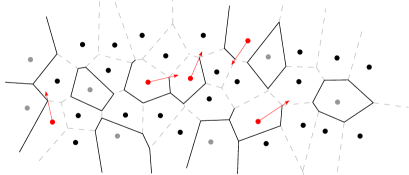
Figure 3: The state of the algorithm at the end of iteration 9 of applying Lemma 4.1, for a set $P$ of $35$ sites and workspace of size $O(s)=O(\lfloor\log n\rfloor)$. The black segments are the edges of $\operatorname{NVD}(P)$ that have already been found. The gray and the red sites represent, respectively, the sites which have been fully processed and those which are currently in the workspace.

Second phase.

The second phase is very similar to the first one. Pick $s$ sites to process; repeatedly use Lemma 4.1 to find edges for each site; once all edges of a site $v$ have been found, replace $v$ with the next site; continue until only big cells remain. The main difference now is we report some Voronoi edges (making sure that every edge is reported exactly once). More precisely, suppose that we discover a Voronoi edge $e$ while scanning the cell $C_{i}$ of a site $v_{i}$, and that $e$ is also incident to the cell $C_{j}$ of the site $v_{j}$. Then, we report $e$ only if one of the following conditions holds:

1. both $C_{i}$ and $C_{j}$ are small and $i<j$; or

2. $C_{i}$ is small and $C_{j}$ is big.

Third phase.

The purpose of the third phase is to report every Voronoi edge that is incident to two big cells. For this, we compute the Voronoi diagram of the sites of big cells, in $O(s\log s)$ time. Let $E_{\mathcal{B}}$ denote the set of its edges. The edges of $E_{\mathcal{B}}$ that are also present in the Voronoi diagram of $P$ need to be reported (the edges may need to be truncated).

In order to determine which edges of $E_{\mathcal{B}}$ remain in the diagram, we proceed similarly as in the second scan of Lemma 4.1: in each step, we compute the Voronoi diagram $\mathcal{V}$ of $\mathcal{B}$ and a batch of $s$ sites from $P$. For each edge $e$ of $E_{\mathcal{B}}$, we check whether $e$ is cut off in $\mathcal{V}$. If so, we update the endpoints of $e$ to the intersection of $e$ and the cell for one of the sites defining $e$. After all edges have been checked, we continue with the next batch of $s$ sites from $P$. After processing all the sites of $P$, the remaining $O(s)$ edges in $E_{\mathcal{B}}$ that have not become empty constitute all the edges of the Voronoi diagram of $P$ that are incident to two big cells. In contrast to Lemma 4.1, we report $O(s)$ edges that are not necessarily incident to $s$ different cells.

Theorem 4.2.

Let $P=\{p_{1},\dots,p_{n}\}$ be a planar $n$-point set in general position stored in a read-only array. Let $s$ be a parameter in $\{1,\dots,n\}$. We can report all edges of $\operatorname{NVD}(P)$ in $O((n^{2}/s)\log s)$ time using $O(s)$ words of workspace. An analogous result holds for $\operatorname{FVD}(P)$.

Proof.

Lemma 4.1 guarantees that the edges reported in the second phase are part of $\operatorname{NVD}(P)$. Also, conditions (i) and (ii) ensure that no edge is reported twice. Clearly, if an edge $e\in\operatorname{NVD}(P)$ is incident to two big cells, the same edge (possibly a superset) must be present in $\operatorname{NVD}(\mathcal{B})$. For the reverse inclusion, first note that since $\mathcal{B}\subset P$, an edge incident to two big cells that is not present in $\operatorname{NVD}(\mathcal{B})$ cannot be present in $\operatorname{NVD}(P)$. Furthermore, for each edge $e$ of $\operatorname{NVD}(\mathcal{B})$, we consider all sites of $P$ and we remove only the portions of $e$ that cannot be present in $\operatorname{NVD}(P)$.

Finally, we need to analyze the running time. The most expensive part of the algorithm lies in the $O(n/s)$ invocations of Lemma 4.1 during the first and the second phase. Other than that, creating the table $\mathcal{B}$ needs $O(s\log s)$ time, and we perform $O(n)$ lookups in $\mathcal{B}$, two for each edge of $\operatorname{NVD}(P)$. Each lookup needs $O(\log s)$ time, so $O(n\log s)$ time in total. The third phase does a single scan over the input, and it computes a Voronoi diagram for each batch of $s$ sites, which totally takes $O(n\log s)$ time. Thus, the running time of the algorithm is $O((n^{2}/s)\log s)$.

At each point during the algorithm, we store only $s$ sites that are currently being processed (along with a constant amount of information attached to each such site), the table $\mathcal{B}$ of at most $s$ sites, the batch of $s$ sites being processed (and the associated Voronoi diagram). All of this can be stored using $O(s)$ words of workspace, as claimed.

For $\operatorname{FVD}(P)$, the approach is analogous. The only difference is that now we must also find the convex hull of $P$. With the algorithm of Darwish and Elmasry [22], this takes $O((n^{2}/s)\log s)$ time for $O(s)$ words of workspace, so the asymptotic running time does not increase. ∎

5 Higher-Order Voronoi Diagrams

(a)

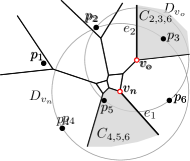
(b)

Figure 4: The diagram $\operatorname{VD}^{k}(P)$ for $k=3$ and $P=\{p_{1},\dots,p_{6}\}$. (a) The interior of the disk $D_{v_{n}}$ with center $v_{n}$ contains $k-1$ sites $\{p_{5},p_{6}\}$, so the $k$-vertex $v_{n}$ is new. The interior of the disk $D_{v_{o}}$ with center $v_{o}$ contains $k-2$ sites $\{p_{3}\}$, so the $k$-vertex $v_{o}$ is old. (b) The $k$-cell $C_{4,5,6}$ is the cell of $\{p_{4},p_{5},p_{6}\}$. The $k$-edge $e_{1}$ is represented by the set $\{p_{5},p_{6}\}$ containing the $k-1$ sites closest to $e_{1}$, the two sites $p_{3}$ and $p_{4}$ that are equidistant to $e_{1}$, and the site $p_{2}$ that defines the $k$-vertex $v_{n}$. Since $v_{n}$ is a new $k$-vertex, the site $p_{2}$ is not among the $k-1$ closest sites to $e_{1}$. The $k$-edge $e_{2}$ of the $k$-cell $C_{2,3,6}$ for $\{p_{2},p_{3},p_{6}\}$ is represented by the set $\{p_{2},p_{3}\}$ of $k-1$ sites closest to $e_{2}$, the two sites $p_{5}$ and $p_{6}$ that are equidistant to $e_{2}$, and the site $p_{2}$ that defines the $k$-vertex $v_{o}$. Since $v_{o}$ is an old $k$-vertex, the site $p_{2}$ is among the $k-1$ closest sites to $e_{2}$.

We now consider computing higher-order Voronoi diagrams [27]. More precisely, we are given an integer $K\in O(\sqrt{s})$, and we would like to report the family of all higher-order Voronoi diagrams of order $k=1,\dots,K$, where we have $O(s)$ words of workspace at our disposal, for some $s\in\{1,\dots,n\}$. For this, we generalize our approach from the previous section, and we combine it with a recursive procedure: for $k=1,\dots,K-1$, we compute the edges of $\operatorname{VD}^{k+1}(P)$ by using previously computed edges of $\operatorname{VD}^{k}(P)$. To make efficient use of the available memory, we perform the computation of the diagrams $\operatorname{VD}^{1}(P),\operatorname{VD}^{2}(P),\dots,\operatorname{VD}^{K}(P)$ in a pipelined fashion, so that in each stage, the necessary edges of the previous Voronoi diagrams are at our disposal and the total memory usage remains $O(s)$.

We begin with some more background on higher-order Voronoi diagrams. Let $x\in\mathbb{R}^{2}$ be a point in the plane. The distance order for $x$ is the sequence of sites in $P$ ordered according to their distance from $x$, from closest to farthest. By our general position assumption, there are at most three sites in $P$ with the same distance to $x$. We call a cell $C$ of $\operatorname{VD}^{k}(P)$ a $k$-cell, and we represent it as the set of $k$ sites that are closest to all points in $C$. Similarly, we call a vertex $v$ of $\operatorname{VD}^{k}(P)$ a $k$-vertex. It is known that there exists a disk $D_{v}$ with center $v$ such that $|\partial D_{v}\cap P|=3$ and $|\mathring{D}_{v}\cap P|\in\{k-2,k-1\}$, where $\partial D_{v}$ is the boundary and $\mathring{D}_{v}$ is the interior of $D_{v}$. We call $v$ an old vertex if $|\mathring{D}_{v}\cap P|=k-2$, and a new vertex if $|\mathring{D}_{v}\cap P|=k-1$; see Figure 4(a). We represent $v$ by the set $D_{v}\cap P$, marking the sites on $\partial D_{v}$. Finally, the edges of $\operatorname{VD}^{k}(P)$ are called $k$-edges. We represent them in a somewhat unusual manner: each edge of $\operatorname{VD}^{k}(P)$ is split into two directed half-edges, such that the half-edges are oriented in opposing directions and such that each half-edge is associated with the $k$-cell to its left. A half-edge $e$ is represented by $k+3$ sites of $P$: the $k-1$ sites closest to $e$, the two sites that come next in the distance order for the points on $e$ and are equidistant to $e$, and one more site for each endpoint of $e$, to define the corresponding $k$-vertices. For each endpoint $v$ of $e$, there are two cases: if $v$ is an old vertex, the third site defining $v$ is among the $k-1$ sites closest to $e$, and if $v$ is a new vertex, the third site is not among those $k-1$ sites; see Figure 4(b). The order of the endpoints encodes the direction of the half-edge. The half-edge is directed from the tail vertex to the head vertex.

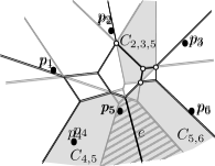
(a)

(b)

Figure 5: The diagrams $\operatorname{VD}^{k}(P)$ (black) and $\operatorname{VD}^{k+1}(P)$ (gray), for $k=2$ and $P=\{p_{1},\dots,p_{6}\}$. (a) The $k$-cells $C_{4,5}=C^{k}(\{p_{4},p_{5}\})$ and $C_{5,6}=C^{k}(\{p_{5},p_{6}\})$ share the $k$-edge $e$. The set $Q=\{p_{4},p_{5}\}\cup\{p_{5},p_{6}\}=\{p_{4},p_{5},p_{6}\}$ gives a non-empty $(k+1)$-cell (shown hashed) which contains $e$. (b) The $(k+1)$-cell $C_{2,3,5}=C^{k+1}(\{p_{2},p_{3},p_{5}\})$ is shown in gray. Inside $C_{2,3,5}$, the edges of $\operatorname{VD}^{k}(P)$ are identical to the edges of $\operatorname{FVD}(\{p_{2},p_{3},p_{5}\})$. These edges meet the boundary of $C_{2,3,5}$ only in the vertices of $C_{2,3,5}$.

We will need several well-known properties of higher-order Voronoi diagrams [27]:

1. let $Q_{1},Q_{2}\subset P$ be two $k$-subsets such that the $k$-cells $C^{k}(Q_{1})$ and $C^{k}(Q_{2})$ are non-empty and adjacent (i.e., share a $k$-edge $e$). Then, the set $Q=Q_{1}\cup Q_{2}$ has size $k+1$, and $C^{k+1}(Q)$ is a non-empty $(k+1)$-cell; see Figure 5(a).

2. Let $Q\subset P$ be a $(k+1)$-subset with $C^{k+1}(Q)$ non-empty. Then, the part of $\operatorname{VD}^{k}(P)$ restricted to $C^{k+1}(Q)$ is identical to (i.e., has the same vertices and edges as) the part of $\operatorname{FVD}(Q)$ restricted to $C^{k+1}(Q)$. Furthermore, the edges of $\operatorname{FVD}(Q)$ in $C^{k+1}(Q)$ do not intersect the boundary, but their endpoints either lie in the interior of $C^{k+1}(Q)$ or coincide with vertices of $C^{k+1}(Q)$. Hence, for every $(k+1)$-cell $C$, the number of $k$-edges in $C$ lies between $1$ and $O(k+1)$, and these edges form a tree; see Figure 5(b).

3. If $v$ is an old $k$-vertex, then it is also a new $(k-1)$-vertex, and if $v$ is a new $k$-vertex, then it is also an old $(k+1)$-vertex. In particular, every vertex appears in exactly two Voronoi diagrams of consecutive order; see Figure 6. Note that all $1$-vertices are new, and all $(n-1)$-vertices are old.

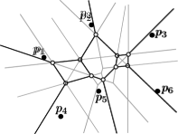
(a)

(b)

Figure 6: The diagram $\operatorname{VD}^{k}(P)$ (black) for $k=2$ and $P=\{p_{1},\dots,p_{6}\}$. (a) The diagram $\operatorname{VD}^{k-1}(P)$ is shown in gray. The empty vertices of $\operatorname{VD}^{k}(P)$ are old $k$-vertices, and they also appear in $\operatorname{VD}^{k-1}(P)$ as new $(k-1)$-vertices. (b) The diagram $\operatorname{VD}^{k+1}(P)$ is shown in gray. The empty vertices of $\operatorname{VD}^{k}(P)$ are new $k$-vertices, and they also appear in $\operatorname{VD}^{k+1}(P)$ as old $(k+1)$-vertices. Every vertex of $\operatorname{VD}^{k}(P)$ appears in exactly one of $\operatorname{VD}^{k-1}(P)$ or $\operatorname{VD}^{k+1}(P)$.

Next, we describe a procedure to generate all (directed) $(k+1)$-half-edges, assuming that we have all (directed) $k$-half-edges at hand. Later, we will combine these procedures, for $k=1,\dots,K$, in a space-efficient manner. Our high-level idea is as follows: let $e$ be a $k$-half-edge. By property (II), the $k$-half-edge $e$ lies inside a $(k+1)$-cell $C$. We will see that we can use $e$ as a starting ray to report all half-edges incident to $C$, similar to Lemma 4.1. However, if we repeat this procedure for every $k$-half-edge, we may report a $(k+1)$-half-edge $\Omega(k)$ times. This will lead to problems when we combine the procedures for computing the Voronoi diagrams of different orders. To avoid this, we do the following: we call a $k$-half-edge relevant if its head vertex lies on the boundary of the $(k+1)$-cell $C$ that contains it. For each $(k+1)$-cell $C$, we partition the boundary of $C$ into intervals of $(k+1)$-half-edges between two consecutive head vertices of relevant $k$-half-edges that lie inside $C$. We assign each such interval to the relevant $k$-half-edge of its clockwise endpoint; see Figures 7(a) and 7(b).

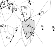
(a)

(b)

(c)

Figure 7: (a) The diagram $\operatorname{VD}^{k}(P)$ (gray) for $k=3$ and $P=\{p_{1},\dots,p_{7}\}$. The $k$-half-edge $e_{1}$ lies in the $(k+1)$-cell $C=C^{k+1}(\{p_{2},p_{3},p_{5},p_{6}\})$. The head vertex of $e_{1}$ is not on $\partial C$, thus $e_{1}$ is not a relevant $k$-half-edge. The opposite direction of $e_{1}$ is also not relevant. (b) The $k$-half-edges $e_{2},e_{3},e_{4},e_{5}$ are relevant, since their head vertices lie on $\partial C$. The interval of $(k+1)$-half-edges on $C$ assigned to each of these $k$-half-edges is shown. In this example, the opposite direction of none of $e_{2},e_{3},e_{4},e_{5}$ is relevant. (c) The $(k+1)$-half-edge $f_{2}$ is incident to the head vertex of $e_{2}$ and lies to the left of the directed line spanned by $e_{2}$. Among all such edges, $f_{2}$ makes the smallest angle $\theta$ with $e_{2}$.

Now, our algorithm goes through all $k$-half-edges. If the current $k$-half-edge $e$ is not relevant, the algorithm does nothing. Otherwise, it reports the $(k+1)$-half-edges of the interval assigned to $e$. This ensures that every half-edge is reported exactly once. As in the previous section, we distinguish between big and small cells in $\operatorname{VD}^{k+1}(P)$, lest we spend too much time on cells with many incident edges. A more detailed description follows below.

The following lemma describes an algorithm that takes $s$ different $k$-half-edges. For each such $k$-half-edge $e$, the algorithm either determines that $e$ is not relevant or finds the first edge of the interval of $(k+1)$-half-edges assigned to $e$.

Lemma 5.1.

Suppose we are given $s$ different $k$-half-edges $e^{k}_{1},\dots,e_{s}^{k}$ represented by the subsets $E_{1},\dots,E_{s}$ of $P$. There is an algorithm that, for $i=1,\dots,s$, either determines that $e_{i}^{k}$ is not relevant, or finds ${e}^{k+1}_{i}$, the first $(k+1)$-edge of the interval assigned to $e_{i}^{k}$. The algorithm takes total expected time $O\big{(}n\log s+nk\,2^{O(\log^{*}k)}\big{)}$ or total deterministic time $O(n\log s+nk\log k)$ and uses $O(sk^{2})$ words of workspace.

Proof.

Our algorithm proceeds analogously to Lemma 4.1. First, we inspect all $k$-half-edges $e_{i}^{k}$. If the head vertex $v$ of $e_{i}^{k}$ is an old $k$-vertex, then $v$ is not a vertex of $\operatorname{VD}^{k+1}(P)$, and it lies in the interior of a $(k+1)$-cell, so $e_{i}^{k}$ is not relevant. Otherwise, $v$ is a new $k$-vertex and an old $(k+1)$-vertex, so it appears on the boundary of a $(k+1)$-cell. In this case, we need to determine the first $(k+1)$-half-edge for the interval assigned to $e_{i}^{k}$. Let $I$ be the set of all indices $i$ such that $e_{i}^{k}$ is relevant.

To determine the first half-edge of each interval, we process the sites in $P$ in batches of size $sk$. In each iteration, we pick a new batch $Q$ of $sk$ sites. Then, we construct $\operatorname{VD}^{k+1}\bigl{(}\bigcup_{i\in I}E_{i}\,\cup\,Q\bigr{)}$ in $O\big{(}sk\log(sk)+sk^{2}\,2^{O(\log^{*}k)}\big{)}$ expected time or in $O(sk\log(sk)+sk^{2}\log k)$ deterministic time (note that $\bigcup_{i\in I}E_{i}\,\cup\,Q$ contains $O(sk)$ sites, so the diagram $\operatorname{VD}^{k+1}\bigl{(}\bigcup_{i\in I}E_{i}\,\cup\,Q\bigr{)}$ has complexity $O(sk^{2})$) [19, 21]. By construction, the head vertex of each $e_{i}^{k}$ with $i\in I$ belongs to the resulting diagram, and we can find each head vertex in $O(\log(sk^{2}))=O(\log(sk))$ time by using a point location structure [14]. Thus, we iterate over all batches, and for each $e^{k}_{i}$, we determine the edge $f^{k+1}_{i}$ that appears in one of the resulting diagrams such that (i) $f^{k+1}_{i}$ is incident to the head vertex of $e^{k}_{i}$; (ii) $f^{k+1}_{i}$ is to the left of the directed line spanned by $e^{k}_{i}$; and (iii) among all such edges, $f^{k+1}_{i}$ makes the smallest angle with $e^{k}_{i}$; see Figure 7(c). We need $O(n/sk)$ iterations to find $f^{k+1}_{i}$. Now, for each $i\in I$, the desired $(k+1)$-half-edge $e^{k+1}_{i}$ is a subset of $f^{k+1}_{i}$. This is because, by property (I) there is one site which is different in the second cell incident to $e^{k+1}_{i}$, and this site exists in one of the batches. Thus, to find the other endpoint of $e_{i}^{k+1}$, as in Lemma 4.1, we perform a second scan over $P$ in batches of $sk$ sites. As before, for each batch $Q$, we construct $\operatorname{VD}^{k+1}\bigl{(}\bigcup_{i\in I}E_{i}\,\cup\,Q\bigr{)}$ and we check, for each $i\in I$, where $f_{i}^{k+1}$ is cut-off in the new diagram. After scanning all the sites of $P$, we have the desired endpoint of $e^{k+1}_{i}$. This is because the endpoint of $e^{k+1}_{i}$ is defined by one more site of $P$, and this site exists in one of the batches. We orient $e_{i}^{k+1}$ such that the cell containing $e_{i}^{k}$ lies to the left of it.

It follows that we can process $s$ edges of $\operatorname{VD}^{k}(P)$ in $O(n/sk)$ iterations, each of which takes $O\big{(}sk\log(sk)+sk^{2}\,2^{O(\log^{*}k)}\big{)}$ expected time or $O(sk\log(sk)+sk^{2}\log k)$ deterministic time. Thus, we get $O\big{(}n\log s+nk\,2^{O(\log^{*}k)}\big{)}$ total expected time or $O(n\log s+nk\log k)$ total deterministic time, using a workspace with $O(sk^{2})$ words (for storing the intermediate Voronoi diagrams). Note that the term $n\log(sk)$ is substituted by $n\log(s)$, since $n\log(sk)=n\log s+n\log k$, and since $n\log k$ is dominated by $nk$ in the total running time. ∎

The algorithm from Lemma 5.1 is actually more general. If, instead of a $k$-half-edge $e_{i}^{k}$ that lies inside a $(k+1)$-cell $C$, we have a $(k+1)$-half-edge $e_{i}^{k+1}$ that lies on the boundary of $C$, the same method of processing $P$ in batches of size $sk$ allows us to find the next $(k+1)$-half-edge incident to $C$ in counterclockwise order from $e_{i}^{k+1}$. These two kinds of edges can be handled simultaneously.

Corollary 5.2.

Let $e_{i}$ denote either a $k$-half-edge or a $(k+1)$-half-edge. Suppose we are given $s$ such half-edges $e_{1},\dots,e_{s}$. Then, we can find in total expected time $O\big{(}n\log s+nk\,2^{O(\log^{*}k)}\big{)}$ or in total deterministic time $O(n\log s+nk\log k)$ and using $O(sk^{2})$ words of workspace a sequence $f_{1},\dots,f_{s}$ of $(k+1)$-half-edges such that, for $i=1,\dots,s$, we have

1. if $e_{i}$ is a relevant $k$-half-edge, then $f_{i}$ is the first $(k+1)$-half-edge of the interval for $e_{i}$;

2. if $e_{i}$ is a $k$-half-edge that is not relevant, then $f_{i}$ is null;

3. if $e_{i}$ is a $(k+1)$-half-edge, then $f_{i}$ is the counterclockwise successor of $e_{i}$.

Lemma 5.3.

Using two scans over all $k$-half-edges, we can report all $(k+1)$-half-edges in batches of size at most $s$ such that each $(k+1)$-half-edge is reported exactly once. This takes $O\bigl{(}\frac{n^{2}k}{s}(\log s+k\,2^{O(\log^{*}k)})\bigr{)}$ expected time or $O\bigl{(}\frac{n^{2}k}{s}(\log s+k\log k)\bigr{)}$ deterministic time using $O(sk^{2})$ words of workspace.

Proof.

The algorithm consists of three phases analogous of the ones introduced in Section 4: in the first phase, we aim at finding the big cells. Let $e_{i}$ denote either a $k$-half-edge or a $(k+1)$-half-edge. To find the big cells we keep $s$ such half-edges $e_{1},\dots,e_{s}$ in memory. At the beginning of this phase, $e_{1},\dots,e_{s}$ are all $k$-half-edges. In each iteration, we apply Corollary 5.2 to these half-edges, to obtain $s$ new $(k+1)$-half-edges $f_{1},\dots,f_{s}$. Now, for each $i=1,\dots,s$, three cases can apply: (i) $f_{i}$ is null, i.e., $e_{i}$ was not relevant. In the next iteration, we replace $e_{i}$ with a fresh $k$-half-edge; (ii)/(iii) $f_{i}$ is not null. Now we need to determine whether $f_{i}$ is the last $(k+1)$-half-edge of its interval. For this, we check whether the head vertex of $f_{i}$ is an old $(k+1)$-vertex. (ii) If $f_{i}$ is not the last $(k+1)$-half-edge of its interval, i.e., if its head vertex is a new $(k+1)$-vertex, we set $e_{i}$ to $f_{i}$ for the next iteration; otherwise, (iii) we set $e_{i}$ to a fresh $k$-half-edge. We repeat this procedure until there are no fresh $k$-half-edges left.

The remaining $(k+1)$-half-edges in the working memory are incident to the big $(k+1)$-cells. For each such cell, we store the center of gravity of its defining sites in an array $\mathcal{B}^{k+1}$, sorted according to lexicographic order. We emphasize that in the first phase, we do not report any $(k+1)$-half-edge.

In the second phase, we repeat the same procedure as in the first phase, but now that we know the big $(k+1)$-cells, we can report edges. In order to avoid repetitions, we only report (i) every $(k+1)$-half-edge incident to a small $(k+1)$-cell; and (ii) the opposite direction of every $(k+1)$-half-edge $e$ incident to a small $(k+1)$-cell, so that the $(k+1)$-cell on the right of $e$ is a big $(k+1)$-cell. We use $\mathcal{B}^{k+1}$ to identify the big cells, by locating the center of gravity of the defining sites of a cell in $\mathcal{B}^{k+1}$ with a binary search, see below for details.

In the third phase, we report every $(k+1)$-half-edge $e$ that is incident to a big $(k+1)$-cell, while the $(k+1)$-cell on the right of $e$ is also a big $(k+1)$-cell. Let $\{\mathcal{B}^{k+1}\}$ denote the sites that define the big $(k+1)$-cells. We construct $\operatorname{VD}^{k+1}(\{\mathcal{B}^{k+1}\})$ in the working memory. Then, we go through the sites in $P$ in batches of size $sk$, adding the sites of each batch to $\operatorname{VD}^{k+1}(\{\mathcal{B}^{k+1}\})$. While doing this, as in the algorithm for Lemma 4.2, we keep track of how the edges of $\operatorname{VD}^{k+1}(\{\mathcal{B}^{k+1}\})$ are cut by the corresponding cell in the new diagrams. In the end, we report all $(k+1)$-edges of $\operatorname{VD}^{k+1}(\{\mathcal{B}^{k+1}\})$ that are not empty. By report, we mean report two $(k+1)$-half-edges in opposing directions. As we explained in the algorithm for Lemma 4.2, these $(k+1)$-half-edges cover all the $(k+1)$-half-edges incident to a big $(k+1)$-cell, while their right cell is also a big $(k+1)$-cell.

Regarding the running time, the first and the second phase consist of $O(nk/s)$ applications of Corollary 5.2 which takes $O\bigl{(}\frac{n^{2}k}{s}(\log s+k\,2^{O(\log^{*}k)})\bigr{)}$ total expected time or $O\bigl{(}\frac{n^{2}k}{s}(\log s+k\log k)\bigr{)}$ total deterministic time. Creating the array $\mathcal{B}^{k+1}$ to represent the big cells takes $O(sk+s\log s)$ steps: we compute the center of gravity of the defining sites for each big $(k+1)$-cell in $O(k)$ steps. Then we sort these center points in lexicographcic order in $O(s\log s)$ steps. A query in $\mathcal{B}^{k+1}$ takes $O(k+\log{s})$ time: given a query $(k+1)$-cell $C$, we compute the center of gravity for its defining sites in $O(k)$ time. Then we use binary-search in $\mathcal{B}^{k+1}$ to find a big $(k+1)$-cell with the same center of gravity. Aurenhammer [9] showed that these centers are pairwise distinct, so that a $(k+1)$-cell can be uniquely identified by the center of gravity of its defining sites.

The algorithm performs at most two queries in $\mathcal{B}^{k+1}$ per $(k+1)$-half-edge, for a total of $O(nk)$ edges. Thus, the total time for the queries is $O(nk^{2}+nk\log s)$. In the third phase, constructing a $(k+1)$-order Voronoi diagram of $O(sk)$ sites takes $O(sk\log s+sk^{2}\,2^{O(\log^{*}k)})$ expected time or $O(sk\log s+sk^{2}\log k)$ deterministic time. We repeat it $O(n/sk)$ times, which takes $O(n\log s+nk\,2^{O(\log^{*}k)})$ expected time or $O(n\log s+nk\log k)$ deterministic time in total.

Overall, the running time of the algorithm simplifies to $O\bigl{(}\frac{n^{2}k}{s}(\log s+k\,2^{O(\log^{*}k)})\bigr{)}$ expected time or $O\bigl{(}\frac{n^{2}k}{s}(\log s+k\log k)\bigr{)}$ deterministic time. The algorithm uses a workspace of $O(sk^{2})$ words, for running Corollary 5.2, for storing big $(k+1)$-cells and for constructing Voronoi diagrams with $O(sk)$ sites. ∎

Now, in order to find the $k$-half-edges for all $k=1,\dots,K$, we proceed as follows: For a parameter $s^{\prime}$ (that we will define later), we compute $s^{\prime}$ different $1$-edges (we report every $1$-edge as two $1$-half-edges in opposing directions). Then, we apply Lemma 5.3 (with parameter $s^{\prime}$) in a pipelined fashion to obtain the $k$-half-edges for $k=2,\dots,K$. In each iteration, the algorithm from Lemma 5.3 consumes at most $s^{\prime}$ different $k$-half-edges from the previous order and produces at most $2s^{\prime}$ new $(k+1)$-half-edges to be used at the next order. This means that if we have between $s^{\prime}$ and $3s^{\prime}$ new $k$-half-edges available in a buffer, then we can use them one by one whenever the algorithm for computing $(k+1)$-half-edges in Lemma 5.3 requires such a new $k$-half-edge. Whenever the size of a buffer falls below $s^{\prime}$, we run the algorithm for the previous order until the buffer size is again between $s^{\prime}$ and $3s^{\prime}$. Applying this idea for all the orders $k=1,\dots,K-1$, we need to store $K-1$ buffers, each containing up to $3s^{\prime}$ half-edges for the corresponding diagram. Since a $k$-half-edge is represented by $O(k)$ sites from $P$, the buffer for $k$-edges requires $O(s^{\prime}k)$ words of workspace. We call this the output buffer and denote it by $\mathcal{O}^{k}$. Furthermore, for each $k$, we need to store $O(s^{\prime})$ half-edges that reflect the current state of the corresponding algorithm. This requires $O(s^{\prime}k)$ words of workspace. This is called the private workspace and is denoted by $\mathcal{P}^{k}$. Finally, for the algorithm that is currently active, we need $O(s^{\prime}k^{2})$ words of workspace to compute the Voronoi diagram of order $k$ for the next batch of $O(s^{\prime}k)$ sites from $P$ (see Lemma 5.3). Since this workspace is used by all the algorithms, it is called the common workspace and denoted by $\mathcal{C}$, see below.

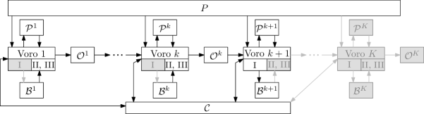
Figure 8: For $k^{\prime}=1,\dots,K$, Voro $k^{\prime}$ is the processor for computing the $k^{\prime}$-half-edges. The roman numerals I, II and III refer to the first, second, and third phase of Voro $k^{\prime}$. The memory cells $\mathcal{P}^{k^{\prime}}$, $\mathcal{O}^{k^{\prime}}$ and $\mathcal{B}^{k^{\prime}}$ indicate the private workspace for Voro $k^{\prime}$, the output buffer for $k^{\prime}$-edges, and the array for big $k^{\prime}$-cells. The common memory of all the processors is called $\mathcal{C}$. The figure shows the algorithm in stage $k$. The direction of the arrows indicates reading from or writing to memory cells. The gray boxes and arrows show the inactive parts in stage $k$. In stage $k$, the algorithm reads data from $\mathcal{B}^{1},\dots,\mathcal{B}^{k}$ and writes into $\mathcal{B}^{k+1}$. In this stage, all the $k$-half-edges are reported and the big $(k+1)$-cells are identified.

Theorem 5.4.

Let $P=\{p_{1},\dots,p_{n}\}$ be a planar $n$-point set in general position, given in a read-only array. Let $s$ be a parameter in $\{1,\dots,n\}$ and $K\in O(\sqrt{s})$. We can report all the edges of $\operatorname{VD}^{1}(P),\dots,\operatorname{VD}^{K}(P)$ in $O\big{(}\frac{n^{2}K^{5}}{s}(\log s+K\,2^{O(\log^{*}K)})\big{)}$ expected time or in $O\big{(}\frac{n^{2}K^{5}}{s}(\log s+K\log K)\big{)}$ deterministic time, using a workspace of size $O(s)$.

Proof.

We compute the half-edges of $\operatorname{VD}^{1}(P),\dots,\operatorname{VD}^{K}(P)$ in a pipelined fashion. The algorithm simulates having $K$ processors, each one computing a Voronoi diagram of different order. For $k=1,\dots,K$, let Voro $k$ be the processor in charge of computing the Voronoi diagram of order $k$. We emphasize that the algorithm is sequential, but the analogy of $K$ processors helps our exposition. Set $s^{\prime}=s/K^{2}$. The first processor Voro $1$ uses the algorithm of Theorem 4.2 with space parameter $s^{\prime}$. For $k\geq 2$, Voro $k$ runs the algorithm from Lemma 5.3 to compute the $k$-half-edges with space parameter $s^{\prime}$. Recall that Lemma 5.3 requires $O(s^{\prime}k^{2})$ words of workspace. This space is needed for computing $\operatorname{VD}^{k}(P)$ for a set of $O(s^{\prime}k)$ sites. However, when Voro $k$ does not compute a diagram, it needs only a state of $O(s^{\prime}k)$ words.

Thus, all the processors share a common workspace $\mathcal{C}$ of size $O(s^{\prime}k)$. At any point in time, $\mathcal{C}$ is used by a single processor Voro $k$ to compute $\operatorname{VD}^{k}(P)$ (for some $k\in\{1,\dots,K\}$). The local state and the other variables needed by each processor Voro $k$ are stored in a private workspace $\mathcal{P}^{k}$. In addition, Voro $k$ has an array $\mathcal{B}^{k}$ to store the big $k$-cells. Whenever an edge of $\operatorname{VD}^{k}(P)$ (for $k\in\{1,\dots,K\}$) would be reported, we instead insert it into an output buffer $\mathcal{O}^{k}$. Each of these local arrays should be able to store $O(s^{\prime})$ half-edges and cells of $\operatorname{VD}^{k}(P)$. Since we need $O(k)$ sites to represent a $k$-half-edge or a $k$-cell, the total space requirement for all processors is $O(s^{\prime}k^{2})=O(s)$.

We simulate the parallel execution of the processors with stages. In stage $0$, we perform only the first phase of Theorem 4.2, to find the $O(s^{\prime})$ big cells of $\operatorname{VD}^{1}(P)$, and we store them in $\mathcal{B}^{1}$. Now, we know the big $1$-cells. Then, in stage $1$, we perform the second and the third phase of Theorem 4.2 to find and report the half-edges of $\operatorname{VD}^{1}(P)$ in batches of size at most $2s^{\prime}$. When we find a batch of $1$-half-edges, we store them in $\mathcal{O}^{1}$. Whenever we have at least $s^{\prime}$ half-edges in $\mathcal{O}^{1}$, we pause Voro $1$, and we start Voro $2$ to perform the first phase of Lemma 5.3 with $\mathcal{O}^{1}$ as input. This gives the half-edges of $\operatorname{VD}^{2}(P)$. Whenever Voro $2$ requires new $1$-half-edges, and the buffer $\mathcal{O}^{1}$ falls below $s^{\prime}$ half-edges, we continue running Voro $1$. When Voro $2$ has consumed all $1$-half-edges and there are less than $s^{\prime}$ half-edges in $\mathcal{P}^{2}$, we stop Voro $2$ (this is the end of the first phase of Lemma 5.3). The current half-edges in $\mathcal{P}^{2}$ represent the big cells of $\operatorname{VD}^{2}(P)$, and we store them in $\mathcal{B}^{2}$. This concludes the description of stage $1$.

In general, in stage $k$ of the algorithm, we have identified the big cells $\mathcal{B}^{1},\dots,\mathcal{B}^{k}$ of the first $k$ diagrams, and we want to use Voro $k+1$ to identify the big cells of $\operatorname{VD}^{k+1}(P)$. For this, we perform the second and the third phase of Theorem 4.2 and Lemma 5.3, for all orders $1,\dots,k$, in a pipelined fashion to generate all half-edges of $\operatorname{VD}^{1}(P),\dots,\operatorname{VD}^{k}(P)$, and we store them in the buffers $\mathcal{O}^{1},\dots,\mathcal{O}^{k}$. We also use $\mathcal{O}^{k}$ as an input of the first phase of Lemma 5.3, which gives us $\mathcal{B}^{k+1}$ for the next stage; see Figure 8. Stage $K$ is similar, but we do not need to determine the big cells of order $K+1$.

By running the $K$ stages of the algorithm, we compute all the Voronoi half-edges and add them to the corresponding output buffers. The edges are computed more than once. Therefore, in order to make sure that they are written into the output memory only once, we report them only the first time they are inserted into the output buffers. For the half-edges of $\operatorname{VD}^{k}(P)$, this happens in stage $k$ of the algorithm. Thus, we can be certain that every half-edge of each diagram $\operatorname{VD}^{1}(P),\dots,\operatorname{VD}^{K}(P)$ is reported exactly once and in order or their containing diagrams (in other words, the $k$-half-edges are reported before the $(k+1)$-half-edges).

Regarding the running time, in each stage $k=1,\dots,K$, we have to compute all diagrams $\operatorname{VD}^{1}(P),\dots,\operatorname{VD}^{k}(P)$, using Lemma 5.3. This takes

$$\sum_{k^{\prime}=1}^{k}O\Big{(}\frac{n^{2}k^{\prime}}{s^{\prime}}\big{(}\log s^{\prime}+k^{\prime}\,2^{O(\log^{*}{k^{\prime}})}\big{)}\Big{)}=O\Big{(}\frac{n^{2}k^{2}}{s^{\prime}}\big{(}\log s^{\prime}+k\,2^{O(\log^{*}k)}\big{)}\Big{)}$$

expected time in stage $k$. The running time for stage $0$ is negligible. The complete algorithm takes

$$\sum_{k=1}^{K}O\Big{(}\frac{n^{2}k^{2}}{s^{\prime}}\big{(}\log s^{\prime}+k\,2^{O(\log^{*}k)}\big{)}\Big{)}=O\Big{(}\frac{n^{2}K^{3}}{s^{\prime}}\big{(}\log s^{\prime}+K\,2^{O(\log^{*}K)}\big{)}\Big{)}$$

expected time for all stages $1$ to $K$. This is $O\Big{(}\frac{n^{2}K^{5}}{s}\big{(}\log s+K\,2^{O(\log^{*}K)}\big{)}\Big{)}$ in terms of $s$, since $s^{\prime}=s/K^{2}$. The analysis for the deterministic running time is completely analogous, replacing the term $2^{O(\log^{*}k)}$ by $\log k$. ∎

Note that our requirement that $K=O(\sqrt{s})$ was crucial in ensuring that the space constraints are not exceeded; we need $\Theta(k)$ words of workspace to store the necessary edges of each $\operatorname{VD}^{k}(P)$, for $k=1,\dots,K-1$, giving a total of $\Theta(K^{2})$ words in our workspace.

6 Conclusion

There are several efficient algorithms that compute a specific higher-order Voronoi diagram without first finding the diagrams of lower order [21, 1, 32]. It would be interesting to extend any of them to obtain a general trade-off, or even an algorithm for constant workspace. For $k=1$ and $k=n-1$, our running times come close to the sorting lower bound which says that the time-space product for sorting is $\Omega(n^{2})$, where the space is measured in bits [15]. Although improvement by a logarithmic factor may be possible, the gap between upper and lower bounds is very small.

There is a much larger gap for general higher-order Voronoi diagrams. We are not aware of any lower bounds (beyond the sorting lower bound). In particular, it would be interesting to have a bound in terms of the order of the diagram (for example, show that $\Omega(n^{2}K^{2}/s)$ steps are needed to find the family of all Voronoi diagrams of order up to $K$ for a given $n$-point set using $s$ words of workspace). Several questions remain also unsolved when looking at upper bounds. Even though we do not believe our algorithms to be optimal, it seems difficult to improve them drastically. Even in constant sized workspaces, we do not know how to improve over the naive running time of $O(n^{4}K)$ that can be obtained by computing the whole arrangement and considering each $k\in\{1,\dots,K\}$ individually.

Acknowledgments.

The authors would like to thank Luis Barba, Kolja Junginger, Elena Khramtcova, and Evanthia Papadopoulou for fruitful discussions on this topic. We would also like to thank the anonymous referees for their thoughtful comments and valuable hints that helped to improve this work.

References

- [1] P. K. Agarwal, M. de Berg, J. Matoušek, and O. Schwarzkopf. Constructing levels in arrangements and higher order Voronoi diagrams. SIAM J. Comput., 27(3):654–667, 1998.
- [2] A. Aggarwal, L. J. Guibas, J. B. Saxe, and P. W. Shor. A linear-time algorithm for computing the Voronoi diagram of a convex polygon. Discrete Comput. Geom., 4:591–604, 1989.
- [3] B. Aronov, M. Korman, S. Pratt, A. van Renssen, and M. Roeloffzen. Time-space trade-offs for triangulating a simple polygon. J. of Comput. Geom., 8(1):105–124, 2017.
- [4] S. Arora and B. Barak. Computational Complexity. A modern approach. Cambridge University Press, 2009.
- [5] T. Asano, K. Buchin, M. Buchin, M. Korman, W. Mulzer, G. Rote, and A. Schulz. Memory-constrained algorithms for simple polygons. Comput. Geom., 46(8):959–969, 2013.
- [6] T. Asano and D. Kirkpatrick. Time-space tradeoffs for all-nearest-larger-neighbors problems. In Proc. 13th Int. Symp. Algorithms Data Structures (WADS), pages 61–72, 2013.
- [7] T. Asano, W. Mulzer, G. Rote, and Y. Wang. Constant-work-space algorithms for geometric problems. J. of Comput. Geom., 2(1):46–68, 2011.
- [8] T. Asano, W. Mulzer, and Y. Wang. Constant-work-space algorithms for shortest paths in trees and simple polygons. J. Graph Algorithms Appl., 15(5):569–586, 2011.
- [9] F. Aurenhammer. A new duality result concerning Voronoi diagrams. Discrete Comput. Geom., 5:243–254, 1990.
- [10] F. Aurenhammer, R. Klein, and D.-T. Lee. Voronoi diagrams and Delaunay triangulations. World Scientific Publishing, 2013.
- [11] Y. Bahoo, B. Banyassady, P. Bose, S. Durocher, and W. Mulzer. Time-space trade-off for finding the -visibility region of a point in a polygon. In Proc. 11th Int. Conf. Alg. Comp. (WALCOM), pages 308–319. Springer-Verlag, 2017.
- [12] L. Barba, M. Korman, S. Langerman, K. Sadakane, and R. I. Silveira. Space–time trade-offs for stack-based algorithms. Algorithmica, 72(4):1097–1129, 2015.
- [13] L. Barba, M. Korman, S. Langerman, and R. I. Silveira. Computing the visibility polygon using few variables. Comput. Geom., 47(9):918–926, 2014.
- [14] M. de Berg, O. Cheong, M. van Kreveld, and M. Overmars. Computational geometry. Algorithms and applications. Springer-Verlag, third edition, 2008.
- [15] A. Borodin and S. A. Cook. A time-space tradeoff for sorting on a general sequential model of computation. SIAM J. Comput., 11:287–297, 1982.
- [16] G. S. Brodal and R. Jacob. Dynamic planar convex hull with optimal query time. In Proc. 7th Scand. Symp. Workshops Algorithm Theory (SWAT), pages 57–70, 2000.
- [17] G. S. Brodal and R. Jacob. Dynamic planar convex hull. In Proc. 43rd Annu. IEEE Symp. Found. Comput. Sci. (FOCS), pages 617–626, 2002.
- [18] H. Brönnimann, T. M. Chan, and E. Y. Chen. Towards in-place geometric algorithms and data structures. In Proc. 20th Annu. Symp. Comput. Geom. (SoCG), pages 239–246, 2004.
- [19] T. M. Chan. Random sampling, halfspace range reporting, and construction of ()-levels in three dimensions. SIAM J. Comput., 30(2):561–575, 2000.
- [20] T. M. Chan and E. Y. Chen. Multi-pass geometric algorithms. Discrete Comput. Geom., 37(1):79–102, 2007.
- [21] T. M. Chan and K. Tsakalidis. Optimal deterministic algorithms for 2-d and 3-d shallow cuttings. Discrete Comput. Geom., 56(4):866–881, 2016.
- [22] O. Darwish and A. Elmasry. Optimal time-space tradeoff for the 2D convex-hull problem. In Proc. 22nd Annu. European Symp. Algorithms (ESA), pages 284–295, 2014.
- [23] A. Elmasry and F. Kammer. Space-efficient plane-sweep algorithms. In Proc. 27th Annu. Internat. Symp. Algorithms Comput. (ISAAC), pages 30:1–30:13, 2016.
- [24] S. Har-Peled. Shortest path in a polygon using sublinear space. J. of Comput. Geom., 7(2):19–45, 2016.
- [25] M. Korman. Memory-constrained algorithms. In Encyclopedia of Algorithms, pages 1260–1264. Springer-Verlag, 2016.
- [26] M. Korman, W. Mulzer, A. van Renssen, M. Roeloffzen, P. Seiferth, and Y. Stein. Time-space trade-offs for triangulations and Voronoi diagrams. In Proc. 14th Int. Symp. Algorithms Data Structures (WADS), pages 482–494, 2015.
- [27] D.-T. Lee. On -nearest neighbor Voronoi diagrams in the plane. IEEE Trans. Computers, 31(6):478–487, 1982.
- [28] J. I. Munro and M. Paterson. Selection and sorting with limited storage. Theoret. Comput. Sci., 12:315–323, 1980.
- [29] J. I. Munro and V. Raman. Selection from read-only memory and sorting with minimum data movement. Theoret. Comput. Sci., 165(2):311–323, 1996.
- [30] J. Pagter and T. Rauhe. Optimal time-space trade-offs for sorting. In Proc. 39th Annu. IEEE Symp. Found. Comput. Sci. (FOCS), pages 264–268, 1998.
- [31] I. Pohl. A minimum storage algorithm for computing the median. Technical Report RC2701, IBM, 1969.
- [32] E. A. Ramos. On range reporting, ray shooting and k-level construction. In Proc. 15th Annu. Symp. Comput. Geom. (SoCG), pages 390–399, 1999.
- [33] J. E. Savage. Models of computation—exploring the power of computing. Addison-Wesley, 1998.