Land Cover Classification from Multi-temporal, Multi-spectral Remotely Sensed Imagery using Patch-Based Recurrent Neural Networks

Abstract

Sustainability of the global environment is dependent on the accurate land cover information over large areas. Even with the increased number of satellite systems and sensors acquiring data with improved spectral, spatial, radiometric and temporal characteristics and the new data distribution policy, most existing land cover datasets were derived from a pixel-based single-date multi-spectral remotely sensed image with low accuracy. To improve the accuracy, the bottleneck is how to develop an accurate and effective image classification technique. By incorporating and utilizing the complete multi-spectral, multi-temporal and spatial information in remote sensing images and considering their inherit spatial and sequential interdependence, we propose a new patch-based RNN (PB-RNN) system tailored for multi-temporal remote sensing data. The system is designed by incorporating distinctive characteristics in multi-temporal remote sensing data. In particular, it uses multi-temporal-spectral-spatial samples and deals with pixels contaminated by clouds/shadow present in the multi-temporal data series. Using a Florida Everglades ecosystem study site covering an area of 771 square kilometers, the proposed PB-RNN system has achieved a significant improvement in the classification accuracy over pixel-based RNN system, pixel-based single-imagery NN system, pixel-based multi-images NN system, patch-based single-imagery NN system and patch-based multi-images NN system. For example, the proposed system achieves 97.21% classification accuracy while a pixel-based single-imagery NN system achieves 64.74%. By utilizing methods like the proposed PB-RNN one, we believe that much more accurate land cover datasets can be produced over large areas efficiently.

I Introduction

Land cover refers to the pattern of ecological resources and human activities dominating different areas of Earth’s surface. It is a critical type of information supporting various environmental science and land management applications at global, regional, and local scales [29, 35]. Given the importance of land cover information in global change and environmental sustainability research, there have been numerous efforts aiming to derive accurate land cover datasets at various scales (e.g, [4, 17, 44, 12, 46, 7]), mostly by using the remote sensing technology. However, even with the increased number of satellite systems and sensors acquiring data with improved spectral, spatial, radiometric and temporal characteristics and the new data distribution policy, most existing land cover datasets were derived from a pixel-based single-date multi-spectral remotely sensed imagery using conventional or advanced pattern recognition techniques such as random forests (RF) [37], neural networks (NNs) [27, 23] and support vector machines (SVM) [47]. The real bottleneck is an accurate and effective image classification technique which can incorporate and utilize the complete multi-spectral, multi-temporal and spatial information available to provide land cover datasets for remote sensing images.

The remote sensing community has been well aware of the relevance of multi-temporal information in land cover mapping, but only limited exploitations have been attempted in actually utilizing such information, mostly from images with much coarse spatial resolutions such as MODIS (Moderate Resolution Imaging Spectroradiometer) time series (e.g.,  [6, 45, 31]). With the recently free availability of several major satellite remotely sensed datasets with much higher spatial resolutions acquired by the Landsat systems, ASTER (Advanced Spaceborne Thermal Emission and Reflection Radiometer), and Sentinels, exploiting multi-temporal information in land cover mapping is becoming more affordable and feasible. However, working with higher-resolution multi-temporal, multi-spectral imagery datasets is facing some crucial challenges mainly caused by the frequent occurrences of pixels contaminated by clouds or shadows  [48] and the incompetency of some conventional pattern recognition methods [7]. Some pixel-based classification efforts attempted to use multiple cloud/shadow-free images acquired at different dates [5, 3]; but they failed to utilize the information of the inherit dependency of multi-temporal remotely sensed data and the invaluable spectral patterns associated with specific classes over time.

This work focuses on exploiting multi-temporal, multi-spectral and spatial information together for improving land cover mapping through the use of RNNs. Recently, RNNs have been demonstrated to achieve significant results on sequential data and have been applied in different fields like natural language processing [30, 34, 20], computer vision [32, 16, 39], multi-modal [22, 11, 15] and robotics [28]. RNNs have been applied on various applications such as language modeling, speech recognition, machine translation, question answering, object recognition, visual tracking, video analysis, image generation, image captioning, video captioning, self driving car, fraud detection, prediction models, sentimental classification, among others. Due to the inherit sequential nature of multi-temporal remote sensing data, such an effective technique could have significant impacts on multi-temporal remote sensing image classification. The remote sensing community has also attempted to utilize RNNs, but most of the existing efforts have been focused on the pixel-based change detection tasks [36, 33, 26], with little on multi-temporal remote sensing image classification. Considering the inherit sequential interdependence of multi-temporal remote sensing data and the spatial relation of a pixel to its neighbourhood, we have developed a patch-based RNN (PB-RNN) system for land cover classification from a Landsat-8 OLI (Operational Land Imager) time series that are freely available from USGS [42]. We targeted medium-resolution Landsat imagery because of their overwhelming use as the primary data for land cover classification and environmental sustainability research. Our proposed method also includes a component to deal with pixels contaminated by clouds/shadow present in the multi-temporal data series. Using a test site in a complicated tropical area in Florida, our proposed PB-RNN system has achieved a significant improvement in the classification accuracy over pixel-based RNN system, pixel-based single-imagery NN system, pixel-based multi-images NN system, patch-based single-imagery NN system and patch-based multi-images NN system.

The remainder of this paper is organized as follows. In Section II, we describe RNNs customized for remote sensing applications. In Section III, we describe our proposed PB-RNN system to map land cover types from multi-temporal, multi-spectral remotely sensed images. In Section IV, we present our experimental results and also compare them with the outcomes from pixel-based RNN system, pixel-based single-imagery NN system, pixel-based multi-images NN system, patch-based single-imagery NN system and patch-based multi-images NN system. Finally, Section V summarizes the major findings and discusses some issues for further research.

II Recurrent Neural Networks (RNNs)

In conventional multilayer NNs, all the inputs belonging to a particular sequence or time series are considered independent to each other and are associated with different parameters present in the network. Due to the above properties, the standard multilayer NNs are limited when dealing with sequential data because these networks are impotent to utilize the inherit dependency between the sequential inputs. On the other hand, RNNs can deal with sequential data efficiently [13]. RNNs consider the dependency between the sequential inputs; and use the same function and same set of parameters at every time step. Using RNN, a sequence of vector x can be processed by applying a recurrence formula at every time step.

$$h_{t}=f(h_{t-1},x_{t};\Theta)$$ (1)

In Equation 1, $h_{t}$ represents the new state which can be obtain using some non-linear function f with old state $h_{t-1}$, input vector $x_{t}$ and set of parameters $\Theta$ as the inputs. In case of simple RNN, the recurrent equations are as follows:

$$h_{t}=f_{h}(W_{x}x_{t}+W_{h}h_{t-1}+b_{h})$$ (2)

$$y_{t}=f_{y}(W_{y}h_{t}+b_{y})$$ (3)

where input, hidden state and output vector of RNN at time t are represented by $x_{t}$, $h_{t}$ and $y_{t}$, respectively, and $W_{x}$, $W_{h}$, $W_{y}$, and $b_{h}$, $b_{y}$ are learnable parameters.
An RNN architecture can be designed in various ways based on their input/output. One-to-sequence, in which a single input is used to generate a sequence as an output for example image captioning [22]. Sequence-to-sequence, where a sequence of data is used to generate a sequence as an output (e.g., machine translation and video classification on frame level) [20, 39]. Sequence-to-one architecture, which takes sequential data as an input to produce a single output (e.g., sentimental classification, automatic movie review) [41]. Land cover classification using our proposed approach to remote sensing imagery bears similar property to the sequence-to-one architecture, where multi-temporal data sequence can be used as an input to classify the desired location into one of the defined classes. Each sample defines a sequence of patches of size $X\times Y\times Z$ labeled using the center pixel, over the time interval of the sequence length; where each datum point in the sequence represents a flatten p-dimensional vector of length p, whose size is $X\times Y\times Z$ at a specific time. However, with the small sequence length, the standard RNN version with non-linear function like sigmoid or hyperbolic tangent works pretty well but the standard version is not capable of dealing with long-term dependencies because of the gradient vanishing and exploding problem while backpropagating in the training stage of RNN. Fortunately, a special kind of RNN named, long short term memory networks (LSTMs) can overcome the gradient vanishing and exploding problem and are capable of dealing with long-term dependencies. The proposed system has also used LSTM to avoid gradient vanishing and exploding problem.

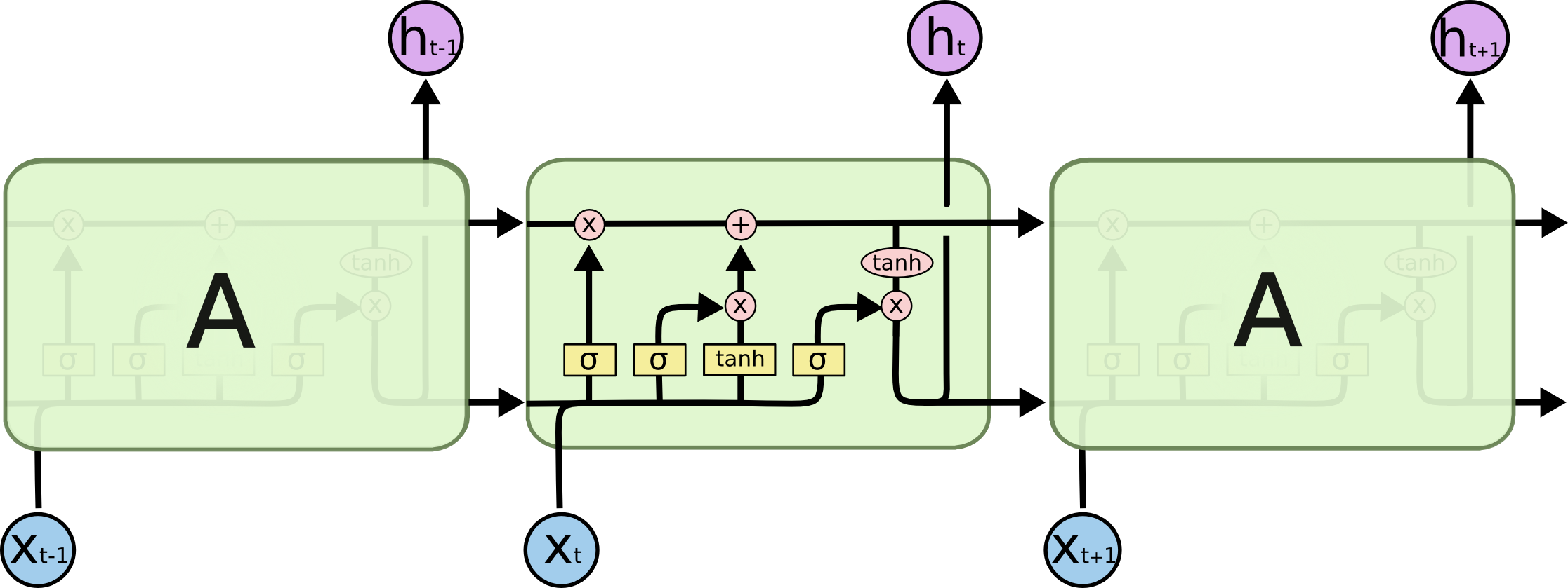
Figure 1: LSTM Architecture

Basically, LSTMs (see Figure 1) work using a gating mechanism with a memory cell. Hidden state is represented as a vector and is calculated using three gates named as input $i$, forget $f$ and output $o$ gates. All of these gates use sigmoid function, which restrict the value of these vectors between 0 and 1. By element-wise multiplying these gates with another vector, these gates define the proportion of other vector they allow to let through. The input gate defines the proportion of newly computed state for the current input it allows to let through. The forget gate controls how much of the previous state it allows to be considered. The output gate decides the proportion of the internal state it passes to the external network. Memory cell $c$ defines the combination of previous memory and the new input. Memory cell $c$ at time $t$ is calculated by combining the element-wise multiplication of the memory cell at previous time point with the forget gate, and the element-wise multiplication of newly computed state with input gate. Finally, LSTM calculates hidden state $h_{t}$ at time $t$ by multiplying the memory cell with the output gate element-wise. The whole architecture can be defined using following equations:

$$i_{t}=sigmoid(W_{x1}x_{t}+W_{h1}h_{t-1})$$ (4)

$$f_{t}=sigmoid(W_{x2}x_{t}+W_{h2}h_{t-1})$$ (5)

$$o_{t}=sigmoid(W_{x3}x_{t}+W_{h3}h_{t-1})$$ (6)

$$g_{t}=tanh(W_{x4}x_{t}+W_{h4}h_{t-1})$$ (7)

$$c_{t}=f_{t}\odot c_{t-1}+i_{t}\odot g_{t}$$ (8)

$$h_{t}=o_{t}\odot tanh(c_{t})$$ (9)

where input, forget and output gates at time $t$ are represented by $i_{t}$, $f_{t}$ and $o_{t}$, respectively; $c_{t}$ represents the cell $c$ at time $t$. Both, current input vector $x_{t}$ at time $t$ and previous hidden state $h_{t-1}$ are used as the inputs in the LSTMs. $W_{x1}$, $W_{x2}$, $W_{x3}$, $W_{x4}$, and $W_{h1}$, $W_{h2}$, $W_{h3}$, $W_{h4}$ are learnable parameters; The element-wise multiplication is denoted by $\odot$ symbol.

These gates with memory cell allow LSTMs to analyze the long dependencies by going deep in time without facing gradient vanishing and exploding problem. Using the input gate, LSTMS are also capable of avoiding cloud/shadow points present in the sequence.

III Proposed Patch-Based RNN System (PB-RNN) for Land Cover Classification

The proposed system is adapted for the land cover classification using complete multi-temporal, multi-spectral and spatial information together for remotely sensed imagery. While the proposed method is generic and should work for all the multi-temporal-spectral remote sensing imagery, we have tested the new method on Landsat images. Below, we define the features used and the architecture adopted.

III-A Multi-Temporal-Spectral Data

Multi-temporal-spectral data are generated in two phases; firstly, we extracted multi-spectral layer stacks out of Landsat images and then a series of layer stacks are combined together to get the final product. In order to convert a Landsat 8 imagery into a multi-spectral layer stack, we have calculated the top-of-atmosphere (TOA) reflectance values associated with the pixels from the scaled digital numbers (DN) belonging to all the OLI bands (except the panchromatic band). TOA reflectance values can be obtained by rescaling and correcting the default 16-bit unsigned integer format DN values using radiometric (reflectance) rescaling coefficients and Sun angle provided in the MTL file present with Landsat 8 product [43]. In the multi-spectral layer stack, each pixel is represented as a vector of length $Z$ consisting TOA reflectance values belonging to $Z$ OLI bands. Landsat 8 program images the entire earth every 16 days; so, if we consider a time series of $N$ images belonging to the desired location then the time interval between any two consecutive images in the series is equal to 16 days. Before generating multi-temporal-spectral data, all the $N$ images in the series are converted into multi-spectral layer stacks explained above, individually. Finally, we club these $N$ multi-spectral layer stacks belonging to a series of $N$ images together.

III-B Multi-Temporal-Spectral-Spatial Samples

In the above mentioned multi-temporal-spectral data, both temporal and spectral information is automatically fused together. However, our proposed system is trying to use the complete multi-spectral, multi-temporal and spatial information available for land cover classification. Therefore, in order to include the spatial information in our samples, we have to extract each sample as a sequence of patches from the above mentioned multi-temporal-spectral data instead of a sequence of $N$ vectors of length $Z$ representing TOA reflectance associated to $Z$ OLI bands belonging to a single pixel. So, each sample is extracted as a sequence of $N$ patches of size $X\times Y\times Z$ labeled using the center pixel where $N$ specifies the sequence length, $X$ the width, $Y$ the height and $Z$ the number of bands, respectively. In this representation, values of the sequence length $N$ and consisting patches of size $X\times Y\times Z$ vary according to the problem and imagery type but the structure of the multi-temporal-spectral-spatial sample remains the same. For the implementation purpose, patches are flattened into vectors of length $X\times Y\times Z$. In the proposed architecture, a series of 23 images are considered and patches of size $3\times 3\times 8$ representing TOA reflectance values of 8 OLI bands (except the panchromatic band) of $3\times 3$ window labeled using the center pixel are flattened into vectors of length 72 (3*3*8). Each sample defines a sequence of 72-dimensional TOA reflectance vectors which consist of spectral and spatial information belonging to the center pixel location of a distinct $3\times 3$ window over the whole year. Each datum point in the sequence represents a TOA reflectance vector at a specific time and there is a time interval of 16 days between any two consecutive points in the sequence; in order to cover the whole year, there are 23 datum points present in the sequence.

III-C Cloud/Shadow Datum Points

In order to deal with cloud/shadow datum points in the sequence, cloud/shadow masks are generated for all the 23 Landsat images using the Fmask Algorithm [48], individually. These masks are then used to locate all the cloud/shadow points present in the multi-spectral layer stacks corresponding to the Landsat images. TOA reflectance vectors of the cloud/shadow locations are set to zero vector. Input gate in the LSTM cell helps to deal cloud/shadow datum vectors by restricting these zero vectors to let through; so that, these cloud/shadow datum points won’t effect the information from the clear datum points.

III-D Training Samples

In order to be consistent with all the other pixel-based and patch-based neural networks used in this paper, image acquired on March 30, 2014 with less than two percent cloud/shadow cover on our test site is used to extract training samples location. In addition, we impose two constraints. First, there should be no cloud/shadow pixel present in the patch at this date. Second, all the boundary patches should be avoided. Eighty percent samples which satisfy the above constraints are extracted separately from all the distinct classes.

III-E Architecture

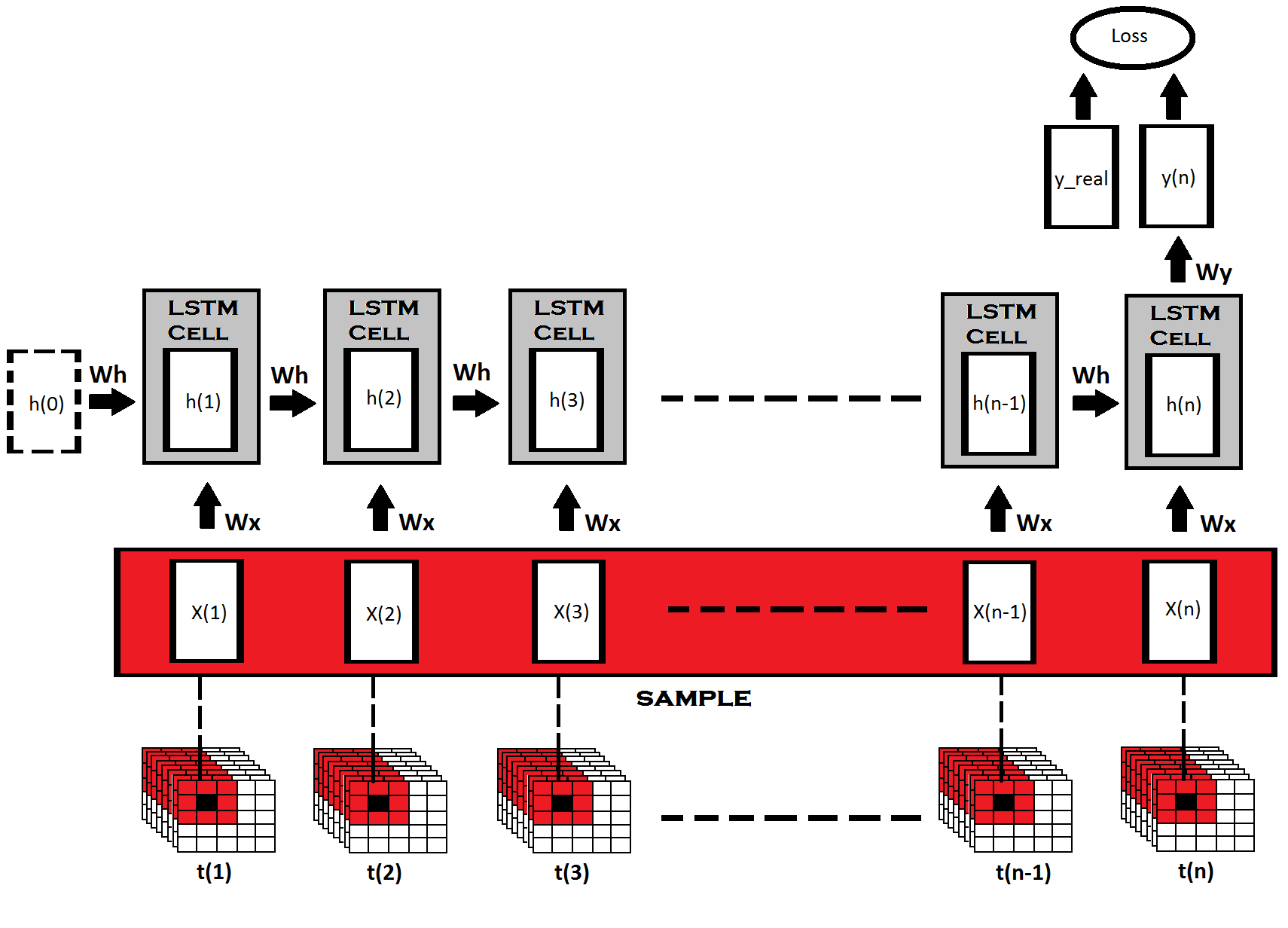
Figure 2: Architecture of the proposed patch-based RNN (PB-RNN) system for land cover classification

Figure 2 illustrates the general overall architecture of the proposed PB-RNN system for land cover classification. Sample X is shown in red; represents a sequence of n vectors ( X(1) to X(n) ) of equal length obtained from time point t(1) to point t(n), respectively. In our experiment, each vector of length 72 (3*3*8) in the sequence is extracted by flattening a patch of size $3\times 3\times 8$ representing TOA reflectance values associated to 8 OLI bands of $3\times 3$ window labeled using the center pixel at a particular time point in the time series and the length of the sequence is 23 to cover the whole year. The softmax layer generates a probability distribution over the eight classes, using the output from the LSTM cell at the 23rd time step as its input.

The proposed system has sequence-to-one architecture, where flattened patch vectors sequence is used as an input to classify the desired location into one of the defined classes. In order to implement this network, we have used Google’s tensorflow (an open source software library for machine intelligence) [1] and Quadro K5200 GPU. The proposed network minimizes the cross entropy using the ADAM optimizer [24] with a learning rate of 0.0001. The ADAM optimizer is a first-order gradient-based optimization algorithm of stochastic objective functions, stochastic gradient descent proves to be a very efficient and effective optimization method in recent deep learning networks (e.g.  [40, 10, 18, 34]).

Using LSTM cell recurrent network, a sequence of vectors X(1:n) can be processed by applying a recurrence formula at every time step. In order to calculate the current hidden state h(t) at time $t$, LSTM cell takes current input vector X(t) from the input sequence and previous hidden state h(t-1) as inputs. Initial hidden state h(0) is initiated as a zero state. Current state depends on all the relevant previous states and input vectors in the sequence; the irrelevant information is controlled by the gate mechanism by resisting it to let through. The proposed system has a fixed length of 23 for the input sequence; so, h(23) is the final hidden state here, and $W_{x}$ and $W_{h}$ are the learnable weight matrices, which remain the same at every time step.

IV Experimental Results and Comparisons

IV-A Test Site

We chose to implement the proposed method on a test site within the Florida Everglades ecosystem; this ecosystem has attracted international attention for the ecological uniqueness and fragility. It is comprised of a wide variety of sub-ecosystems such as freshwater marshes, tropical hardwood hammocks, cypress swamps, and mangrove swamps [9]. Such diverse ecological types make the Everglades an ideal site to test the reliability and robustness of this new system. A series of 23 Landsat8 images was used in our study, where the time interval between any two consecutive images in the series is 16 days. The first image of the series was acquired on February 10, 2014 and the last image on January 28, 2015 (Path 16; Row 42); we extract a subset with a size equivalent to 771 square kilometers ($864\times 991$ pixels) from the whole image as our test site. In order to do single imagery classification, we have used the image acquired on March 30, 2014 with less than two percent cloud/shadow cover on our test site. For multi-images based classification, we have used 4 images acquired on February 10, 2014; March 14, 2014; March 30, 2014; and January 28, 2015 with less than four percent cloud/shadow cover for all of them on our test site.

In order to create a reference map for our research area, we obtained ancillary data from the Florida Cooperative Land Cover Map first and performed correction by comparing it with GPS-guided field observations and the high-resolution images from Google Earth. We have used this reference map to generate training samples and perform accuracy assessments [25]. Using the ancillary data, we adopt a mixed Anderson Level 1/2 land-use/land-cover classification scheme [2] with eight classes (see Table I). Based on our training sample extraction constraints, we are able to generate training samples of size $23\times 72$ for the eight classes, where 23 is the sequence length and 72 (3*3*8) is the flattened patch vector size; the details are shown in Table I.

TABLE I: Land cover classification scheme and training sample size.

No.	Class Name	Description	Training
			Samples
1	High Intensity Urban	Commercial, industrial, institutional constructions with large roofs. Large open spaces and large transportation facilities. Residential areas with impervious surfaces more than half of the total cover.	115879
2	Low Intensity Urban	Residential areas with impervious surfaces less than half of the total cover. Smaller urban service buildings, such as detached stores and restaurants, and state highways.	63726
3	Barren Land	Urban areas with low percentages of constructed materials, vegetation, and low level of impervious surfaces, including bare soil lands, beaches.	14090
4	Forest	Herbaceous cover, trees, trees remain green throughout the year, some wetland evergreen forests included.	90255
5	Cropland	Crops and pastures with vegetation coverage mixed with bushes, small amount fallow land.	77150
6	Woody Wetland	Cypress/tupelo, strand swamp, other coniferous wetland, mixed wetland hardwoods, mangrove swamp.	147851
7	Emergent Herbaceous Wetland	Freshwater non-forested wetland, prairies/bogs, freshwater marshes, wet prairies, saltwater marsh.	39103
8	Water	Streams, canals, lakes, ponds, bays.	116951

IV-B Experimental Results/Comparisons

In this section, we present the experimental results of the proposed PB-RNN system and compare them from those from pixel-based RNN system, pixel-based single-imagery NN system, pixel-based multi-images NN system, patch-based single-imagery NN system and patch-based multi-images NN system. By comparing pixels directly in each of the classification maps from the six different networks for the whole area to the reference map, pixel-based single-imagery NN system achieves accuracy of 62.82%, pixel-based multi-images NN system 63.57%, patch-based single-imagery NN system 73.07%, patch-based multi-images NN system 73.95%, pixel-based RNN system 84.09% and PB-RNN system 96.92%. However, in order to perform quantitative evaluation of the classification results generated by six different neural networks to determine overall and individual category classification accuracy, we have done accuracy assessment using the method described by Congalton [8]. Specifically for each method, an error matrix is generated using the weighted random stratified sampling and then the overall accuracy (OA), Overall kappa (KAPPA), Producer’s accuracy (PA), User’s accuracy (UA) and conditional kappa are calculated based on the error matrix [19].

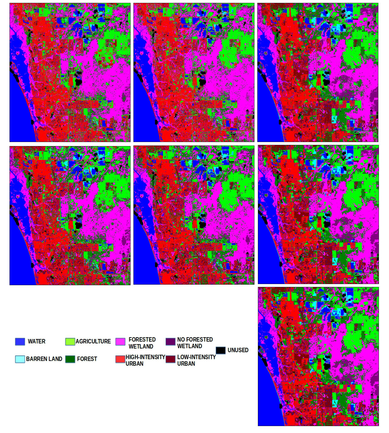
Figure 3: Classification results for the study site from six different methods: (a) Upper Left: Pixel-based single-imagery NN system, (b) Upper Center: Pixel-based multi-images NN system, (c) Upper Right: Pixel-based RNN system, (d) Middle Left: Patch-based single-imagery NN system, (e) Middle Center: Patch-based multi-images NN system, (f) Middle Right: Proposed patch-based RNN (PB-RNN) System and (g) Lower Right: Reference map.

TABLE II: Error Matrix using the Patch-Based RNN (PB-RNN) System.

Classified Data	Reference Data									Accuracy and Conditional Kappa
	High	Low	Barren	Forest	Crop	Woody	Emergent	Water	Row	Producer’s	User’s	Conditional
	Intensity	Intensity	Land		land	Wetland	Herbaceous		Total	Accuracy	Accuracy	Kappa
	Urban	Urban					Wetland			(PA %)	(UA %)
High Intensity Urban	154	2	0	0	1	0	0	1	158	97.47	97.47	0.97
Low Intensity Urban	3	82	0	0	0	1	0	1	87	96.47	94.25	0.94
Barren Land	0	0	50	0	0	0	0	0	50	98.04	100	1.00
Forest	0	0	0	118	1	1	0	0	120	95.93	98.33	0.98
Cropland	0	0	0	1	103	0	1	0	105	98.1	98.1	0.98
Woody Wetland	0	0	0	3	0	195	2	2	202	97.99	96.53	0.96
Emergent Herbaceous	0	0	1	0	0	2	48	0	51	94.12	94.12	0.94
Wetland
Water	1	1	0	1	0	0	0	155	158	97.48	98.1	0.98
Column Total	158	85	51	123	105	199	51	159	931
Overall Accuracy(OA): 97.21%; Overall Kappa(KAPPA): 0.967

TABLE III: Summary of the accuracy assessment for the classification results produced by the new patch-based RNN system (PB-RNN), pixel-based RNN system (Pix RNN), pixel-based single-imagery NN system (Pix Single), pixel-based multi-images NN system (Pix Multi), patch-based single-imagery NN system (Patch Single) and patch-based multi-images NN system (Patch Multi).

Land Cover Class	Conditional Kappa
	Pix Single	Pix Multi	Patch Single	Patch Multi	Pix RNN	PB-RNN	Mean	Standard Deviation
High Intensity Urban	0.54	0.57	0.69	0.71	0.81	0.97	0.72	0.16
Low Intensity Urban	0.54	0.54	0.66	0.67	0.78	0.94	0.69	0.15
Barren Land	0.52	0.66	0.60	0.64	0.85	1.00	0.71	0.18
Forest	0.48	0.53	0.52	0.56	0.79	0.98	0.64	0.20
Cropland	0.57	0.57	0.78	0.78	0.95	0.98	0.77	0.18
Woody Wetland	0.53	0.51	0.69	0.72	0.89	0.96	0.72	0.18
Emergent Herbaceous Wetland	0.57	0.63	0.72	0.83	0.75	0.94	0.74	0.13
Water	0.86	0.88	0.94	0.95	0.94	0.98	0.93	0.05
Mean-Kappa	0.58	0.61	0.70	0.73	0.84	0.97
Standard Deviation	0.12	0.12	0.12	0.12	0.08	0.02
Overall Accuracy(%)	64.74	66.40	75.54	77.63	87.65	97.21
Overall Kappa	0.58	0.60	0.71	0.74	0.86	0.97

TABLE IV: Error Matrix using the Pixel-Based RNN System.

Classified Data	Reference Data									Accuracy and Conditional Kappa
	High	Low	Barren	Forest	Crop	Woody	Emergent	Water	Row	Producer’s	User’s	Conditional
	Intensity	Intensity	Land		land	Wetland	Herbaceous		Total	Accuracy	Accuracy	Kappa
	Urban	Urban					Wetland			(PA %)	(UA %)
High Intensity Urban	137	13	0	4	0	1	0	8	163	91.33	84.05	0.81
Low Intensity Urban	4	69	1	6	1	2	0	3	86	77.53	80.23	0.78
Barren Land	2	1	43	1	2	0	0	1	50	86	86	0.85
Forest	1	1	1	101	5	8	3	3	123	80.16	82.11	0.79
Cropland	1	0	0	1	92	1	0	1	96	90.2	95.83	0.95
Woody Wetland	2	3	1	10	0	186	1	1	204	90.73	91.18	0.89
Emergent Herbaceous	1	1	2	3	1	6	45	0	59	91.84	76.27	0.75
Wetland
Water	2	1	2	0	1	1	0	143	150	89.38	95.33	0.94
Column Total	150	89	50	126	102	205	49	160	931
Overall Accuracy(OA): 87.65%; Overall Kappa(KAPPA): 0.855

The proposed PB-RNN system uses samples, which are in the form of time series of 72-dimensional (3*3*8) flattened TOA reflectance patch vectors of size $23\times 72$. In case of pixel-based RNN system instead of a patch of size $3\times 3\times 8$, each vector in the sequence is representing only the center pixel vector of each patch and this pixel vector is of length 8, containing the TOA reflectance values of 8 OLI bands at that location; so, samples are of size $23\times 8$. Patch-based single-imagery NN system uses 72-dimensional (3*3*8) flattened TOA reflectance patch vectors belonging to patches of size $3\times 3\times 8$ acquired from a single date (March 30, 2014) as samples. On the other hand, pixel-based single-imagery NN system uses only 8-dimensional TOA reflectance center pixel vectors belonging to patches extracted for patch-based single-imagery NN system. In both patch-based and pixel-based multi-images NN system, 72-dimensional (3*3*8) flattened TOA reflectance patch vectors and 8-dimensional TOA reflectance center pixel vectors acquired from four different dates (February 10, 2014; March 14, 2014; March 30, 2014; and January 28, 2015) as samples. The proposed PB-RNN system achieves 97.21% in the overall accuracy and 0.967 in Kappa index. For the individual categories, this new system achieves PA and UA values more than 94% for all classes and the mean of conditional kappa values belonging to 8 different classes (Mean-Kappa) is 0.97 with minimum 0.94 conditional kappa index. In some classes, the system achieves significant improvements. For example barren land, cropland, high intensity urban and woody wetland have (98.04%, 100%, 1.00), (98.1%, 98.1%, 0.98), (97.47%, 97.47%, 0.97) and (97.99%, 96.53%, 0.96) as PA, UA and conditional kappa index values, respectively. The proposed system is able to achieve good results for several spectrally complex classes, such as the low intensity urban and cropland. Table II shows the complete error matrix of system with calculated OA, KAPPA of the overall system and PA, UA, conditional kappa for all individual classes separately.

The proposed PB-RNN system achieves better results than pixel-based RNN system, pixel-based single-imagery NN system, pixel-based multi-images NN system, patch-based single-imagery NN system and patch-based multi-images NN system. Comparative results are summarized in Table III. Figure 3 shows the comparison to reference map from the classification results of six different systems. The proposed system gets 97.21% OA, 0.97 KAPPA, 0.97 Mean-Kappa; which achieves (9.56%, 0.11, 0.13), (19.58%, 0.23, 0.24), (21.76%, 0.26, 0.27), (30.81%, 0.37, 0.36) and (32.47%, 0.39, 0.39) improvements over pixel-based RNN system, patch-based multi-images NN system, patch-based single-imagery NN system, pixel-based multi-images NN system and pixel-based single-imagery NN system, respectively. Table III also shows that there are significant enhancements not only in the overall but also in all the individual categories. Table III shows that the proposed PB-RNN system achieves a minimum 0.15 increase in conditional kappa values for five classes with the maximum 0.19 when comparing with the pixel-based RNN system. In comparison to the patch-based multi-images and single-imagery NN system, the proposed system achieves a minimum 0.20 and 0.22 increase in conditional kappa values for six classes with maximum 0.42 and 0.46 respectively. In case of pixel-based multi-images and single-imagery NN system, the proposed system achieves a minimum 0.31 and 0.37 increase in conditional kappa values for all the classes except water with maximum improvements of 0.45 and 0.50 respectively. The proposed PB-RNN system shows substantial improvements in the conditional kappa results for hard-to-classify classes also. For example, in case of low intensity urban and cropland, there are (0.16, 0.03), (0.27, 0.20), (0.28, 0.20), (0.40, 0.41) and (0.40, 0.41) improvements in conditional kappa values over pixel-based RNN system, patch-based multi-images NN system, patch-based single-imagery NN system, pixel-based multi-images NN system and pixel-based single-imagery NN system, respectively.

Several previous studies have suggested single hidden layer neural networks perform better for classification of remote sensing images [21, 38]. Therefore, we have used only one fully connected hidden layer between input and softmax (outer) layer for both pixel and patch single-imagery NN system; the hidden layer consists of 200 neurons. Patch-based single-imagery NN system uses 72-dimensional (3*3*8) flattened TOA reflectance patch vectors as inputs and pixel-based single-imagery NN system uses only 8-dimensional TOA reflectance center pixel vectors. In case of both multi-images NN systems, we have fused four single-imagery neural network classifiers belonging to different dates together by using joint probabilities of classes at the four dates [5]. Similar to the proposed PB-RNN system, we have used Google’s tensorflow [1] and Quadro K5200 GPU to implement all the other networks also. As shown in Table III and Figure 3, both patch and pixel multi-images NN systems show only slight improvement over their respective single-imagery NN systems in OA, KAPPA, Mean-Kappa of the overall systems and PA, UA, conditional kappa for all individual classes. Unlike the RNN systems, the multi-images NN systems consider each imagery independent to each other and is unable to utilize inherit dependency of multi-temporal remote sensing data. In patch-based multi-images NN system, there is 2.18% improvement in OA, 0.03 improvement in KAPPA, and 0.03 improvement in Mean-Kappa, over patch-based single-imagery NN system. In pixel-based multi-images NN system, there is 1.66% improvement in OA, 0.02 improvement in KAPPA, and 0.03 improvement in Mean-Kappa, comparing to pixel-based single-imagery NN system. Considering spatial information, patch-based single-imagery NN system improves significantly over both pixel-based single-imagery NN system and multi-images NN system. In the patch-based single-imagery NN system, there are 10.71% and 9.05% improvement in OA, 0.13 and 0.11 improvement in KAPPA, and 0.12 and 0.09 improvement in Mean-Kappa, comparing to pixel-based single-imagery NN system and multi-images NN system, respectively. However, without any spatial information the pixel-based RNN system is able to utilize the information of the inherit dependency of multi-temporal remotely sensed data and the invaluable spectral patterns associated with specific classes over time improves significantly over both patch-based NN systems. In pixel-based RNN system, there is 10.02% improvement in OA, 0.12 improvement in KAPPA, and 0.11 improvement in Mean-Kappa, over patch-based multi-images NN system. The same weighted stratified sampling is used for accuracy assessments in all these networks too. The details of the error matrices, OA, KAPPA, PA, UA and and conditional kappa are given in Table IV for pixel-based RNN system, in Table V for pixel-based single-imagery NN system, in Table VI for pixel-based multi-images NN system, in Table VII for patch-based single-imagery NN system and in Table VIII for patch-based multi-images NN system, respectively. The substantial improvements will lead to more accurate land cover data that are essential for many applications (e.g., agriculture monitoring, energy development and resource exploration).

TABLE V: Error Matrix using the Pixel-Based Single-Imagery NN system.

Classified Data	Reference Data									Accuracy and Conditional Kappa
	High	Low	Barren	Forest	Crop	Woody	Emergent	Water	Row	Producer’s	User’s	Conditional
	Intensity	Intensity	Land		land	Wetland	Herbaceous		Total	Accuracy	Accuracy	Kappa
	Urban	Urban					Wetland			(PA %)	(UA %)
High Intensity Urban	130	36	4	8	11	4	4	13	210	76.02	61.90	0.54
Low Intensity Urban	8	29	0	0	6	1	2	4	50	30.85	58	0.54
Barren Land	5	0	27	8	5	1	1	3	50	69.23	54	0.52
Forest	1	3	4	50	9	14	10	1	92	40	54.35	0.48
Cropland	10	10	3	10	71	3	5	3	115	62.28	61.74	0.57
Woody Wetland	6	14	0	43	7	170	23	7	270	83.74	62.96	0.53
Emergent Herbaceous	4	0	0	6	3	5	30	2	50	40	60	0.57
Wetland
Water	7	2	1	0	2	5	0	130	147	79.75	88.44	0.86
Column Total	171	94	39	125	114	203	75	163	984
Overall Accuracy(OA): 64.74%; Overall Kappa(KAPPA): 0.583

TABLE VI: Error Matrix using the Pixel-Based Multi-Images NN system.

Classified Data	Reference Data									Accuracy and Conditional Kappa
	High	Low	Barren	Forest	Crop	Woody	Emergent	Water	Row	Producer’s	User’s	Conditional
	Intensity	Intensity	Land		land	Wetland	Herbaceous		Total	Accuracy	Accuracy	Kappa
	Urban	Urban					Wetland			(PA %)	(UA %)
High Intensity Urban	136	30	6	7	9	2	5	17	212	79.53	64.15	0.57
Low Intensity Urban	7	29	1	2	6	1	1	3	50	36.71	58	0.54
Barren Land	3	1	34	5	5	0	0	2	50	66.67	68	0.66
Forest	3	1	2	46	7	12	7	0	78	35.66	58.97	0.53
Cropland	9	6	5	15	75	8	2	0	120	63.03	62.5	0.57
Woody Wetland	6	10	0	46	12	173	33	5	285	85.22	60.7	0.51
Emergent Herbaceous	1	0	1	7	3	5	33	0	50	40.74	66	0.63
Wetland
Water	6	2	2	1	2	2	0	134	149	83.23	89.93	0.88
Column Total	171	79	51	129	119	203	81	161	994
Overall Accuracy(OA): 66.40%; Overall Kappa(KAPPA): 0.602

TABLE VII: Error Matrix using the Patch-Based Single-Imagery NN system.

Classified Data	Reference Data									Accuracy and Conditional Kappa
	High	Low	Barren	Forest	Crop	Woody	Emergent	Water	Row	Producer’s	User’s	Conditional
	Intensity	Intensity	Land		land	Wetland	Herbaceous		Total	Accuracy	Accuracy	Kappa
	Urban	Urban					Wetland			(PA %)	(UA %)
High Intensity Urban	135	28	3	5	5	3	0	3	182	80.36	74.18	0.69
Low Intensity Urban	12	48	1	2	5	0	0	1	69	51.06	69.57	0.66
Barren Land	4	0	31	4	4	1	2	4	50	70.45	62	0.60
Forest	3	9	2	72	10	15	14	0	125	63.72	57.6	0.52
Cropland	8	3	4	1	86	2	2	1	107	74.14	80.37	0.78
Woody Wetland	4	6	0	27	2	168	13	2	222	84.85	75.68	0.69
Emergent Herbaceous	1	0	0	1	2	8	37	1	50	54.41	74	0.72
Wetland
Water	1	0	3	1	2	1	0	152	160	92.68	95	0.94
Column Total	168	94	44	113	116	198	68	164	965
Overall Accuracy(OA): 75.54%; Overall Kappa(KAPPA): 0.712

TABLE VIII: Error Matrix using the Patch-Based Multi-Images NN system.

Classified Data	Reference Data									Accuracy and Conditional Kappa
	High	Low	Barren	Forest	Crop	Woody	Emergent	Water	Row	Producer’s	User’s	Conditional
	Intensity	Intensity	Land		land	Wetland	Herbaceous		Total	Accuracy	Accuracy	Kappa
	Urban	Urban					Wetland			(PA %)	(UA %)
High Intensity Urban	141	21	4	9	4	2	0	5	186	84.94	75.81	0.71
Low Intensity Urban	10	47	2	2	4	2	1	0	68	64.38	69.12	0.67
Barren Land	3	0	33	4	4	0	2	4	50	71.74	66	0.64
Forest	1	2	4	78	8	21	12	0	126	63.41	61.9	0.56
Cropland	2	1	1	5	89	5	7	1	111	79.46	80.18	0.78
Woody Wetland	4	1	0	21	1	170	19	3	219	84.58	77.63	0.72
Emergent Herbaceous	0	0	1	4	2	1	42	0	50	50.6	84	0.83
Wetland
Water	5	1	1	0	0	0	0	153	160	92.17	95.62	0.95
Column Total	166	73	46	123	112	201	83	166	970
Overall Accuracy(OA): 77.63%; Overall Kappa(KAPPA): 0.737

V Conclusion and future work

In this paper, we have proposed a new patch-based RNN system tailored for land cover classification. The proposed system uses new features to exploit the complete multi-temporal, multi-spectral and spatial information together for land cover mapping. Specifically for Landsat data, we have computed multi-temporal-spectral-spatial samples representing sequence of 23 patches of size $3\times 3\times 8$ belonging to the center pixel location of a distinct $3\times 3$ window over the whole year from multi-temporal-spectral remote sensing imagery. The proposed system is capable of utilizing the spatial information of the inherit dependency of multi-temporal remotely sensed data and the invaluable spectral patterns associated with specific classes over time; by using input gate in the LSTM cell, we are able to deal cloud/shadow pixels by restricting these pixel vectors to let through the input gate. The proposed system is compared to pixel-based RNN system, pixel-based single-imagery NN system, pixel-based multi-images NN system, patch-based single-imagery NN system and patch-based multi-images NN system.. The classification results show that the proposed system achieves significant improvements in both the overall and categorical classification accuracies.

There are further changes that could lead to further improvements. For example, classification accuracy could improve further by creating hierarchical structure classification on the top of the proposed system using different sizes of patches for the same center pixel. Convolution neural network (CNN) can be incorporated with this PB-RNN system to improve the performance even more. We believe that we can develop season-based classifier using the same technique. These and other parameter choices are being investigated further.

References

- [1] Martín Abadi, Ashish Agarwal, Paul Barham, Eugene Brevdo, Zhifeng Chen, Craig Citro, Greg S. Corrado, Andy Davis, Jeffrey Dean, Matthieu Devin, Sanjay Ghemawat, Ian Goodfellow, Andrew Harp, Geoffrey Irving, Michael Isard, Yangqing Jia, Rafal Jozefowicz, Lukasz Kaiser, Manjunath Kudlur, Josh Levenberg, Dan Mané, Rajat Monga, Sherry Moore, Derek Murray, Chris Olah, Mike Schuster, Jonathon Shlens, Benoit Steiner, Ilya Sutskever, Kunal Talwar, Paul Tucker, Vincent Vanhoucke, Vijay Vasudevan, Fernanda Viégas, Oriol Vinyals, Pete Warden, Martin Wattenberg, Martin Wicke, Yuan Yu, and Xiaoqiang Zheng. TensorFlow: Large-scale machine learning on heterogeneous systems, 2015. Software available from tensorflow.org.
- [2] James Richard Anderson. A land use and land cover classification system for use with remote sensor data, volume 964. US Government Printing Office, 1976.
- [3] Damian Bargiel and Sylvia Herrmann. Multi-temporal land-cover classification of agricultural areas in two european regions with high resolution spotlight terrasar-x data. Remote sensing, 3(5):859–877, 2011.
- [4] E. Bartholome and A.S. Belward. Glc2000: a new approach to global land cover mapping from earth observation data. International Journal of Remote Sensing, 26(9), 2005.
- [5] Lorenzo Bruzzone, Diego F Prieto, and Sebastiano B Serpico. A neural-statistical approach to multitemporal and multisource remote-sensing image classification. IEEE Transactions on Geoscience and remote Sensing, 37(3):1350–1359, 1999.
- [6] Hugo Carrão, Paulo Gonçalves, and Mário Caetano. Contribution of multispectral and multitemporal information from modis images to land cover classification. Remote Sensing of Environment, 112(3):986–997, 2008.
- [7] Peng Gong , Jie Wang , Le Yu , Yongchao Zhao , Yuanyuan Zhao , Lu Liang , Zhenguo Niu , Xiaomeng Huang , Haohuan Fu , Shuang Liu , Congcong Li , Xueyan Li , Wei Fu , Caixia Liu , Yue Xu , Xiaoyi Wang , Qu Cheng , Luanyun Hu , Wenbo Yao , Han Zhang , Peng Zhu , Ziying Zhao , Haiying Zhang , Yaomin Zheng , Luyan Ji , Yawen Zhang , Han Chen , An Yan , Jianhong Guo , Liang Yu , Lei Wang , Xiaojun Liu , Tingting Shi , Menghua Zhu , Yanlei Chen , Guangwen Yang , Ping Tang , Bing Xu , Chandra Giri , Nicholas Clinton , Zhiliang Zhu , Jin Chen and Jun Chen. Finer resolution observation and monitoring of global land cover: first mapping results with landsat tm and etm+ data. International Journal of Remote Sensing, 34(7), 2013.
- [8] Russell G Congalton. A review of assessing the accuracy of classifications of remotely sensed data. Remote sensing of environment, 37(1):35–46, 1991.
- [9] Steve Davis and John C Ogden. Everglades: the ecosystem and its restoration. CRC Press, 1994.
- [10] Li Deng, Jinyu Li, Jui-Ting Huang, Kaisheng Yao, Dong Yu, Frank Seide, Michael Seltzer, Geoff Zweig, Xiaodong He, Jason Williams, et al. Recent advances in deep learning for speech research at microsoft. In 2013 IEEE International Conference on Acoustics, Speech and Signal Processing, pages 8604–8608. IEEE, 2013.
- [11] Jeffrey Donahue, Lisa Anne Hendricks, Sergio Guadarrama, Marcus Rohrbach, Subhashini Venugopalan, Kate Saenko, and Trevor Darrell. Long-term recurrent convolutional networks for visual recognition and description. In Proceedings of the IEEE conference on computer vision and pattern recognition, pages 2625–2634, 2015.
- [12] Suming Jin , Limin Yang , Patrick Danielson , Collin Homer , Joyce Fry and George Xian. A comprehensive change detection method for updating the national land cover database to circa 2011. Remote Sensing of Environment, 132(0), 2013.
- [13] Ian Goodfellow, Yoshua Bengio, and Aaron Courville. Deep Learning. MIT Press, 2016.
- [14] Alex Graves, Abdel-rahman Mohamed, and Geoffrey Hinton. Speech recognition with deep recurrent neural networks. In Acoustics, speech and signal processing (icassp), 2013 ieee international conference on, pages 6645–6649. IEEE, 2013.
- [15] Alex Graves, Greg Wayne, and Ivo Danihelka. Neural turing machines. arXiv preprint arXiv:1410.5401, 2014.
- [16] Karol Gregor, Ivo Danihelka, Alex Graves, Danilo Jimenez Rezende, and Daan Wierstra. Draw: A recurrent neural network for image generation. arXiv preprint arXiv:1502.04623, 2015.
- [17] J.A. Fry , G. Xian , S. Jin , J.A. Dewitz , C.G. Homer , L.Yang , C.A. Barnes , N.D. Herold and J.D. Wickham. Completion of the 2006 national land cover database for the conterminous united states. Photogrammetric Engineering and Remote Sensing, 77, 2011.
- [18] Geoffrey E Hinton and Ruslan R Salakhutdinov. Reducing the dimensionality of data with neural networks. Science, 313(5786):504–507, 2006.
- [19] John R. Jensen. Introductory Digital Image Processing: A Remote Sensing Perspective. Pearson Education,Inc., 4th edition, 2015.
- [20] Nal Kalchbrenner and Phil Blunsom. Recurrent continuous translation models. In EMNLP, volume 3, page 413, 2013.
- [21] I Kanellopoulos and GG Wilkinson. Strategies and best practice for neural network image classification. International Journal of Remote Sensing, 18(4):711–725, 1997.
- [22] Andrej Karpathy and Li Fei-Fei. Deep visual-semantic alignments for generating image descriptions. In Proceedings of the IEEE Conference on Computer Vision and Pattern Recognition, pages 3128–3137, 2015.
- [23] T. Kavzoglu and P. M. Mather. The use of backpropagating artificial neural networks in land cover classification. International Journal of Remote Sensing, 24(23), 2003.
- [24] Diederik Kingma and Jimmy Ba. Adam: A method for stochastic optimization. arXiv preprint arXiv:1412.6980, 2014.
- [25] CP Lo and Lee J Watson. The influence of geographic sampling methods on vegetation map accuracy evaluation in a swampy environment. Photogrammetric Engineering and Remote Sensing, 64(12):1189–1200, 1998.
- [26] Haobo Lyu, Hui Lu, and Lichao Mou. Learning a transferable change rule from a recurrent neural network for land cover change detection. Remote Sensing, 8(6):506, 2016.
- [27] J. F. Mas and J. J. Flores. The application of artificial neural networks to the analysis of remotely sensed data. International Journal of Remote Sensing, 29(3), 2008.
- [28] Hongyuan Mei, Mohit Bansal, and Matthew R Walter. Listen, attend, and walk: Neural mapping of navigational instructions to action sequences. arXiv preprint arXiv:1506.04089, 2015.
- [29] William B Meyer and II BL Turner. Changes in land use and land cover: a global perspective, volume 4. Cambridge University Press, 1994.
- [30] Tomas Mikolov, Martin Karafiát, Lukas Burget, Jan Cernockỳ, and Sanjeev Khudanpur. Recurrent neural network based language model. In Interspeech, volume 2, page 3, 2010.
- [31] Ingmar Nitze, Brian Barrett, and Fiona Cawkwell. Temporal optimisation of image acquisition for land cover classification with random forest and modis time-series. International Journal of Applied Earth Observation and Geoinformation, 34:136–146, 2015.
- [32] Pedro Pinheiro and Ronan Collobert. Recurrent convolutional neural networks for scene labeling. In International Conference on Machine Learning, pages 82–90, 2014.
- [33] Bo Qu, Xuelong Li, Dacheng Tao, and Xiaoqiang Lu. Deep semantic understanding of high resolution remote sensing image. In Computer, Information and Telecommunication Systems (CITS), 2016 International Conference on, pages 1–5. IEEE, 2016.
- [34] Geoffrey Hinton, Li Deng , Dong Yu , George E Dahl , Abdel rahman Mohamed , Navdeep Jaitly , Andrew Senior , Vincent Vanhoucke , Patrick Nguyen , Tara N Sainath et al. Deep neural networks for acoustic modeling in speech recognition: The shared views of four research groups. IEEE Signal Processing Magazine, 29(6):82–97, 2012.
- [35] Jonathan A. Foley , Ruth DeFries , Gregory P. Asner , Carol Barford , Gordon Bonan , Stephen R. Carpenter , F. Stuart Chapin , Michael T. Coe , Gretchen C. Daily , Holly K. Gibbs , Joseph H. Helkowski ,Tracey Holloway , Erica A. Howard , Christopher J. Kucharik , Chad Monfreda , Jonathan A. Patz , I. Colin Prentice , Navin Ramankutty and Peter K. Snyder. Global consequences of land use. Science, 309(5734), 2005.
- [36] Tobias Sauter, Björn Weitzenkamp, and Christoph Schneider. Spatio-temporal prediction of snow cover in the black forest mountain range using remote sensing and a recurrent neural network. International Journal of Climatology, 30(15):2330–2341, 2010.
- [37] Di Shi and Xiaojun Yang. An assessment of algorithmic parameters affecting image classification accuracy by random forests. Photogrammetric Engineering & Remote Sensing, 82(6):407–417, 2016.
- [38] Scott M Shupe and Stuart E Marsh. Cover-and density-based vegetation classifications of the sonoran desert using landsat tm and ers-1 sar imagery. Remote Sensing of Environment, 93(1):131–149, 2004.
- [39] Nitish Srivastava, Elman Mansimov, and Ruslan Salakhudinov. Unsupervised learning of video representations using lstms. In International Conference on Machine Learning, pages 843–852, 2015.
- [40] Alex Krizhevsky , Ilya Sutskever and Geoffrey E. Hinton. Imagenet classification with deep convolutional neural networks. In Advances in Neural Information Processing Systems 25. Curran Associates, Inc., 2012.
- [41] Duyu Tang, Bing Qin, and Ting Liu. Document modeling with gated recurrent neural network for sentiment classification. In EMNLP, pages 1422–1432, 2015.
- [42] USGS. Landsat Data Access. http://landsat.usgs.gov/Landsat_Search_and_Download.php, 2016. [Online; accessed 11-Aug-2016].
- [43] USGS. Using the USGS Landsat 8 Product. http://landsat.usgs.gov/Landsat8_Using_Product.php, 2016. [Online; accessed 11-Aug-2016].
- [44] C. Homer , J. Dewitz , J. Fry , M. Coan , N. Hossain , C. Larson , N. Herold , A. McKerrow , J. N. VanDriel and J. Wickham. Completion of the 2001 national land cover database for the conterminous united states. Photogrammetric Engineering and Remote Sensing, 73, 2001.
- [45] Elodie Vintrou, Annie Desbrosse, Agnès Bégué, Sibiry Traoré, Christian Baron, and Danny Lo Seen. Crop area mapping in west africa using landscape stratification of modis time series and comparison with existing global land products. International Journal of Applied Earth Observation and Geoinformation, 14(1):83–93, 2012.
- [46] James E. Vogelmann , Stephen M. Howard , Limin Yang , Charles R. Larson , Bruce K. Wylie and Nicholas J. Van Driel. Completion of the 1990s national land cover data set for the conterminous united states from landsat thematic mapper data and ancillary data sources. Photogrammetric Engineering and Remote Sensing, 67(6), 2001.
- [47] Xiaojun Yang. Parameterizing support vector machines for land cover classification. Photogrammetric Engineering & Remote Sensing, 77(1):27–37, 2011.
- [48] Zhe Zhu and Curtis E. Woodcock. Object-based cloud and cloud shadow detection in landsat imagery. Remote Sensing of Environment, 118, 2012.