Abstract

Let $({\mathcal{M}},\rho)$ be a metric space and let $Y$ be a Banach space. Given a positive integer $m$, let $F$ be a set-valued mapping from ${\mathcal{M}}$ into the family of all compact convex subsets of $Y$ of dimension at most $m$. In this paper we prove a finiteness principle for the existence of a Lipschitz selection of $F$ with the sharp value of the finiteness number.

1. Introduction.

1.1. Main definitions and main results.

Let $({\mathcal{M}},\rho)$ be a pseudometric space, i.e., $\rho:{\mathcal{M}}\times{\mathcal{M}}\to{\mathbb{R}}_{+}\cup\{+\infty\}$ is symmetric, non-negative, satisfies the triangle inequality, and $\rho(x,x)=0$ for all $x\in{\mathcal{M}}$, but $\rho(x,y)$ may be $0$ for $x\neq y$ and $\rho$ may admit the value $+\infty$. We call a pseudometric space $({\mathcal{M}},\rho)$ finite if ${\mathcal{M}}$ is finite, but we say that the pseudometric $\rho$ is finite if $\rho(x,y)$ is finite for every $x,y\in{\mathcal{M}}$.

Let $(Y,\|\cdot\|)$ be a Banach space. Given a non-negative integer $m$ we let ${\mathcal{K}}_{m}(Y)$ denote the family of all non-empty convex compact subsets of $Y$ of dimension at most $m$. We recall that a (single-valued) mapping $f:{\mathcal{M}}\to Y$ is called a selection of a set-valued mapping $F:{\mathcal{M}}\to{\mathcal{K}}_{m}(Y)$ if $f(x)\in F(x)$ for all $x\in{\mathcal{M}}$. A selection $f$ is said to be Lipschitz if there exists a constant $\lambda>0$ such that

$$\|f(x)-f(y)\|\leq\lambda\,\rho(x,y)~{}~{}~{}\text{for all}~{}~{}~{}x,y\in{\mathcal{M}}.$$ (1.1)

We let $\operatorname{Lip}({\mathcal{M}},Y)$ denote the space of all Lipschitz continuous mappings from ${\mathcal{M}}$ into $Y$ equipped with the seminorm $\|f\|_{\operatorname{Lip}({\mathcal{M}},Y)}=\inf\lambda$ where the infimum is taken over all constants $\lambda$ which satisfy (1.1).

Let

$$N(m,Y)=2^{\min\{m+1,\dim Y\}}\,.$$ (1.2)

Our main result is the following “Finiteness Principle for Lipschitz Selections”.

Theorem 1.1

Let $({\mathcal{M}},\rho)$ be a pseudometric space and let $F:{\mathcal{M}}\to{\mathcal{K}}_{m}(Y)$ be a set-valued mapping. Assume that for every subset ${\mathcal{M}}^{\prime}\subset{\mathcal{M}}$ consisting of at most $N(m,Y)$ points, the restriction $F|_{{\mathcal{M}}^{\prime}}$ of $F$ to ${\mathcal{M}}^{\prime}$ has a Lipschitz selection $f_{{\mathcal{M}}^{\prime}}:{\mathcal{M}}^{\prime}\to Y$ whose seminorm satisfies $\|f_{{\mathcal{M}}^{\prime}}\|_{\operatorname{Lip}({\mathcal{M}}^{\prime},Y)}\leq 1$.

Then $F$ has a Lipschitz selection $f:{\mathcal{M}}\to Y$ with $\|f\|_{\operatorname{Lip}({\mathcal{M}},Y)}$ bounded by a constant depending only on $m$.

In Section 6 we prove a variant of this result for finite pseudometric spaces $({\mathcal{M}},\rho)$. We show that in this case the family ${\mathcal{K}}_{m}(Y)$ in the formulation of Theorem 1.1 can be replaced by a wider family $\operatorname{Conv}_{m}(Y)$ of all non-empty convex (not necessarily compact) subsets of $Y$ of dimension at most $m$. See Theorem 6.7.

Before we discuss the main ideas of the proof of Theorem 1.1 let us recall something of the history of the Lipschitz selection problem. The finiteness principle given in this theorem has been conjectured for $Y={\mathbb{R}}^{D}$ in [6], and, in full generality, in [39].

Note that the sharp finiteness number for the case of the trivial distance function $\rho\equiv 0$ is equal to $n(m,Y)=\min\{m+2,\dim Y+1\}$. In fact, the finiteness principle for Lipschitz selections with respect to this trivial pseudometric coincides with the classical Helly’s Theorem [10]: there is a point common to all of the family of sets $\{F(x):x\in{\mathcal{M}}\}\subset{\mathcal{K}}_{m}(Y)$ provided for every $n(m,Y)$-point subset ${\mathcal{M}}^{\prime}\subset{\mathcal{M}}$ the family $\{F(x):x\in{\mathcal{M}}^{\prime}\}$ has a common point. Thus Theorem 1.1 can be considered as a certain generalization of Helly’s Theorem to the case of arbitrary pseudometrics.

For the case $Y={\mathbb{R}}^{2}$ Theorem 1.1 was proved in [39]. Fefferman, Israel and Luli [18] proved this theorem for $({\mathcal{M}},\rho)=({\mathbb{R}}^{n},\|\cdot\|)$ and $Y={\mathbb{R}}^{D}$. An analog of Theorem 1.1 for set-valued mappings into the family $\operatorname{{\it Aff}}_{m}(Y)$ of all affine subspaces of $Y$ of dimension at most $m$ has been proven by Shvartsman in [35] ($Y={\mathbb{R}}^{D}$, see also [37]), [38] ($Y$ is a Hilbert space), and [40] ($Y$ is a Banach space).

The number $N(m,Y)$ from the formulation of Theorem 1.1 is in general sharp.

Theorem 1.2

([37], [39]) Theorem 1.1 is false in general if $N(m,Y)$ is replaced by some number $N$ with $N<N(m,Y)$.

Thus, for every non-negative integer $m$ and every Banach space $Y$ of dimension $\dim Y\geq m$, there exist a metric space $({\mathcal{M}},\rho)$ and a set-valued mapping $F:{\mathcal{M}}\to{\mathcal{K}}_{m}(Y)$ such that the restriction $F|_{{\mathcal{M}}^{\prime}}$ of $F$ to every subset ${\mathcal{M}}^{\prime}\subset{\mathcal{M}}$ consisting of at most $N(m,Y)-1$ points has a Lipschitz selection $f_{{\mathcal{M}}^{\prime}}$ with the seminorm $\|f_{{\mathcal{M}}^{\prime}}\|_{\operatorname{Lip}({\mathcal{M}}^{\prime},Y)}\leq 1$, but nevertheless $F$ does not have a Lipschitz selection.

See also Section 8 where we describe main ideas of the proof of this result for $m=1$ and $m=2$.

1.2. Main ideas of our approach.

Let us briefly indicate the main ideas of the proof of Theorem 1.1.

One of the main ideas in this proof is to bring in the notion of Nagata dimension. The Nagata dimension (or Assouad-Nagata dimension) [26, 1] of a metric space is a certain metric version of the topological dimension. We recall one of the equivalent definitions of this notion. See, e.g., [4].

Definition 1.3

(“Nagata Condition” and “Nagata Dimension”) We say that $(X,d)$ satisfies the Nagata condition if there exist a constant $c_{NC}\in(0,1]$ and a non-negative integer $D_{NC}$ such that for every $s>0$ there exists a cover of $X$ by subsets of diameter at most $s$, at most $D_{NC}+1$ of which meet any given ball in $X$ of radius $c_{NC}s$.

We refer to the smallest value of $D_{NC}$ as the Nagata dimension. More specifically, the Nagata dimension $\dim_{N}X$ of a metric space $(X,d)$ is the smallest integer $n$ for which there exists a constant $C\geq 1$ such that for all $s>0$, there exists a covering of $X$ by subsets of diameter at most $s$ with every ball in $X$ of diameter at most $s/C$ meeting at most $n+1$ elements of the covering.

We refer the reader to [23, 4, 24] and references therein for numerous results related to the Nagata condition and dimension.

Theorem 1.4

Let $(X,d)$ be a finite metric space satisfying the Nagata condition with constants $c_{NC}$, $D_{NC}$. Given $m\in{\mathbb{N}}$ there exist a constant $k^{\sharp}\in{\mathbb{N}}$ depending only on $m$, and a constant $\gamma>0$ depending only on $m$, $c_{NC}$, $D_{NC}$, for which the following holds :

Let $\lambda$ be a positive constant and let $F:X\to\operatorname{Conv}_{m}(Y)$ be a set-valued mapping such that, for every subset $X^{\prime}\subset X$ consisting of at most $k^{\sharp}$ points, the restriction $F|_{X^{\prime}}$ of $F$ to $X^{\prime}$ has a Lipschitz selection $f_{X^{\prime}}:X^{\prime}\to Y$ whose seminorm satisfies $\|f_{X^{\prime}}\|_{\operatorname{Lip}(X^{\prime},Y)}\leq\lambda$.

Then $F$ has a Lipschitz selection $f:X\to Y$ with $\|f\|_{\operatorname{Lip}(X,Y)}\leq\gamma\lambda$.

We consider the proof of Theorem 1.4, which we present in Sections 2-4, to be the most difficult technical part of this paper.

To establish Theorem 1.4 we adapt the proof of a finiteness principle for $C^{m}$ selection [18] from ${\mathbb{R}}^{n}$ to a metric space $X$ of bounded Nagata dimension. As in [18], the geometry of certain convex sets $\Gamma_{\ell}(x)$, $(\ell\geq 0,x\in X)$ plays a crucial role. We refer the reader to the introduction of [18] and the website [19].

In Section 2.1 we consider an important family of metric spaces with finite Nagata dimension - the family of finite metric trees. We recall that a finite metric space $(X,d)$ is said to be a metric tree if $X$ is equipped with a structure of a (graph-theoretic) tree so that for every $x,y\in X$

$$d(x,y)=\sum\limits_{i=0}^{k-1}d(z_{i},z_{i+1})$$

where $\{z_{0},z_{1},...,z_{k}\}$ is the unique “path” in $X$ joining $x$ to $y$ (i.e., $z_{0}=x$, $z_{k}=y$, $z_{i}\neq z_{j}$ for $i\neq j$, and $z_{j}$ joined to $z_{j+1}$ by an edge).

It is proven in [23] that every metric tree satisfies the Nagata condition (with absolute constants $c_{NC},D_{NC}$), and the Nagata dimension of an arbitrary metric tree is $1$. See also Lemma 2.1.

Hence we conclude that Theorem 1.4 is true for every finite metric tree. See Corollary 4.15.

Let

$${\mathcal{K}}(Y)={\bigcup}\,\{{\mathcal{K}}_{m}(Y):m\in{\mathbb{N}}\}$$

be the family of all non-empty finite dimensional convex compact subsets of the Banach space $Y$, and let $\operatorname{d_{H}}$ denote the Hausdorff distance between subsets of $Y$. Basing on Corollary 4.15, in Section 5 we prove the following theorem which actually reduces the original problem to the case of the metric space $({\mathcal{K}}_{m}(Y),\operatorname{d_{H}})$.

Theorem 1.5

Let $({\mathcal{M}},\rho)$ be a metric space. Let $m\geq 1$ and let $F:{\mathcal{M}}\to{\mathcal{K}}_{m}(Y)$ be a set-valued mapping. Suppose that for every subset ${\mathcal{M}}^{\prime}\subset{\mathcal{M}}$ consisting of at most $k^{\sharp}$ points, the restriction $F|_{{\mathcal{M}}^{\prime}}$ of $F$ to ${\mathcal{M}}^{\prime}$ has a Lipschitz selection $f_{{\mathcal{M}}^{\prime}}:{\mathcal{M}}^{\prime}\to Y$ whose seminorm satisfies $\|f_{{\mathcal{M}}^{\prime}}\|_{\operatorname{Lip}({\mathcal{M}}^{\prime},Y)}\leq 1$.

Then there exists a mapping $G:{\mathcal{M}}\to{\mathcal{K}}_{m}(Y)$ satisfying the following conditions:

(i). $G(x)\subset F(x)$ for every $x\in{\mathcal{M}}$;

(ii). For every $x,y\in{\mathcal{M}}$ the following inequality

$$\operatorname{d_{H}}(G(x),G(y))\leq\gamma_{0}\,\rho(x,y)$$

holds. Here $\gamma_{0}$ is a constant depending only on $m$, and $k^{\sharp}=k^{\sharp}(m)$ is the constant from Theorem 1.4.

At the next step of the proof of Theorem 1.1 we apply to the mapping $G$ the following Lipschitz selection theorem for the metric space $({\mathcal{K}}(Y),\operatorname{d_{H}})$.

Theorem 1.6

([39]) There exists a mapping $S_{Y}:{\mathcal{K}}(Y)\to Y$ such that

(i). $S_{Y}(K)\in K$ for each $K\in{\mathcal{K}}(Y)$;

(ii). For every $K_{1},K_{2}\in{\mathcal{K}}(Y)$,

$$\|S_{Y}(K_{1})-S_{Y}(K_{2})\|\leq\gamma_{1}\operatorname{d_{H}}(K_{1},K_{2})$$

where $\gamma_{1}=\gamma_{1}(\dim K_{1},\dim K_{2})$ is a constant depending only on dimensions of $K_{1}$ and $K_{2}$.

We refer to $S_{Y}(K)$ as a Steiner-type point of a convex set $K\in{\mathcal{K}}(Y)$. See Section 7 for more detail.

Finally, we put

$$f(x)=S_{Y}(G(x)),~{}~{}~{}x\in{\mathcal{M}},$$

where $G:{\mathcal{M}}\to{\mathcal{K}}_{m}(Y)$ is the set-valued mapping from Theorem 1.5.

Clearly, by part (i) of Theorem 1.6 and part (i) of Theorem 1.5,

$$f(x)=S_{Y}(G(x))\in G(x)\subset F(x)~{}~{}~{}\text{for all}~{}~{}~{}x\in{\mathcal{M}},$$

proving that the function $f:{\mathcal{M}}\to Y$ is a selection of $F$. In turn, by part (ii) of Theorem 1.6 and part (ii) of Theorem 1.5, for every $x,y\in{\mathcal{M}}$

$$\|f(x)-f(y)\|=\|S_{Y}(G(x))-S_{Y}(G(y))\|\leq\gamma_{1}\,\operatorname{d_{H}}(G(x),G(y))\leq\gamma_{0}\,\gamma_{1}\,\rho(x,y).$$

Here $\gamma_{1}$ is a constant depending only on $\dim G(x)$ and $\dim G(y)$. Since $\dim G(x),\dim G(y)\leq m$, and $\gamma_{0}$ depends only on $m$, the Lipschitz seminorm of $f$ on ${\mathcal{M}}$ is bounded by a constant depending only on $m$.

This proves a version of Theorem 1.1 with $N(m,Y)$ replaced by $k^{\sharp}$ for an arbitrary metric space $({\mathcal{M}},\rho)$. See Corollary 5.12.

Using this result, in Section 6 we prove a similar version of Theorem 1.1 for the general case, i.e., for an arbitrary pseudometric space $({\mathcal{M}},\rho)$. See Proposition 6.1.

Finally, using Theorem 1.7 below, we obtain the statement of Theorem 1.1 in its original form.

Theorem 1.7

Let $({\mathcal{M}},\rho)$ be a finite pseudometric space with a finite pseudometric $\rho$, and let ${F:{\mathcal{M}}\to\operatorname{Conv}_{m}(Y)}$ be a set-valued mapping. Suppose that for every subset ${\mathcal{M}}^{\prime}\subset{\mathcal{M}}$ with $\#{\mathcal{M}}^{\prime}\leq N(m,Y)$ the restriction $F|_{{\mathcal{M}}^{\prime}}$ has a Lipschitz selection $f_{{\mathcal{M}}^{\prime}}:{\mathcal{M}}^{\prime}\to Y$ with $\|f_{{\mathcal{M}}^{\prime}}\|_{\operatorname{Lip}({\mathcal{M}}^{\prime},Y)}\leq 1$.

Then $F$ has a Lipschitz selection $f:{\mathcal{M}}\to Y$ with $\|f\|_{\operatorname{Lip}({\mathcal{M}},Y)}\leq\gamma$ where $\gamma$ is a positive constant depending only on $m$ and $\#{\mathcal{M}}$.

(Recall that $\operatorname{Conv}_{m}(Y)$ denotes the family of all non-empty convex subsets of $Y$ of dimension at most $m$.)

We prove Theorem 1.7 in Section 6. This result enables us to replace the finiteness number $k^{\sharp}$ by the required sharp finiteness number $N(m,Y)$, completing the proof of Theorem 1.1.

In Section 8 we present various remarks and comments related to the sharp finiteness principle proven in Theorem 1.1.

The existence of Lipschitz selections is closely related to Whitney’s Extension Problem [44]:

Fix $m,n\geq 1$. Given $E\subset{\mathbb{R}}^{n}$ and $\varphi:E\to{\mathbb{R}}$, decide whether $\varphi$ extends to a $C^{m}$ function $f:{\mathbb{R}}^{n}\to{\mathbb{R}}$. If such an extension exists, then how small can we take its $C^{m}$-norm?

There is a finiteness theorem for such problems and their relatives; see Brudnyi-Shvartsman [6, 7, 8, 36, 39, 41] and later papers by Fefferman, Klartag, Israel, Luli [11, 12, 13, 14, 15, 16, 17, 18, 20]. See also A. Brudnyi, Yu. Brudnyi [5].

In Brudnyi-Shvartsman [7, 8, 36, 39, 41], Lipschitz selection served as the main tool to attack Whitney’s Problem. The later work [11, 12, 13, 14, 15, 16, 18, 20] made no explicit mention of Lipschitz selection, but broadened Whitney’s Problem to study $C^{m}$ functions $f:{\mathbb{R}}^{n}\to{\mathbb{R}}$ that agree only approximately with a given function $\varphi$ on $E$.

A Lipschitz selection problem can obviously be viewed as a search for a Lipschitz mapping $f:{\mathcal{M}}\to Y$ that agrees approximately with data.

As in [18], our present results lead to questions about efficient computation for Lipschitz selection problems on finite metric spaces. In connection with such issues, we ask whether the results of Har-Peled and Mendel [22] on the Well Separated Pairs Decomposition [9] can be extended from doubling metrics to metrics of bounded Nagata dimension.

Acknowledgments. We are grateful to Alexander Brudnyi, Arie Israel, Bo’az Klartag, Garving (Kevin) Luli and the participants of the 10th Whitney Problems Conference, Williamsburg, VA, for valuable conversations.

We are grateful also to the College of William and Mary, Williamsburg, VA, USA, the American Institute of Mathematics, San Jose, CA, USA, the Fields Institute, Toronto, Canada, the Banff International Research Station, Banff, Canada, the Centre International de Rencontres Mathématiques (CIRM), Luminy, Marseille, France, and the Technion, Haifa, Israel, for hosting and supporting workshops on the topic of this paper and closely related problems.

Finally, we thank the US-Israel Binational Science Foundation, the US National Science Foundation, the Office of Naval Research and the Air Force Office of Scientific Research for generous support.

2. Nagata dimension and Whitney partitions on metric trees.

2.1. Metric trees and Nagata condition.

Let $(X,d)$ be a metric space. We write $B(x,r)$ to denote the ball $\{y\in X:d(x,y)<r\}$ (strict inequality) in the metric space $(X,d)$. We also write $\operatorname{diam}A=\sup\,\{d(a,b):a,b\in A\}$ and

$$\operatorname{dist}(A^{\prime},A^{\prime\prime})=\inf\{d(a^{\prime},a^{\prime\prime}):a^{\prime}\in A^{\prime},a^{\prime\prime}\in A^{\prime\prime}\}$$

to denote the diameter of a set $A\subset X$ and the distance between sets $A^{\prime},A^{\prime\prime}\subset X$ respectively.

Let us consider an important example of a metric space with finite Nagata dimension.

Let $T=(X,E)$ be a finite tree. Here $X$ denotes the set of nodes and $E$ denotes the set of edges of $T$. We write $x\leftrightarrow y$ to indicate that nodes $x,y\in X$, $x\neq y$, are joined by an edge; we denote that edge by $[xy]$.

Suppose we assign a positive number $\Delta(e)$ to each edge $e\in E$. Then we obtain a notion of distance $d(x,y)$ for any $x,y\in X$, as follows.

We set

$$d(x,x)=0~{}~{}~{}\text{for every}~{}~{}~{}x\in X.$$ (2.1)

Because $T$ is a tree, any two distinct nodes $x,y\in X$ are joined by one and only “path”

$$x=x_{0}\leftrightarrow x_{1}\leftrightarrow...\leftrightarrow x_{L}=y~{}~{}~{}\text{with all the}~{}~{}x_{i}~{}~{}\text{distinct}.$$

We define

$$d(x,y)={\sum}_{i=1}^{L}\,\Delta([x_{i-1}x_{i}]).$$ (2.2)

We call the resulting metric space $(X,d)$ a metric tree.

Lemma 2.1

Every metric tree satisfies the Nagata condition with $D_{NC}=1$ and $c_{NC}=1/16$.

Proof. Given a metric tree $(X,d)$, we fix an origin $0\in X$ and make the following definition:

Every point $x\in X$ is joined to the origin by one and only one “path”

$$0=x_{0}\leftrightarrow x_{1}\leftrightarrow...\leftrightarrow x_{L}=x,~{}~{}~{}\text{with all the}~{}~{}x_{i}~{}~{}\text{\it distinct.}$$

We call $x_{0},x_{1},...,x_{L}$ the ancestors of $x$. We define the distinguished ancestor of $x$, denoted $\operatorname{DA}(x)$, to be $x_{i}$ for the smallest $i\in\{0,...,L\}$ for which

$$d(0,x_{i})>\lfloor d(0,x)\rfloor-1,$$ (2.3)

where $\lfloor\cdot\rfloor$ denotes the greatest integer function. (Note that there is at least one $x_{i}$ satisfying (2.3), namely $x_{L}=x$. Thus, every $x\in X$ has a distinguished ancestor.)

We note two simple properties of $\operatorname{DA}(x)$, namely,

(1) $d(x,\operatorname{DA}(x))\leq 2$;

(2) $\operatorname{DA}(x)$ is an ancestor of any ancestor $y$ of $x$ that satisfies $d(0,y)>\lfloor d(0,x)\rfloor-1$.

We now exhibit a Nagata covering of $X$ for the lengthscale $s=4$.

For $q=0,1$ and $z\in X$, let

$$X_{q}(z)=\{x\in X:z=\operatorname{DA}(x)~{}~{}\text{and}~{}~{}\lfloor d(0,x)\rfloor=q\mod 2\}.$$

Clearly, the $X_{q}(z)$ cover $X$. Moreover, (1) tells us that each $X_{q}(z)$ has diameter at most $4$.

We assert the following

Claim: If $z\neq z^{\prime}$ and $q=q^{\prime}$, then the distance from $X_{q}(z)$ to $X_{q^{\prime}}(z^{\prime})$ is at least $1/2$.

The Claim immediately implies that any given ball $B\subset X$ of radius $1/4$ meets at most one of the $X_{0}(z)$ and at most one of the $X_{1}(z)$, hence at most two of the $X_{q}(z)$.

Let us establish the Claim; if it were false, then we could find

$$z\neq z^{\prime},~{}q\in\{0,1\},~{}x\in X_{q}(z),~{}x^{\prime}\in X_{q}(z^{\prime})~{}~{}~{}\text{with}~{}~{}~{}d(x,x^{\prime})\leq 1/2.$$

We will derive a contradiction from these conditions as follows.

Because $d(x,x^{\prime})\leq 1/2$, we have

$$|\,\lfloor d(0,x)\rfloor-\lfloor d(0,x^{\prime})\rfloor\,|\leq 1.$$

On the other hand, $\lfloor d(0,x)\rfloor\equiv\lfloor d(0,x^{\prime})\rfloor\mod 2$. Hence, $\lfloor d(0,x)\rfloor=\lfloor d(0,x^{\prime})\rfloor$.

Next, let $\tilde{z}$ be the closest common ancestor of $x,x^{\prime}$. Because $d(x,x^{\prime})\leq 1/2$, we have $d(x,\tilde{z})\leq 1/2$ and $d(x^{\prime},\tilde{z})\leq 1/2$, and therefore the ancestor $\tilde{z}$ of $x$ satisfies

$$d(0,\tilde{z})>\lfloor d(0,x)\rfloor-1.$$

Hence, (2) implies that $z$ is an ancestor of $\tilde{z}$. Similarly, $z^{\prime}$ is an ancestor of $\tilde{z}$.

It follows that either $z$ is an ancestor of $z^{\prime}$, or $z^{\prime}$ is an ancestor of $z$. Without loss of generality, we may suppose that $z$ is an ancestor of $z^{\prime}$. Consequently, $z$ is an ancestor of $x^{\prime}$; moreover,

$$d(0,z)>\lfloor d(0,x)\rfloor-1=\lfloor d(0,x^{\prime})\rfloor-1.$$

Thanks to (2), we now know that $z^{\prime}$ is an ancestor of $z$. Thus, each of the points $z,z^{\prime}$ is an ancestor of the other, and therefore $z=z^{\prime}$, contradicting an assumption that the Claim is false.

We have produced a covering of an arbitrary metric tree by subsets $X_{i}$ of diameter at most $4$, such that no ball of radius $1/4$ intersects more than two of the $X_{i}$.

Applying the above result to the metric tree $(X,\frac{4}{s}\,d)$ for given $s>0$, we produce a covering of $X$ by $X_{i}$ such that, with respect to $d$, each $X_{i}$ has diameter at most $s$, and no ball of radius $s/16$ meets more than two of the $X_{i}$. Thus, we have verified the Nagata condition for metric trees.         $\Box$

2.2. Whitney Partitions.

In this section, we prove the following result.

Whitney Partition Lemma 2.2

Let $(X,d)$ be a metric space, and let $r(x)>0$ be a positive function on $X$. We assume the following, for constants $c_{NC}\in(0,1]$, $D_{NC}\in{\mathbb{N}}\cup\{0\}$ and $C_{LS}\geq 1$:

• (Nagata Condition) Given $s>0$ there exists a covering of $X$ by subsets $X_{i}$ $(i\in I)$ of diameter at most $s$, such that every ball of radius $c_{NC}s$ in $X$ meets at most $D_{NC}+1$ of the $X_{i}$.

• (Consistency of the Lengthscale) Let $x,y\in X$. If $d(x,y)\leq r(x)+r(y)$, then

$$C_{LS}^{-1}\,r(x)\leq r(y)\leq C_{LS}r(x).$$ (2.4)

Let $a>0$.

Then there exist functions $\varphi_{\nu}:X\to{\mathbb{R}}$, and points $x_{\nu}\in X$, with the following properties:

• Each $\varphi_{\nu}\geq 0$, and each $\varphi_{\nu}=0$ outside $B(x_{\nu},ar_{\nu})$. Here $r_{\nu}=r(x_{\nu})$.

•  Any given $x\in X$ satisfies $\varphi_{\nu}(x)\neq 0$ for at most $C$ distinct $\nu$.

•  $\sum\limits_{\nu}\,\varphi_{\nu}=1$ on $X$.

• For each $\nu$ and for all $x,y\in X$, we have

$$|\varphi_{\nu}(x)-\varphi_{\nu}(y)|\leq C\,d(x,y)/r_{\nu}.$$

Here $C$ is a constant depending only on $c_{NC}$, $D_{NC}$, $C_{LS}$ and $a$.

Proof. We write $c,C,C^{\prime}$, etc. to denote constants determined by $c_{NC}$, $D_{NC}$, $C_{LS}$ and $a$. These symbols may denote different constants in different occurrences.

We introduce a large constant $A$ to be fixed later. We make the following

Large $A$ Assumption for Whitney Partitions 2.3

$A$ exceeds a large enough constant determined by $c_{NC}$, $D_{NC}$, $C_{LS}$, $a$.

We write $c(A),C(A),C^{\prime}(A)$, etc. to denote constants determined by $A$, $c_{NC}$, $D_{NC}$, $C_{LS}$, $a$. These symbols may denote different constants in different occurrences.

Let $P$ denote the set of all integer powers of $2$. For $s\in P$ let $(X(i,s))_{i\in I(s)}$ be a covering of $X$ given by the Nagata condition. Thus,

$$\operatorname{diam}X(i,s)\leq s;$$

and, for fixed $s\in P$,

$$\text{any given}~{}~{}~{}x\in X~{}~{}~{}\text{lies in at most}~{}~{}C~{}~{}\text{of the sets}~{}~{}X^{++}(i,s).$$ (2.5)

Here

$$X^{++}(i,s)=\{y\in X:d(y,X(i,s))<c_{NC}s/64\}~{}~{}~{}~{}(i\in I(s)).$$

We also define

$$X^{+}(i,s)=\{y\in X:d(y,X(i,s))<c_{NC}s/128\}~{}~{}~{}\text{for}~{}~{}~{}(i\in I(s)).$$

Let

$$\theta_{i,s}(x)=\max\{0,(1-256\,d(x,X(i,s))/(c_{NC}s))\}$$

for $x\in X$, $i\in I(s)$, $s\in P$.

Then

$$0\leq\theta_{i,s}\leq 1,$$ (2.6)

$$\|\theta_{i,s}\|_{\operatorname{Lip}(X,{\mathbb{R}})}\leq C\,s^{-1},$$ (2.7)

and

$$\theta_{i,s}=0~{}~{}~{}\text{outside}~{}~{}~{}X^{+}(i,s),$$

but

$$\theta_{i,s}=1~{}~{}~{}\text{on}~{}~{}~{}X(i,s).$$

For each $s\in P$ and $i\in I(s)$, we pick a representative point $x(i,s)\in X(i,s)$. (We may assume that the $X(i,s)$ are all nonempty.) We let Rel denote the set of all $(i,s)$ such that

$$A^{-3}r(x(i,s))\leq s\leq A^{-1}r(x(i,s)).$$ (2.8)

We establish the basic properties of the set Rel .

Lemma 2.4

Given $x_{0}\in X$ there exists $(i,s)\in\text{\sc Rel}$ such that $x_{0}\in X(i,s)$ and therefore $\theta_{i,s}(x_{0})=1$.

Proof. Pick $s_{0}\in P$ such that $s_{0}/2\leq r(x_{0})/A^{2}\leq 2s_{0}$. Because the $X(i,s_{0})$ $(i\in I(s_{0}))$ cover $X$, we may fix $i_{0}\in I(s_{0})$ such that $x_{0}\in X(i_{0},s_{0})$. The points $x_{0}$ and $x(i_{0},s_{0})$ both belong to $X(i_{0},s_{0})$, hence

$$d(x_{0},x(i_{0},s_{0}))\leq\operatorname{diam}X(i_{0},s_{0})\leq s_{0}\leq 2r(x_{0})/A^{2}\,.$$

The Large $A$ Assumption 2.3 and the Consistency of the Lengthscale together now imply that

$$cr(x_{0})\leq r(x(i_{0},s_{0}))\leq Cr(x_{0}),$$

and therefore

$$cs_{0}\leq r(x(i_{0},s_{0}))/A^{2}\leq Cs_{0}\,.$$

Thanks to the Large $A$ Assumption 2.3, we therefore have (2.8) for $(i_{0},s_{0})$. Thus, $(i_{0},s_{0})\in\text{\sc Rel}$ and $x_{0}\in X(i_{0},s_{0})$.         $\Box$

Lemma 2.5

If $(i,s)\in\text{\sc Rel}$ and $x_{0}\in X^{++}(i,s)$, then

$$cA^{-3}r(x_{0})\leq s\leq CA^{-1}r(x_{0}),$$

and therefore

$$\|\theta_{i,s}\|_{\operatorname{Lip}(X,{\mathbb{R}})}\leq CA^{3}/r(x_{0}).$$

Proof. Both $x_{0}$ and $x(i,s)$ lie in $X^{++}(i,s)$, hence

$$d(x_{0},x(i,s))\leq\operatorname{diam}X^{++}(i,s)\leq 2c_{NC}s/64+\operatorname{diam}X(i,s)\leq Cs\leq Cr(x(i,s))/A$$

thanks to (2.8).

The Large $A$ Assumption 2.3 and Consistency of the Lengthscale now tell us that

$$cr(x_{0})\leq r(x(i,s))\leq Cr(x_{0}),$$

and therefore (2.8) and (2.7) imply the conclusion of Lemma 2.5.         $\Box$

Corollary 2.6

Any given point $x_{0}\in X$ lies in $X^{++}(i,s)$ for at most $C(A)$ distinct $(i,s)\in\text{\sc Rel}$. Consequently, $\theta_{i,s}(x_{0})$ is nonzero for at most $C(A)$ distinct $(i,s)\in\text{\sc Rel}$.

Proof. There are at most $C(A)$ distinct $s\in P$ satisfying the conclusion of Lemma 2.5. For each such $s$ there are at most $C$ distinct $i$ such that $x_{0}\in X^{++}(i,s)$; see (2.5).         $\Box$

Corollary 2.7

Suppose $X^{++}(i,s)\cap X^{++}(i_{0},s_{0})\neq\emptyset$ with $(i,s),(i_{0},s_{0})\in\text{\sc Rel}$. Then

$$c(A)s_{0}\leq s\leq C(A)s_{0}.$$

Proof. Pick $x_{0}\in X^{++}(i,s)\cap X^{++}(i_{0},s_{0})$. Lemma 2.5 gives

$$c(A)r(x_{0})\leq s\leq C(A)r(x_{0})~{}~{}~{}\text{and}~{}~{}~{}c(A)r(x_{0})\leq s_{0}\leq C(A)r(x_{0}).\hskip 28.45274pt\Box$$

Lemma 2.8

Let $(i_{0},s_{0}),(i,s)\in\text{\sc Rel}$. If $x\in X^{+}(i_{0},s_{0})$, then for any $y\in X$

$$|\theta_{i,s}(x)-\theta_{i,s}(y)|\leq C(A)\,d(x,y)/s_{0}.$$ (2.9)

Proof. We proceed by cases.

Case 1: $d(x,y)<c_{NC}s_{0}/128$.

Then $x,y\in X^{++}(i_{0},s_{0})$. If $x$ or $y$ belongs to $X^{++}(i,s)$, then Corollary 2.7 tells us that

$$c(A)s_{0}\leq s\leq C(A)s_{0}\,;$$

hence, (2.7) yields the desired estimate (2.9).

If instead neither $x$ nor $y$ belongs to $X^{++}(i,s)$, then $\theta_{i,s}(x)=\theta_{i,s}(y)=0$, hence (2.9) holds trivially.

Case 2: $d(x,y)\geq c_{NC}s_{0}/128$. Then (2.6) gives

$$|\theta_{i,s}(x)-\theta_{i,s}(y)|\leq 1\leq C\,d(x,y)/s_{0}.$$

Thus, (2.9) holds in all cases.         $\Box$

Now define

$$\Theta(x)={\sum}_{(i,s)\in\text{\sc Rel}}\,\theta_{i,s}(x)~{}~{}~{}~{}\text{for all}~{}~{}~{}x\in X.$$ (2.10)

Corollary 2.6 shows that there are at most $C(A)$ nonzero summands in (2.10) for any fixed $x$. Moreover, each summand is between $0$ and $1$ (see (2.6)), and for each fixed $x$, one of the summands is equal to $1$ (see Lemma 2.4). Therefore,

$$1\leq\Theta(x)\leq C(A)~{}~{}~{}~{}\text{for all}~{}~{}~{}~{}x\in X.$$ (2.11)

Lemma 2.9

Let $x,y\in X$ and $(i_{0},s_{0})\in\text{\sc Rel}$. If $x\in X^{+}(i_{0},s_{0})$, then

$$|\Theta(x)-\Theta(y)|\leq C(A)\,d(x,y)/s_{0}\,.$$

Proof. There are at most $C(A)$ distinct $(i,s)\in\text{\sc Rel}$ for which $\theta_{i,s}(x)$ or $\theta_{i,s}(y)$ is nonzero. For each such $(i,s)$ we apply Lemma 2.8, then sum over $(i,s)$.         $\Box$

Now, for $(i_{0},s_{0})\in\text{\sc Rel}$, we set

$$\varphi_{i_{0},s_{0}}(x)=\theta_{i_{0},s_{0}}(x)/\Theta(x)\,.$$ (2.12)

This function is defined on all of $X$, and it is zero outside $X^{+}(i_{0},s_{0})$. Moreover,

$$\varphi_{i_{0},s_{0}}\geq 0~{}~{}~{}~{}~{}\text{and}~{}~{}~{}~{}~{}{\sum}_{(i_{0},s_{0})\in\text{\sc Rel}}\varphi_{i_{0},s_{0}}=1~{}~{}~{}\text{on}~{}~{}~{}X.$$ (2.13)

Note that because

$$\operatorname{diam}X^{+}(i_{0},s_{0})\leq Cs_{0}\leq C\,A^{-1}r(x(i_{0},s_{0}))$$

(see (2.8)), the function $\varphi_{i_{0},s_{0}}$ is zero outside the ball $B(x(i_{0},s_{0}),C\,A^{-1}r(x(i_{0},s_{0})))$. Thanks to our Large $A$ Assumption 2.3, it follows that

$$\varphi_{i,s}~{}~{}~{}\text{is identically zero outside the ball}~{}~{}~{}B(x(i,s),ar(x(i,s)))\,.$$ (2.14)

Lemma 2.10

For $x,y\in X$ and $(i_{0},s_{0})\in\text{\sc Rel}$, we have

$$|\varphi_{i_{0},s_{0}}(x)-\varphi_{i_{0},s_{0}}(y)|\leq C(A)\,d(x,y)/s_{0}.$$

Proof. Suppose first that $x\in X^{+}(i_{0},s_{0})$. Then

$$|\varphi_{i_{0},s_{0}}(x)-\varphi_{i_{0},s_{0}}(y)|=\left|\frac{\theta_{i_{0},s_{0}}(x)}{\Theta(x)}-\frac{\theta_{i_{0},s_{0}}(y)}{\Theta(y)}\right|\\ \leq\frac{|\theta_{i_{0},s_{0}}(x)-\theta_{i_{0},s_{0}}(y)|}{\Theta(x)}+\theta_{i_{0},s_{0}}(y)\,\frac{|\Theta(x)-\Theta(y)|}{\Theta(x)\Theta(y)}\,.$$

The first term on the right is at most $C(A)\,d(x,y)/s_{0}$ by (2.7) and (2.11); the second term on the right is at most $C(A)\,d(x,y)/s_{0}$ thanks to (2.6), Lemma 2.9 and (2.11). Thus,

$$|\varphi_{i_{0},s_{0}}(x)-\varphi_{i_{0},s_{0}}(y)|\leq C(A)\,d(x,y)/s_{0}~{}~{}~{}~{}\text{if}~{}~{}~{}x\in X^{+}(i_{0},s_{0}).$$ (2.15)

Similarly, (2.15) holds if $y\in X^{+}(i_{0},s_{0})$.

Finally, if neither $x$ nor $y$ belongs to $X^{+}(i_{0},s_{0})$, then $\varphi_{i_{0},s_{0}}(x)=\varphi_{i_{0},s_{0}}(y)=0$, so (2.15) is obvious.

Thus, (2.15) holds in all cases.         $\Box$

Corollary 2.11

For $x,y\in X$ and $(i_{0},s_{0})\in\text{\sc Rel}$, we have

$$|\varphi_{i_{0},s_{0}}(x)-\varphi_{i_{0},s_{0}}(y)|\leq C(A)\,d(x,y)/r(x(i_{0},s_{0})).$$

Proof. Immediate from Lemma 2.10 and inequalities (2.8).         $\Box$

We can now finish the proof of the Whitney Partition Lemma 2.2. We pick $A$ to be a constant determined by $c_{NC}$, $D_{NC}$, $C_{LS}$, $a$, taken large enough to satisfy the Large $A$ Assumption 2.3. We then take our functions $\varphi_{\nu}$ to be the $\varphi_{(i,s)}$ $((i,s)\in\text{\sc Rel})$, and we take our $x_{\nu}$ to be the points $x(i,s)$ $((i,s)\in\text{\sc Rel})$. We set $r_{\nu}=r({x_{\nu}})$.

The following holds:

• Each $\varphi_{\nu}\geq 0$, and each $\varphi_{\nu}=0$ outside $B(x_{\nu},ar_{\nu})$; see (2.13) and (2.14).

•  Any given $x\in X$ satisfies $\varphi_{\nu}(x)\neq 0$ for at most $C$ distinct $\nu$. This follows from Corollary 2.6, equation (2.12), and the fact that $A$ is now determined by $c_{NC}$, $D_{NC}$, $C_{LS}$, $a$.

•  $\sum\limits_{\nu}\,\varphi_{\nu}=1$ on $X$; see (2.13).

• For each $\nu$ and for all $x,y\in X$, we have

$$|\varphi_{\nu}(x)-\varphi_{\nu}(y)|\leq C\,d(x,y)/r_{\nu};$$

see Corollary 2.11, and note that $A$ is now determined by $c_{NC}$, $D_{NC}$, $C_{LS}$ and $a$.

The proof of the Whitney Partition Lemma 2.2 is complete.         $\Box$

Remark 2.12

Later on there will be another Large $A$ Assumption, and another definition of the set Rel, different from those in this section.         $\vartriangleleft$

2.3. Patching Lemma.

Patching Lemma 2.13

Let $(X,d)$ be a metric space, and let $Y$ be a Banach space. For each $\nu$ in some index set, assume we are given the following objects:

•  A point $x_{\nu}\in X$ and a positive number $r_{\nu}>0$ (a ‘‘lengthscale’’).

•  A function $\theta_{\nu}:X\to{\mathbb{R}}$ .

•  A vector $\eta_{\nu}\in Y$ and a vector-valued function $F_{\nu}:X\to Y$.

We make the following assumptions: We are given positive constants $C_{LS}\geq 1$, $C_{Wh}$, $C_{\eta}$, $C^{\#}$, $C_{Lip}$, $D^{*}$, such that the following conditions are satisfied

•  (Consistency of the Lengthscale)

$$C_{LS}^{-1}\leq r_{\nu}/r_{\mu}\leq C_{LS}~{}~{}~{}\text{whenever}~{}~{}~{}d(x_{\mu},x_{\nu})\leq r_{\mu}+r_{\nu}.$$ (2.16)

(Whitney Partition Assumptions)

•  $\theta_{\nu}\geq 0$ on $X$ and $\theta_{\nu}=0$ outside $B(x_{\nu},a\,r_{\nu})$, where

$$a=(4\,C_{LS})^{-1}.$$ (2.17)

•  $|\theta_{\nu}(x)-\theta_{\nu}(y)|\leq C_{Wh}\cdot d(x,y)/r_{\nu}$  for  $x,y\in X$.

•  Any given $x\in X$ satisfies $\theta_{\nu}(x)\neq 0$  for at most $D^{*}$ distinct $\nu$.

•  ${\sum}\limits_{\nu}\,\theta_{\nu}=1$ on $X$.

•  (Consistency of the $\eta_{\nu}$)  $\|\eta_{\mu}-\eta_{\nu}\|\leq C_{\eta}\cdot[r_{\nu}+r_{\nu}+d(x_{\mu},x_{\nu})]$  for each  $\mu,\nu$.

•  (Agreement of $F_{\nu}$ with $\eta_{\nu}$)  $\|F_{\nu}(x)-\eta_{\nu}\|\leq C^{\#}\,r_{\nu}$  for  $x\in B(x_{\nu},r_{\nu})$.

•  (Lipschitz continuity of $F_{\nu}$)  $\|F_{\nu}(x)-F_{\nu}(y)\|\leq C_{Lip}\cdot d(x,y)$  for  $x,y\in B(x_{\nu},r_{\nu})$.

Define

$$F(x)=\sum_{\nu}\theta_{\nu}(x)\,F_{\nu}(x)~{}~{}~{}\text{for}~{}~{}x\in X.$$

Then $F$ satisfies

$$\|F(x)-F(y)\|\leq C\,d(x,y)~{}~{}~{}\text{for}~{}~{}~{}x,y\in X,$$

where $C$ is determined by $C_{LS}$, $C_{Wh}$, $C_{\eta}$, $C^{\#}$, $C_{Lip}$, $D^{*}$.

To start the proof of the Patching Lemma 2.13, we define

$$\text{\sc Rel}(x)=\{\nu:\theta_{\nu}(x)\neq 0\},~{}~{}~{}x\in X.$$

Then $1\leq\#(\text{\sc Rel}(x))\leq D^{*}$, and

$$d(x,x_{\nu})\leq a\,r_{\nu}~{}~{}~{}\text{for}~{}~{}~{}v\in\text{\sc Rel}(x).$$ (2.18)

We also recall that $C_{LS}\geq 1$ and $a=(4\,C_{LS})^{-1}$ so that

$$C_{LS}\cdot a=1/4~{}~{}~{}\text{and}~{}~{}~{}a\leq 1/4.$$ (2.19)

We will use the following result.

Lemma 2.14

Let $\nu,\nu_{0}\in\text{\sc Rel}(x)$, $\mu_{0}\in\text{\sc Rel}(y)$, and suppose that $d(x,y)\leq a\cdot[r_{\nu_{0}}+r_{\mu_{0}}]$. Then

$$x,y\in B(x_{\nu},r_{\nu})\cap B(x_{\nu_{0}},r_{\nu_{0}})\cap B(x_{\mu_{0}},r_{\mu_{0}})$$

and the ratios

$$r_{\nu_{0}}/r_{\mu_{0}},~{}r_{\mu_{0}}/r_{\nu_{0}},~{}r_{\nu}/r_{\nu_{0}},~{}r_{\nu_{0}}/r_{\nu},~{}r_{\nu}/r_{\mu_{0}},~{}r_{\mu_{0}}/r_{\nu}$$

are at most $C_{LS}$.

Proof. We have the following inequalities

$(\bigstar 1)$  $d(x_{\nu},x_{\nu_{0}})\leq d(x_{\nu},x)+d(x,x_{\nu_{0}})\leq a\,r_{\nu}+a\,r_{\nu_{0}}$,

$(\bigstar 2)$  $d(x_{\nu_{0}},x_{\mu_{0}})\leq d(x_{\nu_{0}},x)+d(x,y)+d(y,x_{\mu_{0}})\leq a\,r_{\nu_{0}}+[a\,r_{\nu_{0}}+a\,r_{\mu_{0}}]+a\,r_{\mu_{0}}$,

$(\bigstar 3)$  $d(x_{\nu},x_{\mu_{0}})\leq d(x_{\nu},x)+d(x,y)+d(y,x_{\mu_{0}})\leq a\,r_{\nu}+[a\,r_{\nu_{0}}+a\,r_{\mu_{0}}]+a\,r_{\mu_{0}}$.

From $(\bigstar 1)$, $(\bigstar 2)$, (2.19), and Consistency of the Lengthscale (2.16), we have

$$r_{\nu}/r_{\nu_{0}},~{}r_{\nu_{0}}/r_{\nu},~{}r_{\nu_{0}}/r_{\mu_{0}},~{}r_{\mu_{0}}/r_{\nu_{0}}\leq C_{LS}.$$

Therefore, $(\bigstar 3)$ and (2.19) imply that

$$d(x_{\nu},x_{\mu_{0}})\leq a\,r_{\nu}+C_{LS}a\,r_{\nu}+2a\,r_{\mu_{0}}\leq r_{\nu}+r_{\mu_{0}},$$

and, consequently, another application of Consistency of the Lengthscale (2.16) gives

$$r_{\nu}/r_{\mu_{0}},~{}r_{\mu_{0}}/r_{\nu}\leq C_{LS}.$$

Next, note that, by (2.18) and (2.19),

$$d(x,x_{\nu})\leq a\,r_{\nu}<r_{\nu}$$

and

$$d(y,x_{\nu})\leq d(y,x)+d(x,x_{\nu})\leq[a\,r_{\nu_{0}}+a\,r_{\mu_{0}}]+a\,r_{\nu}\leq(3C_{LS}\,a)r_{\nu}<r_{\nu}.$$

Hence,

$$x,y\in B(x_{\nu},r_{\nu}).$$

Similarly,

$$d(x,x_{\nu_{0}})\leq a\,r_{\nu_{0}}<r_{\nu_{0}}$$

and

$$d(y,x_{\nu_{0}})\leq d(y,x)+d(x,x_{\nu_{0}})\leq[a\,r_{\mu_{0}}+a\,r_{\nu_{0}}]+a\,r_{\nu_{0}}\leq(3C_{LS}\,a)r_{\nu_{0}}<r_{\nu_{0}}.$$

Hence,

$$x,y\in B(x_{\nu_{0}},r_{\nu_{0}}).$$

Finally,

$$d(x,x_{\mu_{0}})\leq d(x,y)+d(y,x_{\mu_{0}})\leq[a\,r_{\mu_{0}}+a\,r_{\nu_{0}}]+a\,r_{\mu_{0}}\leq(3C_{LS}\,a)r_{\mu_{0}}<r_{\mu_{0}}$$

and

$$d(y,x_{\mu_{0}})\leq a\,r_{\mu_{0}}<r_{\mu_{0}}.$$

Hence,

$$x,y\in B(x_{\mu_{0}},r_{\mu_{0}}).$$

The proof of the lemma is complete.         $\Box$

Proof of the Patching Lemma 2.13.

We write $c,C,C^{\prime}$, etc. to denote constants determined by $C_{LS}$, $C_{Wh}$, $C_{\eta}$, $C^{\#}$, $C_{Lip}$, $D^{*}$. These symbols may denote different constants in different occurrences.

Let $x,y\in X$ be given. We must show that

$$\|F(x)-F(y)\|\leq C\,d(x,y).$$

Fix $\mu_{0},\nu_{0}$, with $x\in\text{\sc Rel}(\nu_{0})$ and $y\in\text{\sc Rel}(\mu_{0})$. We distinguish two cases.

CASE 1: Suppose

$$d(x,y)\leq a\cdot[r_{\nu_{0}}+r_{\mu_{0}}]~{}~{}~{}\text{with}~{}~{}~{}a=(4\,C_{LS})^{-1}.$$

Then Lemma 2.14 yields

$$x,y\in B(x_{\nu},r_{\nu})\cap B(x_{\nu_{0}},r_{\nu_{0}})\cap B(x_{\mu_{0}},r_{\mu_{0}})$$ (2.20)

for all $\nu\in\text{\sc Rel}(x)\cup\text{\sc Rel}(y)$. (If $\nu\in\text{\sc Rel}(y)$, we apply Lemma 2.14 with $y,x,\mu_{0},\nu_{0}$ in place of $x,y,\nu_{0},\mu_{0}$.) Also, for such $\nu$, Lemma 2.14 gives

$$c\,r_{\nu_{0}}\leq r_{\nu}\leq C\,r_{\nu_{0}}~{}~{}~{}\text{and}~{}~{}~{}c\,r_{\nu_{0}}\leq r_{\mu_{0}}\leq C\,r_{\nu_{0}}.$$ (2.21)

For $v\in\text{\sc Rel}(x)$, we have

$$\|F_{\nu}(y)-\eta_{\nu_{0}}\|\leq\|F_{\nu}(y)-\eta_{\nu}\|+\|\eta_{\nu}-\eta_{\nu_{0}}\|\leq C\,r_{\nu}+C\,[r_{\nu}+r_{\nu_{0}}+d(x_{\nu},x_{\nu_{0}})].$$ (2.22)

(Here, we may apply Agreement of $F_{\nu}$ with $\eta_{\nu}$, because $y\in B(x_{\nu},r_{\nu})$.) Also, by (2.20),

$$d(x_{\nu},x_{\nu_{0}})\leq d(x_{\nu},x)+d(x,x_{\nu_{0}})\leq r_{\nu}+r_{\nu_{0}}~{}~{}~{}\text{for}~{}~{}~{}\nu\in\text{\sc Rel}(x).$$

The above estimates and (2.21) tell us that

$$\|F_{\nu}(y)-\eta_{\nu_{0}}\|\leq C\,r_{\nu_{0}}~{}~{}~{}\text{if}~{}~{}~{}\nu\in\text{\sc Rel}(x).$$

Similarly, suppose $v\in\text{\sc Rel}(y)$. Then (2.22) holds. (We may apply Agreement of $F_{\nu}$ with $\eta_{\nu}$, because $y\in B(x_{\nu},r_{\nu})$.) Also, by (2.20),

$$d(x_{\nu},x_{\nu_{0}})\leq d(x_{\nu},y)+d(y,x_{\nu_{0}})\leq r_{\nu}+\,r_{\nu_{0}}~{}~{}\text{for all}~{}~{}\nu\in\text{\sc Rel}(y).$$

The above estimates and (2.21) tell us that

$$\|F_{\nu}(y)-\eta_{\nu_{0}}\|\leq C\,r_{\nu_{0}}~{}~{}~{}\text{for all}~{}~{}~{}\nu\in\text{\sc Rel}(y).$$

Thus,

$$\|F_{\nu}(y)-\eta_{\nu_{0}}\|\leq C\,r_{\nu_{0}}~{}~{}~{}\text{for all}~{}~{}~{}\nu\in\text{\sc Rel}(x)\cup\text{\sc Rel}(y).$$

We now write

$$F(x)-F(y)={\sum}_{\nu\in\text{\sc Rel}(x)\cup\text{\sc Rel}(y)}\theta_{\nu}(x)\cdot[F_{\nu}(x)-F_{\nu}(y)]+{\sum}_{\nu\in\text{\sc Rel}(x)\cup\text{\sc Rel}(y)}[\theta_{\nu}(x)-\theta_{\nu}(y)]\cdot[F_{\nu}(y)-\eta_{\nu_{0}}]\equiv I+II.$$

We note that

$$\|I\|\leq{\sum}_{\nu\in\text{\sc Rel}(x)\cup\text{\sc Rel}(y)}\theta_{\nu}(x)\cdot[C\,d(x,y)]=C\,d(x,y).$$

Each summand in $II$ satisfies

$$|\theta_{\nu}(x)-\theta_{\nu}(y)|\leq C\,d(x,y)/r_{\nu}~{}~{}~{}\text{and}~{}~{}~{}\|F_{\nu}(y)-\eta_{\nu_{0}}\|\leq C\,r_{\nu_{0}}\leq C^{\prime}r_{\nu},$$

hence

$$\|[\theta_{\nu}(x)-\theta_{\nu}(y)]\cdot[F_{\nu}(y)-\eta_{\nu_{0}}]\|\leq C^{\prime\prime}d(x,y).$$

Because there are at most $2D^{*}$ summands in $II$, it follows that

$$\|II\|\leq C\,d(x,y).$$

Combining our estimates for terms $I$ and $II$, we find that

$$\|F(x)-F(y)\|\leq C\,d(x,y)~{}~{}~{}\text{in CASE 1.}$$

CASE 2: Suppose

$$d(x,y)>a\cdot[r_{\nu_{0}}+r_{\mu_{0}}]~{}~{}~{}\text{with}~{}~{}~{}a=(4\,C_{LS})^{-1}.$$

For $\nu\in\text{\sc Rel}(x)$, we have

$$d(x_{\nu},x_{\nu_{0}})\leq d(x_{\nu},x)+d(x,x_{\nu_{0}})\leq a\cdot r_{\nu}+a\cdot r_{\nu_{0}},$$

hence

$$c\,r_{\nu_{0}}\leq r_{\nu}\leq C\,r_{\nu_{0}}$$

and

$$\|F_{\nu}(x)-\eta_{\nu_{0}}\|\leq\|F_{\nu}(x)-\eta_{\nu}\|+\|\eta_{\nu}-\eta_{\nu_{0}}\|\leq C\,r_{\nu}+[C\,r_{\nu}+C\,r_{\nu_{0}}+Cd(x_{\nu},x_{\nu_{0}})]\leq C\,r_{\nu_{0}}.$$

Consequently,

$$\|F(x)-\eta_{\nu_{0}}\|=\left\|{\sum}_{v\in\text{\sc Rel}(x)}\theta_{\nu}(x)\cdot[F_{\nu}(x)-\eta_{\nu_{0}}]\right\|\leq C\,r_{\nu_{0}}{\sum}_{v\in\text{\sc Rel}(x)}\theta_{\nu}(x)=C\,r_{\nu_{0}}.$$

Similarly,

$$\|F(y)-\eta_{\mu_{0}}\|\leq C\,r_{\mu_{0}}.$$

Therefore,

$$\|F(x)-F(y)\| \leq C\,r_{\nu_{0}}+C\,r_{\mu_{0}}+\|\eta_{\nu_{0}}-\eta_{\mu_{0}}\|\leq C^{\prime}\,r_{\nu_{0}}+C^{\prime}\,r_{\mu_{0}}+C^{\prime}d(x_{\nu_{0}},x_{\mu_{0}})$$

$$\leq C^{\prime}\,r_{\nu_{0}}+C^{\prime}\,r_{\mu_{0}}+C^{\prime}[d(x_{\nu_{0}},x)+d(x,y)+d(y,x_{\mu_{0}})]$$

$$\leq C^{\prime\prime}\,r_{\nu_{0}}+C^{\prime\prime}\,r_{\mu_{0}}+C^{\prime\prime}d(x,y).$$

Moreover, because we are in CASE 2, we have

$$r_{\nu_{0}}+r_{\mu_{0}}\leq\tfrac{1}{a}\,d(x,y)=4\,C_{LS}\,d(x,y).$$

It now follows that

$$\|F(x)-F(y)\|\leq C^{\prime\prime\prime}d(x,y)~{}~{}~{}\text{in\, CASE}~{}2.$$

Thus, the conclusion of the Patching Lemma holds in all cases.         $\Box$

3. Basic Convex Sets, Labels and Bases.

3.1. Main properties of Basic Convex Sets.

We recall that $(Y,\|\cdot\|)$ denotes a Banach space. Given a set $S\subset Y$ we let $\operatorname{{\it affhull\hskip 1.42262pt}}(S)$ denote the affine hull of $S$, i.e., the smallest (with respect to inclusion) affine subspace of $Y$ containing $S$. We define the affine dimension $\dim S$ of $S$ as the dimension of its affine hull, i.e.,

$$\dim S=\dim\operatorname{{\it affhull\hskip 1.42262pt}}(S).$$

Given $y\in Y$ and $r>0$ we let

$$B_{Y}(y,r)=\{z\in Y:~{}\|z-y\|\leq r\}$$

denote a closed ball in $Y$ with center $y$ and radius $r$. By $B_{Y}=B_{Y}(0,1)$ we denote the unit ball in $Y$.

Let $({\mathcal{M}},\rho)$ be a finite pseudometric space with a finite pseudometric $\rho$. Let us fix a constant $\lambda>0$ and a set-valued mapping $F:{\mathcal{M}}\to\operatorname{Conv}_{m}(Y)$. Recall that $\operatorname{Conv}_{m}(Y)$ denotes the family of all non-empty convex subsets of $Y$ of dimension at most $m$.

In this section we introduce a family of convex sets $\Gamma_{\ell}(x)\subset Y$ parametrized by $x\in{\mathcal{M}}$ and a non-negative integer $\ell$. To do so, we first define integers $k_{0},k_{1},k_{2},...$ by the formula

$$k_{\ell}=(m+2)^{\ell}~{}~{}~{}(\ell\geq 0).$$ (3.1)

Definition 3.1

Let $x\in{\mathcal{M}}$ and let $S\subset{\mathcal{M}}$. A point $\xi\in Y$ belongs to the set $\Gamma(x,S)$ if there exists a mapping $f:S\cup\{x\}\to Y$ such that:

(i) $f(x)=\xi$ and $f(z)\in F(z)$ for all $z\in S\cup\{x\}$;

(ii) For every $z,w\in S\cup\{x\}$ the following inequality

$$\|f(z)-f(w)\|\leq\lambda\,\rho(z,w)$$

holds.

We then define

$$\Gamma_{\ell}(x)=\bigcap_{\begin{subarray}{c}S\subset{\mathcal{M}}\\ \#S\leq k_{\ell}\end{subarray}}\Gamma(x,S)~{}~{}~{}\text{for}~{}~{}~{}x\in{\mathcal{M}},~{}\ell\geq 0.$$ (3.2)

For instance, given $x\in{\mathcal{M}}$ let us present an explicit formula for $\Gamma_{0}(x)$. By (3.2) for $\ell=0$,

$$\Gamma_{0}(x)=\bigcap_{S\subset{\mathcal{M}},\,\,\#S\leq 1}\Gamma(x,S).$$

Clearly, by Definition 3.1,

$$\Gamma(x,\{z\})=F(x)\,{\bigcap}\left(F(z)+\lambda\,\rho(x,z)B_{Y}\right)~{}~{}\text{for every}~{}~{}z\in{\mathcal{M}}\,,$$

and $\Gamma(x,\emptyset)=F(x)$, so that

$$\Gamma_{0}(x)=\bigcap_{z\in{\mathcal{M}}}\left(F(z)+\lambda\,\rho(x,z)B_{Y}\right)\,.$$ (3.3)

Remark 3.2

Of course, the sets $\Gamma_{\ell}(x)$ also depend on the set-valued mapping $F$, the constant $\lambda$ and $m$. However, we use $\Gamma$’s only in this section, Sections 3-4 and Section 6.1 where these objects, i.e., $F$, $\lambda$ and $m$, are clear from the context. Therefore we omit $F$, $\lambda$ and $m$ in the notation of $\Gamma$’s.          $\vartriangleleft$

The above $\Gamma^{\prime}\text{s}$ are (possibly empty) convex subsets of $Y$. Note that

$$\Gamma(x,S)\subset F(x)~{}~{}~{}\text{for all}~{}~{}~{}x\in{\mathcal{M}}~{}~{}~{}\text{and}~{}~{}~{}S\subset{\mathcal{M}}.$$ (3.4)

Hence,

$$\Gamma(x,S)\subset\operatorname{{\it affhull\hskip 1.42262pt}}(F(x))~{}~{}~{}~{}~{}~{}x\in{\mathcal{M}},~{}S\subset{\mathcal{M}}.$$ (3.5)

From (3.4) and (3.2) we obtain

$$\Gamma_{\ell}(x)\subset F(x)~{}~{}~{}~{}\text{for}~{}~{}~{}x\in{\mathcal{M}},~{}\ell\geq 0.$$ (3.6)

Also, obviously,

$$\Gamma_{\ell}(x)\subset\Gamma_{\ell-1}(x)~{}~{}~{}~{}\text{for}~{}~{}~{}x\in{\mathcal{M}},~{}\ell\geq 1.$$ (3.7)

We describe main properties of the sets $\Gamma_{\ell}$ in Lemma 3.4 below. The proof of this lemma relies on Helly’s intersection theorem [10], a classical result from the Combinatorial Geometry of convex sets.

Theorem 3.3

Let ${\mathcal{K}}$ be a finite family of non-empty convex subsets of $Y$ lying in an affine subspace of $Y$ of dimension $m$. Suppose that every subfamily of ${\mathcal{K}}$ consisting of at most $m+1$ elements has a common point. Then there exists a point common to all of the family ${\mathcal{K}}$.

Lemma 3.4

Let $\ell\geq 0$. Suppose that the restriction $F|_{{\mathcal{M}}^{\prime}}$ of $F$ to an arbitrary subset ${\mathcal{M}}^{\prime}\subset{\mathcal{M}}$ consisting of at most $k_{\ell+1}$ points has a Lipschitz selection $f_{{\mathcal{M}}^{\prime}}:{\mathcal{M}}^{\prime}\to Y$ with $\|f_{{\mathcal{M}}^{\prime}}\|_{\operatorname{Lip}({\mathcal{M}}^{\prime},Y)}\leq\lambda$. Then for all $x\in{\mathcal{M}}$

(a)  $\Gamma_{\ell}(x)\neq\emptyset$ ;

(b)  $\Gamma_{\ell}(x)\subset\Gamma_{\ell-1}(y)+\lambda\,\rho(x,y)\,B_{Y}$  for all $y\in{\mathcal{M}}$ , provided $\ell\geq 1$.

Proof. Thanks to (3.2), (3.5) and Helly’s Theorem 3.3, conclusion (a) will follow if we can show that

$$\Gamma(x,S_{1})\,{\bigcap}...{\bigcap}\,\Gamma(x,S_{m+1})\neq\emptyset$$ (3.8)

for every $S_{1},...,S_{m+1}\subset{\mathcal{M}}$ such that $\#S_{i}\leq k_{\ell}$ (each $i$). (We note that, by (3.5), each set $\Gamma(x,S)$ is a subset of the affine space $\operatorname{{\it affhull\hskip 1.42262pt}}(F(x))$ of dimension at most $m$. We also use the fact that there are only finitely many $S\subset{\mathcal{M}}$ because ${\mathcal{M}}$ is finite.)

However, $S_{1}\cup...\cup S_{m+1}\cup\{x\}\subset{\mathcal{M}}$ has cardinality at most

$$(m+1)\cdot k_{\ell}+1\leq k_{\ell+1}.$$

The lemma’s hypothesis therefore produces a function $\tilde{f}:S_{1}\cup...\cup S_{m+1}\cup\{x\}\to Y$ such that $\tilde{f}(z)\in F(z)$ for all $z\in S_{1}\cup...\cup S_{m+1}\cup\{x\}$, and

$$\|\tilde{f}(z)-\tilde{f}(w)\|\leq\lambda\,\rho(z,w)~{}~{}~{}\text{for all}~{}~{}~{}z,w\in S_{1}\cup...\cup S_{m+1}\cup\{x\}.$$

Then $\tilde{f}(x)$ belongs to $\Gamma(x,S_{i})$ for $i=1,...,m+1$, proving (3.8) and thus also proving (a).

To prove (b), let $x,y\in{\mathcal{M}}$, and let $\xi\in\Gamma_{\ell}(x)$ with $\ell\geq 1$. We must show that there exists $\eta\in\Gamma_{\ell-1}(y)$ such that $\|\xi-\eta\|\leq\lambda\cdot\rho(x,y)$. To produce such an $\eta$, we proceed as follows.

Given a set $S\subset{\mathcal{M}}$ we introduce a set $\hat{\Gamma}(x,y,\xi,S)$ consisting of all points $\eta\in Y$ such that there exists a mapping $f:S\cup\{x,y\}\to Y$ satisfying the following conditions:

(i) $f(x)=\xi$, $f(y)=\eta$, and $f(z)\in F(z)$ for all $z\in S\cup\{x,y\}$;

(ii) For every $z,w\in S\cup\{x,y\}$ the following inequality

$$\|f(z)-f(w)\|\leq\lambda\,\rho(z,w)$$

holds.

Clearly, $\hat{\Gamma}(x,y,\xi,S)$ is a convex subset of $F(y)$. Let us show that

$$\bigcap_{\begin{subarray}{c}S\subset{\mathcal{M}}\\ \#S\leq k_{\ell-1}\end{subarray}}\hat{\Gamma}(x,y,\xi,S)\,\neq\emptyset\,.$$ (3.9)

Thanks to Helly’s Theorem 3.3, (3.9) will follow if we can show that

$$\hat{\Gamma}(x,y,\xi,S_{1})\cap...\cap\hat{\Gamma}(x,y,\xi,S_{m+1})\,\neq\emptyset$$ (3.10)

for all $S_{1},...,S_{m+1}\subset{\mathcal{M}}$ with $\#S_{i}\leq k_{\ell-1}$ (each $i$).

We set $S=S_{1}\cup...\cup S_{m+1}\cup\{y\}$. Then $S\subset{\mathcal{M}}$ with

$$\#S\leq(m+1)\cdot k_{\ell-1}+1\leq k_{\ell}.$$

Because $\xi\in\Gamma_{\ell}(x)$, there exists $\tilde{f}:S_{1}\cup...\cup S_{m+1}\cup\{x,y\}\to Y$ such that

$$\tilde{f}(x)=\xi,~{}\tilde{f}(z)\in F(z)~{}~{}~{}\text{for all}~{}~{}~{}z\in S_{1}\cup...\cup S_{m+1}\cup\{x,y\},$$

and

$$\|\tilde{f}(z)-\tilde{f}(w)\|\leq\lambda\,\rho(z,w)~{}~{}~{}\text{for}~{}~{}~{}z,w\in S_{1}\cup...\cup S_{m+1}\cup\{x,y\}.$$

We then have $\tilde{f}(y)\in\hat{\Gamma}(x,y,\xi,S_{i})$ for $i=1,...,m+1$, proving (3.10) and therefore also proving (3.9).

Let

$$\eta\in\bigcap_{\begin{subarray}{c}S\subset{\mathcal{M}}\\ \#S\leq k_{\ell-1}\end{subarray}}\hat{\Gamma}(x,y,\xi,S)\,.$$

Taking $S=\emptyset$, we obtain a function $f:\{x,y\}\to Y$ with $f(x)=\xi$, $f(y)=\eta$ and

$$\|f(z)-f(w)\|\leq\lambda\,\rho(z,w)~{}~{}~{}\text{for}~{}~{}~{}z,w\in\{x,y\}.$$

Therefore,

$$\|\eta-\xi\|\leq\lambda\,\rho(z,w).$$ (3.11)

Moreover, because $\hat{\Gamma}(x,y,\xi,S)\subset\Gamma(y,S)$ for any $S\subset{\mathcal{M}}$ (see Definition 3.1), we have

$$\eta\in\bigcap_{\begin{subarray}{c}S\subset{\mathcal{M}}\\ \#S\leq k_{\ell-1}\end{subarray}}\Gamma(y,S)=\Gamma_{\ell-1}(y)\,.$$ (3.12)

Our results (3.11), (3.12) complete the proof of (b).         $\Box$

3.2. Statement of the Finiteness Theorem for bounded Nagata Dimension.

We place ourselves in the following setting.

• We fix a positive integer $m$.

• $(X,d)$ is a finite metric space satisfying the Nagata condition (see Definition 1.3).

• $Y$ is a Banach space. We write $\|\cdot\|$ for the norm in $Y$, and $\|\cdot\|_{Y^{*}}$ for the norm in the dual space $Y^{*}$. We write $\langle{e,y}\rangle$ to denote the natural pairing between vectors $y\in Y$ and dual vectors $e\in Y^{*}$.

• For each $x\in X$ we are given a convex set

$$F(x)\subset\operatorname{Aff}_{F}(x)\subset Y,$$

where

$$\operatorname{Aff}_{F}(x)~{}~{}~{}\text{is an affine subspace of}~{}~{}Y,~{}~{}\text{of dimension at most}~{}~{}m.$$

Say, $\operatorname{Aff}_{F}(x)$ is a translate of the vector subspace $\operatorname{Vect}_{F}(x)\subset Y$.

• We make the following assumption for a large enough $k^{\sharp}$ determined by $m$.

Finiteness Assumption 3.5

Given $S\subset X$ with $\#S\leq k^{\sharp}$, there exists $f^{S}:S\to Y$ with Lipschitz constant at most $1$, such that $f^{S}(x)\in F(x)$ for all $x\in S$.

The above assumption implies the existence of a Lipschitz selection with a controlled Lipschitz constant. More precisely, we have the following result.

Theorem 3.6

(Finiteness Theorem for bounded Nagata Dimension) Let $(X,d)$ be a finite metric space satisfying the Nagata condition with constants $c_{NC}$ and $D_{NC}$.

Given $m\in{\mathbb{N}}$ there exist a constant $k^{\sharp}\in{\mathbb{N}}$ depending only on $m$, and a constant $\gamma>0$ depending only on $m$, $c_{NC}$, $D_{NC}$, for which the following holds: Let $Y$ be a Banach space. For each $x\in X$, let $F(x)\subset Y$ be a convex set of (affine) dimension at most $m$.

Suppose that for each $S\subset X$ with $\#S\leq k^{\sharp}$ there exists $f^{S}:S\to Y$ with Lipschitz constant at most $1$, such that $f^{S}(x)\in F(x)$ for all $x\in S$.

Then there exists $f:X\to Y$ with Lipschitz constant at most $\gamma$, such that $f(x)\in F(x)$ for all $x\in X$.

We place ourselves in the above setting until the end of the proof of Theorem 3.6. See Section 4.9.

In this setting we define Basic Convex Sets following the approach suggested in Section 3.1. More specifically, let $({\mathcal{M}},\rho)=(X,d)$, $\lambda=1$ and let $F:X\to\operatorname{Conv}_{m}(Y)$ be the set-valued mapping from Theorem 3.6. We apply Definition 3.1 and formulae (3.1), (3.2) to these objects and obtain a family $\{\Gamma_{\ell}(x):x\in X,\ell=0,1,...\}$ of convex subsets of $Y$.

Thus,

$$\Gamma_{\ell}(x)=\bigcap_{\begin{subarray}{c}S\subset X\\ \#S\leq k_{\ell}\end{subarray}}\Gamma(x,S)~{}~{}~{}\text{for}~{}~{}~{}x\in X,~{}\ell\geq 0,$$ (3.13)

where

(i)  $k_{0},k_{1},k_{2},...$ is a sequence of positive integers defined by the formula

$$k_{\ell}=(m+2)^{\ell}~{}~{}~{}(\ell\geq 0);$$

(ii)  $\Gamma(x,S)$ for $S\subset X$ is a subset of $Y$ defined as follows: A point $\xi\in\Gamma(x,S)$ if there exists a mapping $f:S\cup\{x\}\to Y$ such that:

(a) $f(x)=\xi$ and $f(z)\in F(z)$ for all $z\in S\cup\{x\}$;

(b) For every $z,w\in S\cup\{x\}$ the following inequality

$$\|f(z)-f(w)\|\leq d(z,w)$$

holds.

We note that for every $x\in X$

$$\Gamma_{\ell}(x)\subset F(x)~{}~{}\text{for}~{}~{}\ell\geq 0$$

and $\Gamma_{\ell}(x)\subset\Gamma_{\ell-1}(x)$ for $\ell\geq 1$. See (3.6) and (3.7).

Finally, we apply Lemma 3.4 to the setting of this section. The Finiteness Assumption 3.5 enables us to replace the hypothesis of this lemma with the requirement $k^{\sharp}\geq k_{\ell+1}$, which leads us to the following statement.

Lemma 3.7

Let $\ell\geq 0$ and let $k^{\sharp}\geq k_{\ell+1}$. Then

(A) $\Gamma_{\ell}(x)$ is nonempty for all $x\in X$;

(B) If $\ell\geq 1$, $\xi\in\Gamma_{\ell}(x)$ and $y\in X$, then there exists $\eta\in\Gamma_{\ell-1}(y)$ such that $\|\xi-\eta\|\leq d(x,y)$.

3.3. Labels and Bases.

A “label” is a finite sequence ${\mathcal{A}}=(e_{1},e_{2},...,e_{s})$ of functionals $e_{i}\in Y^{*}$, with $s\leq m$.

We write $\#{\mathcal{A}}$ to denote the number $s$ of functionals $e_{i}$ appearing in ${\mathcal{A}}$. We allow the case $\#{\mathcal{A}}=0$, in which case ${\mathcal{A}}$ is the empty sequence ${\mathcal{A}}=(~{}\,)$.

Let $\Gamma\subset Y$ be a convex set, let ${\mathcal{A}}=(e_{1},e_{2},...,e_{s})$ be a label, and let $r,C_{B}$ be positive real numbers. Finally, let $\zeta\in Y$.

Definition 3.8

An $({\mathcal{A}},r,C_{B})$-basis for $\Gamma$ at $\zeta$ is a sequence of $s$ vectors $v_{1},...,v_{s}\in Y$, with the following properties:

(B0)  $\zeta\in\Gamma$ .

(B1)  $\langle{e_{a},v_{b}}\rangle=\delta_{ab}$ (Kronecker delta) for $a,b=1,...,s$ .

(B2)  $\|v_{a}\|\leq C_{B}$ and $\|e_{a}\|_{Y^{*}}\leq C_{B}$ for $a=1,...,s$ .

(B3)  $\zeta+\frac{r\,v_{a}}{C_{B}}$  and  $\zeta-\frac{r\,v_{a}}{C_{B}}$ belong to $\Gamma$ for $a=1,...,s$ .

If $s\geq 1$, then of course (B3) implies (B0).

Let us note several elementary properties of $({\mathcal{A}},r,C_{B})$-bases.

Remark 3.9

(i) If $s=0$ then (B1), (B2), (B3) hold vacuously, so the assertion that $\Gamma$ has an $\left((~{}\,),r,C_{B}\right)$-basis at $\zeta$ means simply that $\zeta\in\Gamma$;

(ii) If $r^{\prime}\leq r$ and $C^{\prime}_{B}\geq C_{B}$, then any $({\mathcal{A}},r,C_{B})$-basis for $\Gamma$ at $\zeta$ is also an $({\mathcal{A}},r^{\prime},C^{\prime}_{B})$-basis for $\Gamma$ at $\zeta$;

(iii) If $K\geq 1$, then any $({\mathcal{A}},r,C_{B})$-basis for $\Gamma$ at $\zeta$ is also an $({\mathcal{A}},Kr,KC_{B})$-basis for $\Gamma$ at $\zeta$;

(iv) If $\Gamma\subset\Gamma^{\prime}$, then every $({\mathcal{A}},r,C_{B})$-basis for $\Gamma$ at $\zeta$ is also an $({\mathcal{A}},r,C_{B})$-basis for $\Gamma^{\prime}$ at $\zeta$.         $\vartriangleleft$

Lemma 3.10

(“Adding a Vector”)  Suppose $\Gamma\subset Y$ (convex) has an $({\mathcal{A}},r,C_{B})$-basis at $\xi$, where ${\mathcal{A}}=(e_{1},e_{2},...,e_{s})$ and $s\leq m-1$.

Let $\eta\in\Gamma$, and suppose that

$$\|\eta-\xi\|\geq r$$

and

$$\langle{e_{a},\eta-\xi}\rangle=0~{}~{}~{}\text{for}~{}~{}~{}a=1,...,s.$$

Then there exist $\zeta\in\Gamma$ and $e_{s+1}\in Y^{*}$ with the following properties:

•  $\|\zeta-\xi\|=\tfrac{1}{2}r$.

•  $\langle{e_{a},\zeta-\xi}\rangle=0$  for $a=1,...,s$ (not necessarily for $a=s+1$).

•  $\Gamma$ has an $({\mathcal{A}}^{+},r,C^{\prime}_{B})$-basis at $\zeta$, where ${\mathcal{A}}^{+}=(e_{1},...,e_{s},e_{s+1})$ and $C^{\prime}_{B}$ is determined by $C_{B}$ and $m$.

Proof. In this proof, we write $c,C,C^{\prime}$ etc. to denote constants determined by $C_{B}$ and $m$. These symbols may denote different constants in different occurrences.

Let $(v_{1},...,v_{s})$ be an $({\mathcal{A}},r,C_{B})$-basis for $\Gamma$ at $\xi$. Thus, $\xi\in\Gamma$,

$$\langle{e_{a},v_{b}}\rangle=\delta_{ab}~{}~{}~{}\text{for}~{}~{}~{}a,b=1,...,s,$$ (3.14)

$$\|e_{a}\|_{Y^{*}}\leq C_{B},~{}~{}\|v_{a}\|\leq C_{B}~{}~{}~{}\text{for}~{}~{}~{}a=1,...,s,$$ (3.15)

$$\xi+\frac{r}{C_{B}}v_{a},~{}~{}\xi-\frac{r}{C_{B}}\,v_{a}\in\Gamma~{}~{}~{}\text{for}~{}~{}~{}a=1,...,s\,.$$ (3.16)

Let

$$\zeta=\tau\,\eta+(1-\tau)\,\xi~{}~{}~{}\text{with}~{}~{}~{}\tau=\tfrac{1}{2}\,r\,\|\xi-\eta\|^{-1}\in(0,\tfrac{1}{2}].$$

Our hypotheses on $\xi$ and $\eta$ tell us that

$$\zeta\in\Gamma,~{}~{}\|\zeta-\xi\|=\tfrac{1}{2}r,~{}~{}\langle{e_{a},\zeta-\xi}\rangle=0~{}~{}~{}\text{for}~{}~{}~{}a=1,...,s.$$ (3.17)

Because $\eta\in\Gamma$, $\Gamma$ is convex, and $\tau\in(0,\tfrac{1}{2}]$,  (3.16) implies

$$\zeta+\tfrac{1}{2}\tfrac{r}{C_{B}}\,v_{a},~{}\zeta-\tfrac{1}{2}\tfrac{r}{C_{B}}\,v_{a}\in\Gamma~{}~{}~{}\text{for}~{}~{}~{}a=1,...,s\,.$$ (3.18)

Let

$$v_{s+1}=\frac{\zeta-\xi}{\|\zeta-\xi\|}\,.$$ (3.19)

(The denominator is nonzero, by (3.17).) Then

$$\zeta+\|\zeta-\xi\|\,v_{s+1}=\zeta+(\zeta-\xi)=2\zeta-\xi=2\tau\eta+(1-2\tau)\xi\in\Gamma$$

because $\xi,\eta\in\Gamma$ and $\tau\in(0,\tfrac{1}{2}]$.

Also,

$$\zeta-\|\zeta-\xi\|\,v_{s+1}=\zeta-(\zeta-\xi)=\xi\in\Gamma\,.$$

Recall that $\|\zeta-\xi\|=\frac{1}{2}\,r$, hence the above remarks and (3.18) together yield

$$\zeta+crv_{a},~{}\zeta-crv_{a}\in\Gamma~{}~{}~{}\text{for}~{}~{}~{}a=1,...,s+1.$$ (3.20)

Also, because $\langle{e_{a},\zeta-\xi}\rangle=0$ for $a=1,...,s$, the definition of $v_{s+1}$, together with (3.14), tells us that

$$\langle{e_{a},v_{b}}\rangle=\delta_{ab}~{}~{}~{}\text{for}~{}~{}~{}a=1,...,s~{}~{}~{}\text{and}~{}~{}~{}b=1,...,s+1.$$ (3.21)

We prepare to define a functional $e_{s+1}\in Y^{*}$. To do so, we first prove the estimate

$$\sum_{a=1}^{s+1}\,|\lambda_{a}|\leq C\,\left\|\sum_{a=1}^{s+1}\lambda_{a}\,v_{a}\right\|~{}~{}~{}\text{for all}~{}~{}~{}\lambda_{1},...,\lambda_{s+1}\in{\mathbb{R}}.$$ (3.22)

To see this, we first note that (3.21) yields, for any $b=1,...,s$, the estimate

$$|\lambda_{b}|=\left|\langle{e_{b},\sum_{a=1}^{s+1}\lambda_{a}\,v_{a}}\rangle\right|\leq\|e_{b}\|_{Y^{*}}\cdot\left\|\sum_{a=1}^{s+1}\lambda_{a}\,v_{a}\right\|\leq C_{B}\,\left\|\sum_{a=1}^{s+1}\lambda_{a}\,v_{a}\right\|\,.$$ (3.23)

Consequently,

$$|\lambda_{s+1}| = \left\|\lambda_{s+1}v_{s+1}\right\|\leq\left\|\sum_{a=1}^{s+1}\lambda_{a}\,v_{a}\right\|+\sum_{a=1}^{s}|\lambda_{a}|\,\|v_{a}\|$$

$$\leq \left\|\sum_{a=1}^{s+1}\lambda_{a}\,v_{a}\right\|+C_{B}\sum_{a=1}^{s}|\lambda_{a}|\leq(1+s\,C_{B}^{2})\left\|\sum_{a=1}^{s+1}\lambda_{a}\,v_{a}\right\|\,.$$

Together with (3.23), this completes the proof of (3.22).

By (3.22) and the Hahn-Banach theorem, the linear functional

$$\sum_{a=1}^{s+1}\lambda_{a}\,v_{a}\to\lambda_{s+1}$$

on the span of $v_{1},...,v_{s+1}$ extends to a linear functional $e_{s+1}\in Y^{*}$, with

$$\|e_{s+1}\|_{Y^{*}}\leq C$$ (3.24)

and

$$\langle{e_{s+1},v_{a}}\rangle=\delta_{s+1,a}~{}~{}~{}\text{for}~{}~{}~{}a=1,...,s+1.$$ (3.25)

From (3.15), (3.17), (3.19), (3.21), (3.24), (3.25) we have

$$\zeta\in\Gamma,$$ (3.26)

$$\|e_{a}\|_{Y^{*}},~{}\|v_{a}\|\leq C~{}~{}~{}\text{for}~{}~{}~{}a=1,...,s+1,$$ (3.27)

$$\langle{e_{a},v_{b}}\rangle=\delta_{ab}~{}~{}~{}\text{for}~{}~{}~{}a,b=1,...,s+1.$$ (3.28)

From (3.20), (3.26), (3.27), (3.28), we see that $v_{1},...,v_{s+1}$ form an $((e_{1},...,e_{s+1}),r,C)$-basis for $\Gamma$ at $\zeta$.

Together with (3.17), this completes the proof of Lemma 3.10.         $\Box$

Lemma 3.11

(“Transporting a Basis”)  Given $m\in{\mathbb{N}}$ and $C_{B}>0$ there exists a constant $\varepsilon_{0}\in(0,1]$ depending only on $m$, $C_{B}$, for which the following holds:

Suppose $\Gamma\subset Y$ (convex) has an $({\mathcal{A}},r,C_{B})$-basis at $\xi_{0}$, where ${\mathcal{A}}=(e_{1},e_{2},...,e_{s})$. Suppose $\Gamma^{\prime}\subset Y$ (convex) satisfies:

(*)  Given any $\xi\in\Gamma$ there exists $\eta\in\Gamma^{\prime}$ such that $\|\xi-\eta\|\leq\varepsilon_{0}r$.

Then there exists $\eta_{0}\in\Gamma^{\prime}$ with the following properties:

•  $\|\eta_{0}-\xi_{0}\|\leq C\,r\,.$

•  $\langle{e_{a},\eta_{0}-\xi_{0}}\rangle=0$  for $a=1,...,s$.

•  $\Gamma^{\prime}$ has an $({\mathcal{A}},r,C)$-basis at $\eta_{0}$.

Here, C is determined by $C_{B}$ and $m$.

Proof. In the trivial case $s=0$, Lemma 3.11 holds because it simply asserts that there exists $\eta_{0}\in\Gamma^{\prime}$ such that $\|\eta_{0}-\xi_{0}\|\leq C\,r$, which is immediate from (*). We suppose $s\geq 1$.

We take

$$\varepsilon_{0}~{}~{}\text{to be less than a small enough positive constant determined by}~{}~{}C_{B}~{}~{}\text{and}~{}~{}m.$$ (3.29)

At the end of our proof we can take $\varepsilon_{0}$ to be, say, $\frac{1}{2}$ times that small positive constant.

We write $c,C,C^{\prime}$ etc. to denote constants determined by $C_{B}$ and $m$. These symbols may denote different constants in different occurrences.

Let $(v_{1},...,v_{s})$ be an $({\mathcal{A}},r,C_{B})$-basis for $\Gamma$ at $\xi_{0}$. Thus, $\xi_{0}\in\Gamma$,

$$\langle{e_{a},v_{b}}\rangle=\delta_{ab}~{}~{}~{}\text{for}~{}~{}~{}a,b=1,...,s,$$ (3.30)

$$\|e_{a}\|_{Y^{*}}\leq C_{B},~{}~{}\|v_{a}\|\leq C_{B}~{}~{}~{}\text{for}~{}~{}~{}a=1,...,s,$$ (3.31)

and

$$\xi_{0}+c_{1}\sigma r\,v_{a}\in\Gamma~{}~{}~{}\text{for}~{}~{}~{}a=1,...,s~{}~{}~{}\text{and}~{}~{}~{}\sigma=\pm 1\,.$$ (3.32)

Applying our hypothesis (*) to the vectors in (3.32), we obtain vectors

$$\zeta_{a,\sigma}\in Y~{}~{}~{}~{}(a=1,...,s,~{}~{}\sigma=\pm 1)$$

such that

$$\xi_{0}+c_{1}\sigma r\,v_{a}+\zeta_{a,\sigma}\in\Gamma^{\prime}~{}~{}~{}\text{for}~{}~{}~{}a=1,...,s,~{}~{}\sigma=\pm 1,$$ (3.33)

and

$$\|\zeta_{a,\sigma}\|\leq\varepsilon_{0}\,r~{}~{}~{}\text{for}~{}~{}~{}a=1,...,s,~{}~{}\sigma=\pm 1\,.$$ (3.34)

We define vectors

$$\eta_{00}=\frac{1}{2s}\,\sum_{a=1}^{s}\,\sum_{\sigma=\pm 1}\,(\xi_{0}+c_{1}\sigma rv_{a}+\zeta_{a,\sigma})=\xi_{0}+\frac{1}{2s}\,\sum_{a=1}^{s}\,\sum_{\sigma=\pm 1}\zeta_{a,\sigma}$$ (3.35)

and

$$\tilde{v}_{a}=\frac{[\xi_{0}+c_{1}rv_{a}+\zeta_{a,1}]-[\xi_{0}-c_{1}rv_{a}+\zeta_{a,-1}]}{2c_{1}r}=v_{a}+\left(\frac{\zeta_{a,1}-\zeta_{a,-1}}{2c_{1}r}\right)$$ (3.36)

for $a=1,...,s$.

From (3.33) and the first equality in (3.35), we have

$$\eta_{00}\in\Gamma^{\prime}.$$

From (3.34) and the second equality in (3.35), we have

$$\|\eta_{00}-\xi_{0}\|\leq\varepsilon_{0}r.$$ (3.37)

From (3.34) and the second equality in (3.36), we have

$$\|\tilde{v}_{a}-v_{a}\|\leq C\,\varepsilon_{0}~{}~{}~{}\text{for}~{}~{}~{}a=1,...,s.$$ (3.38)

Also, for $b=1,...,s$ and $\hat{\sigma}=\pm 1$, the first equalities in (3.35), (3.36) give

$$\eta_{00}+\frac{1}{s}c_{1}r\hat{\sigma}\,\tilde{v}_{b}=\frac{1}{2s}\,\sum_{a=1}^{s}\,\sum_{\sigma=\pm 1}\,(\xi_{0}+c_{1}\sigma rv_{a}+\zeta_{a,\sigma})+\frac{\hat{\sigma}}{2s}[(\xi_{0}+c_{1}rv_{b}+\zeta_{b,1})-(\xi_{0}-c_{1}rv_{b}+\zeta_{b,-1})],$$

which exhibits $\eta_{00}+\tfrac{1}{s}c_{1}r\hat{\sigma}\,\tilde{v}_{b}$ as a convex combination of the vectors in (3.33). Consequently,

$$\eta_{00}+c_{2}r\,\tilde{v}_{b},~{}~{}\eta_{00}-c_{2}r\,\tilde{v}_{b}\in\Gamma^{\prime}~{}~{}~{}\text{for}~{}~{}~{}b=1,...,s,$$

which implies that

$$\eta_{00}+c_{2}r\sum_{a=1}^{s}\,\tau_{a}\tilde{v}_{a}\in\Gamma^{\prime}~{}~{}~{}\text{for any}~{}~{}~{}\tau_{1},...,\tau_{s}\in{\mathbb{R}}~{}~{}~{}\text{with}~{}~{}\sum_{a=1}^{s}\,|\tau_{a}|\leq 1.$$ (3.39)

Here we use the following trivial remark on convex sets: Suppose $\xi+\eta_{i},\xi-\eta_{i}$, $(i=1,...,I)$ belong to a convex set $\Gamma$. Then

$$\xi+\sum_{i=1}^{I}\,\tau_{i}\eta_{i}\in\Gamma~{}~{}~{}\text{for all}~{}~{}~{}\tau_{1},...,\tau_{I}\in{\mathbb{R}}~{}~{}~{}\text{with}~{}~{}\sum_{i=1}^{I}\,|\tau_{i}|\leq 1.$$

From (3.30), (3.31), (3.38), we have

$$|\langle{e_{a},\tilde{v}_{b}}\rangle-\delta_{ab}|\leq C\varepsilon_{0}~{}~{}~{}\text{for}~{}~{}~{}a,b=1,...,s.$$ (3.40)

We let $A$ denote the $s\times s$ matrix $A=(\langle{e_{a},\tilde{v}_{b}}\rangle)_{a,b=1}^{s}$. Let $I=(\delta_{ab})_{a,b=1}^{s}$ be the identity matrix. Given an $s\times s$ matrix $T$, we let $\|T\|_{op}$ denote the operator norm of $T$ as an operator from $\ell^{2}_{s}$ into $\ell^{2}_{s}$. Clearly, $\|T\|_{op}$ is equivalent (with constants depending only on $s$) to $\max\{|t_{ab}|:1\leq a,b\leq s\}$ provided $T=(t_{ab})_{a,b=1}^{s}$.

Hence, by (3.40),

$$\|A-I\|_{op}\leq C\varepsilon_{0}\,.$$ (3.41)

We recall the standard fact from matrix algebra which states that an $s\times s$ matrix $T$ is invertible and the inequality $\|T^{-1}-I\|_{op}\leq\|T-I\|_{op}/(1-\|T-I\|_{op})$ is satisfied provided $\|T-I\|_{op}<1$. Therefore, by (3.41), for $\varepsilon_{0}$ small enough (see (3.29)), the matrix $A$ is invertible, and the following inequality

$$\|A^{-1}-I\|_{op}\leq 2\,\|A-I\|_{op}$$ (3.42)

holds.

Let $(A^{\bf T})^{-1}=(M_{gb})_{g,b=1,...,s}$ where $A^{\bf T}$ denotes the transpose of $A$. Then

$$\langle{e_{a},\sum_{b=1}^{s}\,M_{gb}\,\tilde{v}_{b}}\rangle=\delta_{ag}~{}~{}~{}\text{for}~{}~{}~{}a,g=1,...,s.$$ (3.43)

Moreover, by (3.41) and (3.42),

$$|M_{gb}-\delta_{gb}|\leq C\,\varepsilon_{0}~{}~{}~{}\text{for}~{}~{}~{}g,b=1,...,s.$$ (3.44)

We set

$$\hat{v}_{g}=\sum_{b=1}^{s}\,M_{gb}\,\tilde{v}_{b}~{}~{}~{}\text{for}~{}~{}~{}g=1,...,s.$$ (3.45)

Then (3.31), (3.38), (3.44), (3.45) yield

$$\|\hat{v}_{g}\|\leq C~{}~{}~{}\text{for}~{}~{}~{}g=1,...,s,$$ (3.46)

while (3.43), (3.45) give

$$\langle{e_{a},\hat{v}_{g}}\rangle=\delta_{ag}~{}~{}~{}\text{for}~{}~{}~{}a,g=1,...,s.$$ (3.47)

Moreover, (3.39), (3.44), (3.45) together imply that

$$\eta_{00}+c_{3}r\sum_{g=1}^{s}\,\tau_{g}\hat{v}_{g}\in\Gamma^{\prime}~{}~{}~{}\text{for all}~{}~{}~{}\tau_{1},...,\tau_{s}~{}~{}~{}\text{such that each}~{}~{}|\tau_{g}|\leq 1.$$ (3.48)

To see this, we simply write the linear combination of the $\hat{v}_{g}$ in (3.48) as a linear combination of the $\tilde{v}_{b}$ using (3.45), and then recall (3.39).

From (3.31), (3.37) we have

$$|\langle{e_{a},\eta_{00}-\xi_{0}}\rangle|\leq C\varepsilon_{0}\,r~{}~{}~{}\text{for}~{}~{}~{}a=1,...,s.$$ (3.49)

We set

$$\eta_{0}=\eta_{00}-\sum_{g=1}^{s}\,\langle{e_{g},\eta_{00}-\xi_{0}}\rangle\,\hat{v}_{g},$$ (3.50)

so that by (3.47),

$$\langle{e_{a},\eta_{0}-\xi_{0}}\rangle=\langle{e_{a},\eta_{00}-\xi_{0}}\rangle-\sum_{g=1}^{s}\,\langle{e_{g},\eta_{00}-\xi_{0}}\rangle\langle{e_{a},\hat{v}_{g}}\rangle=0~{}~{}~{}\text{for}~{}~{}~{}a=1,...,s.$$ (3.51)

Also,

$$\|\eta_{0}-\xi_{0}\|\leq\|\eta_{00}-\xi_{0}\|+\sum_{g=1}^{s}\,|\langle{e_{g},\eta_{00}-\xi_{0}}\rangle|\cdot\|\hat{v}_{g}\|\leq C\varepsilon_{0}r$$ (3.52)

by (3.37), (3.46), (3.49).

From (3.49) and our small $\varepsilon_{0}$ assumption (3.29), we have

$$|\langle{e_{a},\eta_{00}-\xi_{0}}\rangle|\leq\tfrac{1}{2}c_{3}r~{}~{}~{}\text{for}~{}~{}~{}a=1,...,s,$$

with $c_{3}$ as in (3.48).

Therefore (3.48) and (3.50) tell us that

$$\eta_{0}+c_{3}r\sum_{g=1}^{s}\,\tau_{g}\hat{v}_{g}\in\Gamma^{\prime}~{}~{}~{}\text{for any}~{}~{}~{}\tau_{1},...,\tau_{s}~{}~{}~{}\text{such that}~{}~{}~{}|\tau_{g}|\leq\tfrac{1}{2}~{}~{}~{}\text{for each}~{}~{}g.$$

In particular,

$$\eta_{0}\in\Gamma^{\prime}$$ (3.53)

and

$$\eta_{0}+\tfrac{1}{2}c_{3}r\,\hat{v}_{g},~{}\eta_{0}-\tfrac{1}{2}c_{3}r\,\hat{v}_{g}\in\Gamma^{\prime}~{}~{}~{}\text{for}~{}~{}~{}g=1,...,s.$$

Also, recalling (3.31), (3.46), (3.47), we note that

$$\|e_{a}\|_{Y^{*}},~{}\|\hat{v}_{a}\|\leq C~{}~{}~{}\text{for}~{}~{}~{}a=1,...,s$$

and

$$\langle{e_{a},\hat{v}_{g}}\rangle=\delta_{ag}~{}~{}~{}\text{for}~{}~{}~{}a,g=1,...,s.$$ (3.54)

Our results (3.53),…,(3.54) tell us that $\hat{v}_{1},...,\hat{v}_{s}$ form an $({\mathcal{A}},r,C)$-basis for $\Gamma^{\prime}$ at $\eta_{0}$, with ${\mathcal{A}}=(e_{1},...,e_{s})$. That’s the third bullet point in the statement of Lemma 3.11. The other two bullet points are immediate from our results (3.52) and (3.51).

The proof of Lemma 3.11 is complete.         $\Box$

4. The Main Lemma.

4.1. Statement of the Main Lemma.

Recall that $(X,d)$ is a (finite) metric space satisfying the Nagata condition with constants $c_{NC}$ and $D_{NC}$.

For any label ${\mathcal{A}}=(e_{1},...,e_{s})$, we define

$$\ell({\mathcal{A}})=2+3\cdot(m-\#{\mathcal{A}})=2+3\cdot(m-s).$$ (4.1)

Note that

$$\ell({\mathcal{A}})\geq\ell({\mathcal{A}}^{+})+3~{}~{}~{}\text{whenever}~{}~{}~{}\#{\mathcal{A}}^{+}>\#{\mathcal{A}}.$$

We also recall the definition and properties of the sets $\Gamma_{\ell}(x)$ introduced in Section 3.2. See (3.13) and Lemma 3.7.

We now choose the constant $k^{\sharp}$ in our Finiteness Assumption 3.5. We take

$$k^{\sharp}=k_{\ell^{\#}+1}=(m+2)^{\ell^{\#}+1}$$ (4.2)

as in equation (3.1), with

$$\ell^{\#}=2+3m.$$ (4.3)

Together with Lemma 3.7 and our definition of $\ell({\mathcal{A}})$, this yields the following result.

Lemma 4.1

Let ${\mathcal{A}}$ be a label. Then

(A) $\Gamma_{\ell}(x)\neq\emptyset$ for any $x\in X$ and any $\ell\leq\ell({\mathcal{A}})$.

(B) Let $1\leq\ell\leq\ell({\mathcal{A}})$, let $x,y\in X$, and let $\xi\in\Gamma_{\ell}(x)$. Then there exists $\eta\in\Gamma_{\ell-1}(y)$ such that

$$\|\xi-\eta\|\leq d(x,y).$$

In Sections 4.2-4.9 we will prove the following result.

Main Lemma 4.2

Let $x_{0}\in X$, $\xi_{0}\in Y$, $r_{0}>0$, $C_{B}\geq 1$ be given, and let ${\mathcal{A}}$ be a label.

Suppose that $\Gamma_{\ell({\mathcal{A}})}(x_{0})$ has an $({\mathcal{A}},\varepsilon^{-1}r_{0},C_{B})$-basis at $\xi_{0}$, where $\varepsilon>0$ is less than a small enough constant $\varepsilon^{*}>0$ determined by $m$, $C_{B}$, $c_{NC}$, $D_{NC}$.

Then there exists $f:B(x_{0},r_{0})\to Y$ with the following properties:

$$\|f(z)-f(w)\|\leq C(\varepsilon)\,d(z,w)~{}~{}~{}\text{for all}~{}~{}~{}z,w\in B(x_{0},r_{0}),$$ (4.4)

$$\|f(z)-\xi_{0}\|\leq C(\varepsilon)\,r_{0}~{}~{}~{}\text{for all}~{}~{}~{}z\in B(x_{0},r_{0}),$$ (4.5)

$$f(z)\in\Gamma_{0}(z)~{}~{}~{}\text{for all}~{}~{}~{}z\in B(x_{0},r_{0}).$$ (4.6)

Here $C(\varepsilon)$ is determined by $\varepsilon$, $m$, $C_{B}$, $c_{NC}$, $D_{NC}$.

We will prove the Main Lemma 4.2 by downward induction on $\#{\mathcal{A}}$, starting with the case ${\#{\mathcal{A}}=m}$, and ending with the case $\#{\mathcal{A}}=0$.

4.2. Proof of the Main Lemma in the Base Case $\#{\mathcal{A}}=m$.

In this section, we assume the hypothesis of the Main Lemma 4.2 in the base case ${{\mathcal{A}}=(e_{1},...,e_{m})}$. Thus, in this case $\#{\mathcal{A}}=m$ and $\ell({\mathcal{A}})=2$, (see (4.1)).

We recall that for each $x\in X$ we have $\Gamma_{\ell}(x)\subset F(x)\subset\operatorname{Aff}_{F}(x)$ (all $\ell\geq 0$), where $\operatorname{Aff}_{F}(x)$ is a translate of the vector space $\operatorname{Vect}_{F}(x)$ of dimension $\leq m$. We write $c,C,C^{\prime}$, etc. to denote constants determined by $m$, $C_{B}$, $c_{NC}$, $D_{NC}$. These symbols may denote different constants in different occurrences.

Lemma 4.3

For each $z\in B(x_{0},r_{0})$, there exists

$$\eta^{z}\in\Gamma_{1}(z)$$ (4.7)

such that

$$\|\,\eta^{z}-\xi_{0}\,\|\leq C\,\varepsilon^{-1}r_{0},$$ (4.8)

$$\langle{e_{a},\eta^{z}-\xi_{0}}\rangle=0~{}~{}~{}\text{for}~{}~{}~{}a=1,...,m,$$ (4.9)

$$\Gamma_{1}(z)~{}~{}~{}\text{has an}~{}~{}~{}({\mathcal{A}},\varepsilon^{-1}r_{0},C)\text{-basis at}~{}~{}~{}\eta^{z}.$$ (4.10)

Proof. We apply Lemma 3.11, taking $\Gamma$ to be $\Gamma_{2}(x_{0})$, $\Gamma^{\prime}$ to be $\Gamma_{1}(z)$, and $r$ to be $\varepsilon^{-1}r_{0}$. To apply that lemma, we must check the key hypothesis (*), which asserts in the present case that

$$\text{Given}~{}~{}\xi\in\Gamma_{2}(x_{0})~{}~{}\text{there exists}~{}~{}\eta\in\Gamma_{1}(z)~{}~{}\text{such that}~{}~{}\|\xi-\eta\|\leq\varepsilon_{0}\cdot(\varepsilon^{-1}r_{0}),$$ (4.11)

where $\varepsilon_{0}$ is a small enough constant determined by $C_{B}$ and $m$.

To check (4.11), we recall Lemma 4.1 (B). Given $\xi\in\Gamma_{2}(x_{0})$ there exists $\eta\in\Gamma_{1}(z)$ such that

$$\|\xi-\eta\|\leq d(z,x_{0})\leq r_{0}~{}~{}(\text{because}~{}z\in B(x_{0},r_{0}))<\varepsilon_{0}\cdot(\varepsilon^{-1}r_{0});$$

here, the last inequality holds thanks to our assumption that $\varepsilon$ is less than a small enough constant determined by $m$, $C_{B}$, $c_{NC}$, $D_{NC}$.

Thus, (4.11) holds, and we may apply Lemma 3.11. That lemma provides a vector $\eta^{z}$ satisfying (4.7),…,(4.10), completing the proof of Lemma 4.3.         $\Box$

For each $z\in B(x_{0},r_{0})$, we fix a vector $\eta^{z}$ as in Lemma 4.3. Repeating the idea of the proof of Lemma 4.3, we establish the following result.

Lemma 4.4

Given $z,w\in B(x_{0},r_{0})$, there exists a vector

$$\eta^{z,w}\in\Gamma_{0}(w)$$ (4.12)

such that

$$\|\eta^{z,w}-\eta^{z}\|\leq C\,\varepsilon^{-1}d(z,w)$$ (4.13)

and

$$\langle{e_{a},\eta^{z,w}-\eta^{z}}\rangle=0~{}~{}~{}\text{for}~{}~{}~{}a=1,...,m.$$ (4.14)

Proof. If $z=w$, we can just take $\eta^{z,w}=\eta^{z}$. Suppose $z\neq w$. Because $z,w\in B(x_{0},r_{0})$, we have $0<d(z,w)\leq 2r_{0}$. Therefore, (4.10) tells us that

$$\Gamma_{1}(z)~{}~{}~{}\text{has an}~{}~{}~{}({\mathcal{A}},\tfrac{1}{2}\varepsilon^{-1}d(z,w),C)\text{-basis at}~{}~{}\eta^{z}.$$ (4.15)

We prepare to apply Lemma 3.11, this time taking

$$\Gamma=\Gamma_{1}(z),~{}~{}~{}\Gamma^{\prime}=\Gamma_{0}(w),~{}~{}~{}r=\tfrac{1}{2}\varepsilon^{-1}d(z,w).$$

We must verify the key hypothesis (*), which asserts in the present case that:

Given any $\xi\in\Gamma_{1}(z)$ there exists $\eta\in\Gamma_{0}(w)$ such that

$$\|\xi-\eta\|\leq\varepsilon_{0}\cdot(\tfrac{1}{2}\varepsilon^{-1}d(z,w)),$$ (4.16)

where $\varepsilon_{0}$ arises from the constant $C$ in (4.15) as in Lemma 3.11. In particular, $\varepsilon_{0}$ depends only on $m$, $C_{B}$, $c_{NC}$, $D_{NC}$. Therefore, our assumption that $\varepsilon$ is less than a small enough constant determined by $m$, $C_{B}$, $c_{NC}$, $D_{NC}$ tells us that

$$d(z,w)<\varepsilon_{0}\cdot(\tfrac{1}{2}\varepsilon^{-1}d(z,w)).$$

Consequently, Lemma 4.1 (B) produces for each $\xi\in\Gamma_{1}(z)$ an $\eta\in\Gamma_{0}(w)$ such that

$$\|\xi-\eta\|\leq d(z,w)<\varepsilon_{0}\cdot(\tfrac{1}{2}\varepsilon^{-1}d(z,w)),$$

which proves (4.16).

Therefore, we may apply Lemma 3.11. That lemma provides a vector $\eta^{z,w}$ satisfying (4.12), (4.13), (4.14), and additional properties that we don’t need here.

The proof of Lemma 4.4 is complete.         $\Box$

Lemma 4.5

Let $w\in B(x_{0},r_{0})$. Then any vector $v\in\operatorname{Vect}_{F}(w)$ satisfying $\langle{e_{a},v}\rangle=0$ for $a=1,...,m$ must be the zero vector.

Proof. Applying (4.10), we obtain an $({\mathcal{A}},\varepsilon^{-1}r_{0},C)$-basis $(v_{1},...,v_{m})$ for $\Gamma_{1}(w)$ at $\eta^{w}$. From the definition of an $({\mathcal{A}},\varepsilon^{-1}r_{0},C)$-basis, see Definition 3.8, we have

$$\langle{e_{a},v_{b}}\rangle=\delta_{ab}~{}~{}~{}\text{for}~{}~{}~{}a,b=1,...,m,$$ (4.17)

and

$$\eta^{w}+c\varepsilon^{-1}r_{0}v_{a},~{}\eta^{w}-c\varepsilon^{-1}r_{0}v_{a}\in\Gamma_{1}(w)\subset F(w)\subset\operatorname{Aff}_{F}(w)~{}~{}~{}\text{for}~{}~{}~{}a=1,...,m,$$

from which we deduce that

$$v_{a}\in\operatorname{Vect}_{F}(w)~{}~{}~{}\text{for}~{}~{}~{}a=1,...,m.$$ (4.18)

From (4.17), (4.18) we see that

$$v_{1},...,v_{m}\in\operatorname{Vect}_{F}(w)$$

are linearly independent. However, $\operatorname{Vect}_{F}(w)$ has dimension at most $m$. Therefore, $v_{1},...,v_{m}$ form a basis for $\operatorname{Vect}_{F}(w)$. Lemma 4.5 now follows at once from (4.17).         $\Box$

Now let $z,w\in B(x_{0},r_{0})$. From Lemmas 4.3 and 4.4 we have

$$\eta^{w},\,\eta^{z,w}\in\Gamma_{0}(w)\subset F(w)\subset\operatorname{Aff}_{F}(w),$$

and consequently

$$\eta^{w}-\eta^{z,w}\in\operatorname{Vect}_{F}(w).$$ (4.19)

On the other hand, (4.9) and (4.14) tell us that

$$\langle{e_{a},\eta^{w}-\xi_{0}}\rangle=0,~{}~{}\langle{e_{a},\eta^{z}-\xi_{0}}\rangle=0,~{}~{}\langle{e_{a},\eta^{z}-\eta^{z,w}}\rangle=0~{}~{}~{}\text{for}~{}~{}~{}a=1,...,m.$$

Therefore,

$$\langle{e_{a},\eta^{w}-\eta^{z,w}}\rangle=0~{}~{}~{}\text{for}~{}~{}~{}a=1,...,m.$$ (4.20)

From (4.19), (4.20) and Lemma 4.5, we conclude that $\eta^{z,w}=\eta^{w}$. Therefore, from (4.13), we obtain the estimate

$$\|\eta^{z}-\eta^{w}\|\leq C\varepsilon^{-1}\,d(z,w)~{}~{}~{}\text{for}~{}~{}~{}z,w\in B(x_{0},r_{0}).$$ (4.21)

We now define

$$f(z)=\eta^{z}~{}~{}~{}~{}\text{for}~{}~{}~{}z\in B(x_{0},r_{0}).$$

Then (4.7), (4.8), (4.21) tell us that

$$f(z)\in\Gamma_{0}(z)~{}~{}~{}\text{for all}~{}~{}~{}z\in B(x_{0},r_{0}),$$ (4.22)

$$\|f(z)-\xi_{0}\|\leq C\varepsilon^{-1}r_{0}~{}~{}~{}\text{for}~{}~{}~{}z\in B(x_{0},r_{0}),$$ (4.23)

and

$$\|f(z)-f(w)\|\leq C\varepsilon^{-1}\,d(z,w)~{}~{}~{}\text{for}~{}~{}~{}z,w\in B(x_{0},r_{0}).$$ (4.24)

Our results (4.22), (4.23), (4.24) immediately imply the conclusions of the Main Lemma 4.2.

This completes the proof of the Main Lemma 4.2 in the base case $\#{\mathcal{A}}=m$.         $\Box$

4.3. Setup for the Induction Step.

Fix a label ${\mathcal{A}}=(e_{1},...,e_{s})$ with $0\leq s\leq m-1$. We assume the

Inductive Hypothesis 4.6

Let $x_{0}^{+}\in X$, $\xi_{0}^{+}\in Y$, $r_{0}^{+}>0$, $C_{B}^{+}\geq 1$ be given, and let ${\mathcal{A}}^{+}$ be a label such that $\#{\mathcal{A}}^{+}>\#{\mathcal{A}}$.

Then the Main Lemma 4.2 holds, with $x_{0}^{+}$, $\xi_{0}^{+}$, $r_{0}^{+}$, $C_{B}^{+}$, ${\mathcal{A}}^{+}$, in place of $x_{0}$, $\xi_{0}$, $r_{0}$, $C_{B}$, ${\mathcal{A}}$, respectively.

We assume the

Hypotheses of the Main Lemma for the Label ${\mathcal{A}}$ 4.7

$x_{0}\in X$, $\xi_{0}\in Y$, $r_{0}>0$, $C_{B}\geq 1$, $\Gamma_{\ell({\mathcal{A}})}(x_{0})$ has an $({\mathcal{A}},\varepsilon^{-1}r_{0},C_{B})$-basis at $\xi_{0}$.

We introduce a positive constant $A$, and we make the following assumptions.

Large $A$ Assumption 4.8

$A$ exceeds a large enough constant determined by $m$, $C_{B}$, $c_{NC}$, $D_{NC}$.

Small $\varepsilon$ Assumption 4.9

$\varepsilon$ is less than a small enough constant determined by $A$, $m$, $C_{B}$, $c_{NC}$, $D_{NC}$.

We write $c$, $C$, $C^{\prime}$, etc. to denote constants determined by $m$, $C_{B}$, $c_{NC}$, $D_{NC}$; we write $c(A)$, $C(A)$, $C^{\prime}(A)$, etc. to denote constants determined by $A$, $m$, $C_{B}$, $c_{NC}$, $D_{NC}$; we write $c(\varepsilon)$, $C(\varepsilon)$, $C^{\prime}(\varepsilon)$, etc. to denote constants determined by $\varepsilon$, $m$, $A$, $C_{B}$, $c_{NC}$, $D_{NC}$. These symbols may denote different constants in different occurrences.

Note that $C(\varepsilon)$ now has a meaning different from that in the Main Lemma 4.2, because $C(\varepsilon)$ may now depend on $A$.

Under the above assumptions, we will prove that there exists $f:B(x_{0},r_{0})\to Y$ satisfying

$$\|f(z)-f(w)\|\leq C(\varepsilon)\,d(z,w)~{}~{}~{}\text{for all}~{}~{}~{}z,w\in B(x_{0},r_{0}),$$ (4.25)

$$\|f(z)-\xi_{0}\|\leq C(\varepsilon)\,r_{0}~{}~{}~{}\text{for all}~{}~{}~{}z\in B(x_{0},r_{0}),$$ (4.26)

$$f(z)\in\Gamma_{0}(z)~{}~{}~{}\text{for all}~{}~{}~{}z\in B(x_{0},r_{0}).$$ (4.27)

These conclusions differ from the conclusions (4.4), (4.5), (4.6) of the Main Lemma 4.2 only in that here, $C(\varepsilon)$ may depend on $A$.

Once we have proven the existence of such an $f$ under the above assumptions, we then pick $A$ to be a constant determined by $m$, $C_{B}$, $c_{NC}$, $D_{NC}$, taken large enough to satisfy the Large $A$ Assumption 4.8.

Once we do so, our present Small $\varepsilon$ Assumption 4.9 will follow from the small $\varepsilon$ assumption made in the Main Lemma 4.2. Moreover, the conclusions (4.25), (4.26), (4.27) will then imply conclusions (4.4), (4.5), (4.6). Consequently, we will have proven the Main Lemma 4.2 for ${\mathcal{A}}$. That will complete our downward induction on $\#{\mathcal{A}}$, thereby proving the Main Lemma 4.2 for all labels.

To recapitulate:

We assume the Inductive Hypothesis 4.6 and the Hypotheses of the Main Lemma for the Label ${\mathcal{A}}$ 4.7, and we make the Large $A$ Assumption 4.8 and the Small $\varepsilon$ Assumption 4.9.

Under the above assumptions, our task is to prove that there exists $f:B(x_{0},r_{0})\to Y$ satisfying (4.25), (4.26), (4.27). Once we do that, the Main Lemma 4.2 will follow.

We keep the assumptions and notation of this section in force until the end of the proof of the Main Lemma 4.2.

4.4. A Family of Useful Vectors.

Recall that $\Gamma_{\ell({\mathcal{A}})}(x_{0})$ has an $({\mathcal{A}},\varepsilon^{-1}r_{0},C_{B})$-basis at $\xi_{0}$.

Let $z\in B(x_{0},10r_{0})$. Then, thanks to our Small $\varepsilon$ Assumption 4.9, we have

$$d(z,x_{0})\leq 10r_{0}<\varepsilon_{0}\cdot(\varepsilon^{-1}r_{0}),$$ (4.28)

where $\varepsilon_{0}$ arises from $C_{B},m$ as in Lemma 3.11.

We apply that lemma, taking $\Gamma=\Gamma_{\ell({\mathcal{A}})}(x_{0})$ and $\Gamma^{\prime}=\Gamma_{\ell({\mathcal{A}})-1}(z)$, and using (4.28) and Lemma 4.1 (B) to verify the key hypothesis (*) in Lemma 3.11. Thus, we obtain a vector $\eta^{z}\in Y$, with the following properties:

$$\Gamma_{\ell({\mathcal{A}})-1}(z)~{}~{}~{}\text{has an}~{}~{}~{}({\mathcal{A}},\varepsilon^{-1}r_{0},C)\text{-basis at}~{}~{}~{}\eta^{z},$$ (4.29)

$$\|\eta^{z}-\xi_{0}\|\leq C\varepsilon^{-1}r_{0},$$ (4.30)

and

$$\langle{e_{a},\eta^{z}-\xi_{0}}\rangle=0~{}~{}~{}\text{for}~{}~{}~{}a=1,...,s.$$ (4.31)

We fix such a vector $\eta^{z}$ for each $z\in B(x_{0},10r_{0})$.

4.5. The Basic Lengthscales.

Definition 4.10

Let $x\in B(x_{0},5r_{0})$, and let $r>0$. We say that $(x,r)$ is OK if conditions (OK1) and (OK2) below are satisfied.

(OK1)  $d(x_{0},x)+5r\leq 5r_{0}$.

(OK2)  Either condition (OK2A) or condition (OK2B) below is satisfied.

(OK2A)  $\#B(x,5r)\leq 1$ (i.e., $B(x,5r)$ is the singleton $\{x\}$).

(OK2B)  For some label ${\mathcal{A}}^{+}$ with $\#{\mathcal{A}}^{+}>\#{\mathcal{A}}$, the following holds:

For each $w\in B(x,5r)$ there exists a vector $\zeta^{w}\in Y$ satisfying conditions (OK2Bi),

(OK2Bii), (OK2Biii) below:

(OK2Bi)  $\Gamma_{\ell({\mathcal{A}})-3}(w)$ has an $({\mathcal{A}}^{+},\varepsilon^{-1}r,A)$-basis at $\zeta^{w}$.

(OK2Bii)  $\|\zeta^{w}-\xi_{0}\|\leq A\varepsilon^{-1}r_{0}$.

(OK2Biii)  $\langle{e_{a},\zeta^{w}-\xi_{0}}\rangle=0$ for $a=1,...,s$.

Of course (OK1) guarantees that $B(x,5r)\subset B(x_{0},5r_{0})$.

Note that $(x,r)$ cannot be OK if $r>r_{0}$, because then (OK1) cannot hold. On the other hand, if $x\in B(x_{0},5x_{0})$, then $d(x_{0},x)<5r_{0}$, hence (OK1) holds for small enough $r$, and (OK2) holds as well (because $B(x,5r)=\{x\}$ for small enough $r$; recall that $(X,d)$ is a finite metric space). Thus, for fixed $x\in B(x_{0},5r_{0})$, we find that $(x,r)$ is OK if $r$ is small enough, but not if $r$ is too big.

For each $x\in B(x_{0},5r_{0})$ we may therefore

$$\text{fix a {\it basic lengthscale}}~{}~{}~{}r(x)>0,$$ (4.32)

such that

$$(x,r(x))~{}~{}\text{is OK, but}~{}~{}(x,2r(x))~{}~{}\text{is not OK.}$$ (4.33)

Indeed, we may just take $r(x)$ to be any $r^{\prime}$ such that $(x,r^{\prime})$ is OK and

$$r^{\prime}>\tfrac{1}{2}\sup\,\{r:(x,r)~{}~{}\text{is OK}\}.$$

We let $\operatorname{RELX}$ denote the set of all $x\in B(x_{0},5r_{0})$ such that

$$B(x,r(x))\cap B(x_{0},r_{0})\neq\emptyset.$$ (4.34)

Clearly,

$$B(x_{0},r_{0})\subset\operatorname{RELX}.$$ (4.35)

From (4.33) and (OK1), we have

$$d(x_{0},x)+5r(x)\leq 5r_{0}~{}~{}~{}\text{for each}~{}~{}~{}x\in B(x_{0},5r_{0}).$$

Lemma 4.11

(“Good Geometry”) Let $z_{1},z_{2}\in B(x_{0},5r_{0})$. If

$$d(z_{1},z_{2})\leq r(z_{1})+r(z_{2}),$$ (4.36)

then

$$\tfrac{1}{4}r(z_{1})\leq r(z_{2})\leq 4r(z_{1}).$$

Proof. Suppose not. After possibly interchanging $z_{1}$ and $z_{2}$, we have

$$r(z_{1})<\tfrac{1}{4}r(z_{2}).$$ (4.37)

Now $(z_{2},r(z_{2}))$ is OK (see (4.33)). Therefore it satisfies (OK1), i.e.,

$$d(x_{0},z_{2})+5r(z_{2})\leq 5r_{0}.$$

Therefore, by (4.36),

$$d(x_{0},z_{1})+5\cdot(2r(z_{1})) \leq d(x_{0},z_{2})+d(z_{1},z_{2})+10r(z_{1})\leq d(x_{0},z_{2})+r(z_{1})+r(z_{2})+10r(z_{1})$$

$$\leq d(x_{0},z_{2})+\tfrac{11}{4}r(z_{2})+r(z_{2})<d(x_{0},z_{2})+5r(z_{2})\leq 5r_{0},$$

i.e., $(z_{1},2r(z_{1}))$ satisfies (OK1).

Moreover,

$$B(z_{1},10r(z_{1}))\subset B(z_{2},5r(z_{2})).$$ (4.38)

Indeed, if $w\in B(z_{1},10r(z_{1}))$, then (4.37) and (4.36) give

$$d(w,z_{2})\leq d(w,z_{1})+d(z_{1},z_{2})\leq 10r(z_{1})+r(z_{1})+r(z_{2})\leq\tfrac{11}{4}r(z_{2})+r(z_{2})<5r(z_{2}),$$

proving (4.38).

Because $(z_{2},r(z_{2}))$ is OK, it satisfies (OK2A) or (OK2B). If $(z_{2},r(z_{2}))$ satisfies (OK2A), then so does $(z_{1},2r(z_{1}))$, thanks to (4.38). In that case, $(z_{1},2r(z_{1}))$ satisfies (OK1) and (OK2A), hence $(z_{1},2r(z_{1}))$ is OK, contradicting (4.33).

On the other hand, suppose $(z_{2},r(z_{2}))$ satisfies (OK2B). Fix ${\mathcal{A}}^{+}$ with $\#{\mathcal{A}}^{+}>\#{\mathcal{A}}$ such that for every $w\in B(z_{2},5r(z_{2}))$ there exists $\zeta^{w}$ satisfying

•  $\Gamma_{\ell({\mathcal{A}})-3}(w)$ has an $({\mathcal{A}}^{+},\varepsilon^{-1}r(z_{2}),A)$-basis at $\zeta^{w}$.

•  $\|\zeta^{w}-\xi_{0}\|\leq A\varepsilon^{-1}r_{0}$.

•  $\langle{e_{a},\zeta^{w}-\xi_{0}}\rangle=0$   for $a=1,...,s$.

Thanks to (4.38) there exists such a  $\zeta^{w}$ for every $w\in B(z_{1},5\cdot(2r(z_{1})))$. Note that, by (4.37), the $({\mathcal{A}}^{+},\varepsilon^{-1}r(z_{2}),A)$-basis in the first bullet point above is also an $({\mathcal{A}}^{+},\varepsilon^{-1}\cdot(2r(z_{1})),A)$-basis.

It follows that $(z_{1},2r(z_{1}))$ satisfies (OK2B). We have seen that $(z_{1},2r(z_{1}))$ satisfies (OK1), so again $(z_{1},2r(z_{1}))$ is OK, contradicting (4.33).

Thus, in all cases, our assumption that Lemma 4.11 fails leads to a contradiction.         $\Box$

4.6. Consistency of the Useful Vectors.

Recall the useful vectors $\eta^{z}$ $(z\in B(x_{0},10r_{0}))$, see (4.29), (4.30), (4.31), and the set $\operatorname{RELX}$, see (4.34). In this section we establish the following result.

Lemma 4.12

Let $z_{1},z_{2}\in\operatorname{RELX}$. Then

$$\|\eta^{z_{1}}-\eta^{z_{2}}\|\leq C\varepsilon^{-1}[r(z_{1})+r(z_{2})+d(z_{1},z_{2})].$$

Proof. If

$$r(z_{1})+r(z_{2})+d(z_{1},z_{2})\geq r_{0}/10,$$

then the lemma follows from (4.30) applied to $z=z_{1}$ and to $z=z_{2}$.

Suppose

$$r(z_{1})+r(z_{2})+d(z_{1},z_{2})<r_{0}/10.$$ (4.39)

Because $z_{1}\in\operatorname{RELX}$, we have $d(z_{1},x_{0})\leq r_{0}+r(z_{1})$, hence

$$d(z_{1},x_{0})+5\cdot(2r(z_{1}))\leq r_{0}+11r(z_{1})<5r_{0}.$$

Thus $(z_{1},2r(z_{1}))$ satisfies (OK1), and $B(z_{1},10r(z_{1}))\subset B(x_{0},5r_{0})$.

Recall from (4.29) that $\Gamma_{\ell({\mathcal{A}})-1}(z_{2})$ has an $({\mathcal{A}},\varepsilon^{-1}r_{0},C)$-basis at $\eta^{z_{2}}$. By (4.39), it follows that

$$\Gamma_{\ell({\mathcal{A}})-1}(z_{2})~{}~{}~{}\text{has an}~{}~{}~{}({\mathcal{A}},\varepsilon^{-1}[r(z_{1})+r(z_{2})+d(z_{1},z_{2})],C)\text{-basis}~{}~{}\text{at}~{}~{}\eta^{z_{2}}.$$ (4.40)

Our Small $\varepsilon$ Assumption 4.9 shows that

$$d(z_{1},z_{2})\leq\varepsilon_{0}\cdot\varepsilon^{-1}[r(z_{1})+r(z_{2})+d(z_{1},z_{2})],$$

for the $\varepsilon_{0}$ arising from Lemma 3.11, where we use the constant $C$ in (4.40) as the constant $C_{B}$ in Lemma 3.11.

Therefore, by Lemma 3.11 and Lemma 4.1 (B), with

$$\Gamma=\Gamma_{\ell({\mathcal{A}})-1}(z_{2}),~{}~{}\Gamma^{\prime}=\Gamma_{\ell({\mathcal{A}})-2}(z_{1}),~{}~{}r=\varepsilon^{-1}[r(z_{1})+r(z_{2})+d(z_{1},z_{2})],$$

we obtain a vector

$$\zeta\in\Gamma_{\ell({\mathcal{A}})-2}(z_{1})$$

such that

$$\|\zeta-\eta^{z_{2}}\|\leq C\varepsilon^{-1}[r(z_{1})+r(z_{2})+d(z_{1},z_{2})]$$ (4.41)

and

$$\langle{e_{a},\zeta-\eta^{z_{2}}}\rangle=0~{}~{}~{}\text{for}~{}~{}~{}a=1,...,s,$$

hence

$$\langle{e_{a},\zeta-\eta^{z_{1}}}\rangle=0~{}~{}~{}\text{for}~{}~{}~{}a=1,...,s.$$ (4.42)

We will prove that

$$\|\zeta-\eta^{z_{1}}\|\leq\varepsilon^{-1}r(z_{1});$$

(4.41) will then imply the conclusion of Lemma 4.12.

Suppose instead that

$$\|\zeta-\eta^{z_{1}}\|>\varepsilon^{-1}r(z_{1}).$$ (4.43)

We will derive a contradiction.

By (4.29), and because $r(z_{1})<r_{0}/10$ (see (4.39)), we know that

$$\Gamma_{\ell({\mathcal{A}})-2}(z_{1})~{}~{}~{}\text{has an}~{}~{}~{}({\mathcal{A}},\varepsilon^{-1}r(z_{1}),C)\text{-basis at}~{}~{}\eta^{z_{1}}.$$ (4.44)

Our results (4.42), (4.43), (4.44) are the hypotheses of Lemma 3.10 (“Adding a Vector”). Applying that lemma, we obtain a vector

$$\hat{\zeta}\in\Gamma_{\ell({\mathcal{A}})-2}(z_{1}),$$

with the following properties:

$$\|\hat{\zeta}-\eta^{z_{1}}\|=\tfrac{1}{2}\varepsilon^{-1}r(z_{1}),$$ (4.45)

$$\langle{e_{a},\hat{\zeta}-\eta^{z_{1}}}\rangle=0~{}~{}~{}\text{for}~{}~{}~{}a=1,...,s;$$

also

$$\Gamma_{\ell({\mathcal{A}})-2}(z_{1})~{}~{}~{}\text{has an}~{}~{}~{}({\mathcal{A}}^{+},\varepsilon^{-1}r(z_{1}),C)\text{-basis at}~{}~{}\hat{\zeta},$$ (4.46)

for a label of the form ${\mathcal{A}}^{+}=(e_{1},...,e_{s},e_{s+1})$; and

$$\langle{e_{a},\hat{\zeta}-\xi_{0}}\rangle=0~{}~{}~{}\text{for}~{}~{}~{}a=1,...,s.$$ (4.47)

See (4.31).

In particular,

$$\#{\mathcal{A}}^{+}=\#{\mathcal{A}}+1.$$

From (4.46) we have

$$\Gamma_{\ell({\mathcal{A}})-2}(z_{1})~{}~{}~{}\text{has an}~{}~{}~{}({\mathcal{A}}^{+},\varepsilon^{-1}\cdot(2r(z_{1})),\widetilde{C})\text{-basis at}~{}~{}\hat{\zeta}.$$ (4.48)

Now let $w\in B(z_{1},5\cdot(2r(z_{1})))$. Let $\varepsilon_{0}$ arise from Lemma 3.11 where we use $\widetilde{C}$ from (4.48) as the constant $C_{B}$ in Lemma 3.11. We have

$$d(z_{1},w)<10r(z_{1})<\varepsilon_{0}\cdot(\varepsilon^{-1}\cdot(2r(z_{1}))),$$

thanks to our Small $\varepsilon$ Assumption 4.9. Therefore, Lemma 4.1 (B) allows us to verify the key hypothesis (*) in Lemma 3.11, with $\Gamma=\Gamma_{\ell({\mathcal{A}})-2}(z_{1})$, $\Gamma^{\prime}=\Gamma_{\ell({\mathcal{A}})-3}(w)$, $r=\varepsilon^{-1}\cdot(2r(z_{1}))$.

Applying Lemma 3.11, we obtain a vector

$$\zeta^{w}\in\Gamma_{\ell({\mathcal{A}})-3}(w)$$

with the following properties:

$$\|\zeta^{w}-\hat{\zeta}\|\leq C\varepsilon^{-1}\cdot(2r(z_{1})),$$ (4.49)

$$\langle{e_{a},\zeta^{w}-\hat{\zeta}}\rangle=0~{}~{}~{}\text{for}~{}~{}~{}a=1,...,s+1;$$

hence by (4.47),

$$\langle{e_{a},\zeta^{w}-\xi_{0}}\rangle=0~{}~{}~{}\text{for}~{}~{}~{}a=1,...,s.$$ (4.50)

Also,

$$\Gamma_{\ell({\mathcal{A}})-3}(w)~{}~{}~{}\text{has an}~{}~{}~{}({\mathcal{A}}^{+},\varepsilon^{-1}\cdot(2r(z_{1})),C)\text{-basis at}~{}~{}\zeta^{w}.$$ (4.51)

We have

$$\|\zeta^{w}-\xi_{0}\|\leq\|\zeta^{w}-\hat{\zeta}\|+\|\hat{\zeta}-\eta^{z_{1}}\|+\|\eta^{z_{1}}-\xi_{0}\|\leq C\varepsilon^{-1}r(z_{1})+\tfrac{1}{2}\varepsilon^{-1}r(z_{1})+C\varepsilon^{-1}r_{0}$$

by (4.49), (4.45) and (4.30).

Recalling that $r(z_{1})<r_{0}/10$, we conclude that

$$\|\zeta^{w}-\xi_{0}\|\leq C\varepsilon^{-1}\cdot r_{0}.$$ (4.52)

Thus, for every $w\in B(z_{1},5\cdot(2r(z_{1})))$, our vector $\zeta^{w}$ satisfies (4.50), (4.51), (4.52). Comparing (4.51), (4.52), (4.50) with (OK2Bi), (OK2Bii), (OK2Biii), and recalling our Large $A$ Assumption 4.8, we conclude that (OK2B) holds for $(z_{1},2r(z_{1}))$. We have already seen that (OK1) holds for $(z_{1},2r(z_{1}))$. Thus $(z_{1},2r(z_{1}))$ is OK, contradicting the defining property (4.33) of $r(z_{1})$.

This contradiction proves that (4.43) cannot hold, completing the proof of Lemma 4.12.         $\Box$

4.7. Additional Useful Vectors.

Lemma 4.13

Let $x\in B(x_{0},5r_{0})$, and suppose that $\#B(x,5r(x))\geq 2$.

Then there exist a vector $\zeta^{x}\in Y$ and a label ${\mathcal{A}}^{+}$ with the following properties:

$$\#{\mathcal{A}}^{+}>\#{\mathcal{A}},$$ (4.53)

$$\Gamma_{\ell({\mathcal{A}})-3}(x)~{}~{}~{}\text{has an}~{}~{}~{}({\mathcal{A}}^{+},\varepsilon^{-1}r(x),A)\text{-basis at}~{}~{}\zeta^{x},$$ (4.54)

$$\|\zeta^{x}-\eta^{x}\|\leq\varepsilon^{-1}r(x),$$ (4.55)

$$\langle{e_{a},\zeta^{x}-\eta^{x}}\rangle=0~{}~{}~{}\text{for}~{}~{}~{}a=1,...,s.$$ (4.56)

Proof. Recall that $(x,r(x))$ is OK. We are assuming that (OK2A) fails for $(x,r(x))$, hence (OK2B) holds. Fix ${\mathcal{A}}^{+}$ as in (OK2B), and let $\zeta^{x}$ be as in (OK2B) with $w=x$. Then (4.53), (4.54), (4.56) hold, thanks to (OK2B); however, (4.55) may fail in case $r(x)$ is much smaller than $r_{0}$. If (4.55) holds, we are done.

Suppose instead that (4.55) fails, i.e.,

$$\|\zeta^{x}-\eta^{x}\|>\varepsilon^{-1}r(x).$$ (4.57)

We recall from (4.29) that $\Gamma_{\ell({\mathcal{A}})-1}(x)$ has an $({\mathcal{A}},\varepsilon^{-1}r_{0},C)$-basis at $\eta^{x}$. We have also $r(x)\leq r_{0}$ because $(x,r(x))$ is OK; and $\Gamma_{\ell({\mathcal{A}})-1}(x)\subset\Gamma_{\ell({\mathcal{A}})-3}(x)$. Therefore

$$\Gamma_{\ell({\mathcal{A}})-3}(x)~{}~{}~{}\text{has an}~{}~{}~{}({\mathcal{A}},\varepsilon^{-1}r(x),C)\text{-basis at}~{}~{}\eta^{x}.$$ (4.58)

From (4.56), (4.57), (4.58) and Lemma 3.10 (“Adding a Vector”), we obtain a vector $\hat{\zeta}\in Y$ and a label $\hat{{\mathcal{A}}}$ with the following properties:

$$\#\hat{{\mathcal{A}}}>\#{\mathcal{A}},$$ (4.59)

$$\|\hat{\zeta}-\eta^{x}\|=\tfrac{1}{2}\varepsilon^{-1}r(x),$$ (4.60)

$$\langle{e_{a},\hat{\zeta}-\eta^{x}}\rangle=0~{}~{}~{}\text{for}~{}~{}~{}a=1,...,s,$$ (4.61)

$$\Gamma_{\ell({\mathcal{A}})-3}(x)~{}~{}~{}\text{has an}~{}~{}~{}(\hat{{\mathcal{A}}},\varepsilon^{-1}r(x),C^{\prime})\text{-basis at}~{}~{}\hat{\zeta}.$$ (4.62)

Comparing (4.59),…,(4.62) with (4.53),…,(4.56), and recalling our Large $A$ Assumption 4.8, we see that $\hat{\zeta}$ and $\hat{{\mathcal{A}}}$ have all the properties asserted for $\zeta^{x}$ and ${\mathcal{A}}^{+}$ in the statement of Lemma 4.13.

Thus, Lemma 4.13 holds in all cases.         $\Box$

4.8. Local Selections.

Lemma 4.14

(“Local Selections”) Given $x\in\operatorname{RELX}$, there exists $f:B(x,r(x))\to Y$ with the following properties:

(I)  $\|f(z)-f(w)\|\leq C(\varepsilon)\,d(z,w)$   for  $z,w\in B(x,r(x))$.

(II)  $f(z)\in\Gamma_{0}(z)$   for  $z\in B(x,r(x))$.

(III)  $\|f(z)-\eta^{x}\|\leq C(\varepsilon)\,r(x)$   for  $z\in B(x,r(x))$.

(IV)  $\|f(z)-\xi_{0}\|\leq C(\varepsilon)\,r_{0}$   for  $z\in B(x,r(x))$.

Proof. We proceed by cases.

Case 1. Suppose $\#B(x,5r(x))>1$.

Then Lemma 4.13 applies. Let ${\mathcal{A}}^{+}$, $\zeta^{x}$ be as in that lemma. Thus,

$$\#{\mathcal{A}}^{+}>\#{\mathcal{A}},$$ (4.63)

$$\|\zeta^{x}-\eta^{x}\|\leq\varepsilon^{-1}r(x)$$ (4.64)

and

$$\Gamma_{\ell({\mathcal{A}})-3}(x)~{}~{}~{}\text{has an}~{}~{}~{}({\mathcal{A}}^{+},\varepsilon^{-1}r(x),A)\text{-basis at}~{}~{}\zeta^{x}\,;$$

hence

$$\Gamma_{\ell({\mathcal{A}}^{+})}(x)~{}~{}~{}\text{has an}~{}~{}~{}({\mathcal{A}}^{+},\varepsilon^{-1}r(x),A)\text{-basis at}~{}~{}\zeta^{x},$$ (4.65)

because $\ell({\mathcal{A}})-3\geq\ell({\mathcal{A}}^{+})$ whenever $\#{\mathcal{A}}^{+}>\#{\mathcal{A}}$.

We recall from our Small $\varepsilon$ Assumption 4.9 that

$$\varepsilon~{}~{}\text{is less than a small enough constant determined by}~{}A,c_{NC},D_{NC},m.$$ (4.66)

Thanks to (4.65), (4.66), the Hypotheses of the Main Lemma 4.7 are satisfied, with ${\mathcal{A}}^{+}$, $x$, $\zeta^{x}$, $r(x)$, $A$, in place of ${\mathcal{A}}$, $x_{0}$, $\xi_{0}$, $r_{0}$, $C_{B}$, respectively. Moreover, thanks to (4.63) and the Inductive Hypothesis 4.6, we are assuming the validity of the Main Lemma 4.2 for ${\mathcal{A}}^{+},...,A$.

Therefore, we obtain a function $f:B(x,r(x))\to Y$ satisfying (I), (II) and the inequality

$$\|f(z)-\zeta^{x}\|\leq C(\varepsilon)\,r(x),~{}~{}~{}~{}z\in B(x,r(x)).$$

This inequality together with (4.64) implies (III).

Moreover, (IV) follows from (III) because, for $z\in B(x,r(x))\subset B(x_{0},5r_{0})$, we have

$$\|f(z)-\xi_{0}\|\leq\|f(z)-\eta^{x}\|+\|\eta^{x}-\xi_{0}\|\leq C(\varepsilon)r(x)+C\varepsilon^{-1}r_{0}\leq C^{\prime}(\varepsilon)r_{0};$$

here we use (4.30) and the fact that $(x,r(x))$ satisfies (OK1).

This completes the proof of Lemma 4.14 in Case 1.

Case 2. Suppose $\#B(x,5r(x))\leq 1$.

Then, $B(x,5r(x))=\{x\}$ and $\eta^{x}\in\Gamma_{\ell({\mathcal{A}})-1}(x)\subset\Gamma_{0}(x)$. Hence the function $f(x)=\eta^{x}$ satisfies (I),(II),(III), and also (IV) thanks to (4.30).

Thus, Lemma 4.14 holds in all cases.         $\Box$

4.9. Proof of the Main Lemma: the final step.

Let ${\mathcal{B}}_{0}$ be the metric space

$${\mathcal{B}}_{0}=\left(B(x_{0},r_{0}),d|_{B(x_{0},r_{0})\times B(x_{0},r_{0})}\right),$$

i.e., the ball $B(x_{0},r_{0})$ supplied with the metric $d$.

For the rest of this section, we work in the metric space ${\mathcal{B}}_{0}$. Given $x\in B(x_{0},r_{0})$ and $r>0$, we write $\widetilde{B}(x,r)$ to denote the ball in ${\mathcal{B}}_{0}$ with center $x$ and radius $r$; thus $\widetilde{B}(x,r)=B(x,r)\cap B(x_{0},r_{0})$.

Note that the Nagata condition for ${\mathcal{B}}_{0}$ holds with the same constants $c_{NC}$ and $D_{NC}$ as for $(X,d)$. See Definition 1.3.

Let $r:X\to{\mathbb{R}}_{+}$ be the basic lengthscale constructed in Section 4.5 (see (4.32)), and let

$$C_{LS}=4~{}~{}~{}\text{and}~{}~{}~{}a=(4\,C_{LS})^{-1}.$$ (4.67)

Note that, by Lemma 4.11, Consistency of the Lengthscale (see (2.4)) holds for the lengthscale $r(x)$ on $B(x_{0},r_{0})$ with the constant $C_{LS}$ given by (4.67).

We apply the Whitney partition Lemma 2.2 to the metric space ${\mathcal{B}}_{0}$, the lengthscale

$$\{r(x):x\in B(x_{0},r_{0})\}$$

and the constants $C_{LS}$, $a$ determined by (4.67), and obtain a partition of unity ${\{\theta_{\nu}:B(x_{0},r_{0})\to{\mathbb{R}}_{+}\}}$ and points

$$x_{\nu}\in B(x_{0},r_{0})$$ (4.68)

with the following properties.

•  Each $\theta_{\nu}\geq 0$ and for each $\nu$, $\theta_{\nu}=0$ outside $\widetilde{B}(x_{\nu},ar_{\nu})$; here $a$ is determined by (4.67), and $r_{\nu}=r(x_{\nu})$.

•  Any given $x$ satisfies $\theta_{\nu}(x)\neq 0$ for at most $D^{*}$ distinct $\nu$, where $D^{*}$ depends only on $c_{NC}$, $D_{NC}$.

•  ${\sum}\limits_{\nu}\,\theta_{\nu}(x)=1$ for all $x\in B(x_{0},r_{0})$.

•  Each $\theta_{\nu}$ satisfies

$$|\theta_{\nu}(x)-\theta_{\nu}(y)|\leq\frac{C}{r_{\nu}}\,d(x,y)$$

for all $x,y\in B(x_{0},r_{0})$; here again $r_{\nu}=r(x_{\nu})$.

From Lemma 4.11 (“Good Geometry”), we know that

•  For each $\mu,\nu$, if $d(x_{\mu},x_{\nu})\leq r_{\mu}+r_{\nu}$, then $\frac{1}{4}r_{\nu}\leq r_{\mu}\leq 4r_{\nu}$.

Moreover, by (4.35) and (4.68),

$$x_{\nu}\in\operatorname{RELX}~{}~{}~{}\text{for each}~{}~{}\nu,$$ (4.69)

so that, by Lemma 4.14, there exists a function $\hat{f}_{\nu}:B(x_{\nu},r_{\nu})\to Y$ satisfying the following conditions

•  $\|\hat{f}_{\nu}(z)-\hat{f}_{\nu}(w)\|\leq C(\varepsilon)\,d(z,w)$   for  $z,w\in B(x_{\nu},r_{\nu})$.

•  $\hat{f}_{\nu}(z)\in\Gamma_{0}(z)$   for  $z\in B(x_{\nu},r_{\nu})$.

•  $\|\hat{f}_{\nu}(z)-\eta_{\nu}\|\leq C(\varepsilon)\,r_{\nu}$   for  $z\in B(x_{\nu},r_{\nu})$, where $\eta_{\nu}\equiv\eta^{x_{\nu}}$.

•  $\|\hat{f}_{\nu}(z)-\xi_{0}\|\leq C(\varepsilon)\,r_{0}$   for  $z\in B(x_{\nu},r_{\nu})$.

Let $f_{\nu}=\hat{f}|_{\widetilde{B}(x_{\nu},r_{\nu})}$. We extend $f_{\nu}$ from $\widetilde{B}(x_{\nu},r_{\nu})=B(x_{\nu},r_{\nu})\cap B(x_{0},r_{0})$ to all of $B(x_{0},r_{0})$ by setting $f_{\nu}=0$ outside $\widetilde{B}(x_{\nu},r_{\nu})$.

Since each $x_{\nu}\in\operatorname{RELX}$ (see (4.69)), from Lemma 4.12, we have

•  $\|\eta_{\nu}-\eta_{\mu}\|\leq C(\varepsilon)\cdot[r_{\nu}+r_{\mu}+d(x_{\nu},x_{\mu})]$ for each $\mu,\nu$.

The above conditions on the $\theta_{\nu}$, $\eta_{\nu}$, $\hat{f}_{\nu}$, $f_{\nu}$, $r_{\nu}$ and $a$ (cf. (2.17) with (4.67)) allow us to apply the Patching Lemma 2.13. We conclude that

$$f(x)={\sum}_{\nu}\,\theta_{\nu}(x)\,f_{\nu}(x)~{}~{}~{}(\text{all}~{}~{}x\in B(x_{0},r_{0}))$$

satisfies

$$\|f(x)-f(y)\|\leq C(\varepsilon)\,d(x,y)~{}~{}~{}\text{for}~{}~{}x,y\in B(x_{0},r_{0}).$$

Moreover, for fixed $x\in B(x_{0},r_{0})$, we know that $f(x)$ is a convex combination of finitely many values $f_{\nu}(x)$ with $\widetilde{B}(x_{\nu},ar_{\nu})\ni x$; for those $\nu$ we have $f_{\nu}(x)\in\Gamma_{0}(x)$ and $\|f_{\nu}(x)-\xi_{0}\|\leq C(\varepsilon)\,r_{0}$. Therefore, $f(x)\in\Gamma_{0}(x)$ and $\|f(x)-\xi_{0}\|\leq C(\varepsilon)\,r_{0}$ for all $x\in B(x_{0},r_{0})$.

Thus, $f$ satisfies (4.25), (4.26) and (4.27), completing the proof of the Main Lemma 4.2.         $\Box$

Proof of the Finiteness Theorem 3.6 for Bounded Nagata Dimension. Let $x_{0}\in X$, $r_{0}=\operatorname{diam}X+1$, $C_{B}=1$, and ${\mathcal{A}}=(~{})$. Let $\varepsilon=\tfrac{1}{2}\,\varepsilon^{*}$ where $\varepsilon^{*}$ is as in the Main Lemma 4.2 for $m$, $C_{B}=1$, $c_{NC}$ and $D_{NC}$. Thus, $\varepsilon$ depends only on $m$, $c_{NC}$ and $D_{NC}$.

By Lemma 4.1 (A), $\Gamma_{\ell({\mathcal{A}})}(x_{0})\neq\emptyset$ so that there exists $\xi_{0}\in\Gamma_{\ell({\mathcal{A}})}(x_{0})$. Since $\#{\mathcal{A}}=0$, the set $\Gamma_{\ell({\mathcal{A}})}(x_{0})$ has an $({\mathcal{A}},\varepsilon^{-1}r_{0},C_{B})$-basis at $\xi_{0}$. See Remark 3.9, (i).

Hence, by the Main Lemma 4.2, there exists a mapping $f:B(x_{0},r_{0})\to Y$ such that

$$\|f(z)-f(w)\|\leq C\,d(z,w)~{}~{}~{}\text{for all}~{}~{}~{}z,w\in B(x_{0},r_{0}),$$

and

$$f(z)\in\Gamma_{0}(z)~{}~{}~{}\text{for all}~{}~{}~{}z\in B(x_{0},r_{0}).$$

Here $C$ is a constant determined by $\varepsilon$, $m$, $C_{B}$, $c_{NC}$, $D_{NC}$. Thus, $C$ depends only on $m$, $c_{NC}$, $D_{NC}$.

Clearly, $B(x_{0},r_{0})=X$. Furthermore, $\Gamma_{0}(z)\subset F(z)$ for every $z\in X$ (see (3.6)), so that $f(z)\in F(z)$, $z\in X$. Thus, $f$ is a selection of $F$ on $X$ with Lipschitz constant at most a certain constant depending only on $m$, $c_{NC}$, $D_{NC}$.

The proof of Theorem 3.6 is complete.         $\Box$

Proof of Theorem 1.4. The proof is immediate from Theorem 3.6 applied to the metric space $(X,\lambda d)$.         $\Box$

Let us apply Theorem 1.4 to metric trees. We recall that, by Lemma 2.1, each metric tree is a finite metric space satisfying the Nagata condition with $c_{NC}=1/16$ and $D_{NC}=1$. Thus, we obtain the following

Corollary 4.15

Let $m\in{\mathbb{N}}$, let $(X,d)$ be a metric tree and let $\lambda$ be a positive constant. Let ${F:X\to\operatorname{Conv}_{m}(Y)}$ be a set-valued mapping such that, for every subset $X^{\prime}\subset X$ with $\#X^{\prime}\leq k^{\sharp}$, the restriction $F|_{X^{\prime}}$ has a Lipschitz selection $f_{X^{\prime}}:X^{\prime}\to Y$ with $\|f_{X^{\prime}}\|_{\operatorname{Lip}(X^{\prime},Y)}\leq\lambda$.

Then $F$ has a Lipschitz selection $f:X\to Y$ with $\|f\|_{\operatorname{Lip}(X,Y)}\leq\gamma_{0}\,\lambda$.

Here $k^{\sharp}=k^{\sharp}(m)$ is the constant from Theorem 1.4, and $\gamma_{0}=\gamma_{0}(m)$ is a constant depending only on $m$.

5. Metric trees and Lipschitz selections with respect to the Hausdorff distance.

We recall that $(Y,\|\cdot\|)$ denotes a Banach space, and ${\mathcal{K}}(Y)$ denotes the family of all non-empty compact convex finite dimensional subsets of $Y$. We also recall that given a non-negative integer $m$ we let ${\mathcal{K}}_{m}(Y)$ denote the family of all sets $K\in{\mathcal{K}}(Y)$ with $\dim K\leq m$. By $\operatorname{{\it Aff}}_{m}(Y)$ we denote the family of all affine subspaces of $Y$ of dimension at most $m$.

Let us fix some additional notation. By $\operatorname{Conv}^{({\mathcal{F}})}(Y)$ we denote the family of all non-empty convex finite dimensional subsets of $Y$; thus,

$$\operatorname{Conv}^{({\mathcal{F}})}(Y)=\bigcup_{m=0}^{\infty}\,\operatorname{Conv}_{m}(Y)\,.$$ (5.1)

Recall that $\operatorname{Conv}_{m}(Y)$ is the family of all non-empty convex finite dimensional subsets of $Y$ of affine dimension at most $m$.

Given sets $S_{1},S_{2}\subset Y$ we let $\operatorname{d_{H}}(S_{1},S_{2})$ denote the Hausdorff distance between these sets:

$$\operatorname{d_{H}}(S_{1},S_{2})=\inf\{r>0:S_{1}+B_{Y}(0,r)\supset S_{2},~{}S_{2}+B_{Y}(0,r)\supset S_{1}\}\,.$$ (5.2)

In this section we work with finite trees $T=(X,E)$, where $X$ denotes the set of nodes and $E$ denotes the set of edges of $T$. We use the same notation as in Section 2. More specifically, we write $u\leftrightarrow v$ to indicate that $u,v\in X$ are distinct nodes joined by an edge in $T$; we denote that edge by $[uv]$.

We supply $X$ with a metric $d$ defined by formulae (2.1) and (2.2), and we refer to the metric space $(X,d)$ as a metric tree (with respect to the tree $T=(X,E)$).

Remark 5.1

Sometimes we will be looking simultaneously at two different pseudometrics, say $\rho$ and $\tilde{\rho}$, on a pseudometric space, say on ${\mathcal{M}}$. In this case we will speak of a $\rho$-Lipschitz selection and $\rho$-Lipschitz seminorm or a $\tilde{\rho}$-Lipschitz selection and $\tilde{\rho}$-Lipschitz seminorm to make clear which pseudometric we are using. Furthermore, sometimes given a mapping $f:{\mathcal{M}}\to Y$ we will write $\|f\|_{\operatorname{Lip}(({\mathcal{M}},\rho),Y)}$ to denote the Lipschitz seminorm of $f$ with respect to the pseudometric $\rho$.

Sometimes we will be dealing with two different trees $T,\widetilde{T}$. We will then say $x\leftrightarrow y$ in $T$ or $x\leftrightarrow y$ in $\widetilde{T}$ to make clear which tree we are talking about.         $\vartriangleleft$

5.1. Lipschitz selection orbits.

Let $({\mathcal{M}},\rho)$ be a pseudometric space, and let $F:{\mathcal{M}}\to\operatorname{Conv}^{({\mathcal{F}})}(Y)$ be a set-valued mapping, see (5.1).

Definition 5.2

Let $x\in{\mathcal{M}}$, $\lambda>0$, and let $V=[({\mathcal{M}},\rho),F,\lambda]$. By $\operatorname{Orb}(x;V)$ we denote the subset of $Y$ defined by

$$\operatorname{Orb}(x;V)=\{f(x):~{}f~{}~{}\text{is a}~{}\rho\text{-Lipschitz selection of}~{}~{}F~{}~{}\text{with}~{}~{}\|f\|_{\operatorname{Lip}(({\mathcal{M}},\rho),Y)}\leq\lambda\}\,.$$

We refer to the set $\operatorname{Orb}(x;V)$ as a Lipschitz selection orbit at $x$ with respect to the tuple $V$.

Of course, in general the orbit $\operatorname{Orb}(x;V)$ may be empty.

In the sequel we will need the following useful properties of Lipschitz selection orbits.

Lemma 5.3

Let $({\mathcal{M}},\rho)$ be a finite pseudometric space with a finite pseudometric $\rho$, and let $V=[({\mathcal{M}},\rho),F,\lambda]$. Then for every $x\in{\mathcal{M}}$ the orbit $\operatorname{Orb}(x;V)$ is a convex finite dimensional subset of $F(x)$. Furthermore, if for each $u\in{\mathcal{M}}$ the set $F(u)$ is compact, then $\operatorname{Orb}(x;V)$ is compact as well.

Proof. The convexity of $\operatorname{Orb}(x;V)$ directly follows from the convexity of sets $F(u)$ $(u\in{\mathcal{M}})$ and Definition 5.2. Furthermore, if $f:{\mathcal{M}}\to Y$ is a selection of $F$, then $f(x)\in F(x)$ proving that $\operatorname{Orb}(x;V)\subset F(x)$. This also proves that $\dim\operatorname{Orb}(x;V)\leq\dim F(x)$ so that $\operatorname{Orb}(x;V)$ is a finite dimensional subset of $Y$.

Let us prove that $\operatorname{Orb}(x;V)$ is compact whenever each set $F(u),u\in{\mathcal{M}}$, is. Since $\operatorname{Orb}(x;V)\subset F(x)$ and $F(x)$ is a compact set, the orbit $\operatorname{Orb}(x;V)$ is a bounded set. We prove that $\operatorname{Orb}(x;V)$ is closed.

Let $h\in Y$, and a let $h_{n}\in\operatorname{Orb}(x;V),n=1,2,...$ be a sequence of points converging to $h$:

$$h=\lim_{n\to\infty}h_{n}\,.$$ (5.3)

We will prove that $h\in\operatorname{Orb}(x;V)$.

By Definition 5.2, there exists a sequence of mappings $f_{n}\in\operatorname{Lip}({\mathcal{M}},Y)$ such that

$$f_{n}(u)\in F(u)~{}~{}~{}\text{and}~{}~{}~{}\|f_{n}\|_{\operatorname{Lip}({\mathcal{M}},Y)}\leq\lambda$$ (5.4)

for every $u\in{\mathcal{M}}$ and $n\in{\mathbb{N}}$, and

$$h_{n}=f_{n}(x),~{}~{}~{}n=1,2,...\,.$$ (5.5)

Recall that $({\mathcal{M}},\rho)$ is a finite pseudometric space, and each set $F(u),u\in{\mathcal{M}}$, is a finite dimensional compact subset of $Y$. Therefore, there exists a subsequence $n_{k}\in{\mathbb{N}}$, $k=1,2,...$, such that $(f_{n_{k}}(u))_{k=1}^{\infty}$ converges in $Y$ for every $u\in{\mathcal{M}}$. Let

$$\tilde{f}(u)=\lim_{k\to\infty}f_{n_{k}}(u),~{}~{}~{}u\in{\mathcal{M}}.$$ (5.6)

Then, by (5.3) and (5.5),

$$h=\lim_{k\to\infty}h_{n_{k}}=\lim_{k\to\infty}f_{n_{k}}(x)=\tilde{f}(x).$$ (5.7)

Since each set $F(u)$ is closed, by (5.4) and (5.6), $\tilde{f}(u)\in F(u)$ for every $u\in{\mathcal{M}}$, proving that $\tilde{f}$ is a selection of the set-valued mapping $F$ on ${\mathcal{M}}$. Since each $f_{n}:{\mathcal{M}}\to Y$ is $\rho$-Lipschitz with $\|f_{n}\|_{\operatorname{Lip}(({\mathcal{M}},\rho),Y)}\leq\lambda$, by (5.6), $\tilde{f}$ is $\rho$-Lipschitz as well, with $\|\tilde{f}\|_{\operatorname{Lip}(({\mathcal{M}},\rho),Y)}\leq\lambda$.

Thus, by (5.7) and Definition 5.2, $h\in\operatorname{Orb}(x;V)$ proving the lemma.         $\Box$

5.2. Intersection of orbits and the Finiteness Principle.

In this and the next subsection we prove Theorem 1.5.

Until the end of the paper we write $k^{\sharp}$ to denote the constant defined by the formulae (4.2), (4.3), and we write $\gamma_{0}$ to denote the constant $\gamma_{0}(m)$ from Corollary 4.15.

Let $({\mathcal{M}},\rho)$ be a metric space and let $F:{\mathcal{M}}\to{\mathcal{K}}_{m}(Y)$ be a set-valued mapping. We suppose that the following assumption is satisfied.

Assumption 5.4

For every subset ${\mathcal{M}}^{\prime}\subset{\mathcal{M}}$ consisting of at most $k^{\sharp}$ points, the restriction $F|_{{\mathcal{M}}^{\prime}}$ of $F$ to ${\mathcal{M}}^{\prime}$ has a $\rho$-Lipschitz selection $f_{{\mathcal{M}}^{\prime}}:{\mathcal{M}}^{\prime}\to Y$ with $\|f_{{\mathcal{M}}^{\prime}}\|_{\operatorname{Lip}(({\mathcal{M}}^{\prime},\rho),Y)}\leq 1$.

Our aim is to prove the existence of a mapping $G:{\mathcal{M}}\to{\mathcal{K}}_{m}(Y)$ satisfying conditions (i) and (ii) of Theorem 1.5.

Let $T=(X,E)$ be an arbitrary finite tree. We introduce the following

Definition 5.5

A mapping $W:X\to{\mathcal{M}}$ is said to be admissible with respect to $T$ if for every two distinct nodes $u,v\in X$ with $u\leftrightarrow v$ (i.e., $u$ is joined by an edge to $v$), we have $W(u)\neq W(v)$.

Let $W:X\to{\mathcal{M}}$ be an admissible mapping. Then $W$ gives rise a tree metric $d_{T,W}:X\times X\to{\mathbb{R}}_{+}$ defined by

$$d_{T,W}(u,v)=\rho(W(u),W(v))~{}~{}~{}\text{for every}~{}~{}u,v\in X,~{}u\leftrightarrow v\,.$$

See (2.2).

Clearly, by the triangle inequality,

$$\rho(W(u),W(v))\leq d_{T,W}(u,v)~{}~{}~{}\text{for every}~{}~{}u,v\in X\,.$$ (5.8)

Now define a set-valued mapping $F_{T,W}:X\to{\mathcal{K}}_{m}(Y)$ by the formula

$$F_{T,W}(u)=F(W(u)),~{}~{}~{}u\in X.$$

Lemma 5.6

The set-valued mapping $F_{T,W}=F\circ W$ has a $d_{T,W}$-Lipschitz selection $f:X\to Y$ such that

$$\|f\|_{\operatorname{Lip}((X,d_{T,W}),Y)}\leq\gamma_{0}\,.$$ (5.9)

Proof. Let $X^{\prime}\subset X$ be an arbitrary subset of $X$ with $\#X^{\prime}\leq k^{\sharp}$, and let ${\mathcal{M}}^{\prime}=W(X^{\prime})$. Then $\#{\mathcal{M}}^{\prime}\leq\#X^{\prime}\leq k^{\sharp}$ so that, by Assumption 5.4, the restriction $F|_{{\mathcal{M}}^{\prime}}$ has a $\rho$-Lipschitz selection $f_{{\mathcal{M}}^{\prime}}:{\mathcal{M}}^{\prime}\to Y$ with $\|f_{{\mathcal{M}}^{\prime}}\|_{\operatorname{Lip}(({\mathcal{M}}^{\prime},\rho),Y)}\leq 1$.

Let

$$g_{X^{\prime}}(u)=f_{{\mathcal{M}}^{\prime}}(W(u)),~{}~{}~{}u\in X^{\prime}.$$

Then $g_{X^{\prime}}$ is a selection of the restriction $F_{X,W}|_{X^{\prime}}$. Furthermore, for every $u,v\in X^{\prime}$

$$\|g_{X^{\prime}}(u)-g_{X^{\prime}}(v)\|=\|f_{{\mathcal{M}}^{\prime}}(W(u))-f_{{\mathcal{M}}^{\prime}}(W(v))\|\leq\rho(W(u),W(v))$$

so that, by (5.8),

$$\|g_{X^{\prime}}(u)-g_{X^{\prime}}(v)\|\leq d_{T,W}(u,v)$$

proving that the $d_{T,W}$-Lipschitz seminorm of $g_{X^{\prime}}$ is bounded by $1$.

Hence, by Corollary 4.15, the set-valued mapping $F_{T,W}$ has a $d_{T,W}$-Lipschitz selection $f:X\to Y$ satisfying inequality (5.9).         $\Box$

We will need the following two definitions.

Definition 5.7

Let $x\in{\mathcal{M}}$. The family ${\mathcal{A}}(x)$ consists of all triples $L=(a,(X,E),W)$ where

•  $T=(X,E)$ is a finite tree with the family of nodes $X$ and the family of edges $E$;

•  $a\in X$ is a node of $T$;

•  $W:X\to{\mathcal{M}}$ is an admissible mapping with respect to $T$ such that $W(a)=x$.

Definition 5.8

Given a triple

$$L=(a,(X,E),W)\in{\mathcal{A}}(x)$$

we let $LS(L)$ denote a family of all mappings $f:X\to Y$ such that

$$f~{}\,\text{is a}~{}~{}d_{T,W}\text{-Lipschitz selection of}~{}~{}F_{T,W}~{}\,\text{with}~{}~{}\|f\|_{\operatorname{Lip}((X,d_{T,W}),Y)}\leq\gamma_{0}\,.$$

We let $O(x;L)$ denote the subset of $Y$ defined by

$$O(x;L)=\{f(a):f\in LS(L)\}\,.$$ (5.10)

Clearly, by Definition 5.2 and Definition 5.8, given $x\in{\mathcal{M}}$ and

$$L=(a,(X,E),W)\in{\mathcal{A}}(x)$$

we have

$$O(x;L)=\operatorname{Orb}(a;V)~{}~{}~{}\text{where}~{}~{}~{}V=[(X,d_{T,W}),F\circ W,\gamma_{0}]\,.$$

This observation, Lemma 5.6 and Lemma 5.3 imply the following result.

Lemma 5.9

Let $x\in{\mathcal{M}}$ and let $L=(a,X,W)\in{\mathcal{A}}(x)$. Then $O(x;L)$ is a non-empty compact convex subset of $F(x)$ of affine dimension at most $m$.

Given $x\in{\mathcal{M}}$ let

$$G(x)=\bigcap_{L\,\in\,{\mathcal{A}}(x)}\,O(x;L)\,.$$ (5.11)

Clearly, by Lemma 5.9, for every $x\in{\mathcal{M}}$ the set

$$G(x)~{}~{}\text{\it is a convex compact subset of}~{}~{}F(x).$$

In the next section, we will prove that $G(x)\neq\emptyset$ for each $x\in{\mathcal{M}}$ and that

$$\operatorname{d_{H}}(G(x),G(y))\leq\gamma_{0}\,\rho(x,y)~{}~{}~{}\text{for every}~{}~{}x,y\in{\mathcal{M}}\,.$$ (5.12)

Recall that $\operatorname{d_{H}}$ denotes the Hausdorff distance between subsets of $Y$.

5.3. The Hausdorff distance between orbits.

Lemma 5.10

For every $x\in{\mathcal{M}}$ , the set $G(x)\neq\emptyset$.

Proof. We must show that

$$\bigcap_{L\,\in\,{\mathcal{A}}(x)}\,O(x;L)\neq\emptyset.$$

See (5.11). By Lemma 5.9, each $O(x;L)$ is a non-empty compact subset of the compact set $F(x)$. Therefore, it is enough to show that

$$O(x;L_{1})\cap...\cap O(x;L_{N})\,\neq\emptyset$$ (5.13)

for every finite subcollection $\{L_{1},...,L_{N}\}\subset{\mathcal{A}}(x)$.

Let $L_{1},...,L_{N}\in{\mathcal{A}}(x)$ with $L_{i}=(a_{i},(X_{i},E_{i}),W_{i})$, $i=1,...,N$.

We introduce a procedure for gluing finite trees $T_{i}=(X_{i},E_{i})$, $i=1,...,N$, together. Recall that $X_{i}$ here denotes the set of nodes of $T_{i}$, and $E_{i}$ denotes the set of edges of $T_{i}$. By passing to isomorphic copies of the $T_{i}$, we may assume that the sets $X_{i}$ are pairwise disjoint.

For each $i=1,...,N$, let $a_{i}$ be a node of $T_{i}$. Then we form a finite tree $T^{+}=(X^{+},E^{+})$ from $T_{1},...,T_{N}$ by identifying together all the nodes $a_{1},...,a_{N}$. We spell out details below.

For each $i$, we write $J_{i}$ to denote the set $J(a_{i};T_{i})$ of all the neighbors of $a_{i}$ in $T_{i}$. Also, we write $X^{\prime}_{i}$ to denote the set $X_{i}\setminus\{a_{i}\}$, and we write $E^{\prime}_{i}$ to denote all the edges in $T_{i}$ that join together points of $X^{\prime}_{i}$ (i.e. not including $a_{i}$ as an endpoint).

We introduce a new node $a^{+}$ distinct from all the nodes of all the $T_{i}$.

The finite tree $T^{+}=(X^{+},E^{+})$ is then defined as follows. The nodes $X^{+}$ are all the nodes in all the $X^{\prime}_{i}$, together with the single node $a^{+}$. The edges $E^{+}$ are all the edges belonging to any of the $E^{\prime}_{i}$, together with edges joining $a^{+}$ to all the nodes in all the $J_{i}$. One checks easily that $T^{+}$ is a finite tree. We say that $T^{+}$ arises by “gluing together the $T_{i}$ by identifying the $a_{i}$”.

Note that $T^{+}$ contains an isomorphic copy of each $T_{i}$ as a subtree; the relevant isomorphism $\varphi_{i}$ carries the node $a_{i}$ of $T_{i}$ to the node $a^{+}$ of $T^{+}$, and $\varphi_{i}$ is the identity on all other nodes of $T_{i}$.

This concludes our discussion of the gluing of trees $T_{i}$.

We define a map $W^{+}:X^{+}\to{\mathcal{M}}$ by setting

$$W^{+}(a^{+})=x$$ (5.14)

and

$$W^{+}(b)=W_{i}(b)~{}~{}~{}\text{for all}~{}~{}~{}b\in X^{\prime}_{i}=X_{i}\setminus\{a_{i}\},~{}i=1,...,N.$$ (5.15)

One checks that $W^{+}$ is an admissible map, and $W^{+}(a^{+})=x$. Thus , $L^{+}=(a^{+},(X^{+},E^{+}),W^{+})$ belongs to ${\mathcal{A}}(x)$. Consequently, by Lemma 5.6, there exists a $d_{T^{+},W^{+}}$-Lipschitz selection $f^{+}$ of $F\circ W^{+}$ with $d_{T^{+},W^{+}}$-Lipschitz seminorm $\leq\gamma_{0}$.

The map

$$f_{i}(b)=\left\{\begin{array}[]{ll}f^{+}(b),&\text{if}~{}~{}b\in X_{i}\setminus\{a_{i}\},\vspace{2mm}\\ f^{+}(a^{+}),&\text{if}~{}~{}b=a_{i},\end{array}\right.$$

is a $d_{T_{i},W_{i}}$-Lipschitz selection of $F\circ W_{i}$ with $d_{T_{i},W_{i}}$-Lipschitz seminorm $\leq\gamma_{0}$, therefore

$$f^{+}(a^{+})\in O(x;L_{i})~{}~{}~{}\text{for each}~{}~{}~{}i=1,...,N.$$

Thus, (5.13) holds, completing the proof of Lemma 5.10.         $\Box$

We are in a position to prove inequality (5.12).

Lemma 5.11

For every $x,y\in{\mathcal{M}}$ the following inequality

$$\operatorname{d_{H}}(G(x),G(y))\leq\gamma_{0}\,\rho(x,y)$$

holds.

Proof. We may suppose $x\neq y$, else the desired conclusion is obvious. Let us prove that

$$I=G(x)+\gamma_{0}\,\rho(x,y)\,B_{Y}\supset G(y)\,.$$ (5.16)

Recall that by $B_{Y}=B_{Y}(0,1)$ we denote the unit ball in $Y$.

If we can prove that, then by interchanging the roles of $x$ and $y$ we obtain also

$$G(y)+\gamma_{0}\,\rho(x,y)\,B_{Y}\supset G(x)\,.$$

These two inclusions tell us that $\operatorname{d_{H}}(G(x),G(y))\leq\gamma_{0}\,\rho(x,y)$, proving the lemma.

Let us prove (5.16). By definition,

$$I=\left[\,\bigcap_{L\,\in\,{\mathcal{A}}(x)}\,O(x;L)\right]+\gamma_{0}\,\rho(x,y)\,B_{Y}\,.$$

See (5.11). We will check that

$$\left[\,\bigcap_{L\,\in\,{\mathcal{A}}(x)}\,O(x;L)\right]+\gamma_{0}\,\rho(x,y)\,B_{Y}=\bigcap\,\left\{\,\left[O(x;L_{1})\cap...\cap O(x;L_{N})\right]+\gamma_{0}\,\rho(x,y)\,B_{Y}\right\},$$ (5.17)

where the first intersection of the right-hand side is taken over all finite sequences $L_{1},...,L_{N}$ of elements of ${\mathcal{A}}(x)$.

Indeed, the left-hand side of (5.17) is obviously contained if the right-hand side. Conversely, let $\xi$ belong to the right-hand side of (5.17). Then any finite subcollection of the compact sets

$$K_{L}=\{\eta\in B_{Y}:\xi-\gamma_{0}\,\rho(x,y)\,\eta\in O(x;L)\}$$

has nonempty intersection. (The above sets are compact because $O(x;L)$ is compact.)

Therefore,

$$\bigcap_{L\in{\mathcal{A}}(x)}\,K_{L}\neq\emptyset,$$

proving that $\xi$ belongs to the left-hand side of (5.17). The proof of (5.17) is complete.

Thanks to (5.17), our desired inclusion (5.16) will follow if we can show that

$$\left[O(x;L_{1})\cap...\cap O(x;L_{N})\right]+\gamma_{0}\,\rho(x,y)\,B_{Y}\supset G(y)$$ (5.18)

for any $L_{1},...,L_{N}\in{\mathcal{A}}(x)$. Then the proof of Lemma 5.11 is reduced to the task of proving (5.18).

Let $L_{i}=(a_{i},(X_{i},E_{i}),W_{i})$, and let $T_{i}=(X_{i},E_{i})$. Then $a_{i}$ is a node of the tree $T_{i}$, $i=1,...,N$. We introduce a new node $a^{+}$ and form the tree $T^{+}=(X^{+},E^{+})$ as in the proof of Lemma 5.10. Thus $T^{+}$ arises by gluing together the trees $T_{i}$ by identifying the $a_{i}$.

We also introduce an admissible map $W^{+}:X^{+}\to{\mathcal{M}}$ as in the proof of Lemma 5.10, see (5.14) and (5.15).

We now introduce a new node $\tilde{a}$ not present in $T^{+}$. We define a new tree $\widetilde{T}=(\widetilde{X},\widetilde{E})$ as follows.

•  The nodes $\widetilde{X}$ are the nodes in $X^{+}$, together with the new node $\tilde{a}$.

•  The edges $\widetilde{E}$ are the edges in $E^{+}$, together with a single edge joining $\tilde{a}$ to $a^{+}$.

We define a map $\widetilde{W}:\widetilde{T}\to{\mathcal{M}}$ by setting

$$\widetilde{W}=W^{+}~{}~{}~{}\text{on}~{}~{}~{}T^{+},~{}~{}\widetilde{W}(\tilde{a})=y.$$

Then one checks that $\widetilde{T}=(\widetilde{X},\widetilde{E})$ is a tree, $\widetilde{W}:\widetilde{T}\to{\mathcal{M}}$ is an admissible map, and $\widetilde{W}(\tilde{a})=y$.

Let $\widetilde{L}=(\tilde{a},(\widetilde{X},\widetilde{E}),\widetilde{W})$. Recall that $G(y)\neq\emptyset$ by Lemma 5.10. Let $\eta\in G(y)$. Then, by definition, $\eta\in O(y;\widetilde{L})$ so that there exists a $d_{\widetilde{T},\widetilde{W}}$-Lipschitz selection $\tilde{f}$ of $F\circ\widetilde{W}$, with $d_{\widetilde{T},\widetilde{W}}$-Lipschitz seminorm $\leq\gamma_{0}$, and satisfying $\tilde{f}(\tilde{a})=\eta$. See (5.10) and Definition 5.8.

Restricting this $\tilde{f}$ to $T^{+}$ and arguing as in the proof of Lemma 5.10, we see that

$$\tilde{f}(a^{+})\in O(x;L_{1})\cap...\cap O(x;L_{N}).$$

On the other hand, our Lipschitz bound for $\tilde{f}$ gives

$$\|\tilde{f}(a^{+})-\eta\|=\|\tilde{f}(a^{+})-\tilde{f}(\tilde{a})\|\leq\gamma_{0}\,\rho(\widetilde{W}(a^{+}),\widetilde{W}(\tilde{a}))=\gamma_{0}\,\rho(x,y).$$

Then,

$$\eta\in\left[O(x;L_{1})\cap...\cap O(x;L_{N})\right]+\gamma_{0}\,\rho(x,y)\,B_{Y}$$

proving (5.18).         $\Box$

The proof of Theorem 1.5 is complete.         $\Box$

Theorem 1.5 and Theorem 1.6 imply the following result.

Corollary 5.12

Let $({\mathcal{M}},\rho)$ be a metric space. Let $\lambda$ be a positive constant and let $F:{\mathcal{M}}\to{\mathcal{K}}_{m}(Y)$ be a set-valued mapping.

Suppose that for every subset ${\mathcal{M}}^{\prime}\subset{\mathcal{M}}$ consisting of at most $k^{\sharp}$ points, the restriction $F|_{{\mathcal{M}}^{\prime}}$ of $F$ to ${\mathcal{M}}^{\prime}$ has a Lipschitz selection $f_{{\mathcal{M}}^{\prime}}:{\mathcal{M}}^{\prime}\to Y$ whose seminorm satisfies $\|f_{{\mathcal{M}}^{\prime}}\|_{\operatorname{Lip}({\mathcal{M}}^{\prime},Y)}\leq\lambda$. Then $F$ has a Lipschitz selection $f:{\mathcal{M}}\to Y$ with $\|f\|_{\operatorname{Lip}({\mathcal{M}},Y)}\leq\gamma_{2}\lambda$.

Here $\gamma_{2}$ is a constant depending only on $m$.

Proof. We follow the scheme of the proof suggested in the Introduction. Let $\widetilde{\rho}=\lambda\rho$. Then the metric space $({\mathcal{M}},\widetilde{\rho})$ and the set-valued mapping $F$ satisfy the hypothesis of Theorem 1.5. By this theorem, there exists a mapping $G:{\mathcal{M}}\to{\mathcal{K}}_{m}(Y)$ such that $G(x)\subset F(x)$, $x\in{\mathcal{M}}$, and

$$\operatorname{d_{H}}(G(x),G(y))\leq\gamma_{0}\,\widetilde{\rho}(x,y)=\gamma_{0}\,\lambda\,\rho(x,y)~{}~{}~{}\text{for all}~{}~{}x,y\in{\mathcal{M}}.$$ (5.19)

Let $f(x)=S_{Y}(G(x))$, $x\in{\mathcal{M}}$, where $S_{Y}:{\mathcal{K}}(Y)\to Y$ is the Steiner-type point operator from Theorem 1.6. Clearly, by part (i) of Theorem 1.6, $f(x)=S_{Y}(G(x))\in G(x)\subset F(x)$, i.e., $f$ is a selection of $F$ on ${\mathcal{M}}$.

By (5.19) and by part (ii) of Theorem 1.6, for every $x,y\in{\mathcal{M}}$

$$\|f(x)-f(y)\|=\|S_{Y}(G(x))-S_{Y}(G(y))\|\leq\gamma_{1}\operatorname{d_{H}}(G(x),G(y))\leq\gamma_{0}\,\gamma_{1}\,\lambda\,\rho(x,y)=\gamma_{2}\,\lambda_{,}\rho(x,y)$$

where $\gamma_{2}=\gamma_{0}\,\gamma_{1}$.

Note that, by Theorem 1.6, $\gamma_{1}=\gamma_{1}(\dim G(x),\dim G(y))$. Since $\dim G(x),\dim G(y)\leq m$, and $\gamma_{0}$ depends only on $m$, the constant $\gamma_{2}$ depends only on $m$ as well. Thus $\|f\|_{\operatorname{Lip}({\mathcal{M}},Y)}\leq\gamma_{2}\lambda$, and the proof of the corollary is complete.         $\Box$

6. Pseudometric spaces: the final step of the proof of the finiteness principle.

In this section we prove Theorem 1.1, the Finiteness Principle for Lipschitz Selections, and Theorem 6.7, a variant of Theorem 1.1 for finite pseudometric spaces.

Until the proof of Theorem 1.1 given at the end of Section 6 we assume that $({\mathcal{M}},\rho)$ is a pseudometric space satisfying the following condition:

$$\rho(x,y)<\infty~{}~{}~{}\text{for all}~{}~{}x,y\in{\mathcal{M}}\,.$$ (6.1)

Until the end of Section 6 we write $\gamma_{2}$ to denote the constant $\gamma_{2}(m)$ from Corollary 5.12. We also recall that $k^{\sharp}$ is the constant defined by (4.2) and (4.3).

6.1. Set-valued mappings with compact images on pseudometric spaces.

In this section we prove an analog of Corollary 5.12 for pseudometric spaces.

Proposition 6.1

Let $({\mathcal{M}},\rho)$ be a pseudometric space satisfying (6.1), and let $\lambda>0$. Let $F:{\mathcal{M}}\to{\mathcal{K}}_{m}(Y)$ be a set-valued mapping such that for every subset ${\mathcal{M}}^{\prime}\subset{\mathcal{M}}$ consisting of at most $k^{\sharp}$ points, the restriction $F|_{{\mathcal{M}}^{\prime}}$ of $F$ to ${\mathcal{M}}^{\prime}$ has a Lipschitz selection $f_{{\mathcal{M}}^{\prime}}:{\mathcal{M}}^{\prime}\to Y$ with $\|f_{{\mathcal{M}}^{\prime}}\|_{\operatorname{Lip}({\mathcal{M}}^{\prime},Y)}\leq\lambda$.

Then $F$ has a Lipschitz selection $f:{\mathcal{M}}\to Y$ with $\|f\|_{\operatorname{Lip}({\mathcal{M}},Y)}\leq\gamma_{2}\lambda$.

Proof. A selection of $F$ may be regarded as a point of the Cartesian product

$${\mathcal{F}}=\prod_{x\in{\mathcal{M}}}\,F(x)\,.$$

We endow ${\mathcal{F}}$ with the product topology. Then ${\mathcal{F}}$ is compact because each $F(x)$ is compact.

For $\varepsilon>0$ and $x,y\in{\mathcal{M}}$, let

$$\rho_{\varepsilon}(x,y)=\left\{\begin{array}[]{ll}\rho(x,y)+\varepsilon,&\text{if}~{}~{}x\neq y,\vspace*{2mm}\\ 0,&\text{if}~{}~{}x=y.\end{array}\right.$$

Then $({\mathcal{M}},\rho_{\varepsilon})$ is a metric space. For any ${\mathcal{M}}^{\prime}\subset{\mathcal{M}}$ with $\#{\mathcal{M}}^{\prime}\leq k^{\sharp}$ there exists a selection of $F|_{{\mathcal{M}}^{\prime}}$ with $\rho$-Lipschitz seminorm $\leq\lambda$, hence with $\rho_{\varepsilon}$-Lipschitz seminorm $\leq\lambda$. By Corollary 5.12, $F$ has a selection with $\rho_{\varepsilon}$-Lipschitz seminorm $\leq\gamma_{2}\lambda$.

Let $\operatorname{Selec}(\varepsilon)$ be the set of all selections of $F$ with $\rho_{\varepsilon}$-Lipschitz seminorm at most $\gamma_{2}\lambda$. Then $\operatorname{Selec}(\varepsilon)$ is a closed subset of ${\mathcal{F}}$. We have just seen that $\operatorname{Selec}(\varepsilon)$ is non-empty. Because

$$\operatorname{Selec}(\varepsilon)\subset\operatorname{Selec}(\varepsilon^{\prime})~{}~{}~{}\text{for}~{}~{}~{}\varepsilon<\varepsilon^{\prime},$$

it follows that

$$\operatorname{Selec}(\varepsilon_{1})\cap\operatorname{Selec}(\varepsilon_{2})\cap...\cap\operatorname{Selec}(\varepsilon_{N})\neq\emptyset$$

for any $\varepsilon_{1},\varepsilon_{2},...,\varepsilon_{N}>0$.

Because ${\mathcal{F}}$ is compact and each $\operatorname{Selec}(\varepsilon)$ is closed in ${\mathcal{F}}$, it follows that

$$\bigcap_{\varepsilon>0}\operatorname{Selec}(\varepsilon)\neq\emptyset\,.$$

However, any $f\in{{\cap}}\{\operatorname{Selec}(\varepsilon):\varepsilon>0\}$ is a selection of $F$ with $\rho$-Lipschitz seminorm $\leq\gamma_{2}\lambda$.

The proof of Proposition 6.1 is complete.         $\Box$

6.2. Finite pseudometric spaces.

In this section we prove an analog of Proposition 6.1 for a finite pseudometric space $({\mathcal{M}},\rho)$ and a set-valued mapping $F:{\mathcal{M}}\to\operatorname{Conv}_{m}(Y)$. See Proposition 6.5 below. Our proof of this proposition relies on three auxiliary lemmas.

Lemma 6.2

Let $\lambda>0$ and let $({\mathcal{M}},\rho)$ be a finite metric space. Let $F$ be a set-valued mapping on ${\mathcal{M}}$ which to every $x\in{\mathcal{M}}$ assigns a non-empty convex bounded subset of $Y$ of dimension at most $m$.

Suppose that for every subset ${\mathcal{M}}^{\prime}\subset{\mathcal{M}}$ with $\#{\mathcal{M}}^{\prime}\leq k^{\sharp}$, the restriction $F|_{{\mathcal{M}}^{\prime}}$ of $F$ to ${\mathcal{M}}^{\prime}$ has a Lipschitz selection $f_{{\mathcal{M}}^{\prime}}:{\mathcal{M}}^{\prime}\to Y$ with $\|f_{{\mathcal{M}}^{\prime}}\|_{\operatorname{Lip}({\mathcal{M}}^{\prime},Y)}\leq\lambda$.

Then $F$ has a Lipschitz selection $f:{\mathcal{M}}\to Y$ with $\|f\|_{\operatorname{Lip}({\mathcal{M}},Y)}\leq 2\gamma_{2}\lambda$.

Proof. We introduce a new set-valued mapping on ${\mathcal{M}}$ defined by

$$\widetilde{F}(x)=(F(x))^{\operatorname{\,cl}}~{}~{}~{}~{}\text{for all}~{}~{}~{}x\in{\mathcal{M}}.$$

Here the sign $\operatorname{\,cl}$ denotes the closure of a set in $Y$.

Since the sets $F(x)$, $x\in{\mathcal{M}}$, are finite dimensional and bounded, each set $\widetilde{F}(x)$ is compact so that $\widetilde{F}:{\mathcal{M}}\to{\mathcal{K}}_{m}(Y)$. Furthermore, since $F(x)\subset\widetilde{F}(x)$ on ${\mathcal{M}}$, the mapping $\widetilde{F}$ satisfies the hypothesis of Proposition 6.1.

By this proposition, there exists a mapping $\tilde{f}:{\mathcal{M}}\to Y$ such that

$$\tilde{f}(x)\in\widetilde{F}(x)=(F(x))^{\operatorname{\,cl}}~{}~{}~{}\text{for all}~{}~{}x\in{\mathcal{M}},$$ (6.2)

and

$$\|\tilde{f}(x)-\tilde{f}(y)\|\leq\gamma_{2}\,\lambda\,\rho(x,y)~{}~{}~{}\text{for all}~{}~{}x,y\in{\mathcal{M}}.$$ (6.3)

Since ${\mathcal{M}}$ is a finite metric space, the following quantity

$$\delta=\gamma_{2}\,\lambda\,\min_{x,y\in{\mathcal{M}},\,x\neq y}\rho(x,y)$$ (6.4)

is positive. Therefore, by (6.2), for each $x\in{\mathcal{M}}$ there exists a point $f(x)\in F(x)$ such that

$$\|f(x)-\tilde{f}(x)\|\leq\delta/2\,.$$

Thus $f:{\mathcal{M}}\to Y$ is a selection of $F$ on ${\mathcal{M}}$. Let us estimate its Lipschitz seminorm. For every $x,y\in{\mathcal{M}}$ (distinct), by (6.3) and (6.4),

$$\|f(x)-f(y)\|\leq\|f(x)-\tilde{f}(x)\|+\|\tilde{f}(x)-\tilde{f}(y)\|+\|\tilde{f}(y)-f(y)\|\leq\delta/2+\gamma_{2}\lambda\,\rho(x,y)+\delta/2\leq 2\gamma_{2}\lambda\,\rho(x,y).$$

Hence, $\|f\|_{\operatorname{Lip}({\mathcal{M}},Y)}\leq 2\gamma_{2}\lambda$, and the proof of the lemma is complete.         $\Box$

The second auxiliary lemma provides additional properties of sets $\Gamma_{\ell}$ defined in Section 3.1 (see (3.2) and Definition 3.1). We will need these properties in the proof of Lemma 6.4 below.

Lemma 6.3

Let $({\mathcal{M}},\rho)$ be a finite pseudometric space satisfying (6.1). Let $\ell\geq 0$ and let $F:{\mathcal{M}}\to\operatorname{Conv}_{m}(Y)$. Suppose that for every subset ${\mathcal{M}}^{\prime}\subset{\mathcal{M}}$ with $\#{\mathcal{M}}^{\prime}\leq k_{\ell+1}$ the restriction $F|_{{\mathcal{M}}^{\prime}}$ of $F$ to ${\mathcal{M}}^{\prime}$ has a Lipschitz selection $f_{{\mathcal{M}}^{\prime}}:{\mathcal{M}}^{\prime}\to Y$ with $\|f_{{\mathcal{M}}^{\prime}}\|_{\operatorname{Lip}({\mathcal{M}}^{\prime},Y)}\leq\lambda$.

Let $x_{0}\in{\mathcal{M}}$, $\xi_{0}\in\Gamma_{\ell}(x_{0})$, and let $1\leq k\leq\ell+1$. Let $S$ be a subset of ${\mathcal{M}}$ with $\#S=k$ containing $x_{0}$.

Then there exists a mapping $f^{S}:S\to Y$ such that

(a) $f^{S}(x_{0})=\xi_{0}$.

(b) $f^{S}(y)\in\Gamma_{\ell+1-k}(y)$ for all $y\in S$.

(c) $\|f^{S}\|_{\operatorname{Lip}(S,Y)}\leq 3^{k}\lambda$.

Proof. We recall that the sequence of positive integers $k_{\ell}$ is defined by the formula (3.1).

We proceed by induction on $k$. For $k=1$, we have $S=\{x_{0}\}$, and we can just set $f^{S}(x_{0})=\xi_{0}$.

For the induction step, we fix $k\geq 2$ and suppose the lemma holds for $k-1$; we then prove it for $k$. Thus, let $\xi_{0}\in\Gamma_{\ell}(x_{0})$, $x_{0}\in S$, $\#S=k\leq\ell+1$.

Set $\hat{S}=S\setminus\{x_{0}\}$. We pick $\hat{x}_{0}\in\hat{S}$ to minimize $\rho(\hat{x}_{0},x_{0})$, and we pick $\hat{\xi}_{0}\in\Gamma_{\ell-1}(\hat{x}_{0})$ such that $\|\hat{\xi}_{0}-\xi_{0}\|\leq\lambda\,\rho(\hat{x}_{0},x_{0})$. (See Lemma 3.4 (b).) For $y\in\hat{S}$ we have $\rho(y,x_{0})\geq\rho(\hat{x}_{0},x_{0})$, hence

$$\rho(y,\hat{x}_{0})+\rho(\hat{x}_{0},x_{0})\leq[\rho(y,x_{0})+\rho(x_{0},\hat{x}_{0})]+\rho(\hat{x}_{0},x_{0})\leq 3\rho(y,x_{0}).$$ (6.5)

By the induction hypothesis, there exists $\hat{f}:\hat{S}\to Y$ such that

$(\hat{a})$ $\hat{f}(\hat{x}_{0})=\hat{\xi}_{0}$.

$(\hat{b})$ $\hat{f}(y)\in\Gamma_{(\ell-1)+1-(k-1)}(y)=\Gamma_{\ell+1-k}(y)$ for all $y\in\hat{S}$.

$(\hat{c})$ $\|\hat{f}\|_{\operatorname{Lip}(\hat{S},Y)}\leq 3^{k-1}\lambda$.

We now define $f:S\to Y$ by setting

$$f(y)=\hat{f}(y)~{}~{}~{}\text{for}~{}~{}~{}y\in\hat{S};~{}~{}~{}~{}f(x_{0})=\xi_{0}.$$

Then $f$ obviously satisfies $(a)$ and $(b)$. To see that $f$ satisfies (c), we first recall $(\hat{c})$; thus it is enough to check that

$$\|f(y)-f(x_{0})\|\leq 3^{k}\lambda\,\rho(y,x_{0})$$

for $y\in\hat{S}$, i.e.,

$$\|\hat{f}(y)-\xi_{0}\|\leq 3^{k}\lambda\,\rho(y,x_{0})~{}~{}~{}\text{for}~{}~{}~{}y\in\hat{S}.$$

However, for $y\in\hat{S}$ we have

$$\|\hat{f}(y)-\xi_{0}\|\leq\|\hat{f}(y)-\hat{\xi}_{0}\|+\|\hat{\xi}_{0}-\xi_{0}\|=\|\hat{f}(y)-\hat{f}(\hat{x}_{0})\|+\|\hat{\xi}_{0}-\xi_{0}\|\leq 3^{k-1}\lambda\,\rho(y,\hat{x}_{0})+\lambda\,\rho(\hat{x}_{0},x_{0})$$

thanks to $(\hat{c})$, and the definition of $\hat{\xi}_{0}$.

Therefore,

$$\|\hat{f}(y)-\xi_{0}\|\leq 3^{k-1}\lambda\,[\rho(y,\hat{x}_{0})+\rho(\hat{x}_{0},x_{0})]\leq 3^{k}\lambda\,\rho(y,x_{0}),$$

by (6.5).

Thus, $f$ satisfies $(a)$, $(b)$, $(c)$, completing our induction.         $\Box$

We turn to the last auxiliary lemma. Let

$$\tilde{\ell}=k^{\sharp}~{}~{}~{}~{}\text{and let}~{}~{}~{}~{}k^{*}=k_{\tilde{\ell}+1}$$ (6.6)

where $k_{\ell}=(m+2)^{\ell}$, see (3.1).

Lemma 6.4

Let $({\mathcal{M}},\rho)$ be a finite pseudometric space satisfying (6.1), $x_{0}\in{\mathcal{M}}$ and $\lambda>0$.

Let $F:{\mathcal{M}}\to\operatorname{Conv}_{m}(Y)$ be a set-valued mapping such that for every subset ${\mathcal{M}}^{\prime}\subset{\mathcal{M}}$ consisting of at most $k^{*}$ points, the restriction $F|_{{\mathcal{M}}^{\prime}}$ of $F$ to ${\mathcal{M}}^{\prime}$ has a Lipschitz selection $f_{{\mathcal{M}}^{\prime}}:{\mathcal{M}}^{\prime}\to Y$ with $\|f_{{\mathcal{M}}^{\prime}}\|_{\operatorname{Lip}({\mathcal{M}}^{\prime},Y)}\leq\lambda$.

Then there exists a point $\xi_{0}\in F(x_{0})$ such that the following statement holds: For every subset $S\subset{\mathcal{M}}$ with $\#S\leq k^{\sharp}$, there exists a mapping $f_{S}:S\to Y$ with $\|f_{S}\|_{\operatorname{Lip}(S,Y)}\leq C\lambda$ such that

$$\|f_{S}(x)-\xi_{0}\|\leq C\lambda\,\rho(x,x_{0})~{}~{}~{}\text{for every}~{}~{}~{}x\in S,$$ (6.7)

and

$$f_{S}(x)\in F(y)+\lambda\,\rho(x,y)\,B_{Y}~{}~{}~{}\text{for every}~{}~{}~{}x\in S,y\in{\mathcal{M}}\,.$$ (6.8)

Here $C$ is a constant depending only on $m$.

Proof. By the lemma’s hypothesis, (6.6) and by Lemma 3.4 (a),

$$\Gamma_{\tilde{\ell}}(x)\neq\emptyset~{}~{}~{}\text{for every}~{}~{}~{}x\in{\mathcal{M}}\,.$$

(See also Remark 3.2.)

Let $\xi_{0}\in\Gamma_{\tilde{\ell}}(x_{0})$. By (3.6),

$$\xi_{0}\in\Gamma_{\tilde{\ell}}(x_{0})\subset F(x_{0}).$$

Let $S\subset{\mathcal{M}}$, $\#S\leq k^{\sharp}$. Let $\widetilde{S}=S\cup\{x_{0}\}$ and let $k=\#\widetilde{S}=\#(S\cup\{x_{0}\})\,.$ Then

$$1\leq k\leq\#S+1\leq k^{\sharp}+1=\tilde{\ell}+1.$$

Therefore, by Lemma 6.3, there exists a mapping $f^{\widetilde{S}}:\widetilde{S}\to Y$ with $\|f^{\widetilde{S}}\|_{\operatorname{Lip}(\widetilde{S},Y)}\leq 3^{k}\lambda$ such that $f^{\widetilde{S}}(x_{0})=\xi_{0}$ and

$$f^{\widetilde{S}}(x)\in\Gamma_{\tilde{\ell}+1-k}(x)~{}~{}~{}\text{for all}~{}~{}~{}x\in\widetilde{S}.$$

Recall that $k\leq\tilde{\ell}+1=k^{\sharp}+1$ so that

$$\|f^{\widetilde{S}}\|_{\operatorname{Lip}(\widetilde{S},Y)}\leq C\lambda$$

with $C=3^{k^{\sharp}+1}$. Since $k^{\sharp}$ depends only on $m$, the constant $C$ depends only on $m$ as well.

Hence, by (3.7),

$$f^{\widetilde{S}}(x)\in\Gamma_{\tilde{\ell}+1-k}(x)\subset\Gamma_{0}(x)~{}~{}~{}\text{for every}~{}~{}~{}x\in\widetilde{S}.$$ (6.9)

Let

$$f_{S}=f^{\widetilde{S}}|_{S}\,.$$

Then $\|f_{S}\|_{\operatorname{Lip}(S,Y)}\leq\|f^{\widetilde{S}}\|_{\operatorname{Lip}(\widetilde{S},Y)}\leq C\lambda$. Moreover, by (6.9),

$$f_{S}(x)\in\Gamma_{0}(x)~{}~{}~{}\text{for all}~{}~{}~{}x\in S.$$ (6.10)

Since $\|f^{\widetilde{S}}\|_{\operatorname{Lip}(\widetilde{S},Y)}\leq C\lambda$ and $x_{0}\in\widetilde{S}$,

$$\|f_{S}(x)-\xi_{0}\|=\|f^{\widetilde{S}}(x)-f^{\widetilde{S}}(x_{0})\|\leq C\lambda\,\rho(x,x_{0})~{}~{}~{}\text{for every}~{}~{}~{}x\in S.$$

Furthermore, by (3.3) and (6.10), for every $x\in S$

$$f_{S}(x)\in\Gamma_{0}(x)=\bigcap_{y\in{\mathcal{M}}}\left(F(y)+\lambda\,\rho(x,y)\,B_{Y}\right)$$

so that

$$f_{S}(x)\in F(y)+\lambda\,\rho(x,y)\,B_{Y}~{}~{}~{}\text{for every}~{}~{}~{}x\in S,y\in{\mathcal{M}}\,.$$

The proof of the lemma is complete.         $\Box$

Proposition 6.5

Let $({\mathcal{M}},\rho)$ be a finite pseudometric space satisfying (6.1), and let $\lambda>0$. Let $F:{\mathcal{M}}\to\operatorname{Conv}_{m}(Y)$ be a set-valued mapping such that for every subset ${\mathcal{M}}^{\prime}\subset{\mathcal{M}}$ with $\#{\mathcal{M}}^{\prime}\leq k^{*}$, the restriction $F|_{{\mathcal{M}}^{\prime}}$ of $F$ to ${\mathcal{M}}^{\prime}$ has a Lipschitz selection $f_{{\mathcal{M}}^{\prime}}:{\mathcal{M}}^{\prime}\to Y$ with $\|f_{{\mathcal{M}}^{\prime}}\|_{\operatorname{Lip}({\mathcal{M}}^{\prime},Y)}\leq\lambda$.

Then $F$ has a Lipschitz selection $f:{\mathcal{M}}\to Y$ with $\|f\|_{\operatorname{Lip}({\mathcal{M}},Y)}\leq\gamma_{3}\lambda$ where $\gamma_{3}$ is a constant depending only on $m$.

Proof. Let $x_{0}\in{\mathcal{M}}$. By Lemma 6.4, there exists a point $\xi_{0}\in F(x_{0})$ such that for every set $S\subset{\mathcal{M}}$ with $\#S\leq k^{\sharp}$ there exists a mapping $f_{S}:S\to Y$ with $\|f_{S}\|_{\operatorname{Lip}(S,Y)}\leq C\lambda$ such that (6.7) and (6.8) hold. Here $C$ is a constant depending only on $m$.

We introduce a new set-valued mapping $\widetilde{F}:{\mathcal{M}}\to\operatorname{Conv}_{m}(Y)$ by letting

$$\widetilde{F}(x)=\left(\,\bigcap_{y\in{\mathcal{M}}}\left[F(y)+\lambda\,\rho(x,y)\,B_{Y}\right]\right)\bigcap\,B_{Y}(\xi_{0},C\lambda\,\rho(x,x_{0})),~{}~{}~{}x\in{\mathcal{M}}\,.$$ (6.11)

In particular, taking $y=x$ in the above formula we obtain that

$$\widetilde{F}(x)\subset F(x)~{}~{}~{}\text{for all}~{}~{}~{}x\in{\mathcal{M}}\,.$$ (6.12)

By Lemma 6.4 and definition (6.11), for every set $S\subset{\mathcal{M}}$ consisting of at most $k^{\sharp}$ points the restriction $\widetilde{F}|_{S}$ of $\widetilde{F}$ to $S$ has a Lipschitz selection $f_{S}:S\to Y$ with $\|f_{S}\|_{\operatorname{Lip}(S,Y)}\leq C\lambda$. In particular, $\widetilde{F}(x)\neq\emptyset$ for every $x\in{\mathcal{M}}$.

Let us introduce a binary relation “$\sim$” on ${\mathcal{M}}$ by letting

$$x\sim y~{}~{}~{}\Longleftrightarrow~{}~{}~{}\rho(x,y)=0\,.$$

Clearly, “$\sim$” satisfies the axioms of an equivalence relation, i.e., it is reflexive, symmetric and transitive. Given $x\in{\mathcal{M}}$, by $[x]=\{y\in{\mathcal{M}}:~{}y\sim x\}$ we denote the equivalence class of $x$. Let

$$[{\mathcal{M}}]={\mathcal{M}}\,/\sim\,\,=\,\{\,[x]:x\in{\mathcal{M}}\,\}$$

be the corresponding quotient set of ${\mathcal{M}}$ by “$\sim$”, i.e., the family of all possible equivalence classes of ${\mathcal{M}}$ by “$\sim$”. Finally, given an equivalence class $U\in[{\mathcal{M}}]$ let us choose a point $w_{U}\in U$ and put

$$W=\{w_{U}:U\in[{\mathcal{M}}]\}.$$

Clearly, $(W,\rho)$ is a finite metric space. Let

$$\hat{F}=\widetilde{F}|_{W}.$$ (6.13)

Then, by (6.11), (6.13) and (6.12), $\hat{F}$ is a set-valued mapping defined on a finite metric space which takes values in the family of all non-empty convex bounded subsets of $Y$ of dimension at most $m$. Furthermore, this mapping satisfies the hypothesis of Lemma 6.2 with $C\lambda$ in place of $\lambda$.

Therefore, by this lemma, there exists a Lipschitz selection $\hat{f}:W\to Y$ of $\hat{F}$ on $W$ with

$$\|\hat{f}\|_{\operatorname{Lip}(W,Y)}\leq 2\gamma_{2}\,C\lambda=\gamma_{3}\lambda.$$

Here $\gamma_{3}=2\gamma_{2}C$ is a constant depending only on $m$ (because $\gamma_{2}$ and $C$ depend on $m$ only).

We define a mapping $f:{\mathcal{M}}\to Y$ by letting

$$f(x)=\hat{f}(w_{[x]}),~{}~{}~{}~{}~{}x\in{\mathcal{M}}.$$

Then $f$ is a selection of $F$ on ${\mathcal{M}}$. Indeed, let $x\in{\mathcal{M}}$. Since $\hat{f}$ is a selection of $\hat{F}=\widetilde{F}|_{W}$ on $W$, and $w_{[x]}\in W$,

$$f(x)=\hat{f}(w_{[x]})\in\hat{F}(w_{[x]})$$

so that, by (6.11),

$$f(x)\in\hat{F}(w_{[x]})\subset F(x)+\lambda\,\rho(w_{[x]},x)\,B_{Y}.$$

But $w_{[x]}\sim x$ so that $\rho(w_{[x]},x)=0$ proving that $f(x)\in F(x)$.

Let us prove that $\|f\|_{\operatorname{Lip}({\mathcal{M}},Y)}\leq\gamma_{3}\lambda$, i.e.,

$$\|f(x)-f(y)\|\leq\gamma_{3}\lambda\,\rho(x,y)~{}~{}~{}\text{for all}~{}~{}~{}x,y\in{\mathcal{M}}.$$ (6.14)

In fact, since $\|\hat{f}\|_{\operatorname{Lip}(W,Y)}\leq\gamma_{3}\lambda$,

$$\|f(x)-f(y)\| = \|\hat{f}(w_{[x]})-\hat{f}(w_{[y]})\|\leq\gamma_{3}\lambda\,\rho(w_{[x]},w_{[y]})$$

$$\leq \gamma_{3}\lambda\,(\rho(w_{[x]},x)+\rho(x,y)+\rho(y,w_{[y]}))=\gamma_{3}\lambda\,\rho(x,y)$$

proving (6.14).

The proof of Proposition 6.5 is complete.         $\Box$

6.3. The sharp finiteness number.

In this section we prove Theorem 1.7. We note that for set-valued mappings $F$ on ${\mathcal{M}}$ whose values are convex compact subsets of $Y$ of dimension at most $m$ (i.e., $F(u)\in{\mathcal{K}}_{m}(Y)$ for all $u\in{\mathcal{M}}$) the statement of Theorem 1.7 has been proved in [39]. Our proof below for the general case of mappings $F:{\mathcal{M}}\to\operatorname{Conv}_{m}(Y)$ will follow the scheme suggested in [39].

Let $({\mathcal{M}},\rho)$ be a finite pseudometric space with a finite pseudometric $\rho$. Let $T=({\mathcal{M}},E)$ be a finite tree whose set of nodes coincides with ${\mathcal{M}}$. Following the notation of Section 5, we write $x\leftrightarrow y$ to indicate that nodes $x,y\in{\mathcal{M}}$ are joined by an edge in $T$. We denote that edge by $[xy]$.

The tree $T$ gives rise a tree pseudometric $d_{T}:{\mathcal{M}}\times{\mathcal{M}}\to{\mathbb{R}}_{+}$ defined by

$$d_{T}(x,y)=\rho(x,y)~{}~{}~{}\text{for every}~{}~{}x,y\in{\mathcal{M}},~{}x\leftrightarrow y\,.$$

We recall that for arbitrary $x,y\in{\mathcal{M}}$, $x\neq y$, we define the distance $d_{T}(x,y)$ by

$$d_{T}(x,y)={\sum}_{i=1}^{L}\,\,\rho(x_{i-1},x_{i})$$ (6.15)

where $\{x_{i}:i=1,...,L\}$ is the one and only one “path” joining $x$ to $y$ in $T$, i.e., $x_{i}\in{\mathcal{M}}$ and

$$x=x_{0}\leftrightarrow x_{1}\leftrightarrow...\leftrightarrow x_{L}=y~{}~{}~{}\text{with all the}~{}~{}x_{i}~{}~{}\text{distinct}.$$ (6.16)

See (2.2). We also set $d_{T}(x,y)=0$ for $x=y$. We refer to $({\mathcal{M}},d_{T})$ as a pseudometric tree generated by $T$.

Clearly, by the triangle inequality,

$$\rho(x,y)\leq d_{T}(x,y)~{}~{}~{}\text{for every}~{}~{}x,y\in{\mathcal{M}}\,.$$

Given a node $u\in{\mathcal{M}}$, by $J(u;T)$ we denote the family of its neighbors in $T$:

$$J(u;T)=\{v\in{\mathcal{M}}:v\leftrightarrow u\}.$$

We let $\deg_{T}u$ denote the number of neighbors of the node $u$; thus $\deg_{T}u=\#J(u;T)$.

For a number $a\in{\mathbb{R}}$ by $\lceil a\rceil$ we denote the integer $m$ such that $m-1<a\leq m$.

Proposition 6.6

Let $({\mathcal{M}},\rho)$ be a finite pseudometric space with a finite pseudometric $\rho$. There exists a tree $T=({\mathcal{M}},E)$ satisfying the following conditions:

(i) For every $x,y\in{\mathcal{M}}$

$$\rho(x,y)\leq d_{T}(x,y)\leq\theta\,\rho(x,y)\,.$$ (6.17)

Here $\theta=\theta(\#{\mathcal{M}})\geq 1$ is a constant depending only on the cardinality of ${\mathcal{M}}$.

(ii) The following inequality

$$\max_{x\in{\mathcal{M}}}\deg_{T}x\geq\,\,\lceil\,\log_{2}(\#{\mathcal{M}})\rceil$$ (6.18)

holds.

Proof. We prove the proposition by induction on $k:=\#{\mathcal{M}}$. Clearly, the proposition is trivial for $k=1$. We suppose that the proposition holds for given $k\geq 1$ and prove it for $k+1$.

Let $({\mathcal{M}},\rho)$ be a pseudometric space with $\#{\mathcal{M}}=k+1$. Choose points $x_{0},y_{0}\in{\mathcal{M}}$ such that

$$\operatorname{diam}({\mathcal{M}})=\max\limits_{x,y\in{\mathcal{M}}}\rho(x,y)=\rho(x_{0},y_{0}).$$

We define a partition $\{{\mathcal{M}}^{\prime},{\mathcal{M}}^{\prime\prime}\}$ of ${\mathcal{M}}$ as follows. If $\operatorname{diam}{\mathcal{M}}=0$, we put ${\mathcal{M}}^{\prime}={\mathcal{M}}\setminus\{y_{0}\}$ and ${\mathcal{M}}^{\prime\prime}=\{y_{0}\}$.

Suppose that $\operatorname{diam}{\mathcal{M}}>0$. In this case we let ${\mathcal{M}}^{\prime}$ denote a set of all $y\in{\mathcal{M}}$ satisfying the following condition: there exists a sequence of points $\{z_{0}=x_{0},z_{1},...,z_{n}=y\}$ in ${\mathcal{M}}$ with all the $z_{i}$ distinct, such that

$$\rho(z_{i},z_{i+1})<\frac{1}{k}\operatorname{diam}({\mathcal{M}})~{}~{}~{}\text{for every}~{}~{}i=0,...,n-1.$$ (6.19)

Clearly, ${\mathcal{M}}^{\prime}\neq\emptyset$ because it contains $x_{0}$. Let us show that

$${\mathcal{M}}^{\prime\prime}={\mathcal{M}}\setminus{\mathcal{M}}^{\prime}\neq\emptyset\,.$$ (6.20)

Indeed, the point $y_{0}\in{\mathcal{M}}^{\prime\prime}$, otherwise there exist elements $\{z_{0}=x_{0},z_{1},...,z_{n}=y_{0}\}$ with all the $z_{i}$ distinct, such that inequality (6.19) holds. Since $n\leq k=\#{\mathcal{M}}-1$, we obtain the following

$$\operatorname{diam}{\mathcal{M}}=\rho(x_{0},y_{0})\leq\sum\limits_{i=0}^{n-1}\rho(z_{i},z_{i+1})<\sum\limits_{i=0}^{n-1}\frac{1}{k}\operatorname{diam}{\mathcal{M}}=\frac{n}{k}\operatorname{diam}{\mathcal{M}}\leq\operatorname{diam}{\mathcal{M}}.$$

This contradiction proves (6.20).

Let us prove that

$$\rho(x^{\prime},x^{\prime\prime})\geq\frac{1}{k}\operatorname{diam}{\mathcal{M}}~{}~{}~{}\text{for all}~{}~{}x^{\prime}\in{\mathcal{M}}^{\prime}~{}~{}\text{and}~{}~{}x^{\prime\prime}\in{\mathcal{M}}^{\prime\prime}\,.$$ (6.21)

Clearly, this inequality is trivial if $\operatorname{diam}{\mathcal{M}}=0$. Let $\operatorname{diam}{\mathcal{M}}>0$. Suppose that there exist $x^{\prime}\in{\mathcal{M}}^{\prime}$ and $x^{\prime\prime}\in{\mathcal{M}}^{\prime\prime}$ such that $\rho(x^{\prime},x^{\prime\prime})<\frac{1}{k}\operatorname{diam}{\mathcal{M}}$. By definition of ${\mathcal{M}}^{\prime}$, there exists a path $\{z_{0}=x_{0},z_{1},...,z_{n}=x^{\prime}\}$ with all the $z_{i}$ distinct satisfying inequality (6.19). Clearly, $z_{i}\in{\mathcal{M}}^{\prime}$ so that $x^{\prime\prime}\neq z_{i}$ for every $i=0,...,n$. Then the path $\{z_{0}=x_{0},z_{1},...,z_{n}=x^{\prime},z_{n+1}=x^{\prime\prime}\}$ satisfies (6.19) so that $x^{\prime\prime}\in{\mathcal{M}}^{\prime}$. This contradiction implies (6.21).

We turn to construction of a tree $T=({\mathcal{M}},E)$ satisfying inequalities (6.17) and (6.18).

We will need only the following properties of the sets ${\mathcal{M}}^{\prime}$ and ${\mathcal{M}}^{\prime\prime}$: (i) ${\mathcal{M}}^{\prime},{\mathcal{M}}^{\prime\prime}\neq\emptyset$, (ii) ${\mathcal{M}}^{\prime}\cup{\mathcal{M}}^{\prime\prime}={\mathcal{M}}$, (iii) inequality (6.21) holds. This enables us, without loss of generality, to assume that $\#{\mathcal{M}}^{\prime}\geq\#{\mathcal{M}}^{\prime\prime}$. Hence,

$$k+1=\#{\mathcal{M}}\leq 2\,\#{\mathcal{M}}^{\prime}.$$ (6.22)

Since $\#{\mathcal{M}}^{\prime}\leq k$, by the induction assumption there exist a tree $T^{\prime}=({\mathcal{M}}^{\prime},E^{\prime})$ and a node $a^{\prime}\in{\mathcal{M}}^{\prime}$ such that

$$d_{T^{\prime}}(x^{\prime},y^{\prime})\leq\theta(k)\,\rho(x^{\prime},y^{\prime})~{}~{}~{}\text{for all}~{}~{}x^{\prime},y^{\prime}\in{\mathcal{M}}^{\prime},$$ (6.23)

and

$$\deg_{T^{\prime}}a^{\prime}\geq\,\lceil\,\log_{2}(\#{\mathcal{M}}^{\prime})\rceil\,.$$

By this inequality and (6.22),

$$\deg_{T^{\prime}}a^{\prime}\geq\,\,\lceil\,\log_{2}(\#{\mathcal{M}}^{\prime})\rceil\,\,\geq\,\,\lceil\,\log_{2}(\#{\mathcal{M}})\rceil\,-1.$$ (6.24)

Since $\#{\mathcal{M}}^{\prime\prime}\leq k$, by the induction assumption there exists a tree $T^{\prime\prime}=({\mathcal{M}}^{\prime\prime},E^{\prime\prime})$ such that

$$d_{T^{\prime\prime}}(x^{\prime\prime},y^{\prime\prime})\leq\theta(k)\,\rho(x^{\prime\prime},y^{\prime\prime})~{}~{}~{}\text{for every}~{}~{}x^{\prime\prime},y^{\prime\prime}\in{\mathcal{M}}^{\prime\prime}\,.$$ (6.25)

We form a tree $T=({\mathcal{M}},E)$ as follows. We fix an arbitrary point $a_{0}\in{\mathcal{M}}^{\prime\prime}$ and define the family $E$ of edges of $T$ as the union of the families $E^{\prime}$ and $E^{\prime\prime}$ together with an edge joining $a^{\prime}$ with $a_{0}$. Thus,

$$E=E^{\prime}\cup E^{\prime\prime}\cup\{[a^{\prime}a_{0}]\}\,.$$ (6.26)

Clearly, $({\mathcal{M}}^{\prime},d_{T^{\prime}})$ and $({\mathcal{M}}^{\prime\prime},d_{T^{\prime\prime}})$ are pseudometric subspaces of $({\mathcal{M}},d_{T})$, i.e.,

$$d_{T^{\prime}}(x^{\prime},y^{\prime})=d_{T}(x^{\prime},y^{\prime}),~{}d_{T^{\prime\prime}}(x^{\prime\prime},y^{\prime\prime})=d_{T}(x^{\prime\prime},y^{\prime\prime})~{}~{}\text{provided}~{}~{}x^{\prime},y^{\prime}\in{\mathcal{M}}^{\prime},~{}x^{\prime\prime},y^{\prime\prime}\in{\mathcal{M}}^{\prime\prime}.$$ (6.27)

By (6.24),

$$\deg_{T}a^{\prime}=\deg_{T^{\prime}}a^{\prime}+1\geq\,\,\lceil\,\log_{2}(\#{\mathcal{M}})\rceil$$

proving (6.18).

Let us prove (6.17). By (6.23), (6.25) and (6.27), it suffices to prove this inequality for every $x\in{\mathcal{M}}^{\prime}$ and every $y\in{\mathcal{M}}^{\prime\prime}$. By (6.26) and definition (6.15),

$$d_{T}(x,y)=d_{T^{\prime}}(x,a^{\prime})+\rho(a^{\prime},a_{0})+d_{T^{\prime\prime}}(a_{0},y)\,.$$

Hence, by (6.23), (6.25) and (6.21),

$$d_{T}(x,y)\leq\theta(k)\rho(x,a^{\prime})+\rho(a^{\prime},y_{0})+\theta(k)\rho(a_{0},y)\leq(2\theta(k)+1)\operatorname{diam}{\mathcal{M}}\leq(2\theta(k)+1)\,k\,\rho(x,y)$$

proving (6.17) with $\theta(k+1)=k(2\theta(k)+1)$.         $\Box$

Proof of Theorem 1.7. We prove the theorem by induction on $k:=\#{\mathcal{M}}$.

For $k\leq 2^{\min(m+1,\dim Y)}$ there is nothing to prove. We suppose that this result is true for given $k\geq 2^{\min(m+1,\dim Y)}$, and prove it for $k+1$.

Let $({\mathcal{M}},\rho)$ be a pseudometric space with $\#{\mathcal{M}}=k+1$, and let $F:{\mathcal{M}}\to\operatorname{Conv}_{m}(Y)$ be a set-valued mapping satisfying the hypotheses of Theorem 1.7. Then, by the induction assumption, for every subset ${\mathcal{M}}^{\prime}\subset{\mathcal{M}}$ with $\#{\mathcal{M}}^{\prime}\leq k$ the restriction $F|_{{\mathcal{M}}^{\prime}}$ has a Lipschitz selection $f_{{\mathcal{M}}^{\prime}}:{\mathcal{M}}^{\prime}\to Y$ such that $\|f_{{\mathcal{M}}^{\prime}}\|_{\operatorname{Lip}({\mathcal{M}}^{\prime},Y)}\leq\gamma(k)$.

Our aim is to prove the existence of a mapping $f:{\mathcal{M}}\to Y$ such that

$$f(x)\in F(x)~{}~{}~{}\text{for every}~{}~{}~{}x\in{\mathcal{M}},$$

and

$$\|f(x)-f(y)\|\leq\gamma(k+1)\,\rho(x,y)~{}~{}~{}\text{for all}~{}~{}~{}x,y\in{\mathcal{M}}\,.$$

By Proposition 6.6 there exists a tree $T=({\mathcal{M}},E)$ satisfying conditions (i) and (ii) of the proposition. Thus,

$$\rho(x,y)\leq d_{T}(x,y)\leq\theta\,\rho(x,y)~{}~{}~{}\text{for all}~{}~{}~{}x,y\in{\mathcal{M}}$$ (6.28)

where $\theta=\theta(k+1)$ is a constant depending only on $k$. Furthermore, there exists a node $x_{0}\in{\mathcal{M}}$ such that $\deg_{T}x_{0}\geq\,\,\lceil\,\log_{2}(\#{\mathcal{M}})\rceil$. Since $\#{\mathcal{M}}=k+1>2^{\min(m+1,\dim Y)}$, we obtain the following inequality:

$$\deg_{T}x_{0}\geq\,\min(m+2,\dim Y+1)\,.$$ (6.29)

We recall that $J(x_{0};T)=\{u\in{\mathcal{M}}:u\leftrightarrow x_{0}\}$ denotes the family of neighbors of $x_{0}$ in $T$. Therefore, by (6.29),

$$\#J(x_{0};T)\geq\min(m+2,\dim Y+1)\,.$$ (6.30)

Given $u\in J(x_{0};T)$ we let $\text{\sc Br}(u)$ denote a subset of ${\mathcal{M}}$ defined by

$$\text{\sc Br}(u)=\{x_{0}\}\cup\{u^{\prime}\in{\mathcal{M}}:\text{the unique path joining}~{}~{}u^{\prime}~{}~{}\text{to}~{}~{}x_{0}~{}~{}\text{in}~{}~{}X~{}~{}\text{includes}~{}~{}u\}\,.$$ (6.31)

See (6.16). We refer to $\text{\sc Br}(u)$ as an $u$-branch of the node $x_{0}$ in the tree $T$.

Let us note two obvious properties of branches:

$(\bullet 1)$  The family of subsets $\{\text{\sc Br}(u)\setminus\{x_{0}\}:u\in J(x_{0};T)\}$ and the singleton $\{x_{0}\}$ form a partition of ${\mathcal{M}}$;

$(\bullet 2)$  Let $u,v\in J(x_{0};T)$, $u\neq v$, and let $a\in\text{\sc Br}(u)$, $b\in\text{\sc Br}(v)$. Then

$$d_{T}(a,b)=d_{T}(a,x_{0})+d_{T}(x_{0},b).$$

We introduce a new set-valued mapping $\widetilde{F}:{\mathcal{M}}\to\operatorname{Conv}_{m}(Y)$ as follows: we put

$$\widetilde{F}(x)=F(x)~{}~{}~{}\text{for every}~{}~{}x\in{\mathcal{M}},~{}x\neq x_{0},$$

and

$$\widetilde{F}(x_{0})=\left\{\begin{array}[]{ll}F(x_{0}),&\text{if}~{}~{}m<\dim Y,\vspace*{2mm}\\ Y,&\text{if}~{}~{}m=\dim Y.\end{array}\right.$$ (6.34)

Given $u\in J(x_{0};T)$ we let $\operatorname{\text{\sc Or}}(u)$ denote a subset of $Y$ defined by

$$\operatorname{\text{\sc Or}}(u)=\left\{g(x_{0}):g~{}\text{is a}~{}\rho\text{-Lipschitz selection of}~{}~{}\widetilde{F}|_{\text{\sc Br}(u)}~{}\text{with}~{}\|g\|_{\operatorname{Lip}((\text{\sc Br}(u),\rho),Y)}\leq 2\gamma(k)\theta\,\right\}.$$ (6.35)

Let us prove that

$$F(x_{0})\bigcap\left\{\bigcap_{u\in J(x_{0};T)}\,\operatorname{\text{\sc Or}}(u)\right\}\neq\emptyset\,.$$ (6.36)

Consider two cases.

The first case:

$$m<\dim Y\,.$$ (6.37)

Clearly, since $x_{0}\in\text{\sc Br}(u)$ and $\widetilde{F}=F$ on ${\mathcal{M}}$, the set $F(x_{0})\supset\operatorname{\text{\sc Or}}(u)$ for each $u\in J(x_{0};T)$. Therefore it suffices to prove that

$$\bigcap_{u\in J(x_{0};T)}\,\operatorname{\text{\sc Or}}(u)\neq\emptyset\,.$$ (6.38)

It is also clear that $\{\operatorname{\text{\sc Or}}(u):u\in J(x_{0};T)\}$ is a finite family of convex sets lying in the affine hull of $F(x_{0})$, whose dimension is bounded by $m$. Therefore, by Helly’s Theorem 3.3, (6.38) holds provided

$$\bigcap_{i=1}^{m+1}\,\operatorname{\text{\sc Or}}(u_{i})\neq\emptyset$$ (6.39)

for any $m+1$ nodes $u_{1},...,u_{m+1}\in J(x_{0};T)$.

We note that, by (6.37) and (6.30),

$$\#J(x_{0};T)\geq\min(m+2,\dim Y+1)=m+2\,.$$ (6.40)

Let

$${\mathcal{M}}^{\prime}=\bigcup_{i=1}^{m+1}\text{\sc Br}(u_{i})\,.$$

Clearly, ${\mathcal{M}}^{\prime}\ni x_{0}$. Furthermore, by (6.40), $\#{\mathcal{M}}^{\prime}<\#{\mathcal{M}}=k+1$, so that, by the induction hypothesis, there exists a mapping $f_{{\mathcal{M}}^{\prime}}:{\mathcal{M}}^{\prime}\to Y$ such that

$$f_{{\mathcal{M}}^{\prime}}(z)\in F(z)~{}~{}~{}\text{for all}~{}~{}~{}z\in{\mathcal{M}}^{\prime}$$ (6.41)

and

$$\|f_{{\mathcal{M}}^{\prime}}\|_{\operatorname{Lip}(({\mathcal{M}}^{\prime},\,\rho),Y)}\leq\gamma(k)\,.$$ (6.42)

Let us prove that

$$f_{{\mathcal{M}}^{\prime}}(x_{0})\in\bigcap_{i=1}^{m+1}\,\operatorname{\text{\sc Or}}(u_{i})\,.$$

Indeed, since $\widetilde{F}=F$ on ${\mathcal{M}}^{\prime}$, for every $u\in J(x_{0};T)$, the restriction $\widetilde{F}|_{\text{\sc Br}(u)}=F|_{\text{\sc Br}(u)}$, so that the mapping $g=f_{{\mathcal{M}}^{\prime}}|_{\text{\sc Br}(u)}$ is a selection of $\widetilde{F}|_{\text{\sc Br}(u)}$. It is also clear that

$$\|g\|_{\operatorname{Lip}((\text{\sc Br}(u),\,\rho),Y)}=\|f_{{\mathcal{M}}^{\prime}}\|_{\operatorname{Lip}((\text{\sc Br}(u),\,\rho),Y)}\leq\|f_{{\mathcal{M}}^{\prime}}\|_{\operatorname{Lip}(({\mathcal{M}}^{\prime},\,\rho),Y)}\leq\gamma(k)\leq 2\gamma(k)\theta\,.$$

This proves (6.39) and (6.36) in the case under consideration.

The second case: $m=\dim Y$.

In this case, by (6.30),

$$\#J(x_{0};T)\geq\min(m+2,\dim Y+1)=m+1\,.$$ (6.43)

Furthermore,

$$\widetilde{F}(x_{0})=Y~{}~{}~{}\text{and}~{}~{}~{}\widetilde{F}(u)=F(u),~{}~{}u\neq x_{0}\,.$$

Note that in this case $F(x_{0})$ and all $\operatorname{\text{\sc Or}}(u)$, $u\in J(x_{0};T)$, are convex subsets of the Banach space $Y$ with $\dim Y=m$. Therefore, by the Helly’s Theorem 3.3, (6.36) holds whenever for arbitrary nodes $u_{1},...,u_{m+1}\in J(x_{0};T)$ both

$$F(x_{0})\bigcap\left\{\bigcap_{i=1}^{m}\,\operatorname{\text{\sc Or}}(u_{i})\right\}\neq\emptyset$$ (6.44)

and

$$\bigcap_{i=1}^{m+1}\,\operatorname{\text{\sc Or}}(u_{i})\neq\emptyset$$ (6.45)

hold.

Let us prove (6.44). We define a set ${\mathcal{M}}^{\prime}\subset{\mathcal{M}}$ by

$${\mathcal{M}}^{\prime}=\bigcup_{i=1}^{m}\,\text{\sc Br}(u_{i})\,.$$

Then $x_{0}\in{\mathcal{M}}^{\prime}$, and, by (6.43), $\#{\mathcal{M}}^{\prime}<\#{\mathcal{M}}$. This and the induction assumption imply the existence of a mapping $f_{{\mathcal{M}}^{\prime}}:{\mathcal{M}}^{\prime}\to Y$ satisfying (6.41) and (6.42).

Then $f_{{\mathcal{M}}^{\prime}}(x_{0})\in F(x_{0})$. Let us prove that

$$f_{{\mathcal{M}}^{\prime}}(x_{0})\in\operatorname{\text{\sc Or}}(u_{i})~{}~{}~{}\text{for all}~{}~{}~{}i=1,...,m.$$ (6.46)

In fact, let $i\in\{1,...,m\}$ and let $g_{i}=f_{{\mathcal{M}}^{\prime}}|_{\text{\sc Br}(u_{i})}$. Then $g_{i}$ is a selection of $\widetilde{F}$ on $\text{\sc Br}(u_{i})$ because $f_{{\mathcal{M}}^{\prime}}$ is a selection of $F$ on $\text{\sc Br}(u_{i})$ and $F|_{\text{\sc Br}(u_{i})}\subset\widetilde{F}|_{\text{\sc Br}(u_{i})}$ (see (6.34)). Furthermore,

$$\|g_{i}\|_{\operatorname{Lip}((\text{\sc Br}(u_{i}),\,\rho),Y)}\leq\|f_{{\mathcal{M}}^{\prime}}\|_{\operatorname{Lip}(({\mathcal{M}}^{\prime},\,\rho),Y)}\leq\gamma(k)\leq 2\gamma(k)\theta\,.$$

Hence, $g_{i}(x_{0})=f_{{\mathcal{M}}^{\prime}}(x_{0})\in\operatorname{\text{\sc Or}}(u_{i})$ (see(6.35)) proving (6.46) and (6.44).

Let us prove (6.45). We put

$${\mathcal{M}}^{\prime}=\bigcup_{i=1}^{m+1}\,\left(\text{\sc Br}(u_{i})\setminus\{x_{0}\}\right)\,.$$

Since $x_{0}\notin{\mathcal{M}}^{\prime}$, the cardinality $\#{\mathcal{M}}^{\prime}<\#{\mathcal{M}}$, so that, by the induction assumption, there exists a mapping $f_{{\mathcal{M}}^{\prime}}:{\mathcal{M}}^{\prime}\to Y$ satisfying (6.41) and (6.42).

We pick $u_{0}\in J(x_{0};T)$ satisfying

$$\rho(u_{0},x_{0})=\min_{u\in J(x_{0};T)}\rho(u,x_{0})\,.$$ (6.47)

Let us show that

$$f_{{\mathcal{M}}^{\prime}}(u_{0})\in\bigcap_{i=1}^{m+1}\,\operatorname{\text{\sc Or}}(u_{i})\,.$$ (6.48)

Indeed, fix $i\in\{1,...,m+1\}$ and define a mapping $g_{i}:\text{\sc Br}(u_{i})\to Y$ by letting

$$g_{i}(z)=\left\{\begin{array}[]{ll}f_{{\mathcal{M}}^{\prime}}(z),&\text{if}~{}~{}z\in\text{\sc Br}(u_{i})\setminus\{x_{0}\},\vspace*{2mm}\\ f_{{\mathcal{M}}^{\prime}}(u_{0}),&\text{if}~{}~{}z=x_{0}.\end{array}\right.$$ (6.51)

Since

$$\widetilde{F}|_{\text{\sc Br}(u_{i})\setminus\{x_{0}\}}=F|_{\text{\sc Br}(u_{i})\setminus\{x_{0}\}}~{}~{}~{}\text{and}~{}~{}~{}\widetilde{F}(x_{0})=Y,$$

by (6.41) and (6.51), the mapping $g_{i}$ is a selection of $\widetilde{F}|_{\text{\sc Br}(u_{i})}$. Furthermore,

$$\|g_{i}(x)-g_{i}(y)\|=\|f_{{\mathcal{M}}^{\prime}}(x)-f_{{\mathcal{M}}^{\prime}}(y)\|\leq\gamma(k)\rho(x,y)~{}~{}~{}\text{for all}~{}~{}x,y\in\text{\sc Br}(u_{i})\setminus\{x_{0}\}\,.$$ (6.52)

Now, let $y\in\text{\sc Br}(u_{i})\setminus\{x_{0}\}$. Then, by (6.42),

$$\|g_{i}(x_{0})-g_{i}(y)\|=\|f_{{\mathcal{M}}^{\prime}}(u_{0})-f_{{\mathcal{M}}^{\prime}}(y)\|\leq\gamma(k)\rho(u_{0},y)\leq\gamma(k)\{\,\rho(u_{0},x_{0})+\rho(x_{0},y)\}$$

so that, by (6.47),

$$\|g_{i}(x_{0})-g_{i}(y)\|\leq\gamma(k)\{\,\rho(u_{i},x_{0})+\rho(x_{0},y)\}\leq\gamma(k)\{\,d_{T}(u_{i},x_{0})+d_{T}(x_{0},y)\}\,.$$

Since $y\in\text{\sc Br}(u_{i})\setminus\{x_{0}\}$, by (6.31), the unique path joining $y$ to $x_{0}$ in $T$ includes $u_{i}$. Hence,

$$d_{T}(u_{i},x_{0})\leq d_{T}(x_{0},y).$$

This inequality together with (6.28) imply that

$$\|g_{i}(x_{0})-g_{i}(y)\|\leq 2\gamma(k)\,d_{T}(x_{0},y)\leq 2\gamma(k)\,\theta\,\rho(x_{0},y)\,.$$

By this inequality and by (6.52),

$$\|g_{i}\|_{\operatorname{Lip}((\text{\sc Br}(u_{i}),\rho),Y)}\leq 2\gamma(k)\,\theta\,.$$

Hence, by (6.35), $g_{i}(x_{0})=f_{{\mathcal{M}}^{\prime}}(u_{0})\in\operatorname{\text{\sc Or}}(u_{i})$ proving (6.48) and (6.45).

Thus, we have proved that (6.36) holds so that there exists a point

$$a_{0}\in F(x_{0})\bigcap\left\{\bigcap_{u\in J(x_{0};T)}\,\operatorname{\text{\sc Or}}(u)\right\}\,.$$ (6.53)

Let $u\in J(x_{0};T)$. Since $a_{0}\in\operatorname{\text{\sc Or}}(u)$, by (6.35), there exists a mapping $g_{u}:\text{\sc Br}(u)\to Y$ such that $g_{u}(x_{0})=a_{0}$,

$$g_{u}(y)\in F(y)~{}~{}~{}\text{for all}~{}~{}y\in\text{\sc Br}(u)\setminus\{x_{0}\},$$ (6.54)

and

$$\|g_{u}\|_{\operatorname{Lip}((\text{\sc Br}(u),\rho),Y)}\leq 2\gamma(k)\,\theta\,.$$ (6.55)

Finally, we define a mapping $f:{\mathcal{M}}\to Y$ by letting

$$f(x_{0})=a_{0}~{}~{}~{}\text{and}~{}~{}~{}f|_{\text{\sc Br}(u)\setminus\{x_{0}\}}=g_{u}|_{\text{\sc Br}(u)\setminus\{x_{0}\}}~{}~{}~{}\text{for every}~{}~{}~{}u\in J(x_{0};T)\,.$$ (6.56)

Note that, by $(\bullet 1)$, the mapping $f$ is well defined on ${\mathcal{M}}$. By (6.53) and (6.54), the mapping $f$ is a selection of $F$ on ${\mathcal{M}}$. Let us show that

$$\|f(x)-f(y)\|\leq 2\gamma(k)\,\theta^{2}\,\rho(x,y)~{}~{}~{}\text{for every}~{}~{}~{}x,y\in{\mathcal{M}}\,.$$ (6.57)

Let $u\in J(x_{0};T)$ and let $x,y\in\text{\sc Br}(u)$. Then, by (6.56), $f|_{\text{\sc Br}(u)}=g_{u}|_{\text{\sc Br}(u)}$ (recall that $f(x_{0})=a_{0}=g_{u}(x_{0})$) so that (6.57) follows from (6.55).

Now let $x\in\text{\sc Br}(u_{1})\setminus\{x_{0}\}$ and $y\in\text{\sc Br}(u_{2})\setminus\{x_{0}\}$ where $u_{1},u_{2}\in J(x_{0};T)$, $u_{1}\neq u_{2}$. Then

$$\|f(x)-f(y)\| = \|g_{u_{1}}(x)-g_{u_{2}}(y)\|\leq\|a_{0}-g_{u_{1}}(x)\|+\|a_{0}-g_{u_{2}}(y)\|$$

$$= \|g_{u_{1}}(x_{0})-g_{u_{1}}(x)\|+\|g_{u_{2}}(x_{0})-g_{u_{2}}(y)\|$$

$$\leq 2\gamma(k)\,\theta\,\{\,\rho(x_{0},x)+\rho(x_{0},y)\}\,.$$

Hence,

$$\|f(x)-f(y)\|\leq 2\gamma(k)\,\theta\,\{d_{T}(x_{0},x)+d_{T}(x_{0},y)\}$$

so that, by $(\bullet 1)$ and $(\bullet 2)$,

$$\|f(x)-f(y)\|\leq 2\gamma(k)\,\theta\,d_{T}(x,y)\leq 2\gamma(k)\,\theta^{2}\,\rho(x,y)$$

proving (6.57).

The proof of Theorem 1.7 is complete.         $\Box$

Proof of Theorem 1.1. Suppose that $\rho$ is a finite pseudometric, i.e., condition (6.1) holds.

Let ${\mathcal{M}}^{\prime}$ be an arbitrary subset of ${\mathcal{M}}$ consisting of at most $k^{\sharp}$ points. Then, by the theorem’s hypothesis, for every set $S\subset{\mathcal{M}}^{\prime}$ with $\#S\leq N(m,Y)$, the restriction $F|_{S}$ has a Lipschitz selection $f_{S}:S\to Y$ with $\|f_{S}\|_{\operatorname{Lip}(S,Y)}\leq 1$. Hence, by Theorem 1.7, the restriction $F|_{{\mathcal{M}}^{\prime}}$ of $F$ to ${\mathcal{M}}^{\prime}$ has a Lipschitz selection $f_{{\mathcal{M}}^{\prime}}:{\mathcal{M}}^{\prime}\to Y$ whose seminorm satisfies $\|f_{{\mathcal{M}}^{\prime}}\|_{\operatorname{Lip}({\mathcal{M}}^{\prime},Y)}\leq\gamma$ where $\gamma$ is a constant depending only on $m$ and $\#{\mathcal{M}}^{\prime}$. Since $\#{\mathcal{M}}^{\prime}\leq k^{\sharp}$ and $k^{\sharp}$ depends only on $m$, the constant $\gamma$ depends only on $m$ as well.

Hence, by Proposition 6.1, $F$ has a Lipschitz selection $f:{\mathcal{M}}\to Y$ with $\|f\|_{\operatorname{Lip}({\mathcal{M}},Y)}\leq\gamma_{2}\gamma$ where $\gamma_{2}$ is a constant depending only on $m$.

This completes the proof of Theorem 1.1 for the case of a finite pseudometric $\rho$.

Let us prove Theorem 1.1 for an arbitrary pseudometric $\rho:{\mathcal{M}}\times{\mathcal{M}}\to{\mathbb{R}}_{+}\cup\{+\infty\}$ which may admit the value $+\infty$.

Let us introduce a binary relation “$\sim$” on ${\mathcal{M}}$ by letting

$$x\sim y~{}~{}~{}\Longleftrightarrow~{}~{}~{}\rho(x,y)<\infty\,.$$

Clearly, “$\sim$” satisfies the axioms of an equivalence relation, i.e., it is reflexive, symmetric and transitive. Given $x\in{\mathcal{M}}$, by $[x]=\{y\in{\mathcal{M}}:~{}y\sim x\}$ we denote the equivalence class of $x$. Let

$$[{\mathcal{M}}]={\mathcal{M}}\,/\sim\,\,=\,\{\,[x]:x\in{\mathcal{M}}\,\}$$

be the corresponding quotient set of ${\mathcal{M}}$ by “$\sim$”, i.e., the family of all possible equivalence classes of ${\mathcal{M}}$ by “$\sim$”.

Let $U\in[{\mathcal{M}}]$ be an equivalence class, and let

$$\rho_{U}=\rho|_{U\times U}.$$

Then

$$\rho_{U}(x,y)=\rho(x,y)<\infty~{}~{}~{}\text{for all}~{}~{}~{}x,y\in U\,.$$ (6.58)

Let $F_{U}=F|_{U}$. Clearly, the hypothesis of Theorem 1.1 holds for the pseudometric space $(U,\rho_{U})$ and set-valued mapping $F_{U}:U\to{\mathcal{K}}_{m}(Y)$: for every subset $U^{\prime}\subset U$ consisting of at most $N(m,Y)$ points, the restriction $F_{U}|_{U^{\prime}}$ of $F_{U}$ to $U^{\prime}$ has a Lipschitz selection $f_{U^{\prime}}:U^{\prime}\to Y$ with $\|f_{U^{\prime}}\|_{\operatorname{Lip}((U^{\prime},\rho_{U}),Y)}\leq 1$.

This property and (6.58) enable us to apply to $(U,\rho_{U})$ and $F_{U}$ the variant of Theorem 1.1 for finite pseudometrics proven above. Thus, we produce a mapping $f_{U}:U\to Y$ such that

$$f_{U}(x)\in F_{U}(x)=F(x)~{}~{}\text{for every}~{}~{}~{}x\in U\,,$$ (6.59)

and

$$\|f_{U}(x)-f_{U}(y)\|\leq\gamma\rho_{U}(x,y)=\gamma\rho(x,y)~{}~{}~{}\text{for all}~{}~{}~{}x,y\in U\,.$$ (6.60)

Here $\gamma=\gamma(m)$ is a constant depending only on $m$.

We define a mapping $f:{\mathcal{M}}\to Y$ by letting

$$f(x)=f_{[x]}(x),~{}~{}~{}x\in{\mathcal{M}}\,.$$

Clearly, by (6.59), $f(x)\in F(x)$ for every $x\in{\mathcal{M}}$, i.e., $f$ is a selection of $F$ on ${\mathcal{M}}$. Let us prove that $\|f\|_{\operatorname{Lip}({\mathcal{M}},Y)}\leq\gamma$. Indeed, if $x,y\in{\mathcal{M}}$ and $[x]=[y]$, then, by (6.60),

$$\|f(x)-f(y)\|\leq\gamma\,\rho(x,y)\,.$$

If $[x]\neq[y]$, then $\rho(x,y)=+\infty$, so the above inequality trivially holds.

The proof of Theorem 1.1 is complete.          $\Box$

We finish this section with a variant of our main result, Theorem 1.1, related to the case of finite pseudometric spaces.

Theorem 6.7

Let $({\mathcal{M}},\rho)$ be a finite pseudometric space, and let $F:{\mathcal{M}}\to\operatorname{Conv}_{m}(Y)$ be a set-valued mapping from ${\mathcal{M}}$ into the family $\operatorname{Conv}_{m}(Y)$ of all convex subsets of $Y$ of affine dimension at most $m$. Assume that, for every subset ${\mathcal{M}}^{\prime}\subset{\mathcal{M}}$ consisting of at most $N(m,Y)$ points, the restriction $F|_{{\mathcal{M}}^{\prime}}$ of $F$ to ${\mathcal{M}}^{\prime}$ has a Lipschitz selection $f_{{\mathcal{M}}^{\prime}}:{\mathcal{M}}^{\prime}\to Y$ with $\|f_{{\mathcal{M}}^{\prime}}\|_{\operatorname{Lip}({\mathcal{M}}^{\prime},Y)}\leq 1$.

Then $F$ has a Lipschitz selection $f:{\mathcal{M}}\to Y$ with $\|f\|_{\operatorname{Lip}({\mathcal{M}},Y)}$ bounded by a constant depending only on $m$.

Proof. We prove this theorem following the scheme of the proof of Theorem 1.1. In particular, for a finite pseudometric $\rho$ we use in the proof Proposition 6.5 and the constant $k^{*}$ rather than Proposition 6.1 and $k^{\sharp}$ respectively. We also literally follow the proof of Theorem 1.1 for the general case of an arbitrary pseudometric $\rho:{\mathcal{M}}\times{\mathcal{M}}\to{\mathbb{R}}_{+}\cup\{+\infty\}$.          $\Box$

7. A Steiner-type point of a convex body.

7.1. Barycentric Selectors.

For the reader’s convenience, in this section we briefly describe the construction of the Steiner-type mapping $S_{Y}:{\mathcal{K}}(Y)\to Y$ satisfying conditions (i) and (ii) of Theorem 1.6. See [40] for the details.

Consider the metric space $({\mathcal{K}}(Y),\operatorname{d_{H}})$ of all non-empty finite dimensional convex compact subsets of $Y$ equipped with the Hausdorff distance. Let $S:{\mathcal{K}}(Y)\to Y$ be a mapping such that $S(K)\in K$ for every $K\in{\mathcal{K}}(Y)$. We refer to $S$ as a selector. We note that for an infinite dimensional Banach space $Y$ there does not exist a $\operatorname{d_{H}}$-Lipschitz continuous selector which is defined on all of the family ${\mathcal{K}}(Y)$. See [30]. Theorem 1.6 implies that, in contrast to this negative result, there exists a selector $S_{Y}:{\mathcal{K}}(Y)\to Y$ which is Lipschitz continuous on every family ${\mathcal{K}}_{m}(Y)$, $m\in{\mathbb{N}}$.

For the case of a Hilbert space $H$ the classical Steiner point [42] $s(K)$ of a convex body $K\subset H$ provides such a selector. Recall that if $K\in{\mathcal{K}}(H)$ is a subset of an $n$-dimensional subspace $L\subset H$, then its Steiner point $s(K)$ is defined by the formula

$$s(K)=n\int\limits_{{\mathbb{S}}_{H}\cap L}u\,h_{K}(u)\,d\sigma(u).$$

Here ${\mathbb{S}}_{H}$ is the unit sphere in $H$, $h_{K}(u)=\sup\{\langle u,x\rangle:~{}x\in K\}$ is the support function of $K$, and $\sigma$ denotes the normalized Lebesgue measure on ${\mathbb{S}}_{H}\cap L$ which is calculated with respect to an arbitrary predetermined Euclidean basis for $L$.

The Steiner point map is a continuous selector which is additive with respect to Minkowski addition and commutes with the affine isometries of $H$. These properties uniquely define the Steiner point and show that $s(K)$ is well-defined, i.e., its definition does not depend on the choice of the finite dimensional subspace $L$ containing $K$, or on the choice of the Euclidean basis of $L$ .

Moreover, the Steiner point map is Lipschitz continuous on every $n$-dimensional subspace of $H$ and its Lipschitz constant equals $c_{n}=2\pi^{-\frac{1}{2}}\Gamma\left(\frac{n}{2}+1\right)/\Gamma\left(\frac{n+1}{2}\right)\sim\sqrt{n}$. (This value is sharp and is the smallest possible for selectors from ${\mathcal{K}}(H)$ to $H$. See [3, 27, 30, 43].) Since the linear hull of any two convex compact subsets $K_{1}$ and $K_{2}$ has dimension not exceeding $n=\dim K_{1}+\dim K_{2}+2$, we see that

$$\|s(K_{1})-s(K_{2})\|\leq c_{n}\operatorname{d_{H}}(K_{1},K_{2})$$

for every $K_{1},K_{2}\in{\mathcal{K}}(H)$. Consequently, the restriction $s|_{{\mathcal{K}}_{m}(H)}$ is Lipschitz continuous for every $m\in{\mathbb{N}}$. For these and other properties of the Steiner point map we refer the reader to [3, 33, 31, 30, 43] and references therein.

Unfortunately there does not seem to be any obvious way of generalizing the Steiner point construction to the case of a non-Hilbert Banach space. (We refer the reader to [30], for some partial results which indicate the difficulties of making such a generalization.)

The construction of the mapping $S_{Y}:{\mathcal{K}}(Y)\to Y$ satisfying conditions (i) and (ii) of Theorem 1.6 relies on some ideas related to using barycenters rather than Steiner points. Even for the case of a Hilbert space the Steiner point map and the selector $S_{Y}$ are distinct. We call this selector a Steiner-type selector.

We construct this selector by induction on dimension of subsets from the family ${\mathcal{K}}(Y)$.

Without loss of generality we may assume that $Y$ is a space $\ell_{\infty}(U)$ of bounded functions defined on a certain set $U$. Indeed, any Banach space $Y$ isometrically embeds in a certain $\ell_{\infty}(U)$. Therefore, if we produce a selector for $\ell_{\infty}(U)$, we produce a selector for $Y$.

For the family ${\mathcal{K}}_{0}(Y)$ of all singletons in $Y$ we define $S_{Y}$ by letting $S_{Y}(\{x\})=x,~{}x\in Y$. Clearly, in this case $S_{Y}$ satisfies all the conditions of Theorem 1.6 with the constant $\gamma_{2}=1$.

Let us assume that for an integer $m\geq 0$ the mapping $S_{Y}$ is defined on the family ${\mathcal{K}}_{m}(Y)$ and satisfies the following conditions: (i). $S_{Y}$ is a selector on ${\mathcal{K}}_{m}(Y)$, i.e., $S_{Y}(K)\in K$ for every ${K\in{\mathcal{K}}_{m}(Y)}$; (ii). $S_{Y}$ is Lipschitz on ${\mathcal{K}}_{m}(Y)$ with respect to the Hausdorff distance, i.e., for every $K_{1},K_{2}\in{\mathcal{K}}_{m}(Y)$

$$\|S_{Y}(K_{1})-S_{Y}(K_{2})\|\leq\gamma(m)\,\operatorname{d_{H}}(K_{1},K_{2}).$$ (7.1)

We construct the required selector $S_{Y}$ on ${\mathcal{K}}_{m+1}(Y)$ in two steps. At the first step we extend the mapping $S_{Y}$ from ${\mathcal{K}}_{m}(Y)$ to ${\mathcal{K}}_{m+1}(Y)$ with preservation of the Lipschitz condition (7.1). In fact, $({\mathcal{K}}_{m}(Y),\operatorname{d_{H}})$ is a metric subspace of the metric space $({\mathcal{K}}_{m+1}(Y),\operatorname{d_{H}})$, and $S_{Y}$ is a Lipschitz mapping from $({\mathcal{K}}_{m}(Y),\operatorname{d_{H}})$ into $Y$. Recall that we identify $Y$ with a space $\ell_{\infty}(U)$ of bounded functions on a set $U$. The space $\ell_{\infty}(U)$ possesses the following well known universal extension property: every Lipschitz mapping from a subspace of a metric space to $\ell_{\infty}(U)$ can be extended to all of the metric space with preservation of the Lipschitz constant.

Thus there exists a mapping $\widetilde{S}:{\mathcal{K}}_{m+1}(Y)\to Y$ such that

$$\widetilde{S}(K)=S_{Y}(K)~{}~{}~{}\text{for each}~{}~{}~{}K\in{\mathcal{K}}_{m}(Y),$$ (7.2)

and

$$\|\widetilde{S}(K_{1})-\widetilde{S}(K_{2})\|\leq\gamma(m)\,\operatorname{d_{H}}(K_{1},K_{2})~{}~{}~{}\text{for every}~{}~{}~{}K_{1},K_{2}\in{\mathcal{K}}_{m+1}(Y).$$ (7.3)

We refer to the mapping $\widetilde{S}:{\mathcal{K}}_{m+1}(Y)\to Y$ as a pre-selector. This name is motivated by the fact that in general $\widetilde{S}(K)\notin K$ whenever $K$ is an $(m+1)$-dimensional convex compact set in $Y$. Nevertheless, we show below that for each $K\in{\mathcal{K}}_{m+1}(Y)$ its pre-selector $\widetilde{S}(K)$ lies in a certain sense rather “close” to $K$. This enables us to “correct” the position of $\widetilde{S}(K)$ with respect to the set $K$, and obtain in this way the required Lipschitz selector defined on all of the family ${\mathcal{K}}_{m+1}(Y)$.

We make this “correction” at the second step of the procedure. An important ingredient of our construction at this step is the notion of the Kolmogorov $m$-width of the set $K$. This geometric characteristic of $K$ is defined by

$$d_{m}(K)=\inf\{\varepsilon>0:L+B_{Y}(0,\varepsilon)\supset K,L\in\operatorname{{\it Aff}}_{m}(Y)\}.$$ (7.4)

Recall that $\operatorname{{\it Aff}}_{m}(Y)$ denotes the family of all affine subspaces of $Y$ of dimension at most $m$. It can be readily seen that $d_{m}$ satisfies the Lipschitz condition with respect to the Hausdorff distance, i.e.,

$$|\,d_{m}(K_{1})-d_{m}(K_{2})\,|\leq\operatorname{d_{H}}(K_{1},K_{2}),~{}~{}~{}K_{1},K_{2}\in{\mathcal{K}}(Y)\,.$$ (7.5)

Then given $K\in{\mathcal{K}}_{m+1}(Y)$ we define a set $\widetilde{K}$ by

$$\widetilde{K}=K\,{\bigcap}\,B_{Y}(\widetilde{S}(K),R(K)).$$ (7.6)

Here $R(K)=\hat{\gamma}\,d_{m}(K)$ and $\hat{\gamma}=\hat{\gamma}(m)>0$ is a certain constant depending only on $m$ which will be determined below. Recall that given $x\in Y$ and $r>0$, by $B_{Y}(x,r)$ we denote a closed ball in $Y$ with center $x$ and radius $r$.

Finally, we put

$$S_{Y}(K)=b(\widetilde{K})$$ (7.7)

where $b(\cdot)$ denotes the barycenter (center of mass) of a finite dimensional set in $Y$.

We prove that for $\hat{\gamma}=\hat{\gamma}(m)>0$ big enough the set $\widetilde{K}\neq\emptyset$ for each $K\in{\mathcal{K}}_{m+1}(Y)$. Hence $S_{Y}(K)=b(\widetilde{K})\in\widetilde{K}\subset K$ proving that $S_{Y}$ is a selector on all of the family ${\mathcal{K}}_{m+1}(Y)$.

Let us show that $S_{Y}$ is a Lipschitz mapping on ${\mathcal{K}}_{m+1}(Y)$. In view of formula (7.7) it is natural to ask what are the $\operatorname{d_{H}}$-Lipschitz properties of the barycenter. We note that the barycentric map $b:{\mathcal{K}}(Y)\to Y$ is a continuous selector ([34]), but (unlike the Steiner point map in Hilbert spaces) it is not a Lipschitz map on the family ${\mathcal{K}}_{n}(Y)$ for every $n>1$.

However, the barycentric map does have a certain “Lipschitz-like” property, where the usual Lipschitz constant is augmented by an additional factor which depends on a certain “geometrical” quantity associated with sets $K\in{\mathcal{K}}(Y)$. To define this quantity, for each $K\in{\mathcal{K}}(Y)$, we first choose some Lebesgue measure $\lambda$ on $\operatorname{{\it affhull\hskip 1.42262pt}}(K)$, the affine hull of $K$. Then we define the regularity coefficient of $K$ to be the number

$$\delta_{K}=\lambda\left(B^{(K)}\,{\bigcap}\operatorname{{\it affhull\hskip 1.42262pt}}(K)\right)/\lambda\left(K\right),$$

where $B^{(K)}$ denotes a ball (with respect to $\|\cdot\|$) of minimal radius among all balls which contain $K$ and whose centers lie in $\operatorname{{\it affhull\hskip 1.42262pt}}(K)$. It is proven in [40] that for every $K_{1},K_{2}\in{\mathcal{K}}(Y)$

$$\|b(K_{1})-b(K_{2})\|\leq\gamma\cdot(\delta_{K_{1}}+\delta_{K_{2}})\operatorname{d_{H}}(K_{1},K_{2})$$

where $\gamma$ is a constant depending only on $\dim K_{1}$ and $\dim K_{2}$.

We apply this inequality to the mapping $S_{Y}$ defined by (7.7) and get

$$\|S_{Y}(K_{1})-S_{Y}(K_{2})\|=\|b(\widetilde{K}_{1})-b(\widetilde{K}_{2})\|\leq\gamma_{1}(m)\cdot(\delta_{\widetilde{K}_{1}}+\delta_{\widetilde{K}_{2}})\operatorname{d_{H}}(\widetilde{K}_{1},\widetilde{K}_{2})$$

provided $K_{1},K_{2}$ are arbitrary sets from ${\mathcal{K}}_{m+1}(Y)$.

It remains to estimate the order of magnitude of the two quantities: the regularity coefficient $\delta_{\widetilde{K}}$ for each $K\in{\mathcal{K}}_{m+1}(Y)$, and the Hausdorff distance $\operatorname{d_{H}}(\widetilde{K}_{1},\widetilde{K}_{2})$ for every $K_{1},K_{2}\in{\mathcal{K}}_{m+1}(Y)$.

We show that for an appropriate choice of the constant $\hat{\gamma}=\hat{\gamma}(m)$ the regularity coefficient

$$\delta_{\widetilde{K}}\leq\gamma_{2}(m)~{}~{}~{}\text{provided}~{}~{}~{}K\in{\mathcal{K}}_{m+1}(Y).$$

The proof of this property relies on equality (7.2) and inequality (7.3), definition (7.4), and the following important property of the barycenter due to Minkowski [25]: there exists a constant $\alpha=\alpha(m)\geq 1$ such that for every set $G\in{\mathcal{K}}_{m+1}(Y)$ the following inclusion

$$B_{Y}(b(G),d_{m}(G)/\alpha)\,{\bigcap}\operatorname{{\it affhull\hskip 1.42262pt}}(G)\subset G$$

holds.

Then we show that

$$\operatorname{d_{H}}(\widetilde{K}_{1},\widetilde{K}_{2})\leq\gamma_{3}(m)\operatorname{d_{H}}(K_{1},K_{2})$$ (7.8)

for all $K_{1},K_{2}\in{\mathcal{K}}_{m+1}(Y)$. The proof of this inequality is based on the following geometrical result [29]: Suppose that $G\cap B_{Y}(a,r)\neq\emptyset$ where $G\subset Y$ is a convex set, $a\in Y$ and $r>0$. Then for every $s>0$

$$(G+B_{Y}(0,s))\,{\bigcap}\,(B_{Y}(a,2r)+B_{Y}(0,s))\subset G\,{\bigcap}\,B_{Y}(a,2r)+B_{Y}(0,9s).$$

This inclusion implies the following statement: Let $G_{i}\subset Y$ be a convex set and let $B_{Y}(a_{i},r_{i})$ where $a_{i}\in Y$, $r_{i}>0,$ be a ball in $Y$ such that $G_{i}\cap B_{Y}(a_{i},r_{i})\neq\emptyset$, $i=1,2$. Then

$$\operatorname{d_{H}}(G_{1}\,{\bigcap}\,B_{Y}(a_{1},2r_{1}),G_{2}\,{\bigcap}\,B_{Y}(a_{2},2r_{2}))\leq 18\,(\operatorname{d_{H}}(G_{1},G_{2})+\|a_{1}-a_{2}\|+|r_{1}-r_{2}|)\,.$$ (7.9)

We recall that the radius $R(K)$ from the definition (7.6) is defined as $R(K)=\hat{\gamma}\,d_{m}(K)$. Let us choose the constant $\hat{\gamma}=\hat{\gamma}(m)$ in such a way that

$$K\cap B_{Y}(\widetilde{S}(K),R(K)/2)\neq\emptyset.$$

This enables us to apply inequality (7.9) to the sets $G_{i}=K_{i}$, points $a_{i}=\widetilde{S}(K_{i})$ and radii $r_{i}=R(K_{i})$, $i=1,2$. By this inequality,

$$\operatorname{d_{H}}(\widetilde{K}_{1},\widetilde{K}_{2}) = \operatorname{d_{H}}(K_{1}\,{\bigcap}\,B_{Y}(\widetilde{S}(K_{1}),R(K_{1})),K_{2}\,{\bigcap}\,B_{Y}(\widetilde{S}(K_{2}),R(K_{2})))$$

$$\leq 18\,(\operatorname{d_{H}}(K_{1},K_{2})+\|\widetilde{S}(K_{1})-\widetilde{S}(K_{2})\|+|R(K_{1})-R(K_{2})|)\,.$$

Combining this inequality with inequalities (7.3) and (7.5), we obtain the required estimate (7.8).

This concludes our sketch of the proof of Theorem 1.6.         $\Box$

7.2. Further properties of Steiner-type selectors.

In this section we will review several additional properties of the Steiner-type selector of a finite dimensional convex body in a Banach space. See [40].

•  A Steiner-type selector for the family of all finite dimensional convex sets.

It is shown in [40] that the Steiner-type selector described in Section 7.1 can be extended from the family ${\mathcal{K}}(Y)$ of all non-empty convex compact finite dimensional subsets of $Y$ to the family $\operatorname{Conv}^{({\mathcal{F}})}(Y)$ of all non-empty convex finite dimensional subsets of $Y$ with preservation of its $\operatorname{d_{H}}$-Lipschitz properties.

We define this extension as follows: given a set $K\in\operatorname{Conv}^{({\mathcal{F}})}(Y)$ we put

$$S_{Y}(K)=\left\{\begin{array}[]{ll}S_{Y}(K^{\operatorname{\,cl}})\,,&\text{if}~{}~{}K~{}~{}\text{is bounded},\vspace*{4mm}\\ S_{Y}\left(\left[K\bigcap\left(2\operatorname{dist}(0,K)\right)B_{Y}\right]^{\operatorname{\,cl}}\right)\,,&\text{if}~{}~{}K~{}~{}\text{is unbounded}.\end{array}\right.$$ (7.12)

Recall that the sign $\operatorname{cl}$ denotes the closure of a set in $Y$. Since $K^{\operatorname{\,cl}}\in{\mathcal{K}}(Y)$ whenever ${K\in\operatorname{Conv}^{({\mathcal{F}})}(Y)}$ is bounded and

$$[K\,{\bigcap}(2\operatorname{dist}(0,K))B_{Y}]^{\operatorname{\,cl}}\in{\mathcal{K}}(Y)$$

whenever $K\in\operatorname{Conv}^{({\mathcal{F}})}(Y)$ is unbounded, the mapping (7.12) is well defined on $\operatorname{Conv}^{({\mathcal{F}})}(Y)$. Below we note that $S_{Y}(K^{\operatorname{\,cl}})\in K$ (see (7.14)). Hence, $S_{Y}(K)\in K$ for each $K\in\operatorname{Conv}^{({\mathcal{F}})}(Y)$ proving that $S_{Y}$ is a selector.

Furthermore, we have

$$\|S_{Y}(K)-S_{Y}(K^{\prime})\|\leq\gamma(K,K^{\prime})\cdot\operatorname{d_{H}}(K,K^{\prime})$$

with $\gamma(K,K^{\prime})$ depending only on the dimensions of $K,K^{\prime}$. (Note that here $\operatorname{d_{H}}(K,K^{\prime})$ may be infinite.) This fact immediately follows from part (ii) of Theorem 1.6 and inequality (7.9).

•  Two important properties of the Steiner-type selector.

Let $K\in\operatorname{Conv}^{({\mathcal{F}})}(Y)$ be a bounded set. Then

(i) $S_{Y}(\tau K+a)=\tau S_{Y}(K)+a$ for every $a\in Y$ and every $\tau\in{\mathbb{R}}$. In other words, the Steiner-type selector $S_{Y}$ is invariant with respect to dilations and shifts;

(ii) There is an ellipsoid ${\mathcal{E}}_{K}$ centered at $S_{Y}(K)$ such that

$${\mathcal{E}}_{K}\subset K\subset\gamma\circ{\mathcal{E}}_{K},$$ (7.13)

where $\gamma=\gamma(\dim K)$ is a constant depending only on dimension of $K$. Here given a centrally symmetric subset $A\subset Y$ and a positive constant $\lambda$ we let $\lambda\circ A$ denote the dilation of $A$ with respect to its center by a factor of $\lambda$.

Note that, by property (i), $S_{Y}(K)$ coincides with the center of $K$ for every bounded centrally symmetric set $K\in\operatorname{Conv}^{({\mathcal{F}})}(Y)$. Furthermore, property (ii) implies that the point $S_{Y}(K)$ is located rather “deeply” in the interior of the set $K$. In particular, by this property,

$$S_{Y}(K^{\operatorname{\,cl}})\in K~{}~{}\text{for every bounded set}~{}~{}K\in\operatorname{Conv}^{({\mathcal{F}})}(Y)\,.$$ (7.14)

Note, by way of comparison, that the Steiner point of a set always belongs to the relative interior of the set ([33]), but, as noted in [32], an estimate for the position of the Steiner point (e.g., similar to (7.13)) seems to be unknown.

•  The centroid of a parallel body.

Let us describe another construction of a barycentric selector which is $\operatorname{d_{H}}$-Lipschitz continuous on the family ${\mathcal{K}}(H)$ of all compact convex subsets of a finite dimensional Euclidean space.

Let $Y$ be a Minkowski space, i.e., a finite dimensional Banach space. Following an idea of Aubin and Cellina in [2], we define a mapping $S^{(Y)}:{\mathcal{K}}(Y)\to Y$ by letting

$$S^{(Y)}(K):=b(K+(\operatorname{diam}K)B_{Y})\,.$$

Let $\lambda>0$ and let $K\in{\mathcal{K}}(Y)$. We refer to the sets $K+\lambda\,B_{Y}$ as parallel bodies (with respect to $K$ and $\lambda$), and call $S^{(Y)}(K)$ the centroid of the parallel body.

It is proven in [40] that $S^{(Y)}:{\mathcal{K}}(Y)\to Y$ is a $\operatorname{d_{H}}$-Lipschitz continuous mapping whose $\operatorname{d_{H}}$-Lipschitz seminorm is bounded by a constant depending only on $\dim Y$. Furthermore, similar to the Steiner point, $S^{(Y)}$ commutes with affine isometries and dilations of $Y$.

It is shown in [2] that $S^{(Y)}(K)\in K$ for each compact convex $K\subset Y$ provided $Y$ is a finite dimensional Euclidean space. Thus for such $Y$,

$$\text{the centroid of the parallel body}~{}~{}S^{(Y)}~{}~{}\text{is a}~{}\operatorname{d_{H}}\text{-Lipschitz selector on}~{}~{}{\mathcal{K}}(Y)\,.$$ (7.15)

Its Lipschitz seminorm satisfies the inequality $\|S^{(Y)}\|_{\operatorname{Lip}({\mathcal{K}}(Y),Y)}\leq\gamma$ where $\gamma$ is a constant depending only on $\dim Y$.

We notice an interesting connection of the Steiner point map $s(K)$ with the centroids of the parallel bodies, see [28]: If $Y$ is a finite dimensional Euclidean space then for every $K\in{\mathcal{K}}(Y)$

$$s(K)=\lim_{r\to\infty}b(K+rB_{Y})\,.$$

The statement (7.15) leads us to the following problem: Given a Minkowski space $Y$, decide whether

$$S^{(Y)}~{}~{}\text{is a}~{}\operatorname{d_{H}}\text{-Lipschitz selector on the family}~{}~{}{\mathcal{K}}(Y).$$

We know that $\|S^{(Y)}\|_{\operatorname{Lip}({\mathcal{K}}(Y),Y)}\leq\gamma(\dim Y)$, so that the above problem is equivalent to the following one: Let $Y$ be a Minkowski space. Does the centroid of the parallel body satisfy

$$b(K+B_{Y})\in K~{}~{}~{}\text{for every compact convex set}~{}~{}K\subset Y?$$ (7.16)

This problem has been studied by Gaifullin [21] who proved that (7.16) is true for every two dimensional Minkowski space $Y$. In particular, this implies (7.15) proving that $S^{(Y)}$ is a Lipschitz continuous selector for every $Y$ of $\dim Y=2$.

Another result proven in [21] states that a Minkowski space $Y$ with $\dim Y>2$ satisfies (7.16) if and only if $Y$ is a Euclidean space, i.e., its unit ball $B_{Y}$ is an ellipsoid.

The paper [21] also contains an example of a triangle $K$ in the space $Y=\ell^{1}_{3}$ (with the norm $\|y\|_{\ell^{1}_{3}}=|y_{1}|+|y_{2}|+|y_{3}|$ for each $y=(y_{1},y_{2},y_{3})\in{\mathbb{R}}^{3}$) such that

$$b(K+B_{Y})\notin\operatorname{{\it affhull\hskip 1.42262pt}}(K).$$

This shows that in general the answer to question (7.16) is negative whenever $\dim Y>2$.

Remark 7.1

Let us note a very simple Lipschitz selector for the space $Y=\ell_{2}^{\infty}$, i.e., the space ${\mathbb{R}}^{2}$ equipped with uniform norm $\|x\|=\max\{|x_{1}|,|x_{2}|\}$, $x=(x_{1},x_{2})\in{\mathbb{R}}^{2}$.

In this case given a compact convex set $K\subset{\mathbb{R}}^{2}$ we let $\Pi(K)$ denote the smallest (with respect to inclusion) rectangle with sides parallel to the coordinate axes containing $K$. Let

$$S(K)=\operatorname{center}(\Pi(K))\,.$$

Clearly, a rectangle $\Pi\supset K$ with sides parallel to the coordinate axes, coincides with $\Pi(K)$ if and only if

$$\text{Each side of}~{}~{}\Pi~{}~{}\text{has a common point with}~{}~{}K.$$ (7.17)

Let us show that $S(K)\in K$ for each convex compact $K\subset{\mathbb{R}}^{2}$, i.e., $S$ is a selector.

Indeed, let $K\in{\mathcal{K}}({\mathbb{R}}^{2})$. Suppose that $S(K)=\operatorname{center}(\Pi(K))\notin K$. Without loss of generality we may assume that $S(K)=0$. Then, by the separation theorem, there exists a vector $a\in{\mathbb{R}}^{2}$ such that $\langle{a,x}\rangle>0$ for all $x\in K$. Here $\langle{\cdot,\cdot}\rangle$ is the standard inner product in ${\mathbb{R}}^{2}$.

Clearly, there exists a side of the rectangle $\Pi(K)$, say $[AB]$, such that $\langle{a,z}\rangle\leq 0$ for every $z\in[AB]$. Hence, $[AB]\cap K=\emptyset$ which contradicts (7.17).

It can be also readily seen that for every two compact convex sets $K_{1},K_{2}\subset{\mathbb{R}}^{2}$ the following inequality

$$\|S(K_{1})-S(K_{2})\|\leq\operatorname{d_{H}}(K_{1},K_{2})$$

holds. Thus $S:{\mathcal{K}}(\ell_{2}^{\infty})\to\ell_{2}^{\infty}$ is a Lipschitz selector whose Lipschitz seminorm equals $1$.          $\vartriangleleft$

8. Further results and comments.

8.1. The sharp finiteness constants for $m=1$ and $m=2$.

In this subsection we briefly indicate the main ideas of the proof of Theorem 1.2 for the cases $m=1$ and $m=2$, i.e., for set-valued mappings with one dimensional and two dimensional images. By (1.2), $N(1,Y)=4$ provided $\dim Y\geq 2$ and $N(2,Y)=8$ provided $\dim Y\geq 3$. Below we present examples of pseudometric spaces and set-valued mappings which show that these finiteness constants are sharp.

•  The sharp finiteness constant for $m=1$.

For simplicity, we will show the sharpness of $N(1,Y)$ for the space $Y=\ell^{2}_{\infty}=({\mathbb{R}}^{2},\|\cdot\|_{\infty})$ where $\|\cdot\|_{\infty}$ is the uniform norm on the plane, $\|x\|_{\infty}=\max\{|x_{1}|,|x_{2}|\}$, $x=(x_{1},x_{2})\in{\mathbb{R}}^{2}$.

Recall that in this case $N(1,Y)=4$, so that, by Theorem 1.1, the following statement holds: Let $({\mathcal{M}},\rho)$ be a pseudometric space, and let $F:{\mathcal{M}}\to{\mathcal{K}}_{1}({\mathbb{R}}^{2})$ be a set-valued mapping which to every $u\in{\mathcal{M}}$ assigns a line segment

$$F(u)=[a(u),b(u)]\subset{\mathbb{R}}^{2}.$$

Suppose that for every four point subset ${\mathcal{M}}^{\prime}\subset{\mathcal{M}}$ the restriction $F|_{{\mathcal{M}}^{\prime}}$ has a Lipschitz selection $f_{{\mathcal{M}}^{\prime}}:{\mathcal{M}}^{\prime}\to{\mathbb{R}}^{2}$ with $\|f_{{\mathcal{M}}^{\prime}}\|_{\operatorname{Lip}({\mathcal{M}}^{\prime},Y)}\leq 1$. Then there exists a selection $f:{\mathcal{M}}\to{\mathbb{R}}^{2}$ of $F$ with $\|f\|_{\operatorname{Lip}({\mathcal{M}},Y)}\leq\gamma$ where $\gamma$ is an absolute constant.

Let us see that this statement is false whenever four point subsets in its formulation are replaced by three point subsets. We will show that, given $\lambda\geq 1$ there exists a four point metric space $(\widetilde{{\mathcal{M}}},\tilde{\rho})$ and a set-valued mapping $\widetilde{F}:\widetilde{{\mathcal{M}}}\to{\mathcal{K}}_{1}({\mathbb{R}}^{2})$ such that the following is true: the restriction $\widetilde{F}|_{\widetilde{{\mathcal{M}}}^{\prime}}$ of $\widetilde{F}$ to every three point subset $\widetilde{{\mathcal{M}}}^{\prime}$ of $\widetilde{{\mathcal{M}}}$ has a Lipschitz selection $f_{\widetilde{{\mathcal{M}}}^{\prime}}:\widetilde{{\mathcal{M}}}^{\prime}\to{\mathbb{R}}^{2}$ with $\|f_{\widetilde{{\mathcal{M}}}^{\prime}}\|_{\operatorname{Lip}(\widetilde{{\mathcal{M}}}^{\prime},Y)}\leq 1$, but nevertheless

$$\|f\|_{\operatorname{Lip}(\widetilde{{\mathcal{M}}},Y)}\geq\lambda~{}~{}~{}\text{\it for every selection}~{}~{}f~{}~{}\text{of}~{}~{}\widetilde{F}.$$

We define $(\widetilde{{\mathcal{M}}},\tilde{\rho})$ and $\widetilde{F}$ as follows. Let

$$L=2\lambda~{}~{}~{}~{}\text{and}~{}~{}~{}~{}\varepsilon=1/L\,.$$ (8.1)

Let

$$\widetilde{{\mathcal{M}}}=\{u_{1},u_{2},u_{3},u_{4}\}~{}~{}~{}\text{where}~{}~{}~{}u_{1}=1+\varepsilon,~{}~{}u_{2}=1,~{}~{}u_{3}=-1,~{}~{}u_{4}=-1-\varepsilon,$$ (8.2)

and let

$$\tilde{\rho}(u_{i},u_{j})=|u_{i}-u_{j}|~{}~{}~{}\text{for all}~{}~{}~{}i,j=1,2,3,4.$$ (8.3)

Let

$${\mathbb{A}}=(L,1),~{}~{}~{}~{}{\mathbb{B}}=(-L,1),~{}~{}~{}~{}{\mathbb{C}}=(-L,-1),~{}~{}~{}~{}{\mathbb{D}}=(L,-1)\,.$$

We define the set-valued mapping $\widetilde{F}:\widetilde{{\mathcal{M}}}\to{\mathcal{K}}_{1}({\mathbb{R}}^{2})$ by letting

$$\widetilde{F}(u_{1})=[{\mathbb{A}}{\mathbb{B}}],~{}~{}~{}~{}\widetilde{F}(u_{2})=[{\mathbb{A}}{\mathbb{C}}],~{}~{}~{}~{}\widetilde{F}(u_{3})=[{\mathbb{B}}{\mathbb{D}}],~{}~{}~{}~{}\widetilde{F}(u_{4})=[{\mathbb{A}}{\mathbb{B}}]\,.$$ (8.4)

See Fig. 1 below.

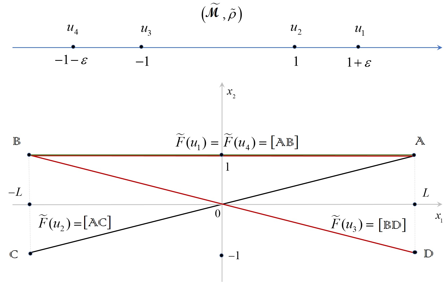
Fig. 1: The metric space $(\widetilde{{\mathcal{M}}},\tilde{\rho})$ and the set-valued mapping $\widetilde{F}$.

Let $\widetilde{{\mathcal{M}}}_{i}=\widetilde{{\mathcal{M}}}\setminus\{u_{i}\}$, $i=1,2,3,4$. We prove that the restriction $\widetilde{F}|_{\widetilde{{\mathcal{M}}}_{i}}$ has a Lipschitz selection $f_{i}:\widetilde{{\mathcal{M}}}_{i}\to{\mathbb{R}}^{2}$ with $\|f_{i}\|_{\operatorname{Lip}(\widetilde{{\mathcal{M}}}_{i},\ell^{2}_{\infty})}\leq 1$.

For $i=1$ we define $f_{1}$ by

$$f_{1}(u_{2})={\mathbb{C}},~{}~{}~{}~{}f_{1}(u_{3})=f_{1}(u_{4})={\mathbb{B}}\,.$$

Clearly, $f_{1}$ is a selection of $\widetilde{F}|_{\widetilde{{\mathcal{M}}}_{1}}$. Furthermore,

$$\|f_{1}(u_{2})-f_{1}(u_{3})\|_{\infty}=\|{\mathbb{C}}-{\mathbb{B}}\|_{\infty}=2=|u_{2}-u_{3}|=\tilde{\rho}(u_{2},u_{3}),$$

and

$$\|f_{1}(u_{2})-f_{1}(u_{4})\|_{\infty}=\|{\mathbb{C}}-{\mathbb{B}}\|_{\infty}=2\leq 2+\varepsilon=|u_{2}-u_{4}|=\tilde{\rho}(u_{2},u_{4})\,.$$

Combining these inequalities with the equality $f_{1}(u_{3})=f_{1}(u_{4})={\mathbb{B}}$ we conclude that the seminorm $\|f_{1}\|_{\operatorname{Lip}(\widetilde{{\mathcal{M}}}_{1},\ell^{2}_{\infty})}$ is bounded by $1$.

We define the functions $f_{i}$, $i=2,3,4$, by

$$f_{2}(u_{1})=f_{2}(u_{3})=f_{2}(u_{4})={\mathbb{B}},~{}~{}~{}~{}f_{3}(u_{1})=f_{3}(u_{2})=f_{3}(u_{4})={\mathbb{A}},$$

and $f_{4}(u_{1})=f_{4}(u_{2})={\mathbb{A}},~{}~{}~{}f_{4}(u_{3})={\mathbb{D}}\,.$

As in the case $i=1$, one can easily see that $f_{i}$ is a selection of $\widetilde{F}|_{\widetilde{{\mathcal{M}}}_{i}}$ with $\|f_{i}\|_{\operatorname{Lip}(\widetilde{{\mathcal{M}}}_{i},\ell^{2}_{\infty})}\leq 1$ for every $i=2,3,4$.

Statement 8.1

For every Lipschitz selection $f:\widetilde{{\mathcal{M}}}\to{\mathbb{R}}^{2}$ of the set-valued mapping $\widetilde{F}$ the following inequality $\|f\|_{\operatorname{Lip}(\widetilde{{\mathcal{M}}},\ell^{2}_{\infty})}\geq\lambda$ holds.

Proof. Let $\gamma=\|f\|_{\operatorname{Lip}(\widetilde{{\mathcal{M}}},\ell^{2}_{\infty})}$. Since $f$ is a Lipschitz selection of $\widetilde{F}$, the point $f(u_{i})\in\widetilde{F}(u_{i})$ for every $i=1,2,3,4$. Furthermore,

$$\|f(u_{i})-f(u_{j})\|_{\infty}\leq\gamma\tilde{\rho}(u_{i},u_{j})=\gamma|u_{i}-u_{j}|~{}~{}~{}\text{for every}~{}~{}~{}i,j=1,2,3,4.$$ (8.5)

Let us prove that $\gamma\geq\lambda$. By (8.5),

$$\|f(u_{1})-f(u_{2})\|_{\infty}\leq\gamma\,|u_{1}-u_{2}|=\gamma\varepsilon\,.$$ (8.6)

We also know that

$$f(u_{1})\in\widetilde{F}(u_{1})=[{\mathbb{A}}{\mathbb{B}}]~{}~{}~{}\text{and}~{}~{}~{}f(u_{2})\in\widetilde{F}(u_{2})=[{\mathbb{A}}{\mathbb{C}}]\,.$$ (8.7)

Let $f(u_{1})=(a_{1},a_{2})$ and $f(u_{2})=(b_{1},b_{2})$. Then, by (8.7), $|a_{1}|,\,|b_{1}|\leq L$, $a_{2}=1,|b_{2}|\leq 1$, and $b_{2}=b_{1}/L$ (because $(b_{1},b_{2})\in[{\mathbb{A}}{\mathbb{C}}]$).

By (8.6),

$$\max\{|a_{1}-b_{1}|,|a_{2}-b_{2}|\}=\|f(u_{1})-f(u_{2})\|_{\infty}\leq\gamma\varepsilon\,.$$

Hence,

$$0\leq 1-b_{2}=|a_{2}-b_{2}|\leq\gamma\varepsilon$$

so that $0\leq 1-b_{1}/L\leq\gamma\varepsilon$ proving that $0\leq L-b_{1}\leq\gamma\varepsilon\,L=\gamma\,.$ See (8.1). By this inequality,

$$\|{\mathbb{A}}-f(u_{2})\|_{\infty}=\max\{|L-b_{1}|,|1-b_{2}|\}\leq\gamma\,.$$

In the same way we prove that $\|{\mathbb{B}}-f(u_{3})\|_{\infty}\leq\gamma\,.$ Hence,

$$2L = \|{\mathbb{A}}-{\mathbb{B}}\|_{\infty}\leq\|{\mathbb{A}}-f(u_{2})\|_{\infty}+\|f(u_{2})-f(u_{3})\|_{\infty}+\|f(u_{3})-{\mathbb{B}}\|_{\infty}$$

$$\leq \gamma+\gamma\,|u_{2}-u_{3}|+\gamma=4\gamma\,.$$

But $L=2\lambda$ (see (8.1)), and the required inequality $\lambda\leq\gamma$ follows.

The proof of the statement is complete.         $\Box$

•  The sharp finiteness constant for $m=2$.

Let us prove that for the space $Y=\ell^{3}_{\infty}=({\mathbb{R}}^{3},\|\cdot\|_{\infty})$ the finiteness constant $N(2,Y)=8$ is sharp. Here $\|x\|_{\infty}=\max\{|x_{1}|,|x_{2}|,|x_{3}|\}$ for $x=(x_{1},x_{2},x_{3})\in{\mathbb{R}}^{3}$.

We will show that, given $\lambda\geq 1$ there exists a pseudometric space $({\mathcal{M}},\rho)$ and a set-valued mapping $F:{\mathcal{M}}\to{\mathcal{K}}_{2}({\mathbb{R}}^{3})$ such that the following is true: the restriction $F|_{{\mathcal{M}}^{\prime}}$ of $F$ to every subset ${\mathcal{M}}^{\prime}$ of ${\mathcal{M}}$ with $\#{\mathcal{M}}^{\prime}=7$ has a Lipschitz selection $f_{{\mathcal{M}}^{\prime}}:{\mathcal{M}}^{\prime}\to{\mathbb{R}}^{3}$ with $\|f_{{\mathcal{M}}^{\prime}}\|_{\operatorname{Lip}({\mathcal{M}}^{\prime},Y)}\leq 1$, but nevertheless $\|f\|_{\operatorname{Lip}({\mathcal{M}},Y)}\geq\lambda$ for every selection $f$ of $F$.

We again put $L=2\lambda$, $\varepsilon=1/L$, and $u_{1}=1+\varepsilon,~{}~{}u_{2}=1,~{}~{}u_{3}=-1,~{}~{}u_{4}=-1-\varepsilon\,.$

Let

$${\mathcal{M}}=\{u_{ik}:i=1,2,3,4,~{}~{}k=0,1\}$$

be an $8$-point set, and let $\psi:{\mathcal{M}}\to{\mathbb{R}}$ be a mapping defined by

$$\psi(u_{ik})=u_{i},~{}~{}~{}i=1,2,3,4,~{}~{}k=0,1.$$ (8.8)

We equip ${\mathcal{M}}$ with a pseudometric $\rho$ defined by

$$\rho(u,v)=|\psi(u)-\psi(v)|~{}~{}~{}\text{for all}~{}~{}~{}u,v\in{\mathcal{M}}\,.$$ (8.9)

Let

$$A=(L,1,0),~{}~{}~{}~{}A^{-}=(L,1,-\varepsilon),~{}~{}~{}B=(-L,1,0),~{}~{}~{}B^{-}=(-L,1,-\varepsilon),$$

and let

$$C=(-L,-1,0),~{}~{}~{}~{}C^{+}=(-L,-1,\varepsilon),~{}~{}~{}D=(L,-1,0),~{}~{}~{}D^{+}=(L,-1,\varepsilon)\,.$$

Given points $H_{i}\in{\mathbb{R}}^{3}$, $i=1,2,3,4$, we let $\operatorname{conv}(H_{1},...,H_{4})$ denote the convex hull of the set $\{H_{1},...,H_{4}\}$. We define the set-valued mapping $F:{\mathcal{M}}\to{\mathcal{K}}_{2}({\mathbb{R}}^{3})$ by letting

$$F(u_{i0})=\operatorname{conv}(A,B,C,D)~{}~{}~{}\text{for every}~{}~{}~{}~{}i=1,2,3,4.$$

Finally, we put

$$F(u_{11})=\operatorname{conv}(A,B,C^{+},D^{+}),~{}~{}~{}F(u_{21})=\operatorname{conv}(A,B^{-},C,D^{+})$$

and

$$F(u_{31})=\operatorname{conv}(A^{-},B,C^{+},D),~{}~{}~{}F(u_{41})=\operatorname{conv}(A,B,C^{+},D^{+})\,.$$

See Fig. 2 below.

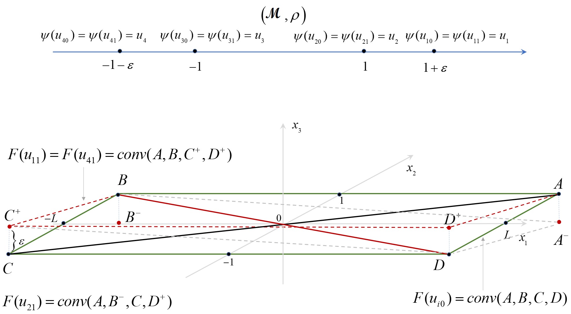
Fig. 2: The pseudometric space $({\mathcal{M}},\rho)$ and the set-valued mapping $F$.

Note that for each $u\in{\mathcal{M}}$ the set $F(u)\in{\mathcal{K}}_{2}({\mathbb{R}}^{3})$.

Let

$${\mathcal{M}}_{ik}={\mathcal{M}}\setminus\{u_{ik}\},~{}~{}~{}i=1,2,3,4,~{}~{}k=0,1\,.$$

We define a mapping $f_{ik}:{\mathcal{M}}_{ik}\to{\mathbb{R}}^{3}$ by letting

$$f_{10}(u)=\left\{\begin{array}[]{ll}C^{+},&\text{for}~{}~{}u=u_{11},\\ C\,,&\text{for}~{}~{}u=u_{20},u_{21},\\ B\,,&\text{for}~{}~{}u=u_{30},u_{31},u_{40},u_{41}\end{array}\right.~{}~{}~{}~{}\text{and}~{}~{}~{}~{}f_{11}(u)=\left\{\begin{array}[]{ll}B\,,&\text{for}~{}~{}u=u_{30},u_{31},u_{40},u_{41},\\ C\,,&\text{for}~{}~{}u=u_{10},u_{20},u_{21}.\end{array}\right.$$

We also put

$$f_{20}(u)=\left\{\begin{array}[]{ll}B^{-},&\text{for}~{}~{}u=u_{21},\\ B\,,&\text{for}~{}~{}u\in{\mathcal{M}}\setminus\{u_{20},u_{21}\},\end{array}\right.~{}~{}~{}~{}~{}~{}~{}~{}f_{21}\equiv B,$$

and

$$f_{30}(u)=\left\{\begin{array}[]{ll}A^{-},&\text{for}~{}~{}u=u_{31},\\ A\,,&\text{for}~{}~{}u\in{\mathcal{M}}\setminus\{u_{30},u_{31}\},\end{array}\right.~{}~{}~{}~{}~{}~{}~{}~{}f_{31}\equiv A\,.$$

Finally, we define functions $f_{40}$ and $f_{41}$ by

$$f_{40}(u)=\left\{\begin{array}[]{ll}A,&\text{for}~{}~{}u=u_{10},u_{11},u_{20},u_{21},\\ D\,,&\text{for}~{}~{}u=u_{30},u_{31},\\ D^{+}\,,&\text{for}~{}~{}u=u_{41},\end{array}\right.~{}~{}~{}~{}\text{and}~{}~{}~{}~{}f_{41}(u)=\left\{\begin{array}[]{ll}A\,,&\text{for}~{}~{}u=u_{10},u_{11},u_{20},u_{21},\\ D\,,&\text{for}~{}~{}u=u_{30},u_{31},u_{40}.\end{array}\right.$$

The reader can easily check that each function $f_{ik}:{\mathcal{M}}_{ik}\to{\mathbb{R}}^{3}$ is a selection of the restriction $F|_{{\mathcal{M}}_{ik}}$ with $\|f_{ik}\|_{\operatorname{Lip}({\mathcal{M}}_{ik},\ell^{3}_{\infty})}\leq 1$.

Let us prove an analog of Statement 8.1 for the pseudometric space $({\mathcal{M}},\rho)$ and the set-valued mapping $F:{\mathcal{M}}\to{\mathcal{K}}_{2}({\mathbb{R}}^{3})$.

Statement 8.2

For every Lipschitz selection $f:{\mathcal{M}}\to{\mathbb{R}}^{3}$ of $F$ the following inequality

$$\|f\|_{\operatorname{Lip}({\mathcal{M}},\ell^{3}_{\infty})}\geq\lambda$$

holds.

Proof. Let $f:{\mathcal{M}}\to{\mathbb{R}}^{3}$ be a selection of $F$ with $\|f\|_{\operatorname{Lip}({\mathcal{M}},\ell^{3}_{\infty})}=\gamma$. Thus $f(u_{ik})\in F(u_{ik})$ for every $i=1,2,3,4$,  $k=0,1$, and $f$ satisfies the Lipschitz condition with the constant $\gamma$. In particular,

$$\|f(u_{10})-f(u_{11})\|_{\infty}\leq\gamma\,\rho(u_{10},u_{11})=0$$

(see (8.8) and (8.9)), so that $f(u_{10})=f(u_{11})$.

Let $a_{1}=f(u_{10})=f(u_{11})$. Then

$$a_{1}=f(u_{10})\in F(u_{10})=\operatorname{conv}(A,B,C,D)~{}~{}~{}\text{and}~{}~{}~{}a_{1}=f(u_{11})\in F(u_{11})=\operatorname{conv}(A,B,C^{+},D^{+})$$

so that

$$a_{1}\in\operatorname{conv}(A,B,C,D)\,{\bigcap}\operatorname{conv}(A,B,C^{+},D^{+})=[AB].$$ (8.10)

In a similar way we prove that $f(u_{i0})=f(u_{i1})$ for every $i=2,3,4$, and the points

$$a_{i}=f(u_{i0})=f(u_{i1}),~{}~{}~{}i=2,3,4,$$

have the following property:

$$a_{2}\in[AC],~{}~{}~{}~{}a_{3}\in[BD],~{}~{}~{}~{}a_{4}\in[AB]\,.$$ (8.11)

Let $(\widetilde{{\mathcal{M}}},\tilde{\rho})$ be the metric space defined by formulae (8.2) and (8.3), and let $\tilde{f}:\widetilde{{\mathcal{M}}}\to{\mathbb{R}}^{2}$ be a mapping defined by

$$\tilde{f}(u_{i})=a_{i},~{}~{}~{}~{}~{}i=1,2,3,4.$$

Thus

$$\tilde{f}(u_{i})=f(u_{i0})=f(u_{i1})~{}~{}~{}\text{for each}~{}~{}~{}i=1,2,3,4.$$

This formula together with definition (8.2) of the metric space $\widetilde{{\mathcal{M}}}$ and definitions (8.8), (8.9) of the pseudometric space ${\mathcal{M}}$ implies the following equality:

$$\gamma=\|f\|_{\operatorname{Lip}({\mathcal{M}},\ell^{3}_{\infty})}=\|\tilde{f}\|_{\operatorname{Lip}(\widetilde{{\mathcal{M}}},\ell^{2}_{\infty})}.$$ (8.12)

Furthermore, by (8.10) and (8.11), $\tilde{f}$ is a selection of the set-valued mapping $\widetilde{F}:\widetilde{{\mathcal{M}}}\to{\mathcal{K}}_{1}({\mathbb{R}}^{2})$ defined by (8.4). Therefore, by Statement 8.1, $\|\tilde{f}\|_{\operatorname{Lip}(\widetilde{{\mathcal{M}}},\ell^{2}_{\infty})}\geq\lambda.$

This inequality together with (8.12) implies the required inequality $\|f\|_{\operatorname{Lip}({\mathcal{M}},\ell^{3}_{\infty})}\geq\lambda$ completing the proof of Statement 8.2.         $\Box$

8.2. Final remarks.

We finish Section 8 with three remarks. The first concerns connections between Steiner-type points, see Theorem 1.6 and Section 7, and the finiteness principle for Lipschitz selections given in Theorem 1.1. The second remark deals with a slight generalization of Theorem 1.1 for the case of set-valued mappings with closed images. The third one shows that in general the finiteness principle does not hold for quasimetric spaces.

•  Steiner-type points and the finiteness principle for Lipschitz selections.

Let $Y$ be a Banach space. Given $m\in{\mathbb{N}}$ let ${\mathcal{M}}={\mathcal{K}}_{m}(Y)$ be the family of all non-empty convex compact subsets of $Y$ of affine dimension at most $m$ equipped with the Hausdorff distance $\rho=\operatorname{d_{H}}$.

Let $F:{\mathcal{M}}\to{\mathcal{K}}_{m}(Y)$ be the “identity” mapping on ${\mathcal{K}}_{m}(Y)$, i.e.,

$$F(K)=K~{}~{}~{}~{}\text{for every}~{}~{}K\in{\mathcal{K}}_{m}(Y).$$

By Theorem 1.6, this mapping has a selection $S_{Y}:{\mathcal{M}}\to Y$ whose $\operatorname{d_{H}}$-Lipschitz seminorm is bounded by a constant $\gamma=\gamma(m)$ depending only on $m$.

Let us see that this statement is a particular case of the Finiteness Principle for Lipschitz Selections proven in Theorem 1.1. In other words, let us prove that the mapping $F$ satisfies the hypothesis of Theorem 1.1 (with respect to a metric $\theta\operatorname{d_{H}}$ with a certain $\theta=\theta(m)$).

Claim 8.3

For every subset ${\mathcal{M}}^{\prime}\subset{\mathcal{M}}$ with $\#{\mathcal{M}}^{\prime}\leq N(m,Y)$ the restriction $F|_{{\mathcal{M}}^{\prime}}$ has a $\operatorname{d_{H}}$-Lipschitz selection $f_{{\mathcal{M}}^{\prime}}:{\mathcal{M}}^{\prime}\to Y$ with $\|f_{{\mathcal{M}}^{\prime}}\|_{\operatorname{Lip}(({\mathcal{M}}^{\prime},\operatorname{d_{H}}),Y)}\leq\theta$ where $\theta=\theta(m)$ is a constant depending only on $m$.

Proof. By Proposition 6.6, there exists a tree $T=({\mathcal{M}}^{\prime},E)$ such that

$$\operatorname{d_{H}}(K,K^{\prime})\leq d_{T}(K,K^{\prime})\leq\theta\,\operatorname{d_{H}}(K,K^{\prime})~{}~{}~{}\text{for every}~{}~{}~{}K,K^{\prime}\in{\mathcal{M}}^{\prime}.$$ (8.13)

Here $\theta=\theta(\#{\mathcal{M}}^{\prime})$. Since $\#{\mathcal{M}}^{\prime}\leq N(m,Y)\leq 2^{m+1}$, the constant $\theta$ depends only on $m$.

Recall that $d_{T}$ is a tree metric defined by (6.15) and (6.16). Thus

$$d_{T}(K,K^{\prime})=\operatorname{d_{H}}(K,K^{\prime})$$

for every $K,K^{\prime}\in{\mathcal{M}}^{\prime}$ joined by an edge in $T$ ($K\leftrightarrow K^{\prime}$).

Let us show that there exists a $d_{T}$-Lipschitz selection $f:{\mathcal{M}}^{\prime}\to Y$ of $F$ with the $d_{T}$-Lipschitz seminorm $\|f\|_{\operatorname{Lip}(({\mathcal{M}}^{\prime},d_{T}),Y)}\leq 1$.

Fix a set $K_{0}\in{\mathcal{M}}^{\prime}$ and a point $x_{0}\in K_{0}$, and put $f(K_{0})=x_{0}$. Let $J^{(0)}=K_{0}$ and let

$$J_{0}(T)=\{K\in{\mathcal{M}}^{\prime}:K\leftrightarrow K_{0}~{}~{}~{}\text{in}~{}~{}~{}T\}$$

be the family of all neighbors of $K_{0}$ in $T$. Let

$$J^{(1)}=J^{(0)}\cup J_{0}(T).$$

Given $K,K^{\prime}\in{\mathcal{M}}={\mathcal{K}}_{m}(Y)$ we let $A(K,K^{\prime})$ denote a point nearest to $K^{\prime}$ on $K$. Then we define a mapping $f_{1}:J^{(1)}\to Y$ by letting $f_{1}(K_{0})=x_{0}$ and $f_{1}(K)=A(K,K_{0})$ provided $K\in J_{0}(T)$.

Then, by definition of the Hausdorff distance (see (5.2)),

$$\|f_{1}(K_{0})-f_{1}(K)\|\leq\operatorname{d_{H}}(K_{0},K)=d_{T}(K_{0},K),~{}~{}~{}K\in J_{0}(T).$$

Thus,

$$\|f_{1}(K)-f_{1}(K^{\prime})\|\leq d_{T}(K,K^{\prime})~{}~{}~{}\text{for all}~{}~{}~{}K,K^{\prime}\in J^{(1)},~{}K\leftrightarrow K^{\prime}~{}~{}~{}\text{in}~{}~{}~{}T.$$ (8.14)

Using the same idea, at the next step of this construction we extend $f_{1}$ from $J^{(1)}$ to a set

$$J^{(2)}=J^{(1)}\cup J_{1}(T)$$

where

$$J_{1}(T)=\{K\in{\mathcal{M}}^{\prime}\setminus J^{(1)}:\exists\,\,K^{\prime}\in J^{(1)}~{}~{}~{}\text{such that}~{}~{}~{}K^{\prime}\leftrightarrow K~{}~{}~{}\text{in}~{}~{}~{}T\}.$$ (8.15)

We define a mapping $f_{2}:J^{(2)}\to Y$ by letting

$$f_{2}|_{J^{(1)}}=f_{1}~{}~{}~{}\text{and}~{}~{}~{}f_{2}(K)=A(K,K^{\prime})$$

provided $K\in{\mathcal{M}}^{\prime}\setminus J^{(1)}$ and $K^{\prime}\in J^{(1)}$, $K^{\prime}\leftrightarrow K$ in $T$. Clearly, by (8.15), such a set $K^{\prime}\in J^{(1)}$ exists. Since $T$ is a tree, $K^{\prime}$ is unique, so that the mapping $f_{2}$ is well defined.

Furthermore, one can easily see that $f_{2}$ has a property similar to (8.14), i.e.,

$$\|f_{2}(K)-f_{2}(K^{\prime})\|\leq d_{T}(K,K^{\prime})~{}~{}~{}\text{for all}~{}~{}~{}K,K^{\prime}\in J^{(2)},~{}K\leftrightarrow K^{\prime}~{}~{}~{}\text{in}~{}~{}~{}T.$$

We continue this extension procedure. At a certain step of this process, say at a step $k$ with $1\leq k\leq\#{\mathcal{M}}$, the set $J^{(k)}$ will coincide with ${\mathcal{M}}^{\prime}$ so that the mapping $f=f_{k}$ will be well defined on all of the set ${\mathcal{M}}^{\prime}$. This mapping provides a selection of the restriction $F|_{{\mathcal{M}}^{\prime}}$, i.e., $f(K)\in K$ for each $K\in{\mathcal{M}}^{\prime}$. Furthermore, it satisfies inequality

$$\|f(K)-f(K^{\prime})\|\leq d_{T}(K,K^{\prime})$$

for all $K,K^{\prime}\in{\mathcal{M}}^{\prime}$ joined by an edge in $T$. This proves that $f$ is the required $d_{T}$-Lipschitz selection of $F$ on ${\mathcal{M}}^{\prime}$ with the $d_{T}$-Lipschitz seminorm bounded by $1$.

Hence, by (8.13), the $\operatorname{d_{H}}$-Lipschitz seminorm of $f$ on ${\mathcal{M}}^{\prime}$ is bounded by $\theta$, and the proof of the claim is complete.         $\Box$

Claim 8.3 shows that Theorem 1.6 can be considered as a particular case of our main result, Theorem 1.1, which is applied to the metric space $({\mathcal{K}}_{m}(Y),\operatorname{d_{H}})$. In general, this metric space has the same complexity as an $L_{\infty}$-space. In particular, $({\mathcal{K}}_{m}(Y),\operatorname{d_{H}})$ may be non-doubling (even for two dimensional $Y$) and may have infinite Nagata dimension. In these cases we are unable to prove Theorem 1.6 using the ideas and methods developed in Sections 2-4.

Thus, analyzing the scheme of the proof of Theorem 1.1, we observe that this proof is actually based on solutions of the Lipschitz selection problem for two independent particular cases of this problem, namely, for metric trees, see Theorem 1.4 and Sections 2-4, and for the metric space $({\mathcal{K}}_{m}(Y),\operatorname{d_{H}})$, see Section 7. Theorem 1.5 proven in Section 5 provides a certain “bridge” between these two independent results (i.e., Theorems 1.4 and 1.6). Combining all these results, we finally obtain a proof of Theorem 1.1 in the general case.

•  Generalization of the finiteness principle: set-valued mappings with closed images.

In Theorem 1.1 we prove the finiteness principle for set-valued mappings $F$ whose values are convex compact sets with affine dimension bounded by $m$. The following claim states that this family of sets can be slightly extended.

Statement 8.4

Theorem 1.1 holds provided the requirement $F:{\mathcal{M}}\to{\mathcal{K}}_{m}(Y)$ in its formulation is replaced with the following one: for every $x\in{\mathcal{M}}$ the set $F(x)$ is a closed convex subset of $Y$ of dimension at most $m$, and there exists $x_{0}\in{\mathcal{M}}$ such that $F(x_{0})$ is bounded.

Proof. Let $({\mathcal{M}},\rho)$ be a pseudometric space and let $F$ be a set-valued mapping on ${\mathcal{M}}$ satisfying the hypothesis of the present statement such that for every subset ${\mathcal{M}}^{\prime}\subset{\mathcal{M}}$ consisting of at most $N(m,Y)$ points, the restriction $F|_{{\mathcal{M}}^{\prime}}$ of $F$ to ${\mathcal{M}}^{\prime}$ has a Lipschitz selection $f_{{\mathcal{M}}^{\prime}}:{\mathcal{M}}^{\prime}\to Y$ with $\|f_{{\mathcal{M}}^{\prime}}\|_{\operatorname{Lip}({\mathcal{M}}^{\prime},Y)}\leq 1$. We have to prove the existence of a Lipschitz selection of $F$ on ${\mathcal{M}}$ whose Lipschitz seminorm is bounded by a constant depending only on $m$.

By Theorem 1.7, there exists a constant $\alpha=\alpha(m)\geq 1$ depending only on $m$, such that for every subset $\widetilde{{\mathcal{M}}}\subset{\mathcal{M}}$ with $\#\widetilde{{\mathcal{M}}}\leq N(m,Y)+1$, the restriction $F|_{\widetilde{{\mathcal{M}}}}$ has a Lipschitz selection $f_{\widetilde{{\mathcal{M}}}}:\widetilde{{\mathcal{M}}}\to Y$ with $\|f_{\widetilde{{\mathcal{M}}}}\|_{\operatorname{Lip}(\widetilde{{\mathcal{M}}},Y)}\leq\alpha$.

We introduce a new set-valued mapping $\widetilde{F}$ on ${\mathcal{M}}$ by letting

$$\widetilde{F}(x)=F(x)\cap[F(x_{0})+B_{Y}(0,\alpha\rho(x_{0},x))],~{}~{}~{}~{}x\in{\mathcal{M}}\,.$$ (8.16)

We prove that $\widetilde{F}(x)$ is a non-empty and belongs to ${\mathcal{K}}_{m}(Y)$ for every $x\in{\mathcal{M}}$. Clearly, it is true for $x=x_{0}$ (because $F(x_{0})$ is convex closed bounded and finite dimensional). Let $x\neq x_{0}$ and let ${\mathcal{M}}^{\prime}=\{x,x_{0}\}$. Since $\#{\mathcal{M}}^{\prime}=2\leq N(m,Y)$, there exists a function $f_{{\mathcal{M}}^{\prime}}:{\mathcal{M}}^{\prime}\to Y$ such that $f_{{\mathcal{M}}^{\prime}}(x)\in F(x)$, $f_{{\mathcal{M}}^{\prime}}(x_{0})\in F(x_{0})$, and

$$\|f_{{\mathcal{M}}^{\prime}}(x)-f_{{\mathcal{M}}^{\prime}}(x_{0})\|\leq\rho(x,x_{0})\,.$$

Hence, by (8.16), $f_{{\mathcal{M}}^{\prime}}(x)\in\widetilde{F}(x)$ proving that $\widetilde{F}(x)\neq\emptyset$.

By formula (8.16), $\widetilde{F}(x)$ is a convex closed finite dimensional subset of $Y$ of affine dimension at most $m$. Since $F(x_{0})$ is bounded, $\widetilde{F}(x)$ is bounded as well, so that $\widetilde{F}(x)$ is compact.

Thus $\widetilde{F}:{\mathcal{M}}\to{\mathcal{K}}_{m}(Y)$. Let us show that for each ${\mathcal{M}}^{\prime}\subset{\mathcal{M}}$ with $\#{\mathcal{M}}^{\prime}\leq N(m,Y)$, the restriction $\widetilde{F}|_{{\mathcal{M}}^{\prime}}$ of $\widetilde{F}$ to ${\mathcal{M}}^{\prime}$ has a Lipschitz selection $\tilde{f}_{{\mathcal{M}}^{\prime}}:{\mathcal{M}}^{\prime}\to Y$ with $\|\tilde{f}_{{\mathcal{M}}^{\prime}}\|_{\operatorname{Lip}({\mathcal{M}}^{\prime},Y)}\leq\alpha$.

Indeed, let $\widetilde{{\mathcal{M}}}={\mathcal{M}}^{\prime}\cup\{x_{0}\}$. Then $\#\widetilde{{\mathcal{M}}}\leq N(m,Y)+1$ so that the restriction $F|_{\widetilde{{\mathcal{M}}}}$ has a Lipschitz selection $f_{\widetilde{{\mathcal{M}}}}:\widetilde{{\mathcal{M}}}\to Y$ with $\|f_{\widetilde{{\mathcal{M}}}}\|_{\operatorname{Lip}(\widetilde{{\mathcal{M}}},Y)}\leq\alpha$. Let

$$\tilde{f}_{{\mathcal{M}}^{\prime}}=f_{\widetilde{{\mathcal{M}}}}\,|_{\,{\mathcal{M}}^{\prime}}.$$

Then $\tilde{f}_{{\mathcal{M}}^{\prime}}(x)\in F(x)$ and

$$\|\tilde{f}_{{\mathcal{M}}^{\prime}}(x)-\tilde{f}_{{\mathcal{M}}^{\prime}}(x_{0})\|\leq\alpha\rho(x,x_{0})~{}~{}~{}~{}\text{for every}~{}~{}~{}x\in{\mathcal{M}}^{\prime}\,.$$

Hence, by (8.16), $\tilde{f}_{{\mathcal{M}}^{\prime}}(x)\in\widetilde{F}(x)$ on ${\mathcal{M}}^{\prime}$, so that $\tilde{f}_{{\mathcal{M}}^{\prime}}$ is a selection of $\widetilde{F}|_{{\mathcal{M}}^{\prime}}$. It is also clear that

$$\|\tilde{f}_{{\mathcal{M}}^{\prime}}\|_{\operatorname{Lip}({\mathcal{M}}^{\prime},Y)}\leq\|f_{\widetilde{{\mathcal{M}}}}\|_{\operatorname{Lip}(\widetilde{{\mathcal{M}}},Y)}\leq\alpha,$$

proving that $\tilde{f}_{{\mathcal{M}}^{\prime}}$ is the required Lipschitz selection of $\widetilde{F}|_{{\mathcal{M}}^{\prime}}$.

This enables us to apply Theorem 1.1 to the pseudometric space $({\mathcal{M}},\alpha\rho)$ and to the set-valued mapping $\widetilde{F}:{\mathcal{M}}\to{\mathcal{K}}_{m}(Y)$. By this theorem, there exists an $\alpha\rho$-Lipschitz selection $f:{\mathcal{M}}\to Y$ of $\widetilde{F}$ with $\alpha\rho$-Lipschitz seminorm at most $\gamma$. Here $\gamma=\gamma(m)$ is a constant depending only on $m$.

Clearly, $f$ is a $\rho$-Lipschitz selection of $\widetilde{F}$ whose $\rho$-Lipschitz seminorm is bounded by $\alpha\gamma$. Since $\widetilde{F}(x)\subset F(x)$ for every $x\in{\mathcal{M}}$ (see (8.16)), $f$ is also a $\rho$-Lipschitz selection of $F$ with the seminorm $\|f\|_{\operatorname{Lip}(({\mathcal{M}},\rho),Y)}\leq\alpha\gamma$.

The proof of Statement 8.4 is complete.         $\Box$

Statement 8.4 implies the following result.

Theorem 8.5

Theorem 1.1 holds provided the requirement $F:{\mathcal{M}}\to{\mathcal{K}}_{m}(Y)$ in its formulation is replaced with $F:{\mathcal{M}}\to{\mathcal{K}}_{m}(Y)\cup\operatorname{{\it Aff}}_{m}(Y)$.

We recall that $\operatorname{{\it Aff}}_{m}(Y)$ denotes the family of all affine subspaces of $Y$ of dimension at most $m$.

Proof. The result follows from [40] whenever $F:{\mathcal{M}}\to\operatorname{{\it Aff}}_{m}(Y)$, and from Statement 8.4 whenever there exists $x_{0}\in{\mathcal{M}}$ such that $F(x_{0})\in{\mathcal{K}}_{m}(Y)$.         $\Box$

•  Quasimetric spaces.

Recall that a quasimetric on a set ${\mathcal{M}}$ is a function $\rho:{\mathcal{M}}\times{\mathcal{M}}\to[0,\infty)$ that is symmetric, vanishes if and only if $x=y$, and satisfies, for some $K\geq 1$, the quasi-triangle inequality

$$\rho(x,y)\leq K(\,\rho(x,z)+\rho(z,y))~{}~{}~{}~{}\text{for all}~{}~{}~{}x,y,z\in{\mathcal{M}}\,.$$

We refer to the pair $({\mathcal{M}},\rho)$ as a quasimetric space.

In Theorem 1.1 we prove the finiteness principle for set-valued mappings defined on metric spaces. The following natural question arises: does the finiteness principle hold for set-valued mappings defined on quasimetric spaces?

The example below shows that in general the answer to this question is negative.

Example 8.6

Let $Y={\mathbb{R}}$. Let ${\mathcal{M}}=[0,1]$ and let $\rho(x,y)=|x-y|^{2}$, $x,y\in{\mathcal{M}}$. Clearly, $\rho$ is a quasimetric on ${\mathcal{M}}$ satisfying the quasi-triangle inequality

$$\rho(x,y)\leq 2(\,\rho(x,z)+\rho(z,y)),~{}~{}~{}~{}x,y,z\in{\mathcal{M}}\,.$$

Let $N>1$ be a positive integer, and let $F:{\mathcal{M}}\to{\mathcal{K}}_{1}({\mathbb{R}})$ be a set valued mapping defined by

$$F(x)=\left\{\begin{array}[]{ll}\{0\},&\text{if}~{}~{}x=0,\\ {[0,1]},&\text{if}~{}~{}x\in(0,1),\\ \{N^{-2}\},&\text{if}~{}~{}x=1.\end{array}\right.$$ (8.20)

Claim 8.7

For every subset ${\mathcal{M}}^{\prime}\subset{\mathcal{M}}$ consisting of at most $N$ points, the restriction $F|_{{\mathcal{M}}^{\prime}}$ of $F$ to ${\mathcal{M}}^{\prime}$ has a $\rho$-Lipschitz selection $f_{{\mathcal{M}}^{\prime}}:{\mathcal{M}}^{\prime}\to{\mathbb{R}}$ with $\|f_{{\mathcal{M}}^{\prime}}\|_{\operatorname{Lip}({\mathcal{M}}^{\prime},{\mathbb{R}})}\leq 1$. Nevertheless, a $\rho$-Lipschitz selection of $F$ on ${\mathcal{M}}$ does not exist.

Proof. Let ${\mathcal{M}}^{\prime}=\{x_{i}:i=1,...,N\}$ where $0\leq x_{1}<...<x_{N}\leq 1$. If $x_{1}>0$ or $x_{N}<1$, we put $f_{{\mathcal{M}}^{\prime}}\equiv 0$ or $f_{{\mathcal{M}}^{\prime}}\equiv N^{-2}$ respectively. Clearly, by (8.20), in these cases $f_{{\mathcal{M}}^{\prime}}$ is a selection of $F|_{{\mathcal{M}}^{\prime}}$ with $\|f_{{\mathcal{M}}^{\prime}}\|_{\operatorname{Lip}({\mathcal{M}}^{\prime},{\mathbb{R}})}=0$.

Now let $x_{1}=0$ and $x_{N}=1$. Then there exists $i_{0}\in\{1,...,N-1\}$ such that $x_{i_{0}+1}-x_{i_{0}}\geq 1/N$. In fact, otherwise $x_{i+1}-x_{i}<1/N$ for every $i=1,...,N-1$, so that $1=x_{N}-x_{1}<(N-1)/N<1$, a contradiction.

Let

$$f_{{\mathcal{M}}^{\prime}}(x_{i})=\left\{\begin{array}[]{ll}0,&\text{if}~{}~{}1\leq i\leq i_{0},\vspace*{1mm}\\ N^{-2},&\text{if}~{}~{}i_{0}<i\leq N.\end{array}\right.$$ (8.23)

Then $f_{{\mathcal{M}}^{\prime}}(0)=f_{{\mathcal{M}}^{\prime}}(x_{1})=0\in F(0)$, $f_{{\mathcal{M}}^{\prime}}(1)=f_{{\mathcal{M}}^{\prime}}(x_{N})=N^{-2}\in F(1)$, and $f_{{\mathcal{M}}^{\prime}}(x_{i})\in[0,1]=F(x_{i})$ if $1<i<N$, proving that $f_{{\mathcal{M}}^{\prime}}$ is a selection of $F|_{{\mathcal{M}}^{\prime}}$.

Let us estimate its $\rho$-Lipschitz seminorm. Let $x=x_{i},y=x_{j}\in{\mathcal{M}}^{\prime}$, $x<y$. If $1\leq i,j\leq i_{0}$ or $i_{0}<i,j\leq N$, then, by (8.23), $f_{{\mathcal{M}}^{\prime}}(x)=f_{{\mathcal{M}}^{\prime}}(y)$. Let $1\leq i\leq i_{0}$ and $i_{0}<j\leq N$, so that $|x-y|\geq x_{i_{0}+1}-x_{i_{0}}\geq 1/N$. Then, by (8.23),

$$|f_{{\mathcal{M}}^{\prime}}(x)-f_{{\mathcal{M}}^{\prime}}(y)|=1/N^{2}\leq|x-y|^{2}=\rho(x,y)$$

proving that $\|f_{{\mathcal{M}}^{\prime}}\|_{\operatorname{Lip}({\mathcal{M}}^{\prime},{\mathbb{R}})}\leq 1$. Thus, $f_{{\mathcal{M}}^{\prime}}$ is the required $\rho$-Lipschitz selection of $F|_{{\mathcal{M}}^{\prime}}$.

We prove that a $\rho$-Lipschitz selection of $F$ on all of ${\mathcal{M}}$ does not exists. Indeed, if $f:{\mathcal{M}}\to{\mathbb{R}}$ is such a selection with $\|f\|_{\operatorname{Lip}({\mathcal{M}},{\mathbb{R}})}=\gamma$ then

$$|f(x)-f(y)|\leq\gamma\rho(x,y)=\gamma|x-y|^{2}~{}~{}~{}~{}\text{for all}~{}~{}~{}~{}x,y\in[0,1]$$

so that $f$ is a constant function on $[0,1]$. In particular, $f(0)=f(1)$.

On the other hand, $f$ is a selection of $F$ on ${\mathcal{M}}$ so that $f(0)\in F(0)=\{0\}$ and

$$f(1)\in F(1)=\{1/N^{2}\}.$$

Hence, $f(0)=0$ and $f(1)=1/N^{2}$ so that $f(0)\neq f(1)$, a contradiction.

The proof of the claim is complete.         $\Box$

References

[1] P. Assouad, Sur la distance de Nagata, C. R. Acad. Sci. Paris Sér. I Math. 294 (1982), no. 1, 31–34.
[2] J.-P. Aubin, A. Cellina,
Differential inclusions, Springer, Berlin, 1984.
[3] Y. Benyamini, J. Lindenstrauss, Geometric nonlinear functional analysis, Vol. 1, in: AMS Colloquium Publications, 48. AMS, Providence, RI, 2000. xii+488 pp.
[4] N. Brodskiy, J. Dydak, J. Higes, A. Mitra, Assouad-Nagata dimension via Lipschitz extensions, Israel J. Math. 171 (2009), 405–423.
[5] A. Brudnyi and Yu. Brudnyi, Methods of Geometric Analysis in extension and trace problems,
Vol. I, Monographs in Mathematics, Vol. 102, Springer, Basel, 2012.
[6] Y. Brudnyi, P. Shvartsman, Generalizations of Whitney’s extension theorem. Internat. Math. Res. Notices (1994), no. 3, 129–139.
[7] Yu. Brudnyi and P. Shvartsman, The trace of jet space to an arbitrary closed subset of , Trans. Amer. Math. Soc. 350 (1998), no. 4, 1519–1553.
[8] Yu. Brudnyi and P. Shvartsman,
Whitney Extension Problem for Multivariate
-functions, Trans. Amer. Math. Soc. 353 No. 6, (2001) 2487–2512.
[9] P. B. Callahan, S. R. Kosaraju, A decomposition of multidimensional point sets with
applications to -nearest-neighbors and -body potential fields, J. Assoc. for Computing Machinery 42 (1995) 67–90.
[10] L. Danzer, B. Grünbaum, V. Klee, Helly’s Theorem and its relatives, in: AMS Symposium on Convexity, Seattle, Proceedings of Symposium on Pure Mathematics, Vol. 7, Amer. Math. Soc., Providence, RI, 1963, pp. 101–180.
[11] C. Fefferman, A sharp form of Whitney extension theorem, Annals of Math. 161, No. 1 (2005) 509–577.
[12] C. Fefferman, A Generalized Sharp Whitney Theorem for Jets, Rev. Mat. Iberoamericana 21, no.2, (2005) 577–688.
[13] C. Fefferman, Whitney extension problem for , Annals of Math. 164, no. 1, (2006) 313–359.
[14] C. Fefferman and B. Klartag, Fitting a -smooth function to data I, Annals of Math. 169, No. 1, (2009) 315–346.
[15] C. Fefferman and B. Klartag, Fitting a -smooth function to data II, Revista Mat. Iberoamericana 25, No. 1, (2009) 49–273.
[16] C. Fefferman, Fitting a -smooth function to data III, Annals of Math. 170, No.1, (2009) 427–441.
[17] C. Fefferman, Whitney extension problems and interpolation of data, Bulletin A.M.S. 46, no. 2 (2009) 207–220.
[18] C. Fefferman, A. Israel, G. K. Luli, Finiteness principles for smooth selection, Geom. Funct. Anal. 26 (2016), no. 2, 422–477.
[19] C. Fefferman, A. Israel, G. K. Luli, Finiteness principles for and Lipschitz selection, 82 pp., Whitney Extension Problems: and Sobolev functions on subsets of , The 9th Whitney Problems Workshop, May–June 2016, Haifa, Israel.
http://www.math.technion.ac.il/Site/events/EvntOffices/event.php?eid=eo108
[20] C. Fefferman, A. Israel, G. K. Luli,
Interpolation of data by smooth non-negative functions, Rev. Mat. Iberoam. 33 (2017), no. 1, 305–324.
[21] A. Gaifullin, Center of union of identical convex centrally symmetric sets. Preprint.
[22] S. Har-Peled, M. Mendel, Fast Construction of Nets in Low-Dimensional Metrics and Their Applications, SIAM J. Comput. 35 (2006), no. 5, 1148–1184.
[23] U. Lang, T. Schlichenmaier, Nagata dimension, quasisymmetric embeddings, and Lipschitz extensions, Int. Math. Res. Not. (2005), no. 58, 3625–3655.
[24] E. Le Donne, T. Rajala, Assouad dimension, Nagata dimension, and uniformly close metric tangents, Indiana Univ. Math. J. 64 (2015) 21–54.
[25] H. Minkowski, Allgemeine Lehrsätze über die konvexen Polyeder, in: Nachr. Ges. Wiss. Göttingen, 198–219. Gessamelte Abhandlungen, vol. II, Teubner, Leipzig, 1911, 103–121.
[26] J. Nagata, Note on dimension theory for metric spaces, Fund. Math. 45 (1958) 143–181.
[27] E. D. Posicelskii, Lipschitzian mappings in the space of convex bodies, Optimizacija 4 (21) (1971)
83–89 (in Russian).
[28] K. Przesławski, Centres of Convex Sets in Metrics, J. Approx. Theory 85 (1996) 288–296.
[29] K. Przesławski, L. E. Rybinski, Concepts of lower semicontinuity and continuous selections for convex valued multifunctions, J. Approx. Theory 68 (1992) 262–282.
[30] K. Przesławski, D. Yost, Continuity properties of selectors and Michael’s theorem, Mich. Math. J. 36 (1989) 113–134.
[31] R. Schneider, On Steiner points of convex bodies, Israel J. Math. 9 (1971) 241–249.
[32] R. Schneider, Convex bodies: the Brunn-Minkowski theory, in: Encyclopedia of Mathematics and its Applications, 44. Cambridge Univ. Press, Cambridge, 1993.
[33] G. C. Shephard, The Steiner point of a convex polytope, Canad. J. Math. 18 (1966) 1294–1300.
[34] G. C. Shephard, R. J. Webster, Metrics for sets of convex bodies, Mathematika 12 (1965) 73–88.
[35] P. Shvartsman, Lipschitz sections of multivalued mappings. (Russian) Studies in the theory of functions of several real variables (Russian), 121–132, 149, Yaroslav. Gos. Univ., Yaroslavl’, 1986.
[36] P. Shvartsman, On the traces of functions of the Zygmund class, Sib. Mat. Zh. 28, No. 5, (1987) 203–215; English transl. in Sib. Math. J. 28 (1987) 853–863.
[37] P. Shvartsman, -functionals of weighted Lipschitz spaces and Lipschitz selections of multivalued mappings. Interpolation spaces and related topics (Haifa, 1990), 245–268, Israel Math. Conf. Proc., 5, Bar-Ilan Univ., Ramat Gan, 1992.
[38] P. Shvartsman, On Lipschitz selections of affine-set valued mappings. Geom. Funct. Anal. 11 (2001), no. 4, 840–868.
[39] P. Shvartsman, Lipschitz selections of set-valued mappings and Helly’s theorem. J. Geom. Anal. 12 (2002), no. 2, 289–324.
[40] P. Shvartsman, Barycentric selectors and a Steiner-type point of a convex body in a Banach space. J. Funct. Anal. (1) 210 (2004) 1–42.
[41] P. Shvartsman, The Whitney extension problem and Lipschitz selections of set-valued mappings in jet-spaces, Trans. Amer. Math. Soc. 360, No. 10, (2008) 5529–5550.
[42] J. Steiner, Gesammelte Werke, 2 vols., Berlin, 1881,1882.
[43] R. A. Vitale, The Steiner point in infinite dimensions, Israel J. Math. 52 (1985) 245–250.
[44] H. Whitney, Analytic extension of differentiable functions defined in closed sets, Trans. Amer. Math. Soc. 36 (1934) 63–89.