Bayesian Block Histogramming for High Energy Physics

Abstract

The Bayesian Block algorithm, originally developed for applications in astronomy, can be used to improve the binning of histograms in high energy physics (HEP). The visual improvement can be dramatic, as shown here with multiple examples. More importantly, this algorithm produces histograms that accurately represent the underlying distribution while being robust to statistical fluctuations. The algorithm is compared with other binning methods in a quantitative manner using distributions commonly found in HEP. These examples show the usefulness of the binning provided by the Bayesian Blocks algorithm both for presentation and modeling of data.

I Introduction

Histograms are ubiquitous in particle physics, yet histogram binning is usually settled in an ad hoc manner. Most of the time, a subjectively natural range and bin width is chosen, motivated mainly by obtaining a nice-looking plot. Objective methods have been proposed Scott (1979); Freedman and Daiconis (1981); Gregory and Loredo (1992); Izenman (1991); Knuth (2006); Shimazaki and Shinomoto (2007) that determine binning according to some optimization procedure. For example, Scott’s Rule Scott (1979) and the Freedman-Diaconis Rule Freedman and Daiconis (1981) determine the number of fixed-width bins by the number of entries and a measure of the spread of the distribution (root-mean-square for Scott’s Rule and interquartile range for Freedman-Diaconis Rule). Knuth’s Rule Knuth (2006) takes the structure of the distribution into account but uses bins of fixed width. The method of “equal population” requires that each bin have similar numbers of entries, and thus the bin widths may vary, but the location of the bin edges is chosen arbitrarily. The Bayesian Block algorithm, in contrast, allows the bin widths to vary and determines the bin edges based on the structure of the distribution.

The Bayesian Blocks algorithm was developed in an astronomy context by Scargle Scargle et al. (2013); Scargle (1998). His objective was to set bin edges, called “change points”, at times when the light flux from an astrophysical object suddenly changed. The flux is represented by the arrival times $t_{n}$ of photons in a telescope; given a set of event data $\{t_{n}\}$ for $n=1,\dots,N$, the algorithm uniquely determines the number and placement of the change points.

In our analysis, the change points play the role of histogram bin boundaries for a set of event data $\{x_{n}\}$. The resulting histogram is objective rather than subjective. Ranges in $x$ in which the data are sparse result in larger bins, and ranges in which the data are concentrated result in smaller bins. Furthermore, if the (empirical) probability density function (pdf) changes slowly, then the bins are wide, and if it changes rapidly, the bins will be narrower. The prospect of a self-adjusting histogram is attractive especially in contexts in which the distributions falls over orders of magnitude: typical histograms plotted on a semi-logarithmic scale either lose the structure at the high values of the pdf or are plagued by statistical fluctuations in the tails. Sometimes researchers employ unequal binning but the bins are still chosen in an arbitrary manner, and the results are seldom completely satisfactory.

We apply the Bayesian Blocks algorithm to histogramming in collider physics. We provide illustrations of how this algorithm produces clear and visually pleasing histograms with minimal subjective input from the analyzer. We do not consider external factors that motivate histogram bin width (e.g. resolution of data, systematic errors, comparison with existing histograms). In principle, these factors could be incorporated as additional inputs or constraints to a binning algorithm, but will not be explored in this analysis. Naturally, the Bayesian Block algorithm can be applied to any scientific field in which histograms are employed.

Beyond producing pleasing histograms, we have discovered that the binning provided by the Bayesian Blocks algorithm accurately represents the underlying distribution of the given data set while suppressing the effects of statistical fluctuations. Since the binning is optimal such that each bin is consistent with a flat distribution, a given binning is robust to change when compared with statistically independent data sets produced from the same underlying pdf. We give multiple examples to illustrate these points, all of which are inspired from common scenarios in HEP (high energy physics) and span large ranges of bin occupancy.

The remainder of this paper is structured as follows. A brief technical description of the Bayesian Blocks algorithm is given in Section II followed by illustrations from collider physics in Section III. Section IV compares the Bayesian Block algorithm with several other binning heuristics using quantitative metrics. We conclude in Section V.

II The Bayesian Block Algorithm

We will briefly describe the Bayesian Block algorithm. The complete detailed account of the mathematical derivation and algorithm implementation can be found in Scargle Scargle et al. (2013). The Bayesian Blocks algorithm is a nonparametric modeling technique for determining the optimal segmentation of a given set of univariate random variables. Each block (or bin, in the context of histograms) is consistent with a pdf with compact support; the entire dataset is represented by this collection of finite pdfs. For this analysis (and for most current implementations of Bayesian Blocks), each pdf is a uniform distribution, which thereby defines the ‘Piecewise Constant Model’ as discussed in Ref. Scargle et al. (2013). The number of blocks and the edges of the blocks are determined through optimization of a ‘fitness function’, which is essentially a goodness-of-fit statistic dependent only on the input data and a regularization parameter (discussed below).

The set of blocks is gapless and non-overlapping, where the first block edge is defined by the first data point, and the last block edge is defined by the last data point. A block can contain between 1 and $N$ data points, where the sum of the contents of all the blocks must equal $N$. The algorithm relies on the additivity of the fitness function, and thus the fitness of a given set of blocks is equal to the sum of the fitnesses of the individual blocks. The total fitness, $F_{\mathrm{total}}$ for a given dataset is:

$$F_{\mathrm{total}}=\sum_{i=1}^{K}f(B_{i}),$$ (1)

where $f(B_{i})$ is the fitness for an individual block, and $K$ is the total number of blocks. The additivity requirement of the total fitnesses allows the Bayesian Blocks algorithm to greatly improve the execution time with respect to a brute-force method Scargle et al. (2013).

Given an ordered set of $N$ data points, the algorithm determines the optimal set of $K+1$ change-points (and therefore $K$ blocks) by iterating through the data points, and caching the current maximum fitness values and corresponding indices. For example, during iteration $n$ (where data point $n$ is being evaluated), the potential total fitnesses are calculated as:

$$F_{\mathrm{total}}(n,m)=F_{m}+f(B_{m}^{n}),m=1,2,\ldots,n-1$$ (2)

where $F_{m}$ is the optimal fitness as determined during iteration $m$, and $f(B_{m}^{n})$ is the fitness of the block bound between data points $n$ and $m$. This potential total fitness is calculated $n-1$ times at each iteration, and the maximum of those fitnesses along with the relevant change-points are stored and used during the subsequent iterations. After the final iteration, $N$, the change-points associated with the maximum total fitness are returned. This method guarantees that the global maximum fitness is obtained in $O(N^{2})$, which is much more efficient than an exhaustive search of all $2^{N}$ potential configurations.

For a series of discrete, independent events, the fitness function for an individual block, $f(B_{i})$, can be defined as an unbinned log-likelihood (the so-called Cash statistic Cash (1979)):

$$f(B_{i})=\ln{L_{i}(\lambda)}=N_{i}\ln\lambda-\lambda h_{i}.$$ (3)

This modified Cash statistic is derived from the Poisson likelihood of $N$ events sampled from a model with amplitude $\lambda$ over a range $h$. It follows that the total fitness $F_{\mathrm{total}}$ is:

$$F_{\mathrm{total}}=\sum_{i=1}^{K}\ln{L_{i}^{\max}(\lambda)}.$$ (4)

The fitness described above must be modified by a penalty term for the number of blocks. Without explicitly adding this additional parameter, there is an implicit assumption of a uniform prior on the number of blocks between 0 and $N$. This is unreasonable in most cases, as typically $N_{b}\ll N$, where $N_{b}$ is the number of blocks. In Ref. Scargle et al. (2013) a geometric prior of the form was chosen:

$$P(N_{b})=P_{0}\,\gamma^{N_{b}},$$ (5)

where $\gamma$ is the single free parameter, and $P_{0}$ is a normalization constant. This prior must be tuned in order to achieve a reasonable binning for a given dataset. An overly conservative value will suppress the detection of true change-points, while too liberal a value will lead to spurious change points (eventually reaching the limit of $N_{b}=N$). When $\gamma$ is less than one, it is the factor by which $N$ blocks are favored over $N+1$ blocks. The prior can be interpreted as a control on the false-positive rate for detecting change-points.

The prior can be determined empirically as a function of the false-positive rate through simple toy studies, or through other means of optimization. As will be explained in IV, the prior value for this analysis is determined by optimizing metrics used for quantitative histogram comparison. In general, the number of change-points is insensitive to a large range of reasonable values for $\lambda$.

The code used to implement Bayesian Blocks and generate the histograms in this paper is located in the Scikit-HEP python package Rodrigues et al. (16) and was written and maintained by one of the authors [BP].

III Illustrations

Our first illustration is the sharp peak in the distribution of the invariant mass $M_{\mu\mu}$ of muon pairs produced at a hadron collider; this resonance is the Z boson. The example shown in Fig. 1 is produced using simulated events, generated using the Pythia Sj strand et al. (2008) and Delphes de Favereau et al. (2014) software packages. In a typical application one compares collider data (represented by black dots with error bars) to a simulation (represented here by the light-blue histogram) expecting to see good agreement. If, for example, the momentum scale calibration for the data is not quite correct, one will observe a shift in one distribution with respect to the other. Consequently, the ratio of the two histograms will display a characteristic S-shape. The clarity of the ratio of the two histograms is of central importance in this type of diagnostic study. For the sake of this illustration, we have one set of simulated data with no modification, and a second, independent sample in which the invariant mass values are shifted by 1%. There are 10,000 events in the “data” sample, and $\approx 680,000$ events in the “simulation” sample.

The left plot in Fig. 1 shows a typical choice of binning (2 GeV width bins), and the right plot shows the binning obtained with the Bayesian Block algorithm. Each plot shows the distribution on a logarithmic scale and the ratio of the two histograms on a linear scale. The shaded regions show the statistical uncertainties for the ratio. The standard plot is unsatisfactory because the statistical fluctuations below $M_{\mu\mu}\approx 60$ GeV and above $M_{\mu\mu}\approx 125$ GeV are too large to allow any conclusions to be drawn about the tails of these distributions. Furthermore, the fairly sharp shape of the peak near 90 GeV is not as clear and the ratio plot has a less pronounced S-shaped curve. The Bayesian Block plot, in contrast, shows a sharp peak and a very clear S-shape, and the statistical fluctuations in the tails are greatly reduced. Since the widths of the Bayesian Blocks plot are not uniform, we normalize each bin by its width. We also normalize the standard histogram by bin width. The Bayesian Block algorithm produced 23 bins, whereas we used 40 bins for the standard histogram. In this illustration, the Bayesian-Block algorithm produces a superior visualization of the distribution and of the differences between the two samples. While this statement is qualitative, we will show in the following section that the Bayesian Block algorithm is quantitatively superior to other binning schemes in many cases.

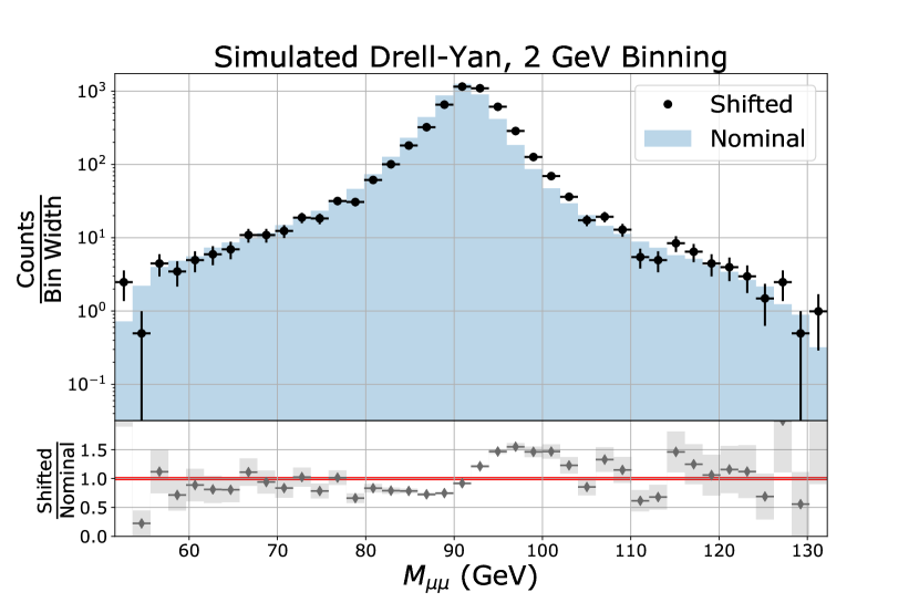
(a) Fixed-width binning.

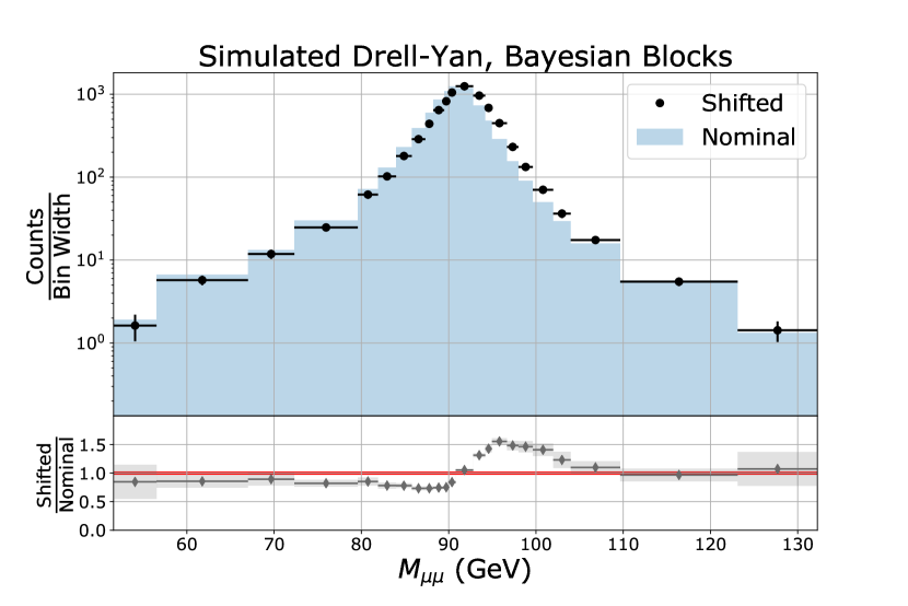
(b) Bayesian Block binning.

Figure 1: Comparison of simulated Drell-Yan distributions.

Our second illustration is the distribution of the transverse momentum $p_{T}$ of a reconstructed jet produced in association with a vector boson; this distribution is known to fall rapidly as $p_{T}$ increases and is characterized by a long, sparsely-populated, high-energy tail. High energy physicists will look for new physics in tails like this. Comparisons of data and Monte Carlo simulations can be unsatisfactory when a uniform binning is employed.

The two log plots in Fig. 2 show histograms produced with a typical 10 GeV binning and a binning determined by the Bayesian Blocks algorithm. The uniformly binned histogram is reasonable in the low-momentum region. However, it obscures an interesting minor disagreement between the data with the simulation that occurs in the lowest momentum region. Conversely, the high-momentum region is binned too finely, and the ratio plot (lower panel) in the lower panel is difficult to interpret due to large statistical uncertainties. The Bayesian Block histogram suffers from none of these defects, again producing a much more instructive and visually appealing plot. This distribution will also be examined quantitatively in the following section.

These two examples serve to showcase the Bayesian Block algorithm in realistic HEP plotting scenarios. Our statements thus far are qualitative and subjective in nature, as is typically the case when colloquially discussing the merits of data visualization methods. However, the following section will examine the Bayesian Block algorithm with a host of other common binning schemes in order to objectively compare and evaluate performance.

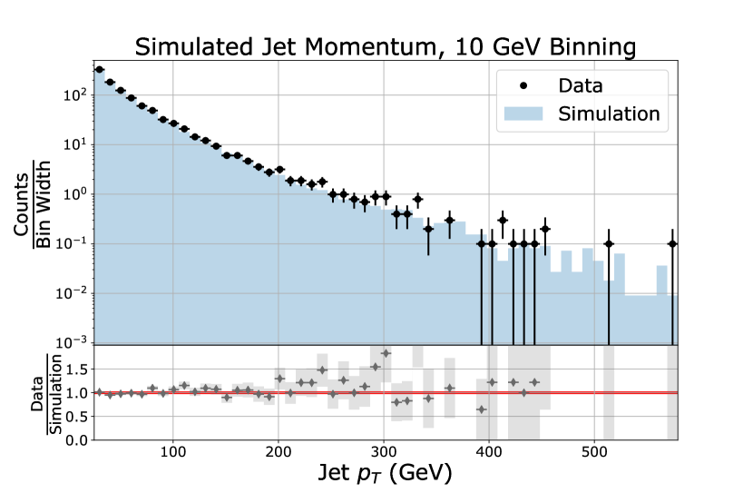
(a) Fixed-width binning.

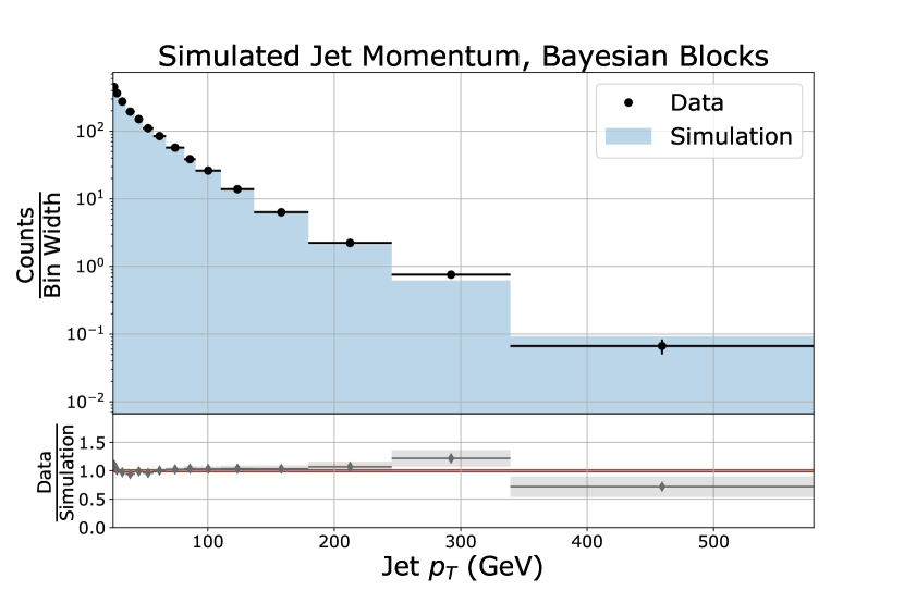
(b) Bayesian Block binning.

Figure 2: Comparison of simulated jet momentum distributions.

IV Comparison with Existing Methods

Many heuristics currently exist in order to generate an ‘optimal’ histogram, given an unbinned dataset. However, the criteria for determining which binning heuristic is optimal is not universally agreed upon. Scott Scott (1979) and others use the Integrated Mean Square Error (IMSE) to determine an optimal bin width. In practice, it is often difficult to obtain or approximate the underlying pdf for a given distribution, which is needed to calculate the IMSE. Additionally, the minimization of the IMSE does not take into account the visual appeal of the histogram to a user, which is an important, albeit difficult to quantify, aspect of data visualization.

In this section, we will compare multiple histogram binning methods with Bayesian Blocks, using metrics inspired by the studies conducted by Lolla and Hoberock Venu et al. (2011). These metrics will measure the visual appeal of a histogram and its ability to accurately reproduce the underlying pdf, without overemphasising statistical fluctuations inherent in any given dataset. The motivations and definitions of these metrics will be covered in Section IV.1.

We will evaluate the histograms using multiple different datasets with varying numbers of entries, motivated by distributions commonly seen in HEP. The two metric values will be displayed for all histogram methods employed for each example case, along with the final combined rank for each histogram method. The following histogram methods will be examined, along with the Bayesian Blocks algorithm:

1. Sturges Sturges (1926): $K=\lceil\ln(N)\rceil+1$.

2. Doane Doane (1976): Sturges rule, with a skewness correction.

3. Scott Scott (1979): $h=\frac{3.5\hat{\sigma}}{N^{1/2}}$, where $\hat{\sigma}$ is the standard deviation of the data.

4. Freedman-Diaconis Freedman and Daiconis (1981): $h=2\frac{\mathrm{IQR}i}{N^{1/3}}$, where IQR is the interquartile range of the data.

5. Knuth Knuth (2006): Fixed-width binning determined via likelihood minimization.

6. Rice Lane : $K=\lceil 2N^{1/3}\rceil$

7. Square root: $K=\lceil\sqrt{N}\rceil$

8. Equal population: Variable-width bins all contain equal number of entries.

IV.1 Histogram Metrics

Two metrics will be used to evaluate the performance of the histogram binning methods. The first metric is designed to capture the visual appeal of the histogram by minimizing the number of bin-to-bin height fluctuations. When dealing with a relatively smooth underlying distribution, these features, or “wiggles”, indicate that a histogram is picking up the unwanted statistical fluctuations inherent in a finite dataset. The number of wiggles in a histogram is defined as:

$$W_{n}=\sum[\operatorname{sgn}\left(f^{\prime}(B_{i})\right)\operatorname{sgn}\left(f^{\prime}(B_{i+1})\right)=-1]$$ (6)

where $f^{\prime}(B_{i})$ is the finite first derivative of the function describing the height of block (or bin) $i$. This metric simply counts the number of adjacent opposite-sign first derivatives, and increases when there are many fluctuations in height from one bin to another. A plot of $W_{n}$ as a function of the number of bins is shown in Fig. 3.

The second metric measures the accuracy of a given histogram in reconstructing the underlying pdf, while minimizing the impact of statistical fluctuations due to the initial data used to generate the histogram. Consider a dataset that consists of $N$ independent events, such that $D=\{d_{1},d_{2},d_{3},\ldots,d_{N}\}$. From dataset $D$, construct a histogram. From that histogram, generate a new set of data $\hat{D}=\{\hat{d}_{1},\hat{d}_{2},\hat{d}_{3},\ldots,\hat{d}_{N}\}$, where each data point is generated by a linear interpolation of each bin (e.g. for a bin ranging from 0 to 1 in x with height 5, we generate 5 equally spaced datum in x with values from 0 to 1.) This results in a set of data points equal in size to the original set, but evenly distributed within each respective bin. One can compare the interpolated dataset, $\hat{D}$ with $M$ different independent datasets, all of which are derived from the original distribution and have size $N$. We can use these datasets to construct the average error metric, defined as:

$$\hat{E}=\frac{1}{M}\sum_{m=1}^{M}\left(\sum_{n=1}^{N}|d_{nm}-\hat{d}_{n}|\right)$$ (7)

where $d_{nm}$ is the $n$th data point from the $m$th data set. This metric typically decreases as the size of the bins decrease, but in general does not approach 0 as the bins become infinitesimally narrow. The metric penalizes a histogram for modeling the statistical fluctuations of a given distribution by comparing the interpolated data with statistically independent datasets, and not the dataset used to generate the histogram. For the analyses performed in this manuscript, $M=100$ unless otherwise noted. A plot of $\hat{E}$ as a function of the number of bins is shown in figure 3.

There is no obvious way to combine metrics Eq. 6 and Eq. 7 to produce an overall metric. However, we will show the results of the metrics in a two dimensional plane, and also display the combined ranks of each histogram method. For nine different histogram methods, the best combined rank would be 2 (lowest relative score for each metric), and the worst combined rank would be 18 (highest relative score for each metric).

IV.2 Comparison Results

This section will show the outputs and metric results of histograms generated with the aforementioned binning heuristics for different distributions, and varying numbers of entries. The distributions examined are as follows:

1. A Drell-Yan invariant mass distribution (DY).

2. The transverse momentum of the leading muon from a Drell-Yan process (MuPT).

3. The transverse momentum of a jet produced in association with a vector boson (jPT).

4. A Gaussian distribution (Gauss).

5. A bimodal distribution formed from two Laplace distributions on a uniform background (2LP).

The DY, MuPT, and jPT distributions are all simulated using the Pythia and Delphes simulation software packages. The Gaussian and bimodal distributions are generated using the python package Numpy Jones et al. (01). Histograms are produced for each distribution with datasets of size $N$=500, 1000, 5000, and 10000. Both the Bayesian Block and equal population binning methods have a user-defined adjustable parameter. The Bayesian Blocks prior (Eq. 5) and the number of bins in the equal population method are determined by minimizing the combined metric ranks.

The histograms for the DY, MuPT, jPT, 2LP, and Gauss distributions are shown in Figs. 4-8. Plots of the two metrics, along with bar charts of the combined ranks of the metrics are shown in Figs. 9-13.

For the majority of the examples shown here, Bayesian Blocks outperforms the other binning methods in the context of the combined metric ranks. In almost every scenario, Bayesian Blocks is minimally wiggly, as the bin-to-bin statistical fluctuations are mitigated by the choice of bin width and edges. Infrequently, the Bayesian Block binning can produce a single “spike”, arising from a very narrow bin, which typically only occurs for relatively small datasets (see Fig.5 for $N$=500). This can be removed by tuning the prior, but at the cost of potentially increasing the overall coarseness of the binning. Typically, as the number of data points increases, the average error metric of Bayesian Blocks becomes competitive or surpasses the values associated with finer-binning methods. For some cases, notably the jPT and 2LP scenarios, Bayesian Blocks quickly becomes the objectively superior binning scheme with respect to both metrics. In general, as the size of the dataset increases, Bayesian Blocks approaches or arrives at the minima of $\hat{E}$ (with respect to other methods), without any signifiant increase in $W_{n}$. The decision of which binning heuristic to use for cases in which there is a relatively small dataset would depend on the personal preference of the user.

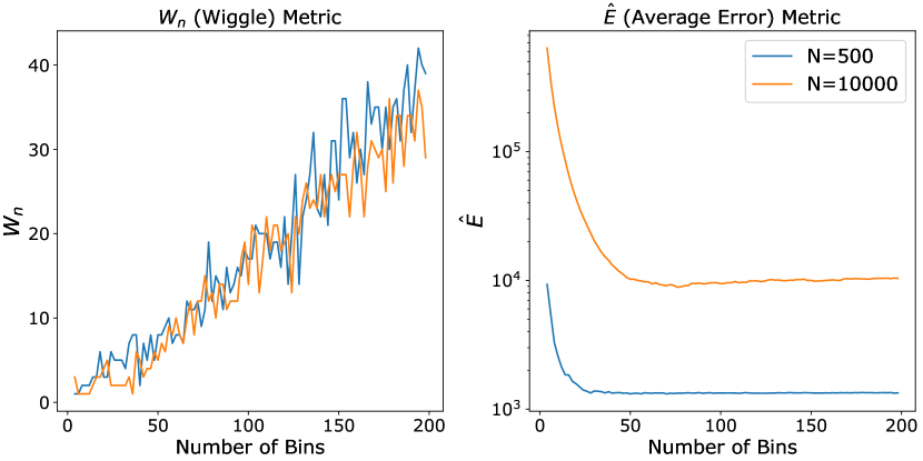
Figure 3: Metrics $W_{n}$ (left) and $\hat{E}$ (right) as a function of the number of (uniform width) bins. Distribution is jPT, for 500 and 10000 events.

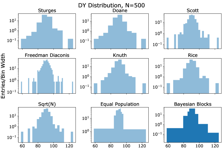
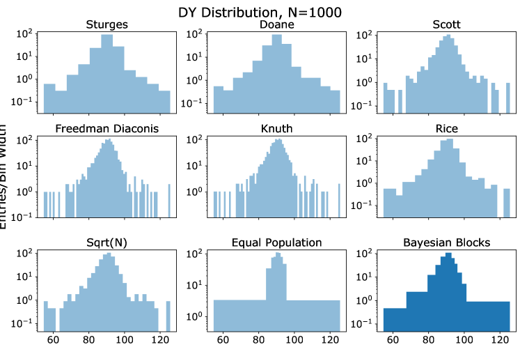
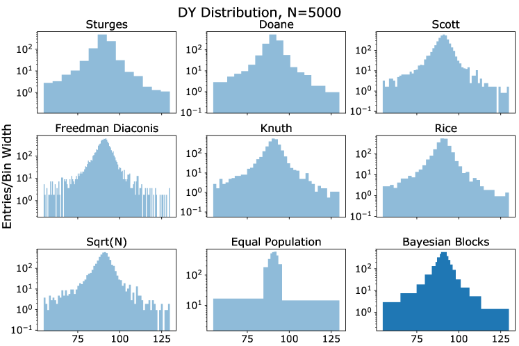
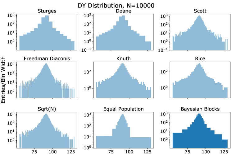
Figure 4: Histograms of Drell-Yan (DY) distribution for different sized datasets.

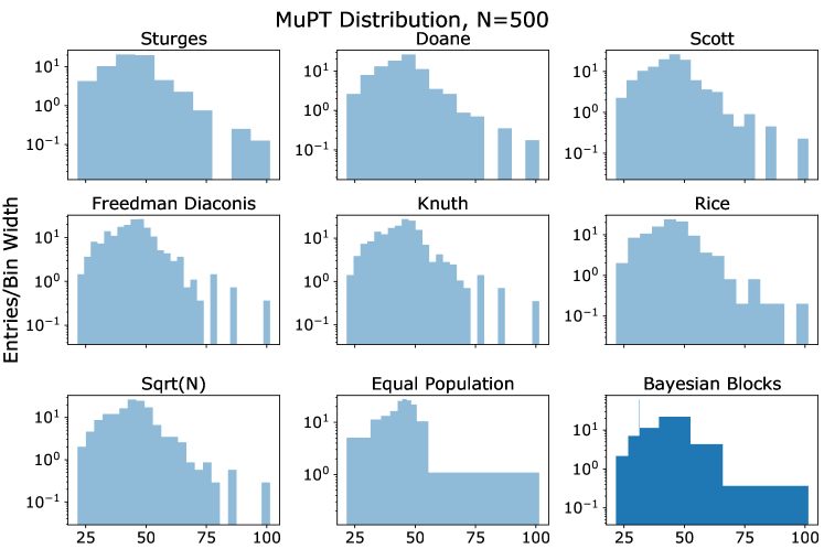
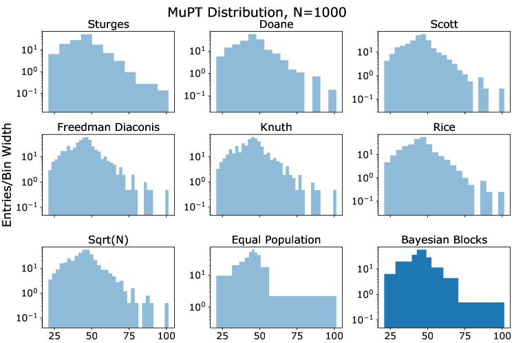
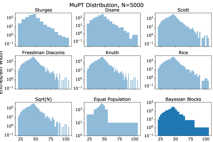
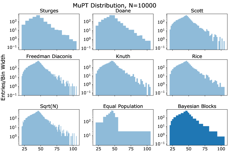
Figure 5: Histograms of muon transverse momentum (MuPT) for different sized datasets.

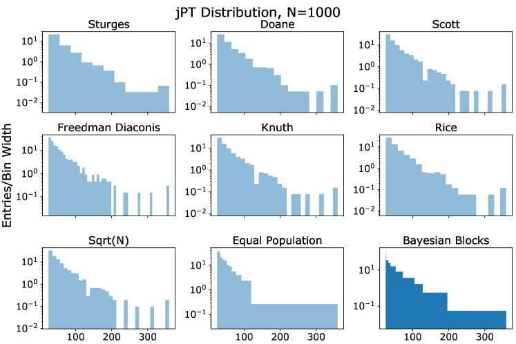
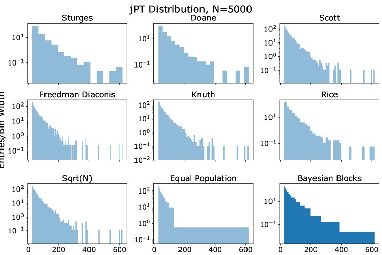
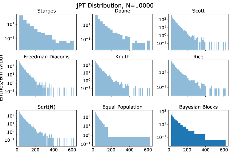
Figure 6: Histograms of jet transverse momentum (jPT) for different sized datasets.

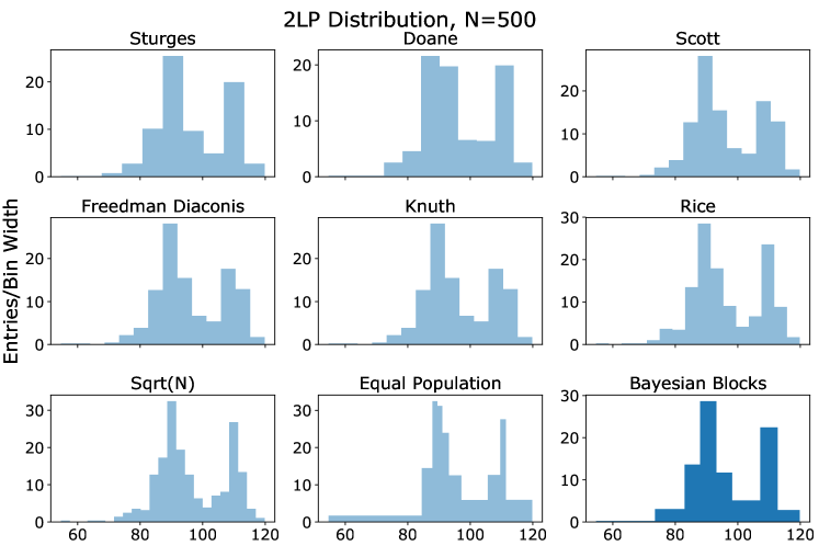
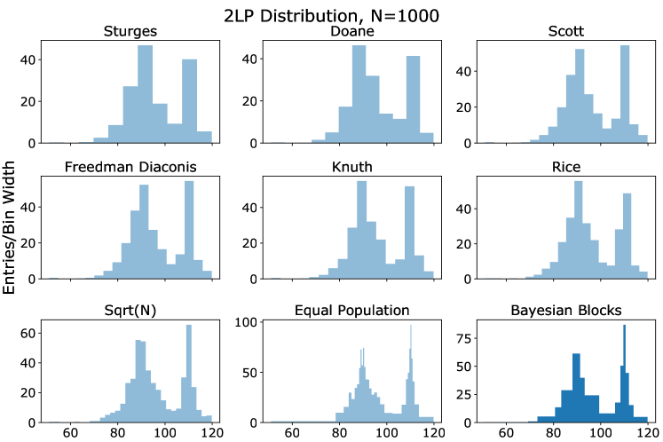
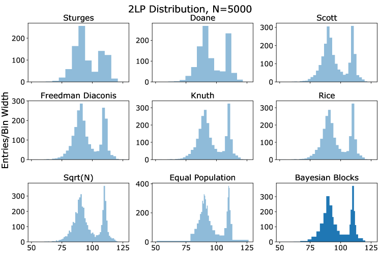
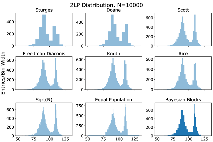
Figure 7: Histograms of a bimodal distribution (2LP) for different sized datasets.

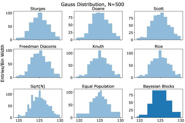
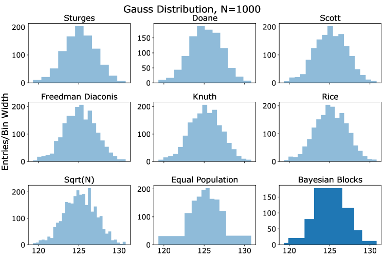
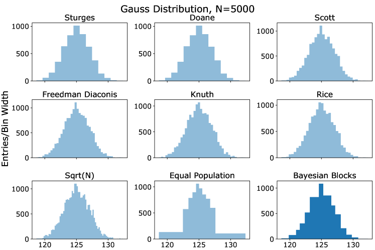
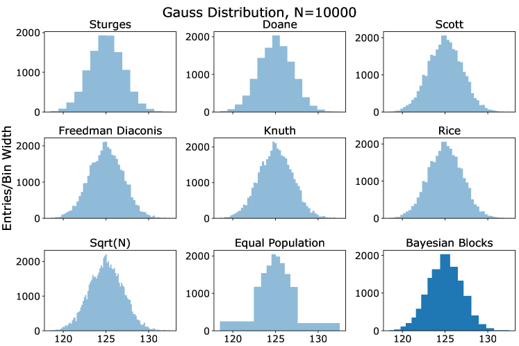
Figure 8: Histograms of Gaussian distribution (Gauss) for different sized datasets.

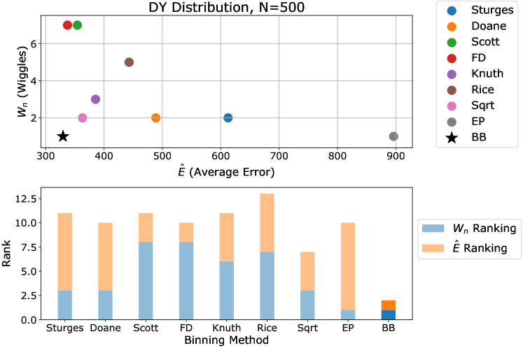
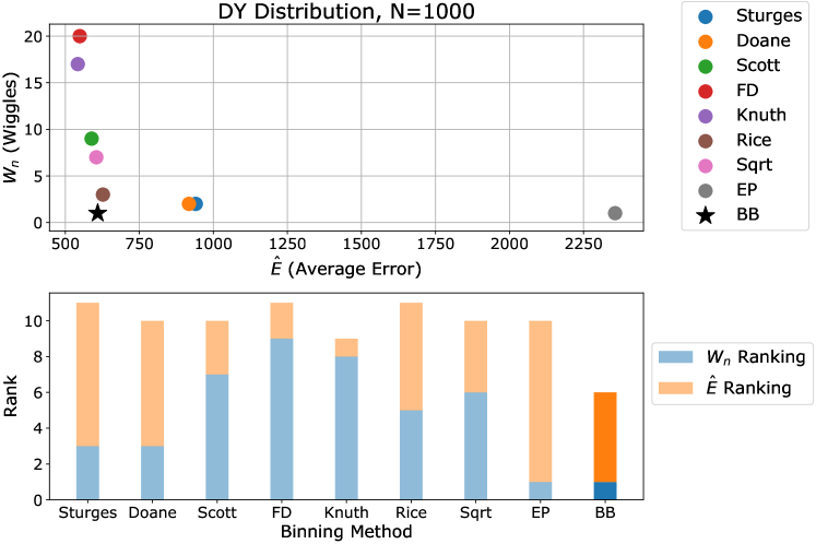
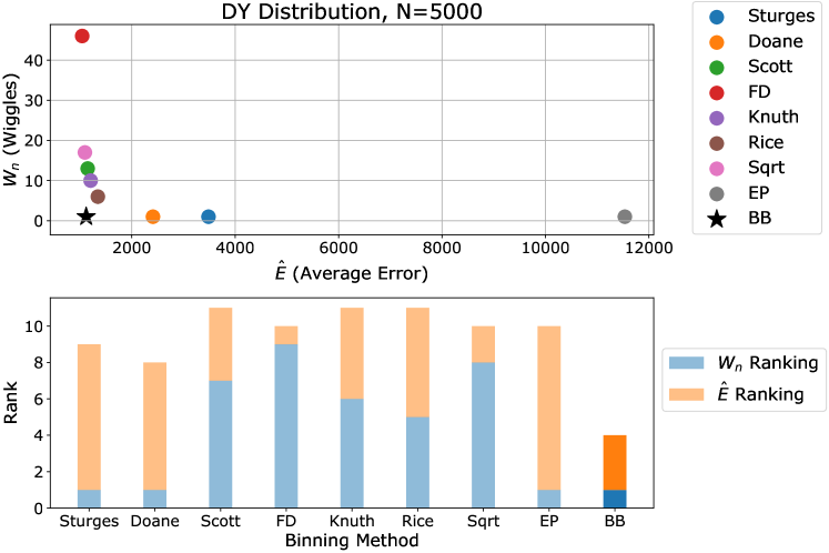
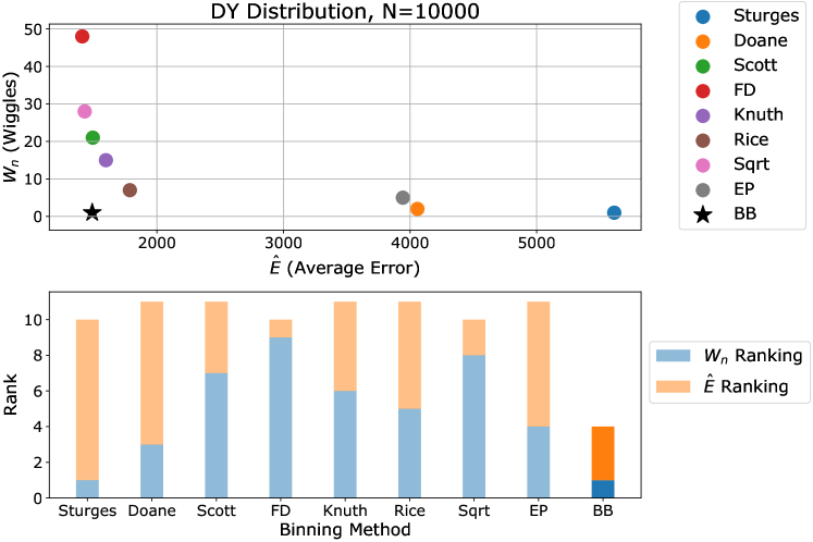
Figure 9: Metric values and combined ranks for Drell-Yan (DY) distribution for different sized datasets.

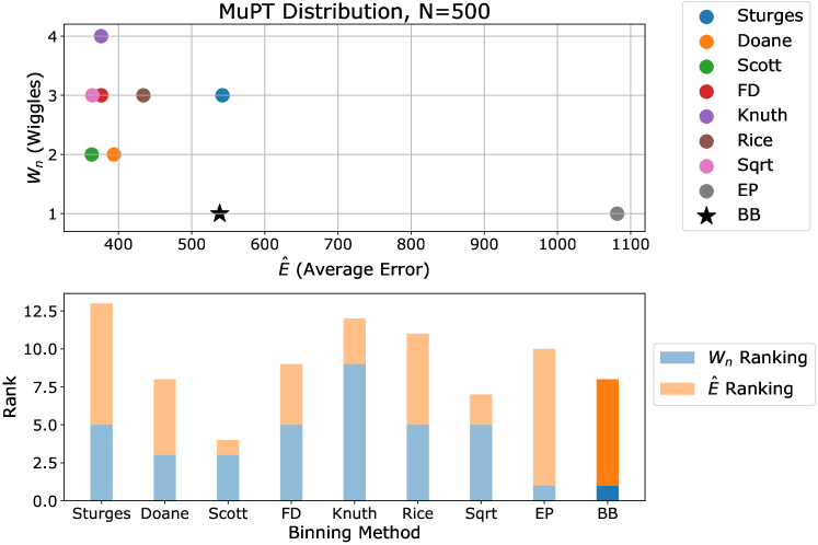
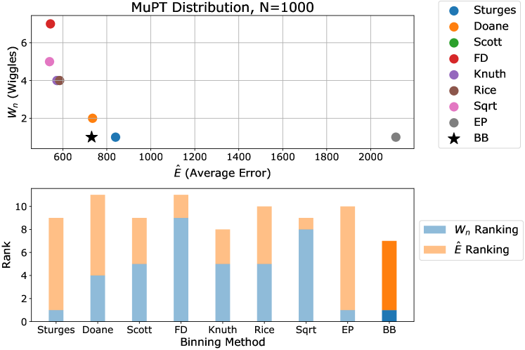
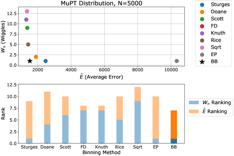
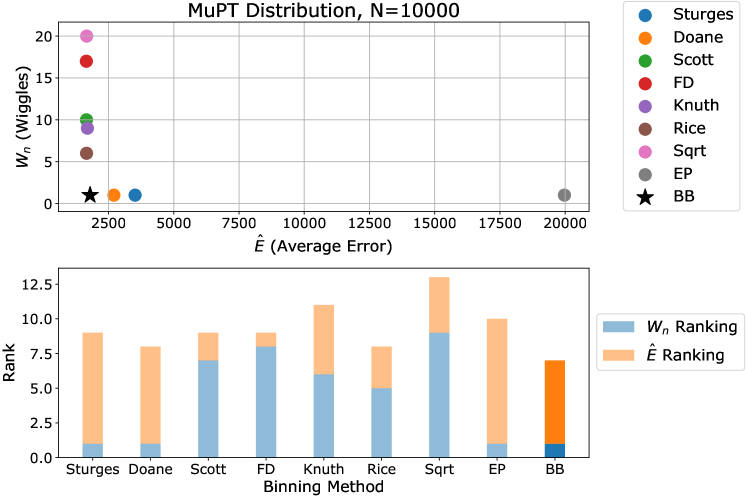
Figure 10: Metric values and combined ranks for muon transverse momentum (MuPT) for different sized datasets.

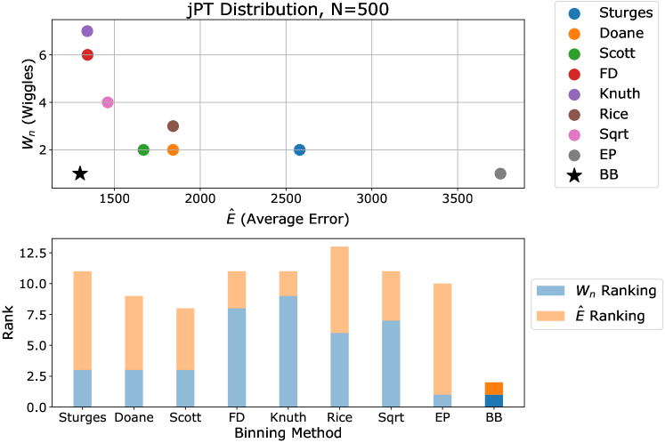
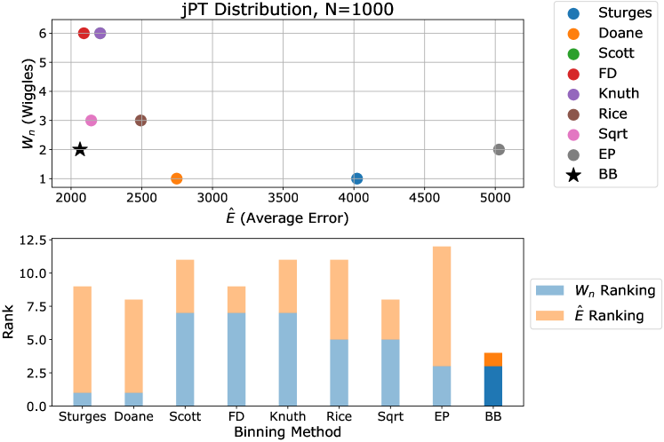
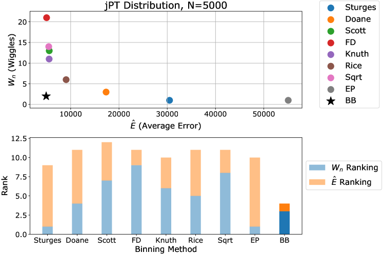
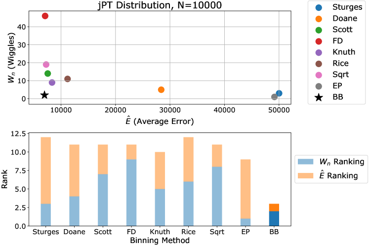
Figure 11: Metric values and combined ranks for jet transverse momentum (jPT) for different sized datasets.

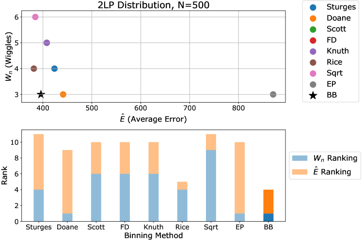
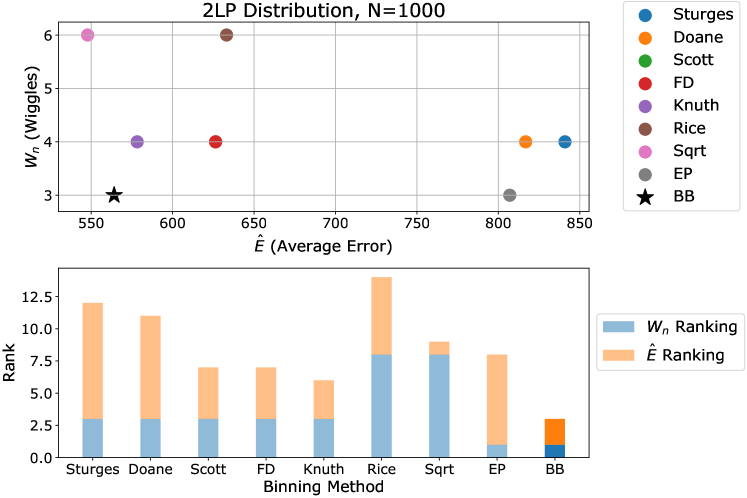
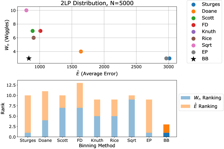
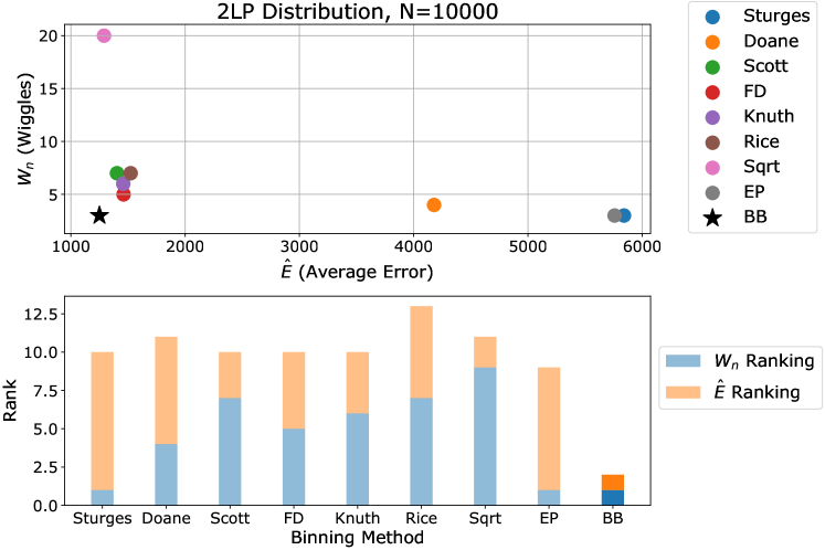
Figure 12: Metric values and combined ranks for a bimodal distribution (2LP) for different sized datasets.

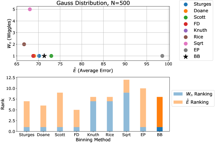
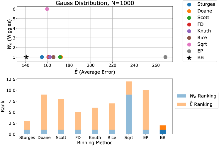
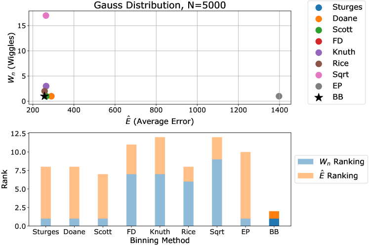
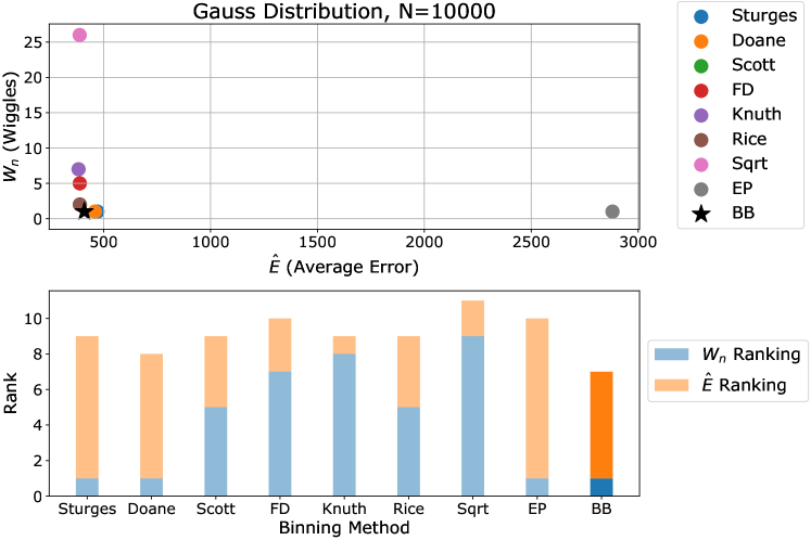
Figure 13: Metric values and combined ranks for Gaussian distribution (Gauss) for different sized datasets.

V Summary and Conclusions

We have shown that histograms specified with the Bayesian Blocks algorithm have certain advantages over typical histograms in high energy physics. First, the flexible binning allows for a better balance of statistical precision across a spectrum: sparse parts of distributions automatically have larger bins, and dense parts have smaller bins. Plots comparing two very similar distributions, especially the ratio of two similar distributions, are cleaner and easier to interpret, as illustrated by the plots in Figs. 1 and 2.

The benefits of the Bayesian Block algorithm are investigated quantitatively with respect to other popular binning schemes. We defined two metrics, $W_{n}$ and $\hat{E}$, to describe the visual appeal and the modeling accuracy of a given histogram. Given these metrics, and a host of distributions inspired by common HEP scenarios, the Bayesian Blocks algorithm proves to be a competitive or superior candidate, especially as size of the dataset increases. The binning it produces is extremely robust to statistical fluctuations, without sacrificing modeling accuracy. This makes Bayesian Blocks and ideal candidate for displaying and exploring data, without misleading the viewer with spurious bin-to-bin fluctuations or obscuring sharp features with excessively coarse binning.

This paper serves to introduce the Bayesian Blocks algorithm to the high energy physics community. Theoretical background can be found in the references, and applications await further data analysis elsewhere. The Bayesian Block implementation used in this paper can be found in the Scikit-HEP Rodrigues et al. (16) python package.