Squeezing the Efimov effect

Abstract

The quantum mechanical three-body problem is a source of continuing interest due to its complexity and not least due to the presence of fascinating solvable cases. The prime example is the Efimov effect where infinitely many bound states of identical bosons can arise at the threshold where the two-body problem has zero binding energy. An important aspect of the Efimov effect is the effect of spatial dimensionality; it has been observed in three dimensional systems, yet it is believed to be impossible in two dimensions. Using modern experimental techniques, it is possible to engineer trap geometry and thus address the intricate nature of quantum few-body physics as function of dimensionality. Here we present a framework for studying the three-body problem as one (continuously) changes the dimensionality of the system all the way from three, through two, and down to a single dimension. This is done by considering the Efimov favorable case of a mass-imbalanced system and with an external confinement provided by a typical experimental case with a (deformed) harmonic trap.

Introduction.

Few-body quantum systems are a theoretical and experimental playground for the study of the basic structure of quantum mechanics and what kind of states are possible in small systems, and they also serve as guidance when we want to understand many-body problems greene-review2017 ; naidon-review2017 ; zinner2014 ; dincao2017 . While the two-body problem is essentially solvable, at least numerically, three interacting quantum particles already provide a much more complex, and thus interesting, venue for exploration. A surprising feature is the Efimov class efi70 of infinitely many three-body bound states (trimers) of three bosons with resonant short-range two-body interactions in three dimensions (3D). This effect has generated tremendous attention in the last decade due to its observation in cold atoms kraemer2006 and lately in Helium trimers dorner2015 . The experimental techniques used to observe such states are extremely versatile with tunable interactions chin2010 geometries bloch2008 ; deng2016 , and usage of different atomic species gross2009 ; knoop2009 ; zaccanti2009 ; williams2009 ; gross2010 ; lompe2010 ; nakajima2010 ; berninger2011 ; machtey2012 ; wild2012 ; knoop2012 ; roy2013 ; dyke2013 ; huang2014 .

A prediction that has not yet been fully explored is the fact that the Efimov effect only occurs in 3D and not in 2D bruch1979 ; nielsen1997 ; brodsky2006 ; kartavtsev2006 ; pricoupenko2010 ; helfrich2011 ; volosniev2013 . (although one may find the so-called super-Efimov effect nishida2013 ; volosniev2014 ; gao2015 ; efremov2014 ) More precisely, by performing a well-defined mathematical extension to non-integer dimensions, it has been predicted that Efimov trimers of identical bosons are only allowed for dimension $d$ in the interval $2.3<d<3.8$ nie01 . This is a peculiar theoretical prediction that, superficially, appears basically inaccessible in actual experiments. On the other hand, non-integer dimensions play a prominent role in for instance high-energy physics schroder1995 and also in low-energy effective field theories valiente2012 , and it would be extremely useful to have a practical manner in which to study changes in dimensionality and how they affect basic quantum few-body physics.

The purpose of the present letter is to investigate how the energies of the Efimov states in 3D vary as functions of a continuously increasing confinement of the spatial dimensions imposed by external fields. The infinitely many 3D bound states reduce to a finite number in 2D, which may be reduced further as 1D is reached. This provides both qualitative and quantitative answers to the question of how much squeezing Efimov trimers can survive, as well as how trimers will disappear into the continuum. Some recent studies of Efimov trimers of three identical bosons under confinement have been reported lev14 ; yam15 , as well as earlier work on fermions in quasi-2D levinsen2009 and mixed-dimensional confinement nishida2008 . However, no previous study has been able to provide continuous dimensional squeezing from 3D to 2D, and all the way down to 1D with non-identical particles. Furthermore, the formalism we present can be applied to any confinement geometry in principle. Here we focus on the most widely applied experimental situation with a deformed harmonic confinement, and on mass asymmetric systems which are a current focus of three-body physics barontini2009 ; bloom2013 ; pires2014 ; tung2014 ; maier2015 ; ulmanis2016 ; wacker2016 ; johansen2016 .

Method.

We consider an $AAB$ system with two identical (bosonic) $A$ particles of mass $m_{A}$ and a $B$ of mass $m_{B}$. The reduced mass is defined by $\mu=m_{A}m_{B}/(m_{A}+m_{B})$. In order to reduce the number of parameters, we assume that the $A$ particles are not interacting, while the $AB$ subsystem has a short-range interaction that we model by a Gaussian potential, $-S_{0}\exp(-\bm{r}^{2}_{AB}/r_{0}^{2})$, where $\bm{r}_{AB}$ is the relative coordinate of the $AB$ system. The non-interacting nature of the $AA$ system is a matter of convenience and not essential as our formalism applies to general systems (see supmat for details). The interaction range, $r_{0}$, is kept small while the strength, $S_{0}>0$, is tuned so that it reproduces a fixed 3D (vacuum) scattering length, $a_{\textrm{3D}}$, in the region close to the resonance at $2\mu b^{2}S_{0}/\hbar^{2}=2.68$ where $|a_{\textrm{3D}}/b|=\infty$. For concreteness, we focus on the case where $a_{\textrm{3D}}>0$ so that a two-body bound state with small binding energy, $E_{2}^{\textrm{3D}}=\hbar^{2}/(2\mu a_{\textrm{3D}}^{2})$, exists. In order to squeeze the system, we assume the same external one-body harmonic oscillator potential on each particle along two directions, $\tfrac{1}{2}m(\omega_{x}^{2}x^{2}+\omega_{y}^{2}y^{2})$, where $m$, $x$ and $y$ are mass and single-particle Cartesian coordinates of particles $A$ or $B$. For simplicity we use identical external confinement on each particle as this decouples the center-of-mass motion supmat . We expect the physics to remain qualitatively the same with unequal trapping. Defining $b_{x}=\sqrt{\hbar/\mu\omega_{x}}$ and $b_{y}=\sqrt{\hbar/\mu\omega_{y}}$, we squeeze the system starting from large values of $b_{x}$ or $b_{y}$ and decreasing these towards $b_{x}\to 0$ or $b_{y}\to 0$.

In order to solve the three-body problem we use a momentum-space approach and the integral Faddeev equations adh95a ; adh95b ; fre11 . These equations are modified to allow for squeezing by imposing periodic boundary conditions along one or several directions, effectively compactifying those dimensions on a ring of radius $R_{x/y}$. This implies that the momenta along the compact directions are discrete. In the limit where $R_{x/y}\to 0$, the gap in the spectrum along a compact dimension goes to infinity, which eliminates motion in that direction, whereas in the limit $R_{x/y}\to\infty$, the gap vanishes and we recover the usual continuous spatial $x/y$ dimension. The results presented in this letter show that this formalism is capable of addressing the full crossover between different (integer) dimensions for general three-body systems of any mass.

The concrete implementation of our compactified Faddeev equations uses effective zero-range interactions. However, as is well-known from previous three-body Efimov studies efi70 , the decisive parameter(s) are the two-body binding energies between pairs of particles, which are typically parameterized by $a_{3D}$. In our setup, we have $AB$ interactions with two-body energy $E_{2}^{\textrm{3D}}$. It is important to stress that our input is the two-body energy calculated in a fully 3D setup that includes the external confinement. This is done by calculating $E_{2}^{\textrm{3D}}$ using a correlated Gaussian numerical technique mitroy2013 with fixed $a_{\textrm{3D}}$ while varying the trap by decreasing for instance $b_{y}$. We then relate $b_{y}$ and $R_{y}$ by demanding that $E_{2}^{\textrm{3D}}(b_{y})=E_{2}^{\textrm{3D}}(R_{y})$, where the latter is calculated with a compact dimension (see supmat for details). Numerically, we find the remarkably simple result $b_{y}\approx 2\pi R_{y}$, and clearly see that $b_{y}\to 0$ will correspond to the 2D limit as expected. Further squeezing from 2D down to 1D is accomplished by starting from a 2D version of the Faddeev equations bel11 ; bel12 ; bel13b and is otherwise analogous supmat . This method can be extended to other kinds of confinement through the two-body subsystems.

Two-body properties.

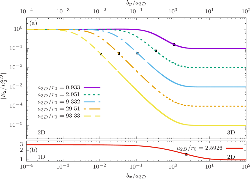
We first consider the $AB$ two-body subsystem. The energy as function of $b_{y}/a_{\textrm{3D}}$ for fixed $a_{\textrm{3D}}$ is shown in Fig. 1(a) where we have normalized to the energy in the 2D limit ($b_{y}\to 0$). In Fig. 1(a) we see an evolution from the 3D limit (far right side) with energies that remain constant until around the point where $b_{y}\sim r_{0}$. This is when the external confinement starts to be felt strongly by the particles and the energy moves quite fast towards the 2D limiting value. It is interesting to note that the energy at which $b_{y}=r_{0}$ (marked by black points in Fig. 1) is almost the same, $E_{2}/E_{2}^{\textrm{2D}}(b_{y}=r_{0})\sim 0.05$, independent of $a_{\textrm{3D}}$ for $a_{\textrm{3D}}/r_{0}\gg 1$. The evolution from 2D to 1D is shown in Fig. 1(b) and confirms our expectation that further binding occurs as we approach the 1D limit.

Figure 1: (a) The two-body energies normalized to the 2D limit ($E_{2}^{2D}$) as functions of $b_{y}/a_{3D}$ for different $a_{3D}/r_{0}$. The black points indicate where $b_{y}=r_{0}$. (b) The corresponding 2D to 1D transition as function of $b_{x}/a_{3D}$. The length scale $a_{2D}$ is defined through $|E_{2}^{2D}|=4e^{-2\gamma}\hbar^{2}(\mu a_{2D}^{2})^{-2}$, where $\gamma$ is Euler’s constant.

Spectral flow from 3D to 2D.

We now proceed to discuss Efimov trimer states as we continuously squeeze along one direction, i.e. as $b_{y}$ decreases. The mass ratio is taken to be $m_{B}/m_{A}=6/133$ note-on-dim and is relevant for current studies of trimers in ⁶Li-¹³³Cs mixtures pires2014 ; tung2014 ; ulmanis2016 ; johansen2016 . This gives a relatively small Efimov scaling factor $e^{\pi/s}=4.788$ jen03 ; yam13 so that many Efimov trimers can be expected. We choose a large $a_{\textrm{3D}}/r_{0}\simeq 10^{5}$ to perform our calculations.

Figure 2: Trimer energies plotted in units of the two-body energy for $m_{B}/m_{A}=6/133$ as functions of $b_{y}/a_{\textrm{3D}}$. For the solid lines the two-body energy varies with $b_{y}$ while for the dashed lines it is kept constant (see text for discussion). Solid and dashed lines have different colors for visibility.

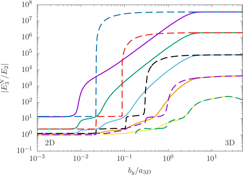
The three-body energies of the $N$th trimer, $E_{3}^{N}$, relative to the two-body energy are shown in Fig. 2 as function of $b_{y}/a_{\textrm{3D}}$. In the 3D limit to the far right, we are able to numerically resolve five Efimov states which scale in energy with $e^{2\pi/s}$ as expected. In the strict 2D limit on the far left of Fig. 2, we find that four states survive as expected bel11 . The behavior in between these two integer limits is intriguing and depends sensitively on how we treat the two-body energy.

The dashed lines in Fig. 2 show the results obtained when assuming that the two-body energy does not vary with $b_{y}$ and is set by the 3D value, $E_{2}=E_{2}^{\textrm{3D}}(b_{y}\to\infty)$. As $b_{y}$ decreases we see a number of systematically occurring abrupt drops in $E_{3}^{N}$. Each drop is from an initial value down to one of the energies that the system is destined to reach in 2D where the Efimov effect is gone.

Specifically, as we decrease $b_{y}$ (going from right to left in Fig. 2) the state that is weakest bound in the 3D limit first decreases its energy to a value corresponding to the strongest bound state in the 2D limit. It then has roughly constant energy until the next level decreases its energy and demands the position in the spectrum, and pushed the state down to an energy around that of the first excited state in the 2D limit. These processes are repeated until the four 2D positions are reached and the remaining three-body state has disappeared into the continuum (a single state in our case). They are reminiscent of the so-called Zeldovich rearrangement zeldovich1960 , in which the short-range interactions compete with the long-range influence of the confinement.

It is important to notice that before these abrupt changes of the energies, the Efimov scaling among the states is intact. Thus, we have a quantitative measure of how much squeezing different Efimov states can survive. A rough estimate of the jumps can be inferred by considering the Efimov attractive inverse square potential which extends to around $a_{\textrm{3D}}$ jensen2004 ; braaten2006 , and therefore the radial extent of the least bound state is roughly $a_{\textrm{3D}}$. In turn, the first spectral jump is expected around $b_{y}\sim a_{\textrm{3D}}$, since here the state becomes strongly influenced by the trap portegies2011 . Subsequent jumps now follow an Efimov scaling law and occur when $b_{y}\sim a_{\textrm{3D}}/e^{N\pi/s}$.

Keeping a constant $E_{2}$ value is presumably experimentally challenging as it requires tuning of interactions to compensate for the effects of the confinement on $E_{2}$. We therefore now study the case where this is not done so that we now have a varying $E_{2}(b_{y})$. This changes the flow as seen in Fig. 2. The decrease of energies will start for larger values of $b_{y}$ and have a considerably smoother behavior. Remarkably, we see that the energy curves are roughly parallel on a double-log scale, thus showing that even in this case we have signatures of Efimov scaling prominently featured. We stress that, even though the abrupt changes found for a constant $E_{2}$ are now smoother, we still clearly see the rearrangements discussed above, and these features could be a very clear experimental signature to confirm the present predictions.

Figure 3: Energies as in Fig. 2 but now multiplied by the scaling factor $\exp(2\pi N/s)=22.92^{N}$ where $N=0,1,2,3,4$ for ground and excited states.

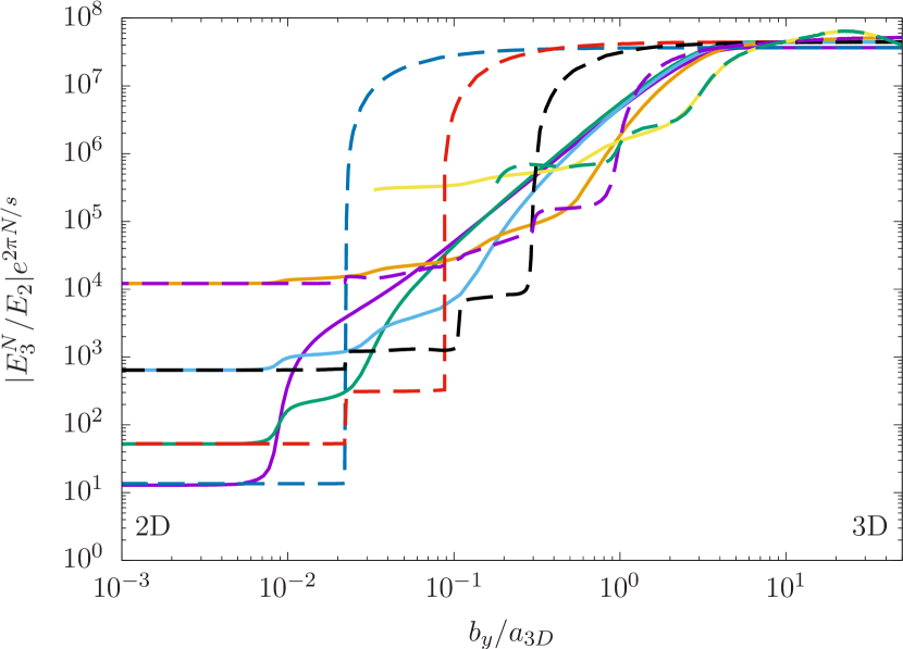
In order to investigate the Efimov scaling as function of the squeezing, we now multiply the three-body energies by $e^{2\pi N/s}$ for the $N$th Efimov state in the energies. The results are shown in Fig. 3. For the case of constant $E_{2}$ the results are very similar to Fig. 2, while those with varying $E_{2}(b_{y})$ now more clearly shows a tendency to collapse onto a single curve over an extended region. This region is limited by the necessity for the states to match up with their 2D limiting values, and they each leave the common curve due to rearrangements one at a time starting from the weaker bound state. We can infer from the dashed lines in Fig. 3 that a scaling of $e^{2\pi N/s}$ on $b_{y}$ would tend to also collapse the case of constant $E_{2}$ onto a single curve. This is not needed when $E_{2}$ varies. The intriguing conclusion appears to be that the two-body subsystem ($E_{2}(b_{y})$) already contains the information on the scaling.

Squeezing down to 1D.

Starting from the 2D limit results shown in Fig. 2, we may consider what happens as we further squeeze the system down to 1D by increasing the harmonic confinement along the $x$-direction. Technically, we start from 2D Faddeev equations and proceed as before (see supmat for details). The results of this are shown in Fig. 4. We notice similar behavior with plateaus in 2D and 1D limits connected by intermediate transitions where the energy changes rapidly. Notice that for the mass ratio used, the 1D limit only holds three bound states, and one state goes to the continuum during the dimensional reduction.

Figure 4: The ratio of three- and two-body energies for $m_{B}/m_{A}=6/133$ as functions of $b_{x}/R_{rms}^{N}$. The dashed curves for all states are with $R_{rms}=R_{rms}^{0}=0.4742b=0.2101\hbar/\sqrt{m_{A}E_{AB}(2D)}$ (see text for discussion). Solid and dashed lines differ in color for visibility.

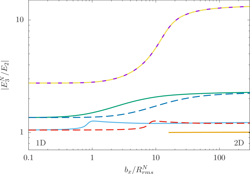
As Efimov scaling does not extend to these low dimensions, the natural quantities to analyze the system are slightly different. As was recently discussed in Ref. san16 , the root-mean-square radius of the $N$th $2D$ three-body state, $R_{rms}^{N}$, is proportional to the inverse square root of $E_{2}^{\textrm{2D}}$, with a proportionality factor that depends on the state index $N$ and the mass ratio. Since the three-body equations depend only on the quantity $E_{2}(b_{x})$ supmat , the three-body energy must be a function of $E_{2}(b_{x})$. In turn, the three-body to two-body energy ratio will depend only on $b_{x}/R_{rms}^{N}$ for the $N$th state. The transition from 2D to 1D can therefore be studied in a universal manner by using this variable as done in Fig. 4. For comparison, we plot the energies as function of $b_{x}/R_{rms}^{0}$ with dashed lines in Fig. 4, in order to follow each state for the same value of $b_{x}$.

The bound state behavior under squeezing from 2D to 1D is clearly different from the case of 3D to 2D. In particular, we see in Fig. 4 that all the three states that survive to the 1D limit start to feel the squeezing already for relatively large traps. If we focus on the dashed lines, we see that the center of the drop is around $b_{x}/R_{rms}^{0}\sim 10$ for all of the states, indicating that we have a synchronized pattern of rearrangements in contrast to the hierarchical pattern seen in Fig. 2 and Fig. 3. In Fig. 4, the stronger bound state gets pushed to its 1D limit and forces the other states to follow suit. However, it is still very clear that there is a sizable effect of the squeezing that should be observable.

Experimental implications and outlook.

Observing the influence of squeezing on the Efimov effect and the spectral flows that this generates should be possible with the experimental techniques that have hitherto been used to probe three-body physics with cold atoms. A much used tool is recombination rate studies where three-body states are identified by peaks and interference minima in the rate. In the case of squeezing from 3D to 2D, we have a finite $b_{y}$. We may now vary $a_{\textrm{3D}}$ while keeping $b_{y}$ fixed which will scan from right to left in Fig. 2, and would expect to see a feature in the recombination rate around the point where the least bound state enters the continuum. Here we use that the flow depends solely on $b_{y}/a_{\textrm{3D}}$, but we note that the number of bound states to work with depends on how large initial value of $a_{\textrm{3D}}$ one can access in a concrete experiment. Similarly, if we consider an experiment where $b_{y}$ is tuned independently of $a_{\textrm{3D}}$, then we may take a fixed ratio $b_{y}/a_{\textrm{3D}}$ and vary $a_{\textrm{3D}}$ which will cause bound states to cross into the continuum. Doing so for several different values of $b_{y}/a_{\textrm{3D}}$ would allow verification of our predictions. The same method can be applied in the case where we go from 2D to 1D. An alternative to recombination rate measurement is to use radio frequency association lompe2010 ; nakajima2010 to access the binding energies themselves. This is more difficult but also yields more information. In this case one should be able to observe the spectrum at several points by varying $b_{y}$ and/or $a_{\textrm{3D}}$ to see the flow of the states.

Outlook.

In the present work we have focused our attention on a simple setup in order to best illustrate the effects of squeezing on the energies of Efimov trimers. Our formalism can be used to discuss other quantities such as radial extension of states, momentum distributions etc. We have also chosen a particular mass ratio that corresponds to recent experiments, but simplified our discussion by neglecting interactions between the two heavy particles in the trimer. While we do expect quantitative changes when including this interaction, the qualitative behavior should be the same. Likewise, we expect the same behavior as discussed here in the case where $a_{3D}$ is large but with negative sign. A cylindrical confinement may also be accommodated by a simple modification of our formalism and this will allow squeezing of the system along two directions ($b_{x}=b_{y}\to 0$). Initial investigations indicate that a direct transition from 3D to 1D yields similar results to those presented above.

Acknowledgments.

The authors would like to thank A. R. Rocha, S. J. J. M. F. Kokkelmans, and J. Levinsen for feedback on the results and the manuscript. This work was partly supported by funds provided by the Brazilian agencies Fundação de Amparo à Pesquisa do Estado de São Paulo - FAPESP grant no. 2016/01816-2(MTY), Conselho Nacional de Desenvolvimento Científico e Tecnológico - CNPq grant no. 302075/2016-0(MTY), Coordenação de Aperfeiçoamento de Pessoal de Nível Superior - CAPES no. 88881.030363/2013-01(MTY), and by the Danish Agency for Science, Technology, and Innovation.

Supplemental Material for “Squeezing the Efimov Effect”

I Squeezed dimer

In this section we present the equations that are used to obtain the dimer energy as we squeeze along one (3D$\rightarrow$2D) or along two (2D$\rightarrow$1D) spatial dimensions. We will be using units where $\hbar=1$ throughout the discussion in this supplementary material.

I.1 Transition from 3D$\rightarrow$2D

In our model we will assume periodic boundary conditions along one direction (chosen to be the $y$-axis). Then, the relative momenta along the plane are given by $\vec{p}_{\perp}=(p_{x},p_{z})$ and

$$p_{y}=\frac{n}{R_{y}}\ ,$$ (1)

with $n=0,\pm 1,\pm 2,\dots$. The length of the squeezed dimension corresponds to a radius, $R_{y}$, that interpolates between the 2D limit for $R_{y}\to 0$ and the 3D limit for $R_{y}\to\infty$. As discussed in the main text, the choice of a periodic dimension is not essential for our study, as we may map the physics of other types of external confinement onto the system with periodic boundary conditions. In the present case we consider the case of a harmonic oscillator confinement that we map onto the periodic setup.

First, we consider the case where we have zero-range (ZR) interactions. In general, the dimer energy with zero-range interactions $E_{2}^{ZR}$ is a function of $R_{y}$. A natural fixed point of the dimer energy is the 3D limit where the shallow zero-range dimer energy around for instance a Feshbach resonance is experimentally measurable. We denote this dimer energy of a 3D setup (no squeeze) by $E_{2}^{3D}$. This implies that the two-body $T$-operator in the limit $R_{y}\to\infty$ has to recover a pole exactly at $E_{2}^{3D}$. Thus, for the zero-range potential we must solve ziegelmann

$$\int d^{3}p\frac{1}{E_{2}^{3D}-\frac{p^{2}}{2M}}-\frac{1}{R_{y}}\sum_{n}\int d^{2}p_{\perp}\frac{1}{E_{2}^{ZR}-\frac{p_{\perp}^{2}}{2M}-\frac{n^{2}}{2MR_{y}^{2}}}=0\ ,$$ (2)

where $M$ is the reduced mass of the dimer. The above equation can be solved analytically giving:

$$\sqrt{-ME_{2}^{ZR}}=\frac{1}{\pi R_{y}}\sinh^{-1}\frac{e^{\pi\,R_{y}/a_{3D}}}{2}\ ,$$ (3)

where $a_{3D}=\sqrt{-E_{2}^{3D}}$ is the two-body scattering length. The explicit form of (3) reads:

$$E_{2}^{ZR}=-\frac{a_{3D}^{2}}{(\pi R_{y})^{2}}\ln^{2}\left(\frac{e^{\pi\,R_{y}/a_{3D}}}{2}+\sqrt{\frac{e^{2\pi\,R_{y}/a_{3D}}}{4}+1}\right)\ ,$$ (4)

and for $R_{y}\to 0$ one has that, for a zero-range potential, the dimer energy changes as:

$$E^{ZR}_{2}\sim-(\pi MR_{y})^{-2}\,(\sinh^{-1}\frac{1}{2})^{2}=0.02346227\,\,(MR_{y})^{-2}.$$ (5)

This result should not be valid for a finite-range potential, as in this case we expect a finite dimer energy when the system is confined in two dimensions ($R_{y}\to 0$).

The argument above shows that the route toward $R_{y}\to 0$ depends on the form of the two-body potential. In order to regularize $E^{ZR}_{2}$ for $R_{y}\to 0$, we assume a simple fitting formula for the dimer energy as a function of $R_{y}$. This formula will have two parameters constrained to the dimer binding energies calculated numerically at the 2D and 3D limits as we will now discuss.

To calibrate the zero-range model, we use the numerically highly robust stochastic variational method to calculate the dimer binding energies in the presence of a harmonic trap which is then squeezed along one direction. The zero-range interaction is modeled by a Gaussian two-body potential. Thus, we solve the following eigenvalue equation

$$H|\Psi\rangle=\left(\frac{p_{AB}^{2}}{2M}+V(r_{AB})+\frac{M}{2}\left(\omega_{x}^{2}x_{AB}^{2}+\omega_{y}^{2}y_{AB}^{2}\right)\right)|\Psi\rangle\,=\,e_{2}|\Psi\rangle\,,$$ (6)

where $V(r)=S_{0}e^{-r_{AB}^{2}/r_{0}^{2}}$ is the two-body interaction at (relative) distance $r_{AB}$ with strength $S_{0}$ and range $r_{0}$. When we squeeze from 3D to 2D, we take $\omega_{x}=0$ and increase $\omega_{y}$. Note that $x_{AB}$ and $y_{AB}$ are the Cartesian components of the relative distance between the two particles, $r_{AB}$. The center of mass part of the trap decouples from the problem and can be ignored in our case where we are only interested in the intrinsic internal dynamics of dimer and trimer states. The energy $e_{2}=\frac{\langle\Psi|H|\Psi\rangle}{\langle\Psi|\Psi\rangle}$ is calculated from a correlated Gaussian basis used to expand the wave function suzuki .

Equation (6) is now used to define $E_{2}(\omega_{y})=e_{2}-\frac{\hbar\omega_{y}}{2}$. The subtraction of the zero-point contribution is important as one would otherwise get a divergent contribution that would reflect only the increasing trap energy and not the intrinsic behavior of the dimer. We find that the dimer energy is accurately described by the form

$$E_{2}(b_{y})=-\frac{4a_{3D}^{2}}{\alpha+\beta b_{y}^{2}}\ln^{2}\left(\frac{e^{b_{y}/2a_{3D}}}{2}+\sqrt{\frac{e^{b_{y}/a_{3D}}}{4}+1}\right),$$ (7)

where we have defined the oscillator length $b_{y}=\sqrt{1/M\omega_{y}}$. This form is of course inspired by the zero-range dimer energy above, Eq. (4). In order to fix the parameters, $\alpha$ and $\beta$, we may use the limiting expressions $E_{2}(b_{\omega}\to 0)\equiv E_{2}^{2D}$ and $E_{2}(b_{\omega}\to\infty)\equiv E_{2}^{3D}$, which gives

$$\alpha\equiv-\frac{4a_{3D}^{2}}{E_{2}^{2D}}\ln^{2}\left(\frac{1+\sqrt{5}}{2}\right)\,{\rm and}\,\beta\equiv-\frac{1}{E_{2}^{3D}}.$$ (8)

By comparison between Eq. (4) and Eq. (7), we may now infer that the mapping between our setup with periodic boundaries to that of the harmonic trap is obtained by identifying $2\pi R_{y}=b_{y}$. Numerically, we find that this relationship is extremely accurate.

The procedure above may be performed for other confinement potentials with little extra complication as the stochastic variational method is highly flexible mitroy2013 and can provide the necessary dimer energies that we need to calibrate our setup with zero-range interactions and periodic boundaries. The precise mapping relation between $R_{y}$ and the length parameters of other confining potentials may of course differ from that presented here.

I.2 Transition 2D$\rightarrow$1D

In this section we squeeze one of the two remaining directions of the last subsection confining the dimer in 1D. This corresponds to now increasing $\omega_{x}$. We repeat essentially the same steps to obtain the binding energy of the dimer as a function of $R_{x}$. Eq. (2) is changed so that it describes the $2D\to 1D$ transition. In this case it has the form

$$\int\frac{d^{2}p}{E_{2}^{2D}-\frac{p^{2}}{2M}}-\frac{1}{R}_{x}\sum_{n}\int\frac{dp}{\bar{E}_{2}-\frac{p^{2}}{2M}-\frac{n^{2}}{2MR_{x}^{2}}}=0,$$ (9)

where the two-body binding energy is written with a bar $\bar{E}_{2}$ and now depends implicitly on $R_{x}$. After performing the sum over the discrete modes and the integration over one of the momenta, we get the following transcendental equation for the two-body binding energy as:

$$\ln\left(\frac{\bar{E}_{2}}{E_{2}^{2D}}\right)=2\int^{\infty}_{0}dp\frac{\coth(\pi\,R_{x}\sqrt{-\bar{E}_{2}+p^{2}/2M})-1}{\sqrt{-\bar{E}_{2}+p^{2}/2M}}\ .$$ (10)

In the limit $R_{x}\to\infty$, Eq. (10) reproduces the two-body energy in $2D$. However, it diverges in the limit $R_{x}\to 0$ and needs to be regularized. This is done by replacing $R_{x}^{2}\to R_{x}^{2}+R_{0}^{2}$, in which $R_{0}$ is an adjustable parameter that allows us to obtain $\bar{E}_{2}(R_{x}=0)=E_{2}^{1D}$, where $E_{2}^{1D}$ is the two-body energy in $1D$ which is calculated via the the stochastic variational method using a Gaussian potential just as we have done in the previous section. The mapping is again found to be $2\pi R_{x}\approx b_{x}$, where $b_{x}=\sqrt{1/M\omega_{x}}$.

II Squeezed trimer

The trimer we now consider is an $AAB$ system with two identical $A$ particles of bosonic kind, and a third particle $B$ that may have a different mass. In what follows we detail the integral equations for the bound state, in which we introduce a compact dimension through a periodic boundary condition quantizing the relative momentum of the third particle with respect to the interacting pair. Furthermore the two-body amplitudes for a given squeezing situation are defined such that the two-body bound state energies come from Eqs. (7) and (10) for the transition 3D$\to$2D and 2D$\to$1D, respectively.

II.1 Transition 3D$\rightarrow$2D

To describe the trimer, we will use relative Jacobi coordinates, where $\vec{p}$ represents the relative momentum of a given pair of particles in the three-body system and $\vec{q}$ the momentum of the remaining particle with respect to center of mass of said pair. We are interested in the universal limit where the ranges of all two-body interactions can be neglected. This means that we consider zero-range interaction as in the dimer case above. Zero-range interactions present a singularity which is resolved by a subtraction in the kernel with the introduction of a scale, $\mu^{2}$ adhikari . For simplicity we will use units where $\hbar=m_{A}=1$ from now on and introduce the mass number ${\cal A}=m_{B}/m_{A}$. We will denote the three-body trimer binding energy by $E_{3}$ in the following.

The coupled and subtracted integral equations for the spectator functions, $f_{AA}$ and $f_{AB}$, of the trimer system can be written down in the case where one direction of the relative momenta, $\vec{q}$ and $\vec{p}$, are quantized in the manner outlined in Eq. (1). They are given by

$$f_{AA}(\tilde{q})=-2\,\tau_{AA;R_{y}}\left(E_{3}-\frac{{\cal A}+2}{4{\cal A}}\tilde{q}^{2}\right)\sum_{m}\int\frac{d^{2}p_{\perp}}{R_{y}}\left[G^{(1)}_{0R_{y}}(\tilde{q},\tilde{p};E_{3})-G^{(1)}_{0R_{y}}(\tilde{q},\tilde{p};-\mu^{2})\right]f_{AB}(\tilde{p})$$

$$f_{AB}(\tilde{q})=-\tau_{AB;R_{y}}\left(E_{3}-\frac{{\cal A}+2}{2({\cal A}+1)}\tilde{q}^{2}\right)\sum_{m}\int\frac{d^{2}p_{\perp}}{R_{y}}\left\{\left[G^{(1)}_{0R_{y}}(\tilde{p},\tilde{q};E_{3})-G^{(1)}_{0R_{y}}(\tilde{p},\tilde{q};-\mu^{2})\right]f_{AA}(\tilde{p})\right.$$

$$\left.+\left[G^{(2)}_{0R_{y}}(\tilde{q},\tilde{p};E_{3})-G^{(2)}_{0R_{y}}(\tilde{q},\tilde{p};-\mu^{2})\right]f_{AB}(\tilde{p})\right\}$$ (11)

where $\tilde{q}\equiv(\vec{q}_{\perp},n)$, $\tilde{p}\equiv(\vec{p}_{\perp},m)$ and

$$\tilde{q}^{2}=q_{\perp}^{2}+{n^{2}\over R_{y}^{2}}\,\,,\,\,\tilde{p}^{2}=p_{\perp}^{2}+{m^{2}\over R_{y}^{2}}\,\,{\rm and}\,\,\tilde{q}\cdot\tilde{p}=\vec{q}_{\perp}\cdot\vec{p}_{\perp}+\frac{n\;m}{R_{y}^{2}}$$

The resolvents are defined by:

$$\left[G^{(1)}_{0R_{y}}(\tilde{q},\tilde{p};E)\right]^{-1}=E-\tilde{p}^{2}-\tilde{q}\cdot\tilde{p}-\frac{{\cal A}+1}{2{\cal A}}\tilde{q}^{2}\,\,\,\,\,,\,\,\,\left[G^{(2)}_{0R_{y}}(\tilde{q},\tilde{p};E)\right]^{-1}=E-\frac{\tilde{q}\cdot\tilde{p}}{{\cal A}}-\frac{{\cal A}+1}{2{\cal A}}(\tilde{q}^{2}+\tilde{p}^{2})$$ (12)

The two-body amplitudes for finite $R_{y}$ are given by

$$R_{x}\,\tau^{-1}_{A\beta;R_{y}}(E)=2\,m_{A\beta}\,\left\{\sum_{n}\int\frac{d^{2}p_{\perp}}{\tilde{E}-p_{\perp}^{2}-\frac{n^{2}}{R_{y}^{2}}}-\sum\int\frac{d^{2}p_{\perp}}{\tilde{E}_{A\beta}-p_{\perp}^{2}-\frac{n^{2}}{R_{y}^{2}}}\right\}\ ,$$ (13)

with $\beta\equiv A$ or $B$, $\tilde{E}=2\,m_{A\beta}E$ ($E<0$) and $\tilde{E}_{A\beta}=2\,m_{A\beta}E_{A\beta}$ and we chose the bound-state pole at $E_{A\beta}$ for each $R_{y}$. The reduced mass is $m_{A\beta}=m_{A}\,m_{\beta}/(m_{A}+m_{\beta})$. Performing the analytical integration over $\vec{p}_{\perp}$ and performing the sum, we get that

$$\tau_{A\beta;R_{y}}(E)=R_{y}\left[4\pi\,m_{A\beta}\ln\left({\sinh\pi\sqrt{-2\,m_{A\beta}E}\,R_{y}\over\sinh\pi\sqrt{-2\,m_{A\beta}E_{A\beta}}\,R_{y}}\right)\right]^{-1}$$ (14)

In the limit of $R_{y}\to\infty$ the two-body amplitudes for $AA$ and $AB$ reduces to the known 3D expressions

$$\tau_{AB;R_{y}\to\infty}(E)\equiv\frac{1}{2\pi^{2}}\left(\frac{{\cal A}+1}{2{\cal A}}\right)^{3/2}\left[\sqrt{-E}-\sqrt{-E_{AB}}\right]^{-1}\,\,\,,\,\,\,\,\tau_{AA;R_{y}\to\infty}(E)\equiv\frac{1}{2\pi^{2}}\left[\sqrt{-E}-\sqrt{-E_{AA}}\right]^{-1}$$ (15)

In the 3D limit, the interaction energies of the $AA$ and $AB$ subsystems are parametrized by the bound state energies $E_{AA}$ and $E_{AB}$.

We map $E_{AA}$ and $E_{AB}$ into the usual scattering lengths, $a_{AA}$ and $a_{AB}$ through the relation $E\propto|a|^{-2}$. Throughout most of this work we will focus on the region close to unitarity in the $AB$ system, i.e. $|a_{AB}|\to\infty$ or $E_{AB}\to 0$.

We want now to introduce a new technique which can improve the numerical treatment of the problem, as already mentioned at the beginning of the section. Let us make a variable transformation in the set of couple integral equations (11), introducing

$$\epsilon_{3}=R_{y}^{2}E_{3}\leavevmode\nobreak\ ,\leavevmode\nobreak\ \leavevmode\nobreak\ \epsilon_{A\beta}=R_{y}^{2}E_{A\beta}\leavevmode\nobreak\ ,\leavevmode\nobreak\ \leavevmode\nobreak\ \overline{\mu}=R_{y}\,\mu\leavevmode\nobreak\ ,$$ (16)

with the momenta rescaled as:

$$\vec{p}_{\perp}\to R_{y}\,\vec{p}_{\perp}\leavevmode\nobreak\ ,\leavevmode\nobreak\ \leavevmode\nobreak\ \vec{q}_{\perp}\to R_{y}\,\vec{q}_{\perp}\leavevmode\nobreak\ .$$ (17)

The transformation above corresponds to put $R_{y}\to 1$ in equations (11) and (13) provided the energies are substituted by (16).

Introducing the following functional,

$${\cal F}(p_{y})=\sum_{m}\delta\left(p_{y}-m\right)\ ,$$ (18)

we can rewrite the set of coupled equations (11) as:

$$f_{AB}(\vec{q})=-\overline{\tau}_{AB}\left(E_{3}-\frac{{\cal A}+2}{2({\cal A}+1)}{\vec{q}}\,^{2}\right)\int d^{3}p\,{\cal F}(p_{y})\,\left\{K^{(1)\overline{\mu}}(\vec{p},\vec{q};\epsilon_{3})\,f_{AA}(\vec{p})+K^{(2)\overline{\mu}}(\vec{q},\vec{p};\epsilon_{3})\,f_{AB}(\vec{p})\right\}$$

$$f_{AA}(\vec{q})=-2\,\overline{\tau}_{AA}\left(\epsilon_{3}-\frac{{\cal A}+2}{4{\cal A}}{\vec{q}}\,^{2}\right)\int d^{3}p\,{\cal F}(p_{y})\,K^{(1)\overline{\mu}}(\vec{q},\vec{p};\epsilon_{3})\,f_{AB}(\vec{p})\,,$$ (19)

where we have identified $q_{y}\equiv n$ in the equation set (11). The kernels are defined by:

$$K^{(i)\overline{\mu}}(\vec{q},\vec{p};\epsilon_{3})=\left[\overline{G}^{(i)}_{0}(\vec{q},\vec{p};\epsilon_{3})-\overline{G}^{(i)}_{0}(\vec{q},\vec{p};-\overline{\mu}^{2})\right]$$ (20)

and the resolvents by

$$\overline{G}^{(i)}_{0}(\vec{q},\vec{p};\epsilon)=\left[\epsilon-\frac{{\cal A}+1}{2{\cal A}}\vec{q}\,^{2}-\frac{{\cal A}+1}{{\cal A}+{\cal A}^{i-1}}\vec{p}\,^{2}-\frac{\vec{q}\cdot\vec{p}}{{\cal A}^{i-1}}\right]^{-1}.$$ (21)

The two-body amplitudes for the new variables are given by

$$\overline{\tau}_{A\beta;R}(\epsilon)=\left[4\pi\,m_{A\beta}\ln\left({\sinh\pi\sqrt{-2\,m_{A\beta}\,\epsilon}\over\sinh\pi\sqrt{-2\,m_{A\beta}\,\epsilon_{A\beta}}}\right)\right]^{-1}.$$ (22)

Let us proceed with the angular decomposition of the spectator functions:

$$f_{A\beta}(\vec{q})=\sum_{L\,M}F^{A\beta}_{LM}(q^{2})\,Y_{LM}(\theta_{q},\phi_{q})$$ (23)

and the kernel:

$$K^{(i)\overline{\mu}}(\vec{q},\vec{p};\epsilon_{3})=\sum_{\overline{L}\,\overline{M}}K^{(i)\overline{\mu}}_{\overline{L}}(q,p;\epsilon_{3})\,Y^{*}_{\overline{L}\,\overline{M}}(\theta_{q},\phi_{q})Y_{\overline{L}\,\overline{M}}(\theta_{p},\phi_{p}).$$ (24)

The angular momentum projection of the kernel is given by:

$$K^{(i)\overline{\mu}}_{L}(q,p;\epsilon_{3})\,=2\pi\int^{1}_{-1}d\cos\theta\,K^{(i)\overline{\mu}}(\vec{q},\vec{p};\epsilon_{3})\,P_{L}(\cos\theta).$$ (25)

Performing the angular decomposition of Eq. (19), where we used the orthormalization of the spherical harmonics, we get the final form of the coupled integral equations for the bound-state of mass imbalanced systems for the $3D\to 2D$ transition:

$$F_{L}^{AB}(q)=-\overline{\tau}_{AB}\left(E_{3}-\frac{{\cal A}+2}{2({\cal A}+1)}{q}\,^{2}\right)\sum_{L^{\prime}}\int_{0}^{\infty}dp\,p^{2}\,{\cal A}_{L,L^{\prime}}(p^{2})\,\left\{K^{(1)\overline{\mu}}_{L}(p,q;\epsilon_{3})\,F^{AA}_{L^{\prime}}(p)+\,K^{(2)\overline{\mu}}_{L}(q,p;\epsilon_{3})\,F^{AB}_{L^{\prime}}(p)\right\}$$

$$F^{AA}_{L}(q)=-2\,\overline{\tau}_{AA}\left(\epsilon_{3}-\frac{{\cal A}+2}{4{\cal A}}{q}\,^{2}\right)\sum_{L^{\prime}}\int_{0}^{\infty}dp\,p^{2}\,{\cal A}_{L,L^{\prime}}(p^{2})\,K^{(1)\overline{\mu}}_{L}(q,p;\epsilon_{3})\,F^{AB}_{L^{\prime}}(p)\,,$$ (26)

where we have dropped the reference to the magnetic quantum number due to the cylindrical symmetry of the squeezed set up for the $AAB$ system. The matrix element of the functional (18) for angular momentum states is

$${\cal A}_{L,L^{\prime}}(p^{2})=\frac{1}{2p}\sqrt{(2L+1)(2L^{\prime}+1)}\sum_{m}\theta\left(1-\frac{|m|}{p}\right)P_{L}\left(\frac{m}{p}\right)P_{L^{\prime}}\left(\frac{m}{p}\right)\ .$$ (27)

II.2 Transition 2D$\rightarrow$1D

The procedure here is very close to the one applied in the previous section. We start now with one less dimension. The coupled integral equations for the spectator functions, $f_{AA}$ and $f_{AB}$ reads:

$$f_{AB}(\tilde{q})=-\tau_{AB;R_{x}}\left(E_{3}-\frac{{\cal A}+2}{2({\cal A}+1)}\tilde{q}^{2}\right)\sum_{m}\int\frac{dp}{R_{x}}\left\{G^{(1)}_{0R_{x}}(\tilde{p},\tilde{q};E_{3})\,f_{AA}(\tilde{p})+G^{(2)}_{0R_{x}}(\tilde{q},\tilde{p};E_{3})\,f_{AB}(\tilde{p})\right\},$$

$$f_{AA}(\tilde{q})=-2\,\tau_{AA;R_{x}}\left(E_{3}-\frac{{\cal A}+2}{4{\cal A}}\tilde{q}^{2}\right)\sum_{m}\int\frac{dp}{R_{x}}G^{(1)}_{0R_{x}}(\tilde{q},\tilde{p};E_{3})\,f_{AB}(\tilde{p})$$ (28)

where $\tilde{q}\equiv(q,n)$, $\tilde{p}\equiv(p,m)$ and

$$\tilde{q}^{2}=q^{2}+{n^{2}\over R_{x}^{2}}\,,\,\,\tilde{p}^{2}=p^{2}+{m^{2}\over R_{x}^{2}}\,\,{\rm and}\,\,\,\tilde{q}\cdot\tilde{p}=q\,p+\frac{n\;m}{R_{x}^{2}}$$ (29)

The resolvents are defined by:

$$\left[G^{(1)}_{0R_{x}}(\tilde{q},\tilde{p};E)\right]^{-1}=E-\tilde{p}^{2}-\tilde{q}\cdot\tilde{p}-\frac{{\cal A}+1}{2{\cal A}}\tilde{q}^{2}\,\,\,,\,\,\,\left[G^{(2)}_{0R_{x}}(\tilde{q},\tilde{p};E)\right]^{-1}=E-\frac{\tilde{q}\cdot\tilde{p}}{{\cal A}}-\frac{{\cal A}+1}{2{\cal A}}(\tilde{q}^{2}+\tilde{p}^{2})$$ (30)

The two-body amplitudes for finite $R_{x}$ are given by

$$\tau^{-1}_{A\beta;R_{x}}(E)=\frac{2}{R}_{x}\,m_{A\beta}\,\left\{\sum_{n}\int\frac{dp}{\tilde{E}-p^{2}-\frac{n^{2}}{R_{x}^{2}}}-\sum_{n}\int\frac{dp}{\tilde{E}_{A\beta}-p^{2}-\frac{n^{2}}{R_{x}^{2}}}\right\}\ ,$$

with $\beta\equiv A$ or $B$, $\tilde{E}=2\,m_{A\beta}E$ ($E<0$) and $\tilde{E}_{A\beta}=2\,m_{A\beta}E_{A\beta}$ and we chose the bound-state pole at $E_{A\beta}$ for each $R_{x}$. The reduced mass is $m_{A\beta}=m_{A}\,m_{\beta}/(m_{A}+m_{\beta})$. The interaction energies of the $AA$ and $AB$ subsystems are parametrized by the bound state energies $E_{AA}$ and $E_{AB}$.

Here, we continue to follow the procedure of the last subsection. Consider the variable transformation as follows

$$\epsilon_{3}=R_{x}^{2}E_{3}\leavevmode\nobreak\ ,\leavevmode\nobreak\ \leavevmode\nobreak\ \epsilon_{A\beta}=R_{x}^{2}E_{A\beta}\leavevmode\nobreak\ ,$$ (31)

with the momentum rescaled as:

$$p\to R_{x}\,p\leavevmode\nobreak\ ,\leavevmode\nobreak\ \leavevmode\nobreak\ q\to R_{x}\,q\leavevmode\nobreak\ .$$ (32)

The transformation above corresponds to put $R_{x}\to 1$ in equations (28) and (II.2) provided the energies are substituted by (31).

Introducing the functional given by Eq. (18), we can rewrite the set of coupled equations (28) as:

$$f_{AB}(\vec{q})=-\overline{\tau}_{AB}\left(E_{3}-\frac{{\cal A}+2}{2({\cal A}+1)}{\vec{q}}\,^{2}\right)\int d^{2}p\,{\cal F}(p_{x})\,\left\{K^{(1)}(\vec{p},\vec{q};\epsilon_{3})\,f_{AA}(\vec{p})+K^{(2)}(\vec{q},\vec{p};\epsilon_{3})\,f_{AB}(\vec{p})\right\}$$

$$f_{AA}(\vec{q})=-2\,\overline{\tau}_{AA}\left(\epsilon_{3}-\frac{{\cal A}+2}{4{\cal A}}{\vec{q}}\,^{2}\right)\int d^{2}p\,{\cal F}(p_{x})\,K^{(1)}(\vec{q},\vec{p};\epsilon_{3})\,f_{AB}(\vec{p}),$$ (33)

where we have identified $q_{x}\equiv n$ in the equation set (28). The kernels are defined by:

$$K^{(i)}_{0}(\vec{q},\vec{p};\epsilon)=\left[\epsilon-\frac{{\cal A}+1}{2{\cal A}}\vec{q}\,^{2}-\frac{{\cal A}+1}{{\cal A}+{\cal A}^{i-1}}\vec{p}\,^{2}-\frac{\vec{q}\cdot\vec{p}}{{\cal A}^{i-1}}\right]^{-1}$$ (34)

The two-body amplitudes for the new variables are given by

$$\overline{\tau}^{-1}_{A\beta;R}(\epsilon)=2\pi\,m_{A\beta}\sum^{\infty}_{n=-\infty}\left[\frac{1}{\sqrt{-m_{A\beta}\,\epsilon_{A\beta}+n^{2}}}-\frac{1}{\sqrt{-m_{A\beta}\,\epsilon+n^{2}}}\right]\ ,$$ (35)

The angular decomposition of the spectator functions is given by:

$$f_{A\beta}(\vec{q})=\frac{1}{\sqrt{2\pi}}\sum_{M}F^{A\beta}_{M}(q^{2})\,\exp\left(i\,M\,\phi_{q}\right)$$ (36)

and the kernel:

$$K^{(i)}(\vec{q},\vec{p};\epsilon_{3})=\frac{1}{2\pi}\sum_{\overline{M}}K^{(i)}_{\overline{M}}(q,p;\epsilon_{3})\,\exp\left(i\,\overline{M}(\phi_{q}-\phi_{p})\right)$$ (37)

The angular momentum projection of the kernel is given by:

$$K^{(i)}_{M}(q,p;\epsilon_{3})\,=\int^{2\pi}_{0}d\phi\,K^{(i)}(\vec{q},\vec{p};\epsilon_{3})\,\exp(-i\,M\,\phi)$$ (38)

Performing the angular decomposition of Eq. (33) and using the orthonormalization of the angular states we have the final form of the coupled integral equations for the bound state of mass imbalanced systems for the $2D\to 1D$ transition:

$$F_{M}^{AB}(q)=-\overline{\tau}_{AB}\left(E_{3}-\frac{{\cal A}+2}{2({\cal A}+1)}{q}\,^{2}\right)\sum_{M^{\prime}}\int_{0}^{\infty}dp\,p\,{\cal B}_{M-M^{\prime}}(p^{2})\,\left\{K^{(1)}_{M}(p,q;\epsilon_{3})\,F^{AA}_{M^{\prime}}(p)+\,K^{(2)}_{M}(q,p;\epsilon_{3})\,F^{AB}_{M^{\prime}}(p)\right\}\ ,$$

$$F^{AA}_{M}(q)=-2\,\overline{\tau}_{AA}\left(\epsilon_{3}-\frac{{\cal A}+2}{4{\cal A}}{q}\,^{2}\right)\sum_{M^{\prime}}\int_{0}^{\infty}dp\,p\,{\cal B}_{M-M^{\prime}}(p^{2})\,K^{(1)}_{M}(q,p;\epsilon_{3})\,F^{AB}_{M^{\prime}}(p)\,,$$ (39)

where the matrix elements of the functional (18) in the 2D angular momentum states are:

$${\cal B}_{M}(p^{2})=\frac{1}{p}\sum_{m}\Theta\left(1-\frac{|m|}{p}\right)\frac{\cos\left(M\,\cos^{-1}(m/p)\right)}{\sqrt{1-(m/p)^{2}}}\,.$$ (40)

II.3 Physical interpretation of the compactification procedure

Our technique, with an appropriate association between the compactification radius and harmonic oscillator length, as already discussed, exhibit the same behavior of the binding energy when the two-body system is squeezed from 3D $\to$ 2D and 2D $\to$ 1D. It is only the limiting values at integer dimensions that depend on the potential details. Therefore, the input, namely the two-body amplitudes Eq. (14) and Eq. (35), entering the kernel of the coupled momentum space Faddeev equations express the squeezing quantitatively.

The other important quantity that enters is the three-body Green’s functions, Eq. (12) and Eq. (30) with quantized momentum. These are the other components of the kernel of the bound state integral equations that drive the trimer from 3D $\to$ 2D and 2D $\to$ 1D, respectively. The compactification technique introduces the quantization of the relative momentum of the spectator particle with respect to the center of mass of the other two. At this point it is useful to recall that the Green’s functions represent the one-particle exchange mechanism, which produces the Efimov long-range potential and also contains a Yukawa potential when $m_{B}<<m_{A}$ due to the effective interaction between the heavy particle A and the light particle B in the pair with the third particle A fonseca , schematically represented by A + (AB) $\to$ (AB) + A. Furthermore, in the present three-body model the spectator function is analogous to a relative two-body wave function (an old interpretation given by Mitra mitra when formulating the integral equations for the bound and scattering states for one-term separable potentials). In light of these previous developments, the present three-body model has dynamics that can be interpreted as an effective two-body dynamics. This implies that the compactification method, which works quantitatively on the two-body level as we have shown, preserves the physical picture and thus should also work both qualitatively and to a high degree also quantitatively at the three-body level.

References

- (1) C. H. Greene, P. Giannakeas, and J. Perez-Rios, arXiv:1704.02029.
- (2) P. Naidon and S. Endo, Rep. Prog. Phys. 80, 056001 (2017).
- (3) N. T. Zinner, Few-Body Syst. 55, 599 (2014).
- (4) J. P. D’Incao, arXiv:1705.10860.
- (5) V. Efimov, Yad. Fiz 12, 1080 (1970); Sov. J. Nucl. Phys. 12, 589 (1971).
- (6) T. Kraemer et al., Nature 440, 315 (2006).
- (7) M. Kunitski et al., Science 348, 551 (2015).
- (8) C. Chin, R. Grimm, P. S. Julienne, and E. Tiesinga, Rev. Mod. Phys. 82, 1225 (2010).
- (9) I. Bloch, J. Dalibard, and W. Zwerger, Rev. Mod. Phys. 80, 885 (2008).
- (10) S. Deng et al., Science 353, 371 (2016).
- (11) N. Gross et al., Phys. Rev. Lett. 103, 163202 (2009).
- (12) S. Knoop et al., Nature Phys. 5, 227 (2009).
- (13) M. Zaccanti et al., Nature Phys. 5, 586 (2009).
- (14) J. R. Williams et al., Phys. Rev. Lett. 103, 130404 (2009).
- (15) N. Gross et al., Phys. Rev. Lett. 105, 103203 (2010).
- (16) T. Lompe et al., Science 330, 940 (2010).
- (17) S. Nakajima et al., Phys. Rev. Lett. 105, 023201 (2010).
- (18) M. Berninger et al., Phys. Rev. Lett. 107, 120401 (2011).
- (19) O. Machtey et al., Phys. Rev. Lett. 108, 210406 (2012).
- (20) R. J. Wild et al., Phys. Rev. Lett. 108, 145305 (2012).
- (21) S. Knoop et al., Phys. Rev. A 86, 062705 (2012).
- (22) S. Roy et al., Phys. Rev. Lett. 111, 053202 (2013).
- (23) P. Dyke, S. E. Pollack, and R. G. Hulet, Phys. Rev. A 88, 023625 (2013).
- (24) B. Huang et al., Phys. Rev. Lett. 112, 190401 (2014).
- (25) L. W. Bruch and J. A. Tjon, Phys. Rev. A 19, 425 (1979).
- (26) E. Nielsen, D. V. Fedorov, and A. S. Jensen, Phys. Rev. A 56, 3287 (1997).
- (27) I. V. Brodsky et al., Phys. Rev. A 73, 032724 (2006).
- (28) O. I. Kartavtsev and A. V. Malykh, Phys. Rev. A 74, 042506 (2006).
- (29) L. Pricoupenko and P. Pedri, Phys. Rev. A 82, 033625 (2010).
- (30) K. Helfrich and H.-W. Hammer, Phys. Rev. A 83, 052703 (2011).
- (31) A. G. Volosniev et al., Eur. Phys. J. D 67, 95 (2013).
- (32) Y. Nishida, S. Moroz, and D. T. Son, Phys. Rev. Lett. 110, 235301 (2013).
- (33) A. G. Volosniev et al., J. Phys. B:At.Mol.Opt.Phys. 47, 185302 (2014).
- (34) C. Gao, J. Wang, and Z. Yu, Phys. Rev. A 92, 020504 (2015).
- (35) M. A. Efremov and W. P. Schleich, arXiv:1407.3352.
- (36) E. Nielsen, D. V. Fedorov, A. S. Jensen, and E. Garrido, Phys. Rep. 347, 373 (2001).
- (37) M. E. Peskin and D. V. Schroeder: An Introduction to Quantum Field Theory (Avalon Publishing, 1995).
- (38) M. Valiente et al., Phys. Rev. A 86, 043616 (2012).
- (39) J. Levinsen, P. Massignan, and M. M. Parish, Phys.Rev. X 4 , 031020 (2014).
- (40) M. T. Yamashita, F. F. Bellotti, T. Frederico, D. V. Fedorov, A. S. Jensen, N. T. Zinner, J. Phys. B:At. Mol. Opt. Phys. 48, 025302 (2015).
- (41) J. Levinsen, T. G. Tiecke, J. T. M. Walraven, and D. S. Petrov, Phys. Rev. Lett. 103, 153202 (2009).
- (42) Y. Nishida and S. Tan, Phys. Rev. Lett. 101, 170401 (2008).
- (43) G. Barontini et al., Phys. Rev. Lett. 103, 043201 (2009).
- (44) R. S. Bloom et al., Phys. Rev. Lett. 111, 105301 (2013).
- (45) R. Pires et al., Phys. Rev. Lett. 112, 250404 (2014).
- (46) S. K. Tung et al., Phys. Rev. Lett. 113, 240402 (2014).
- (47) R. A. W. Maier et al., Phys. Rev. Lett. 115, 043201 (2015).
- (48) J. Ulmanis et al., Phys. Rev. Lett. 117, 153201 (2016).
- (49) L. J. Wacker et al., Phys. Rev. Lett. 117, 163201 (2016).
- (50) J. Johansen et al., arXiv:1612.05169.
- (51) See Supplementary Materials.
- (52) T. Frederico, L. Tomio, A. Delfino, M. R. Hadizadeh and M. T. Yamashita, Few-Body Systems 51 87 (2011).
- (53) S. K. Adhikari, T. Frederico, I. D. Goldman, Phys. Rev. Lett. 74, 487 (1995).
- (54) S. K. Adhikari, T. Frederico, Phys. Rev. Lett. 74, 4572 (1995).
- (55) J. Mitroy et al., Rev. Mod. Phys. 85, 693 (2013).
- (56) F. F. Bellotti et al., J. Phys. B:At. Mol. Opt. Phys. 44, 205302 (2011).
- (57) F. F. Bellotti et al., Phys. Rev A 85, 025601 (2012).
- (58) F. F. Bellotti et al., J. Phys. B:At. Mol. Opt. Phys. 46, 055301 (2013).
- (59) The dimensional requirement for the Efimov effect to occur, nie01 , depends generally on the masses in the system and the numbers will thus change for our ratio of , although the expected modification is small, see D. S. Rosa, T. Frederico, G. Krein, and M. T. Yamashita, arXiv:1707.06616.
- (60) A. S. Jensen and D. V. Fedorov, Europhys.Lett. 62, 336 (2003).
- (61) M. T. Yamashita, F. F. Bellotti, T. Frederico, D. V. Fedorov, A. S. Jensen, N. T. Zinner, Phys. Rev. A 87, 062702 (2013).
- (62) Y. B. Zel’dovich, Sov. J. Solid State 1, 1497 (1960).
- (63) A. S. Jensen, K. Riisager, D. V. Fedorov, and E. Garrido, Rev. Mod. Phys. 76, 215 (2004).
- (64) E. Braaten and H.-W. Hammer, Phys. Rep. 428, 259 (2006).
- (65) J. Portegies and S. Kokkelmans, Few-Body Syst. 51, 219 (2011).
- (66) J. H. Sandoval, F. F. Bellotti, A. S. Jensen, M. T. Yamashita, Phys. Rev. A 94, 022514 (2016).
- (67) E. W. Schmid and H. Ziegelmann: The Quantum Mechanical Three-Body Problem, (Pergamon Press 1974).
- (68) J. Mitroy et al., Rev. Mod. Phys. 85, 693 (2013).
- (69) Y. Suzuki and K. Varga: Stochastic Variational Approach to Quantum-Mechanical Few-Body Problems, (Springer, 1998).
- (70) S. K. Adhikari, T. Frederico, I. D. Goldman, Phys. Rev. Lett. 74, 487 (1995); S. K. Adhikari, T. Frederico, Phys. Rev. Lett. 74, 4572 (1995).
- (71) A. C. Fonseca, E. F. Redish, P. E. Shanley, Nucl. Phys. A 320, 273 (1979)
- (72) A. N. Mitra, Adv. Nucl. Phys. 3, 1 (1969).