Spectral Method and Regularized MLE Are Both
Optimal for Top-$K$ Ranking

Abstract

This paper is concerned with the problem of top-$K$ ranking from pairwise comparisons. Given a collection of $n$ items and a few pairwise comparisons across them, one wishes to identify the set of $K$ items that receive the highest ranks. To tackle this problem, we adopt the logistic parametric model — the Bradley-Terry-Luce model, where each item is assigned a latent preference score, and where the outcome of each pairwise comparison depends solely on the relative scores of the two items involved. Recent works have made significant progress towards characterizing the performance (e.g. the mean square error for estimating the scores) of several classical methods, including the spectral method and the maximum likelihood estimator (MLE). However, where they stand regarding top-$K$ ranking remains unsettled.

We demonstrate that under a natural random sampling model, the spectral method alone, or the regularized MLE alone, is minimax optimal in terms of the sample complexity — the number of paired comparisons needed to ensure exact top-$K$ identification, for the fixed dynamic range regime. This is accomplished via optimal control of the entrywise error of the score estimates. We complement our theoretical studies by numerical experiments, confirming that both methods yield low entrywise errors for estimating the underlying scores. Our theory is established via a novel leave-one-out trick, which proves effective for analyzing both iterative and non-iterative procedures. Along the way, we derive an elementary eigenvector perturbation bound for probability transition matrices, which parallels the Davis-Kahan $\sin\Theta$ theorem for symmetric matrices. This also allows us to close the gap between the $\ell_{2}$ error upper bound for the spectral method and the minimax lower limit.

Keywords: top-$K$ ranking, pairwise comparisons, spectral method, regularized MLE, eigenvector perturbation analysis, leave-one-out analysis, reversible Markov chain.

1 Introduction

Imagine we have a large collection of $n$ items, and we are given partially revealed comparisons between pairs of items. These paired comparisons are collected in a non-adaptive fashion, and could be highly noisy and incomplete. The aim is to aggregate these partial preferences so as to identify the $K$ items that receive the highest ranks. This problem, which is called top-$K$ rank aggregation, finds applications in numerous contexts, including web search (Dwork et al., 2001), recommendation systems (Baltrunas et al., 2010), sports competition (Masse, 1997), to name just a few. The challenge is both statistical and computational: how can one achieve reliable top-$K$ ranking from a minimal number of pairwise comparisons, while retaining computational efficiency?

1.1 Popular approaches

To address the aforementioned challenge, many prior approaches have been put forward based on certain statistical models. Arguably one of the most widely used parametric models is the Bradley-Terry-Luce (BTL) model (Bradley and Terry, 1952; Luce, 1959), which assigns a latent preference score $\{w_{i}^{*}\}_{1\leq i\leq n}$ to each of the $n$ items. The BTL model posits that: the chance of each item winning a paired comparison is determined by the relative scores of the two items involved, or more precisely,

$$\mathbb{P}\left\{\text{item }j\text{ is preferred over item }i\right\}=\frac{w_{j}^{*}}{w_{i}^{*}+w_{j}^{*}}$$ (1)

in each comparison of item $i$ against item $j$. The items are repeatedly compared in pairs according to this parametric model. The task then boils down to identifying the $K$ items with the highest preference scores, given these pairwise comparisons.

Among the ranking algorithms tailored to the BTL model, the following two procedures have received particular attention, both of which rank the items based on appropriate estimates of the latent preference scores.

1. The spectral method. By connecting the winning probability in (1) with the transition probability of a reversible Markov chain, the spectral method attempts recovery of $\left\{w_{i}^{*}\right\}$ via the leading left eigenvector of a sample transition matrix. This procedure, also known as Rank Centrality (Negahban et al., 2017a), bears similarity to the PageRank algorithm.

2. The maximum likelihood estimator (MLE). This approach proceeds by finding the score assignment that maximizes the likelihood function (Ford, 1957). When parameterized appropriately, solving the MLE becomes a convex program, and hence is computationally feasible. There are also important variants of the MLE that enforce additional regularization.

Details are postponed to Section 2.2. In addition to their remarkable practical applicability, these two ranking paradigms are appealing in theory as well. For instance, both of them provably achieve intriguing $\ell_{2}$ accuracy when estimating the latent preference scores (Negahban et al., 2017a).

Nevertheless, the $\ell_{2}$ error for estimating the latent scores merely serves as a “meta-metric” for the ranking task, which does not necessarily reveal the accuracy of top-$K$ identification. In fact, given that the $\ell_{2}$ loss only reflects the estimation error in some average sense, it is certainly possible that an algorithm obtains minimal $\ell_{2}$ estimation loss but incurs (relatively) large errors when estimating the scores of the highest ranked items. Interestingly, a recent work Chen and Suh (2015) demonstrates that: a careful combination of the spectral method and the coordinate-wise MLE is optimal for top-$K$ ranking. This leaves open the following natural questions: where does the spectral alone, or the MLE alone, stand in top-$K$ ranking? Are they capable of attaining exact top-$K$ recovery from minimal samples? These questions form the primary objectives of our study.

As we will elaborate later, the spectral method part of the preceding questions was recently explored by (Jang et al., 2016), for a regime where a relatively large fraction of item pairs have been compared. However, it remains unclear how well the spectral method can perform in a much broader — and often much more challenging — regime, where the fraction of item pairs being compared may be vanishingly small. Additionally, the ranking accuracy of the MLE (and its variants) remains unknown.

1.2 Main contributions

The central focal point of the current paper is to assess the accuracy of both the spectral method and the regularized MLE in top-$K$ identification. Assuming that the pairs of items being compared are randomly selected and that the preference scores fall within a fixed dynamic range, our paper delivers a somewhat surprising message:

• Both the spectral method and the regularized MLE achieve perfect identification of top-$K$ ranked items under optimal sample complexity (up to some constant factor)!

It is worth emphasizing that these two algorithms succeed even under the sparsest possible regime, a scenario where only an exceedingly small fraction of pairs of items have been compared. This calls for precise control of the entrywise error — as opposed to the $\ell_{2}$ loss — for estimating the scores. To this end, our theory is established upon a novel leave-one-out argument, which might shed light on how to analyze the entrywise error for more general optimization problems.

As a byproduct of the analysis, we derive an elementary eigenvector perturbation bound for (asymmetric) probability transition matrices, which parallels Davis-Kahan’s $\sin\Theta$ theorem for symmetric matrices. This simple perturbation bound immediately leads to an improved $\ell_{2}$ error bound for the spectral method, which allows to close the gap between the theoretical performance of the spectral method and the minimax lower limit.

1.3 Notation

Before proceeding, we introduce a few notations that will be useful throughout. To begin with, for any strictly positive probability vector ${\bm{\pi}\in\mathbb{R}^{n}}$, we define the inner product space indexed by $\bm{\pi}$ as a vector space in $\mathbb{R}^{n}$ endowed with the inner product $\left\langle\bm{x},\bm{y}\right\rangle_{\bm{\pi}}=\sum\nolimits_{i=1}^{n}\pi_{i}x_{i}y_{i}$. The corresponding vector norm and the induced matrix norm are defined respectively as $\|\bm{x}\|_{\bm{\pi}}=\sqrt{\left\langle\bm{x},\bm{x}\right\rangle_{\bm{\pi}}}$ and $\|\bm{A}\|_{\bm{\pi}}=\sup\nolimits_{\|\bm{x}\|_{\bm{\pi}}=1}\|\bm{x}^{\top}\bm{A}\|_{\bm{\pi}}$.

Additionally, the notation $f(n)=O\left(g(n)\right)$ or $f(n)\lesssim g(n)$ means there is a constant $c>0$ such that $\left|f(n)\right|\leq c|g(n)|$, $f(n)=\Omega\left(g(n)\right)$ or $f(n)\gtrsim g(n)$ means there is a constant $c>0$ such that $|f(n)|\geq c\left|g(n)\right|$, $f(n)=\Theta\left(g(n)\right)$ or $f(n)\asymp g(n)$ means that there exist constants $c_{1},c_{2}>0$ such that $c_{1}|g(n)|\leq|f(n)|\leq c_{2}|g(n)|$, and $f(n)=o(g(n))$ means $\lim_{n\rightarrow\infty}\frac{f(n)}{g(n)}=0$.

Given a graph $\mathcal{G}$ with vertex set $\{1,2,\ldots,n\}$ and edge set $\mathcal{E}$, we denote by $\bm{L}_{\mathcal{G}}=\sum_{(i,j)\in\mathcal{E},i>j}(\bm{e}_{i}-\bm{e}_{j})(\bm{e}_{i}-\bm{e}_{j})^{\top}$ the (unnormalized) Laplacian matrix (Chung, 1997) associated with it, where $\left\{\bm{e}_{i}\right\}_{1\leq i\leq n}$ are the standard basis vectors in $\mathbb{R}^{n}$. For a matrix $\bm{A}\in\mathbb{R}^{n\times n}$ with $n$ real eigenvalues, we let $\lambda_{1}(\bm{A})\geq\lambda_{2}(\bm{A})\geq\cdots\geq\lambda_{n}(\bm{A})$ be the eigenvalues sorted in descending order.

2 Statistical models and main results

2.1 Problem setup

We begin with a formal introduction of the Bradley-Terry-Luce parametric model for binary comparisons.

Preference scores. As introduced earlier, we assume the existence of a positive latent score vector

$$\bm{w}^{*}=[w_{1}^{*},\cdots,w_{n}^{*}]^{\top}$$ (2)

that comprises the underlying preference scores $\left\{w_{i}^{*}>0\right\}_{1\leq i\leq n}$ assigned to each of the $n$ items. Alternatively, it is sometimes more convenient to reparameterize the score vector by

$$\bm{\theta}^{*}=[\theta_{1}^{*},\cdots,\theta_{n}^{*}]^{\top},\qquad\text{where}\quad\theta_{i}^{*}=\log w_{i}^{*}.$$ (3)

These scores are assumed to fall within a dynamic range given by

$$w_{i}^{*}\in[w_{\min},w_{\max}],\qquad\text{or}\qquad\theta_{i}^{*}\in[\theta_{\min},\theta_{\max}]$$ (4)

for all $1\leq i\leq n$ and for some $w_{\min}>0,$ $w_{\max}>0$, $\theta_{\min}=\log w_{\min}$, and $\theta_{\max}=\log w_{\max}$. We also introduce the condition number as

$$\kappa:=\frac{w_{\max}}{w_{\min}}.$$ (5)

Notably, the current paper primarily focuses on the case with a fixed dynamic range (i.e. $\kappa$ is a fixed constant independent of $n$), although we will also discuss extensions to the large dynamic range regime in Section 3. Without loss of generality, it is assumed that

$$w_{\max}\geq w_{1}^{*}\geq w_{2}^{*}\geq\ldots\geq w_{n}^{*}\geq w_{\min},$$ (6)

meaning that items $1$ through $K$ are the desired top-$K$ ranked items.

Comparison graph. Let $\mathcal{G}=(\mathcal{V},\mathcal{E})$ stand for a comparison graph, where the vertex set $\mathcal{V}=\left\{1,2,\ldots,n\right\}$ represents the $n$ items of interest. The items $i$ and $j$ are compared if and only if $(i,j)$ falls within the edge set $\mathcal{E}$. Unless otherwise noted, we assume that $\mathcal{G}$ is drawn from the Erdős–Rényi random graph $\mathcal{G}_{n,p}$, such that an edge between any pair of vertices is present independently with some probability $p$. In words, $p$ captures the fraction of item pairs being compared.

Pairwise comparisons. For each $(i,j)\in\mathcal{E}$, we obtain $L$ independent paired comparisons between items $i$ and $j$. Let $y_{i,j}^{(l)}$ be the outcome of the $\ell$-th comparison, which is independently drawn as

$$y_{i,j}^{(l)}\text{ }\overset{\text{ind.}}{=}\text{ }\begin{cases}1,\quad&\text{with probability }\frac{w_{j}^{*}}{w_{i}^{*}+w_{j}^{*}}=\frac{e^{\theta_{j}^{*}}}{e^{\theta_{i}^{*}}+e^{\theta_{j}^{*}}},\\ 0,&\text{else}.\end{cases}$$ (7)

By convention, we set $y_{i,j}^{(l)}=1-y_{j,i}^{(l)}$ for all $(i,j)\in\mathcal{E}$ throughout the paper. This is also known as the logistic pairwise comparison model, due to its strong resemblance to logistic regression. It is self-evident that the sufficient statistics under this model are given by

$$\bm{y}:=\left\{y_{i,j}\mid(i,j)\in\mathcal{E}\right\},\qquad\text{where}\quad y_{i,j}:=\frac{1}{L}\sum\nolimits_{l=1}^{L}y_{i,j}^{(l)}.$$ (8)

To simplify the notation, we shall also take

$$y_{i,j}^{*}:=\frac{w_{j}^{*}}{w_{i}^{*}+w_{j}^{*}}=\frac{e^{\theta_{j}^{*}}}{e^{\theta_{i}^{*}}+e^{\theta_{j}^{*}}}.$$

Goal. The goal is to identify the set of top-$K$ ranked items — that is, the set of $K$ items that enjoy the largest preference scores — from the pairwise comparison data $\bm{y}$.

2.2 Algorithms

2.2.1 The spectral method: Rank Centrality

The spectral ranking algorithm, or Rank Centrality (Negahban et al., 2017a), is motivated by the connection between the pairwise comparisons and a random walk over a directed graph. The algorithm starts by converting the pairwise comparison data $\bm{y}$ into a transition matrix $\bm{P}=[P_{i,j}]_{1\leq i,j\leq n}$ in such a way that

$$P_{i,j}=\begin{cases}\frac{1}{d}y_{i,j},&\text{if }(i,j)\in\mathcal{E},\\ 1-\frac{1}{d}\sum_{k:(i,k)\in\mathcal{E}}y_{i,k},\qquad&\text{if }i=j,\\ 0,&\text{otherwise},\end{cases}$$ (9)

for some given normalization factor $d>0$, and then proceeds by computing the stationary distribution $\bm{\pi}\in\mathbb{R}^{n}$ of the Markov chain induced by $\bm{P}$. As we shall see later, the parameter $d$ is taken to be on the same order of the maximum vertex degree of $\mathcal{G}$ while ensuring the non-negativity of $\bm{P}$. As asserted by Negahban et al. (2017a), $\bm{\pi}$ is a faithful estimate of $\bm{w}^{*}$ up to some global scaling. The algorithm is summarized in Algorithm 1.

To develop some intuition regarding why this spectral algorithm gives a reasonable estimate of $\bm{w}^{*}$, it is perhaps more convenient to look at the population transition matrix $\bm{P}^{*}=[P_{i,j}^{*}]_{1\leq i,j\leq n}$:

$$P_{i,j}^{*}=\begin{cases}\frac{1}{d}\frac{w_{j}^{*}}{w_{i}^{*}+w_{j}^{*}},&\quad\text{if }(i,j)\in\mathcal{E},\\ 1-\frac{1}{d}\sum_{k:(i,k)\in\mathcal{E}}\frac{w_{k}^{*}}{w_{i}^{*}+w_{k}^{*}},&\quad\text{if }i=j,\\ 0,&\quad\text{otherwise},\end{cases}$$

which coincides with $\bm{P}$ by taking $L\rightarrow\infty$. It can be seen that the normalized score vector

$$\bm{\pi}^{*}:=\frac{1}{\sum_{i=1}^{n}w_{i}^{*}}\left[w_{1}^{*},w_{2}^{*},\ldots,w_{n}^{*}\right]^{\top}$$ (10)

is the stationary distribution of the Markov chain induced by the transition matrix $\bm{P}^{*}$, since $\bm{P}^{*}$ and $\bm{\pi}^{*}$ are in detailed balance, namely,

$$\pi_{i}^{*}P_{i,j}^{*}=\pi_{j}^{*}P_{j,i}^{*},\qquad\forall\left(i,j\right).$$ (11)

As a result, one expects the stationary distribution of the sample version $\bm{P}$ to form a good estimate of $\bm{w}^{*}$, provided the sample size is sufficiently large.

  Input the comparison graph $\mathcal{G}$, sufficient statistics $\bm{y}$, and the normalization factor $d$.

  Define the probability transition matrix $\bm{P}=[P_{i,j}]_{1\leq i,j\leq n}$ as in (9).

  Compute the leading left eigenvector $\bm{\pi}$ of $\bm{P}$.

  Output the $K$ items that correspond to the $K$ largest entries of $\bm{\pi}$.

Algorithm 1 Spectral method (Rank Centrality).

2.2.2 The regularized MLE

Under the BTL model, the negative log-likelihood function conditioned on $\mathcal{G}$ is given by (up to some global scaling)

$$\mathcal{L}\left(\bm{\theta};\bm{y}\right): =-\sum_{(i,j)\in\mathcal{E},i>j}\left\{y_{j,i}\log\frac{e^{\theta_{i}}}{e^{\theta_{i}}+e^{\theta_{j}}}+\left(1-y_{j,i}\right)\log\frac{e^{\theta_{j}}}{e^{\theta_{i}}+e^{\theta_{j}}}\right\}$$

$$=\hphantom{-}\sum_{(i,j)\in\mathcal{E},i>j}\left\{-y_{j,i}\left(\theta_{i}-\theta_{j}\right)+\log\big{(}1+e^{\theta_{i}-\theta_{j}}\big{)}\right\}.$$ (12)

The regularized MLE then amounts to solving the following convex program

$$\text{minimize}_{\bm{\theta}\in\mathbb{R}^{n}}\quad \mathcal{L}_{\lambda}\left(\bm{\theta};\bm{y}\right):=\mathcal{L}\left(\bm{\theta};\bm{y}\right)+\frac{1}{2}\lambda\|\bm{\theta}\|_{2}^{2},$$ (13)

for a regularization parameter $\lambda>0$. As will be discussed later, we shall adopt the choice $\lambda\asymp\sqrt{\frac{np\log n}{L}}$ throughout this paper. For the sake of brevity, we let $\bm{\theta}$ represent the resulting penalized maximum likelihood estimate whenever it is clear from the context. Similar to the spectral method, one reports the $K$ items associated with the $K$ largest entries of $\bm{\theta}$.

2.3 Main results

The most challenging part of top-$K$ ranking is to distinguish the $K$-th and the $(K+1)$-th items. In fact, the score difference of these two items captures the distance between the item sets $\left\{1,\ldots,K\right\}$ and $\left\{K+1,\ldots,n\right\}$. Unless their latent scores are sufficiently separated, the finite-sample nature of the model would make it infeasible to distinguish these two critical items. With this consideration in mind, we define the following separation measure

$$\Delta_{K}:=\frac{w_{K}^{*}-w_{K+1}^{*}}{w_{\max}}.$$ (14)

This metric turns out to play a crucial role in determining the minimal sample complexity for perfect top-$K$ identification.

The main finding of this paper concerns the optimality of both the spectral method and the regularized MLE in the presence of a fixed dynamic range (i.e. $\kappa=O(1)$). Recall that under the BTL model, the total number $N$ of samples we collect concentrates sharply around its mean, namely,

$$N=(1+o(1))\,\mathbb{E}\left[N\right]\leavevmode\nobreak\ =(1+o(1))\,n^{2}pL/2$$ (15)

occurs with high probability. Our main result is stated in terms of the sample complexity required for exact top-$K$ identification.

Theorem 1.

Consider the pairwise comparison model specified in Section 2.1 with $\kappa=O(1)$. Suppose that $p>\frac{c_{0}\log n}{n}$ and that

$$\frac{n^{2}pL}{2}\geq\frac{c_{1}n\log n}{\Delta_{K}^{2}}$$ (16)

for some sufficiently large positive constants $c_{0}$ and $c_{1}$. Further assume $L\leq c_{2}\cdot n^{c_{3}}$ for any absolute constants $c_{2},c_{3}>0$. With probability exceeding $1-O(n^{-5})$, the set of top-$K$ ranked items can be recovered exactly by the spectral method given in Algorithm 1, and by the regularized MLE given in (13). Here, we take $d=c_{d}np$ in the spectral method and $\lambda=c_{\lambda}\sqrt{\frac{np\log n}{L}}$ in the regularized MLE, where $c_{d}\geq 2$ and $c_{\lambda}>0$ are some absolute constants.

Remark 1.

We emphasize that $p\geq\frac{c_{0}\log n}{n}$ for $c_{0}\geq 1$ is a fundamental requirement for the ranking task. In fact, if $p<(1-\epsilon)\frac{\log n}{n}$ for any constant $\epsilon>0$, then the comparison graph $\mathcal{G}\sim\mathcal{G}_{n,p}$ is disconnected with high probability. This means that there exists at least one isolated item (which has not been compared with any other item) and cannot be ranked.

Remark 2.

In fact, the assumption that $L\leq c_{2}\cdot n^{c_{3}}$ for any absolute constants $c_{2},c_{3}>0$ is not needed for the spectral method.

Remark 3.

Here, we assume the same number of comparisons $L$ to simplify the presentation as well as the proof. The result still holds true if we have distinct $L_{i,j}$’s for each $i\neq j$, as long as $n^{2}p\min_{i\neq j}L_{i,j}\gtrsim\frac{n\log n}{\Delta_{K}^{2}}$.

Theorem 1 asserts that both the spectral method and the regularized MLE achieve a sample complexity on the order of $\frac{n\log n}{\Delta_{{\it K}}^{2}}$. Encouragingly, this sample complexity coincides with the minimax limit identified in (Chen and Suh, 2015, Theorem 2) in the fixed dynamic range, i.e. $\kappa=O(1)$.

Theorem 2 (Chen and Suh (2015)).

Fix $\epsilon\in(0,\frac{1}{2})$, and suppose that

$$n^{2}pL\leq 2c_{2}\frac{(1-\epsilon)n\log n-2}{\Delta_{K}^{2}},$$ (17)

where $c_{2}=w_{\min}^{4}/(4w_{\max}^{4})$. Then for any ranking procedure $\psi$, one can find a score vector $\bm{w}^{*}$ with separation $\Delta_{K}$ such that $\psi$ fails to retrieve the top-$K$ items with probability at least $\epsilon$.

We are now positioned to compare our results with Jang et al. (2016), which also investigates the accuracy of the spectral method for top-$K$ ranking. Specifically, Theorem 3 in Jang et al. (2016) establishes the optimality of the spectral method for the relatively dense regime where

$$p\gtrsim\sqrt{\frac{\log n}{n}}.$$

In this regime, however, the total sample size necessarily exceeds

$${n^{2}pL}/2\leavevmode\nobreak\ \geq\leavevmode\nobreak\ {n^{2}p}/2\leavevmode\nobreak\ \gtrsim\leavevmode\nobreak\ \sqrt{n^{3}\log n},$$ (18)

which rules out the possibility of achieving minimal sample complexity if $\Delta_{K}$ is sufficiently large. For instance, consider the case where $\Delta_{K}\asymp 1$, then the optimal sample size — as revealed by Theorem 1 or (Chen and Suh, 2015, Theorem 1) — is on the order of

$$(n\log n)\,/\,{\Delta_{K}^{2}}\asymp n\log n,$$

which is a factor of $\sqrt{\frac{n}{\log n}}$ lower than the bound in (18). By contrast, our results hold all the way down to the sparsest possible regime where $p\asymp\frac{\log n}{n}$, confirming the optimality of the spectral method even for the most challenging scenario. Furthermore, we establish that the regularized MLE shares the same optimality guarantee as the spectral method, which was previously out of reach.

2.4 Optimal control of entrywise estimation errors

In order to establish the ranking accuracy as asserted by Theorem 1, the key is to obtain precise control of the $\ell_{\infty}$ loss of the score estimates. Our results are as follows.

Theorem 3 (Entrywise error of the spectral method).

Consider the pairwise comparison model in Section 2.1 with $\kappa=O(1)$. Suppose $p>\frac{c_{0}\log n}{n}$ for some sufficiently large constant $c_{0}>0$. Choose $d=c_{d}np$ for some constant $c_{d}\geq 2$ in Algorithm 1. Then the spectral estimate $\bm{\pi}$ satisfies

$$\frac{\|\bm{\pi}-\bm{\pi}^{*}\|_{\infty}}{\|\bm{\pi^{*}}\|_{\infty}}\lesssim\sqrt{\frac{\log n}{npL}}$$ (19)

with probability $1-O(n^{-5})$, where $\bm{\pi}^{*}$ is the normalized score vector (cf. (10)).

Theorem 4 (Entrywise error of the regularized MLE).

Consider the pairwise comparison model specified in Section 2.1 with $\kappa=O\left(1\right)$. Suppose that $p\geq\frac{c_{0}\log n}{n}$ for some sufficiently large constant $c_{0}>0$ and that $L\leq c_{2}\cdot n^{c_{3}}$ for any absolute constants $c_{2},c_{3}>0$. Set the regularization parameter to be $\lambda=c_{\lambda}\sqrt{\frac{np\log n}{L}}$ for some absolute constant $c_{\lambda}>0$. Then the regularized MLE $\bm{\theta}$ satisfies

$$\frac{\big{\|}e^{\bm{\theta}}-e^{\bm{\theta}^{*}-\overline{\theta}^{*}\bm{1}}\big{\|}_{\infty}}{\big{\|}e^{\bm{\theta}^{*}-\overline{\theta}^{*}\bm{1}}\big{\|}_{\infty}}\lesssim\sqrt{\frac{\log n}{npL}}$$

with probability exceeding $1-O(n^{-5})$, where $\overline{\theta}^{*}:=\frac{1}{n}\bm{1}^{\top}\bm{\theta}^{*}$ and $e^{\bm{\theta}}:=[e^{\theta_{1}},\cdots,e^{\theta_{n}}]^{\top}$.

Theorems 3–4 indicate that if the number of comparisons associated with each item — which concentrates around $npL$ — exceeds the order of $\log n$, then both methods are able to achieve a small $\ell_{\infty}$ error when estimating the scores.

Recall that the $\ell_{2}$ estimation error of the spectral method has been characterized by Negahban et al. (2017a) (or Theorem 9 of this paper that improves it by removing the logarithmic factor), which obeys

$$\frac{\|\bm{\pi}-\bm{\pi}^{*}\|_{2}}{\|\bm{\pi^{*}}\|_{2}}\lesssim\sqrt{\frac{\log n}{npL}}$$ (20)

with high probability. Similar theoretical guarantees have been derived for another variant of the MLE (the constrained version) under a uniform sampling model as well (Negahban et al., 2017a). In comparison, our results indicate that the estimation errors for both algorithms are almost evenly spread out across all coordinates rather than being localized or clustered. Notably, the pointwise errors revealed by Theorems 3-4 immediately lead to exact top-$K$ identification as claimed by Theorem 1.

Proof of Theorem 1.

In what follows, we prove the theorem for the spectral method part. The regularized MLE part follows from an almost identical argument and hence is omitted.

Since the spectral algorithm ranks the items in accordance with the score estimate $\bm{\pi}$, it suffices to demonstrate that

$$\pi_{i}-\pi_{j}>0,\qquad\forall 1\leq i\leq K,\text{ }K+1\leq j\leq n.$$

To this end, we first apply the triangle inequality to get

$$\frac{\pi_{i}-\pi_{j}}{\|\bm{\pi}^{*}\|_{\infty}} \geq\frac{\pi_{i}^{*}-\pi_{j}^{*}}{\|\bm{\pi}^{*}\|_{\infty}}-\frac{|\pi_{i}-\pi_{i}^{*}|}{\|\bm{\pi}^{*}\|_{\infty}}-\frac{|\pi_{j}-\pi_{j}^{*}|}{\|\bm{\pi}^{*}\|_{\infty}}\geq\Delta_{K}-\frac{2\|\bm{\pi}-\bm{\pi}^{*}\|_{\infty}}{\|\bm{\pi}^{*}\|_{\infty}}.$$ (21)

In addition, it follows from Theorem 3 as well as our sample complexity assumption that

$$\frac{\|\bm{\pi}-\bm{\pi}^{*}\|_{\infty}}{\|\bm{\pi^{*}}\|_{\infty}}\lesssim\sqrt{\frac{\log n}{npL}}\qquad\text{and}\qquad n^{2}pL\gtrsim\frac{n\log n}{\Delta_{K}^{2}}.$$

These conditions taken collectively imply that $\frac{\|\bm{\pi}-\bm{\pi}^{*}\|_{\infty}}{\|\bm{\pi}^{*}\|_{\infty}}<\frac{1}{2}\Delta_{K}$ as long as $\frac{npL\Delta_{K}^{2}}{\log n}$ exceeds some sufficiently large constant. Substitution into (21) reveals that $\pi_{i}-\pi_{j}>0$, as claimed. ∎

2.5 Heuristic arguments

We pause to develop some heuristic explanation as to why the estimation errors are expected to be spread out across all entries. For simplicity, we focus on the case where $p=1$ and $L$ is sufficiently large, so that $\bm{y}$ and $\bm{P}$ sharply concentrate around $\bm{y}^{*}$ and $\bm{P}^{*}$, respectively.

We begin with the spectral algorithm. Since $\bm{\pi}$ and $\bm{\pi}^{*}$ are respectively the invariant distributions of the Markov chains induced by $\bm{P}$ and $\bm{P}^{*}$, we can decompose

$$\left(\bm{\pi}-\bm{\pi}^{*}\right)^{\top} =\bm{\pi}^{\top}\bm{P}-\bm{\pi}^{*\top}\bm{P}^{*}=\left(\bm{\pi}-\bm{\pi}^{*}\right)^{\top}\bm{P}+\underset{:=\bm{\xi}}{\underbrace{\bm{\pi}^{*\top}\left(\bm{P}-\bm{P}^{*}\right)}}.$$ (22)

When $p=1$ and $\frac{w_{\max}}{w_{\min}}\asymp 1$, the entries of $\bm{\pi}^{*}$ (resp. the off-diagonal entries of $\bm{P}^{*}$ and $\bm{P}-\bm{P}^{*}$) are all of the same order and, as a result, the energy of the uncertainty term $\bm{\xi}$ is spread out (using standard concentration inequalities). In fact, we will demonstrate in Section 5.2 that

$$\frac{\left\|\bm{\xi}\right\|_{\infty}}{\|\bm{\pi}^{*}\|_{\infty}}\lesssim\sqrt{\frac{\log n}{npL}}\asymp\frac{\|\bm{\pi}-\bm{\pi}^{*}\|_{2}\sqrt{\log n}}{\|\bm{\pi}^{*}\|_{2}},$$ (23)

which coincides with the optimal rate. Further, if we look at each entry of (22), then for all $1\leq m\leq n$,

$$\pi_{m}-\pi_{m}^{*}=\big{[}\left(\bm{\pi}-\bm{\pi}^{*}\right)^{\top}\bm{P}\big{]}_{m}+\xi_{m},$$

$$=\underset{\text{contraction}}{\underbrace{\vphantom{\left[\begin{array}[]{c}\pi_{1}-\pi_{1}^{*}\\ \vdots\\ \pi_{n}-\pi_{n}^{*}\end{array}\right]}\left(\pi_{m}-\pi_{m}^{*}\right)P_{m,m}}}+\underset{\text{error averaging}}{\underbrace{\left[P_{1,m},\cdots,P_{m-1,m},0,P_{m+1,m},\cdots,P_{n,m}\right]\left[\begin{array}[]{c}\pi_{1}-\pi_{1}^{*}\\ \vdots\\ \pi_{n}-\pi_{n}^{*}\end{array}\right]}}+\xi_{m}.$$ (30)

By construction of the transition matrix, one can easily verify that $P_{m,m}$ is bounded away from $1$ and $P_{j,m}\asymp\frac{1}{n}$ for all $j\neq m$. As a consequence, the identity $\bm{\pi}^{\top}\bm{P}=\bm{\pi}^{\top}$ allows one to treat each $\pi_{m}-\pi_{m}^{*}$ as a mixture of three effects: (i) the first term of (30) behaves as an entrywise contraction of the error; (ii) the second term of (30) is a (nearly uniformly weighted) average of the errors over all coordinates, which can essentially be treated as a smoothing operator applied to the error components; and (iii) the uncertainty term $\xi_{m}$. Rearranging terms in (30), we are left with

$$\left(1-P_{m,m}\right)\left|\pi_{m}-\pi_{m}^{*}\right| \lesssim\frac{1}{n}\sum\nolimits_{i=1}^{n}\left|\pi_{i}-\pi_{i}^{*}\right|+\xi_{m},\quad\forall m$$ (31)

which further gives,

$$\left\|\bm{\pi}-\bm{\pi}^{*}\right\|_{\infty} \lesssim\frac{1}{n}\sum\nolimits_{i=1}^{n}\left|\pi_{i}-\pi_{i}^{*}\right|+\|\bm{\xi}\|_{\infty}.$$ (32)

There are two possibilities compatible with this bound (32): (1) $\left\|\bm{\pi}-\bm{\pi}^{*}\right\|_{\infty}\lesssim\frac{1}{n}\sum_{i=1}^{n}\left|\pi_{i}-\pi_{i}^{*}\right|$, and (2) $\left\|\bm{\pi}-\bm{\pi}^{*}\right\|_{\infty}\lesssim\|\bm{\xi}\|_{\infty}\lesssim\frac{\|\bm{\pi}-\bm{\pi}^{*}\|_{2}}{\|\bm{\pi}^{*}\|_{2}}\left\|\bm{\pi}^{*}\right\|_{\infty}$ by (23). In either case, the errors are fairly delocalized, revealing that

$$\frac{\left\|\bm{\pi}-\bm{\pi}^{*}\right\|_{\infty}}{\left\|\bm{\pi}^{*}\right\|_{\infty}}\lesssim\left\{\frac{1}{n}\frac{\|\bm{\pi}-\bm{\pi}^{*}\|_{1}}{\left\|\bm{\pi}^{*}\right\|_{\infty}},\leavevmode\nobreak\ \frac{\|\bm{\pi}-\bm{\pi}^{*}\|_{2}\sqrt{\log n}}{\|\bm{\pi}^{*}\|_{2}}\right\}.$$

We now move on to the regularized MLE, following a very similar argument. By the optimality condition that $\nabla\mathcal{L}_{\lambda}\left(\bm{\theta}\right)=\bm{0}$, one can derive (for some $\eta$ to be specified later)

$$\bm{\theta}-\bm{\theta}^{*} =\bm{\theta}-\eta\nabla\mathcal{L}_{\lambda}\left(\bm{\theta}\right)-\bm{\theta}^{*}$$

$$=\bm{\theta}-\eta\nabla\mathcal{L}_{\lambda}\left(\bm{\theta}\right)-\left(\bm{\theta}^{*}-\eta\nabla\mathcal{L}_{\lambda}\left(\bm{\theta}^{*}\right)\right)-\underset{:=\bm{\zeta}}{\underbrace{\eta\nabla\mathcal{L}_{\lambda}\left(\bm{\theta}^{*}\right)}}$$

$$\approx\left(\bm{I}-\eta\nabla^{2}\mathcal{L}_{\lambda}\big{(}\bm{\theta}^{*}\big{)}\right)\left(\bm{\theta}-\bm{\theta}^{*}\right)-\bm{\zeta}.$$

Write $\nabla^{2}\mathcal{L}_{\lambda}\left(\bm{\theta}^{*}\right)=\bm{D}-\bm{A}$, where $\bm{D}$ and $\bm{A}$ denote respectively the diagonal and off-diagonal parts of $\nabla^{2}\mathcal{L}_{\lambda}\left(\bm{\theta}^{*}\right)$. Under our assumptions, one can check that $D_{m,m}\asymp n$ for all $1\leq m\leq n$ and $A_{j,m}\asymp 1$ for any $j\neq m$. With these notations in place, one can write the entrywise error as follows

$$\theta_{m}-\theta_{m}^{*}=\left(1-\eta D_{m,m}\right)\left(\theta_{m}-\theta_{m}^{*}\right)+\sum_{j:j\neq m}\eta A_{j,m}\left(\theta_{j}-\theta_{j}^{*}\right)-\zeta_{m}.$$

By choosing $\eta=c_{2}/n$ for some sufficiently small constant $c_{2}>0$ , we get $1-\eta D_{m,m}<1$ and $\eta A_{j,m}\asymp 1/n$. Therefore, the right-hand side of the above relation also comprises a contraction term as well as an error smoothing term, similar to (30). Carrying out the same argument as for the spectral method, we see that the estimation errors of the regularized MLE are expected to be spread out.

2.6 Numerical experiments

It is worth noting that extensive numerical experiments on both synthetic and real data have already been conducted in Negahban et al. (2017a) to confirm the practicability of both the spectral method and the regularized MLE. See also Chen and Suh (2015) for the experiments on the Spectral-MLE algorithm. This section provides some additional simulations to complement their experimental results as well as our theory. Throughout the experiments, we set the number of items $n$ to be $200$, while the number of repeated comparisons $L$ and the edge probability $p$ can vary with the experiments. Regarding the tuning parameters, we choose $d=2d_{\max}$ in the spectral method where $d_{\max}$ is the maximum degree of the graph and $\lambda=2\sqrt{\frac{np\log n}{L}}$ in the regularized MLE, which are consistent with the configurations considered in the main theorems. Additionally, we also display the experimental results for the unregularized MLE, i.e. $\lambda=0$. All of the results are averaged over 100 Monte Carlo simulations.

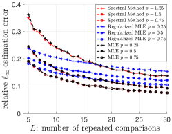
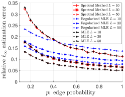
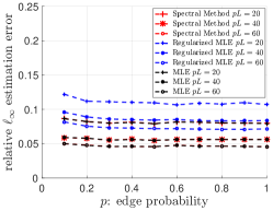
(a)	(b)	(c)

Figure 1: Empirical performance of the spectral method and the (regularized) MLE: (a) $\ell_{\infty}$ error vs. $L$, (b) $\ell_{\infty}$ error vs. $p$ and (c) $\ell_{\infty}$ error vs. $n^{2}pL$

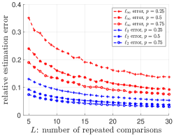
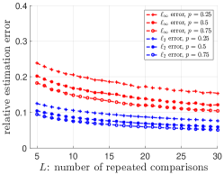
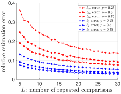
(a) spectral method	(b) regularized MLE	(c) MLE

Figure 2: Comparisons between the relative $\ell_{\infty}$ error and the relative $\ell_{2}$ error for (a) the spectral method, (b) the regularized MLE and (c) the MLE.

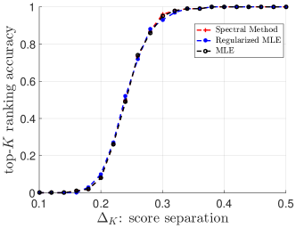
Figure 3: The top-$K$ ranking accuracy of both the spectral method and the regularized MLE.

We first investigate the $\ell_{\infty}$ error of the spectral method and the (regularized) MLE when estimating the preference scores. To this end, we generate the latent scores $w_{i}^{*}$ ($1\leq i\leq n$) independently and uniformly at random over the interval $\left[0.5,1\right]$. Figure 1(a) (resp. Figure 1(b)) displays the entrywise error in the spectral score estimation as the number of repeated comparisons $L$ (resp. the edge probability $p$) varies. As is seen from the plots, the $\ell_{\infty}$ error of all methods gets smaller as $p$ and $L$ increase, confirming our results in Theorems 3-4. Next, we show in Figure 1(c) the relative $\ell_{\infty}$ error while fixing the total number of samples (i.e. $n^{2}pL$). It can be seen that the performance almost does not change if the sample complexity $n^{2}pL$ remains the same. It is also interesting to see that the $\ell_{\infty}$ error of the spectral method and the MLE are very similar. In addition, Figure 2 illustrates the relative $\ell_{\infty}$ error and the relative $\ell_{2}$ error in score estimation for all three methods. As we can see, the relative $\ell_{\infty}$ errors are not much larger than the relative $\ell_{2}$ errors (recall that $n=200$), thus offering empirical evidence that the errors in the score estimates are spread out across all entries.

Further, we examine the top-$K$ ranking accuracy of all three methods. Here, we fix $p=0.25$ and $L=20$, set ${\it K}=10$, and let $w^{*}_{i}=1$ for all $1\leq i\leq K$ and $w^{*}_{j}=1-\Delta$ for all $K+1\leq j\leq n$. By construction, the score separation satisfies $\Delta_{K}=\Delta$. Figure 3 illustrates the accuracy in identifying the top-$K$ ranked items. The performance of them improves when the score separation becomes larger, which matches our theory in Theorem 1.

2.7 Other related works

The problem of ranking based on partial preferences has received much attention during the past decade. Two types of observation models have been considered: $(1)$ the cardinal-based model, where users provide explicit numerical ratings of the items, $(2)$ the ordinal-based model, where users are asked to make comparative measurements. See Ammar and Shah (2011) for detailed comparisons between them.

In terms of the ordinal-based model — and in particular, ranking from pairwise comparisons — both parametric and nonparametric models have been extensively studied. For example, Hunter (2004) examined variants of the parametric BTL model, and established the convergence properties of the minorization-maximization algorithm for computing the MLE. Moreover, the BTL model falls under the category of low-rank parametric models, since the preference matrix is generated by passing a rank-2 matrix through the logistic link function (Rajkumar and Agarwal, 2016). Additionally, the work Jiang et al. (2011) proposed a least-squares type method to estimate the full ranking, which generalizes the simple Borda count algorithm (Ammar and Shah, 2011). For many of these algorithms, the sample complexities needed for perfect total ranking were determined by Rajkumar and Agarwal (2014), although the top-$K$ ranking accuracy was not considered there.

Going beyond the parametric models, a recent line of works Shah et al. (2017); Shah and Wainwright (2015); Chen et al. (2017); Pananjady et al. (2017) considered the nonparametric stochastically transitive model, where the only model assumption is that the comparison probability matrix follows certain transitivity rules. This type of models subsumes the BTL model as a special case. For instance, Shah and Wainwright (2015) suggested a simple counting-based algorithm which can reliably recover the top-$K$ ranked items for various models. However, the sampling paradigm considered therein is quite different from ours in the sparse regime; for instance, their model does not come close to the setting where $p$ is small but $L$ is large, which is the most challenging regime of the model adopted in our paper and Negahban et al. (2017a); Chen and Suh (2015).

All of the aforementioned papers concentrate on the case where there is a single ground-truth ordering. It would also be interesting to investigate the scenarios where different users might have different preference scores. To this end, Negahban et al. (2017b); Lu and Negahban (2014) imposed the low-rank structure on the underlying preference matrix and adopted the nuclear-norm relaxation approach to recover the users’ preferences. Additionally, several papers explored the ranking problem for the more general Plackett-Luce model (Hajek et al., 2014; Soufiani et al., 2013), in the presence of adaptive sampling (Jamieson and Nowak, 2011; Busa-Fekete et al., 2013; Heckel et al., 2016; Agarwal et al., 2017), for the crowdsourcing scenario (Chen et al., 2013), and in the adversarial setting (Suh et al., 2017). These are beyond the scope of the present paper.

Speaking of the error metric, the $\ell_{\infty}$ norm is appropriate for top-$K$ ranking problem and other learning problems as well. In particular, $\ell_{\infty}$ perturbation bounds for eigenvectors of symmetric matrices (Koltchinskii and Lounici, 2016; Fan et al., 2016; Eldridge et al., 2017; Abbe et al., 2017) and singular vectors of general matrices (Koltchinskii and Xia, 2016) have been studied. In stark contrast, we study the $\ell_{\infty}$ norm errors of the leading eigenvector of a class of asymmetric matrices (probability transition matrix) and the regularized MLE. Furthermore, most existing results require the expectations of data matrices to have low rank, at least approximately. We do not impose such assumptions.

When it comes to the technical tools, it is worth noting that the leave-one-out idea has been invoked to analyze random designs for other high-dimensional problems, e.g. robust M-estimators (El Karoui, 2017), confidence intervals for Lasso (Javanmard and Montanari, 2015), likelihood ratio test (Sur et al., 2017), and nonconvex statistical learning (Ma et al., 2017; Chen et al., 2018). In particular, Zhong and Boumal (2017) and Abbe et al. (2017) use it to precisely characterize entrywise behavior of eigenvectors of a large class of symmetric random matrices, which improves upon prior $\ell_{\infty}$ eigenvector analysis. Consequently, they are able to show the sharpness of spectral methods in many popular models. Our introduction of leave-one-out auxiliary quantities is similar in spirit to these papers.

Finally, the family of spectral methods has been successfully applied in numerous applications, e.g. matrix completion (Keshavan et al., 2010), phase retrieval (Chen and Candès, 2017), graph clustering (Rohe et al., 2011; Abbe et al., 2017), joint alignment (Chen and Candes, 2016). All of them are designed based on the eigenvectors of some symmetric matrix, or the singular vectors if the matrix of interest is asymmetric. Our paper contributes to this growing literature by establishing a sharp eigenvector perturbation analysis framework for an important class of asymmetric matrices — the probability transition matrices.

3 Extension: general dynamic range

All of the preceding results concern the regime with a fixed dynamic range (i.e. $\kappa=O(1)$). This section moves on to discussing the case with large $\kappa$.

To start with, by going through the same proof technique, we can readily obtain — in the general $\kappa$ setting — the following performance guarantees for both the spectral estimate $\bm{\pi}$ and the regularized MLE $\bm{\theta}$.

Theorem 5.

Consider the pairwise comparison model in Section 2.1. Suppose that $p>\frac{c_{0}\kappa^{5}\log n}{n}$ for some sufficiently large constant $c_{0}>0$, and choose $d=c_{d}np$ for some constant $c_{d}\geq 2$ in Algorithm 1. Then with probability exceeding $1-O\big{(}n^{-5}\big{)}$,

1. the spectral estimate $\bm{\pi}$ satisfies

   $$\frac{\left\|\bm{\pi}-\bm{\pi}^{*}\right\|_{\infty}}{\left\|\bm{\pi}^{*}\right\|_{\infty}}\lesssim\kappa\sqrt{\frac{\log n}{npL}},$$

   where $\bm{\pi}^{*}$ is the normalized score vector as defined in (10).

2. the set of top-$K$ ranked items can be recovered exactly by the spectral method given in Algorithm 1, as long as

   $$\frac{n^{2}pL}{2}\geq c_{1}\frac{\kappa^{2}n\log n}{\Delta_{K}^{2}}$$

   for some sufficiently large constant $c_{1}>0$.

Theorem 6.

Consider the pairwise comparison model in Section 2.1. Suppose that $p\geq\frac{c_{0}\kappa^{4}\log n}{n}$ for some sufficiently large constant $c_{0}>0$ and that $L\leq c_{2}\cdot n^{c_{3}}$ for any absolute constants $c_{2},c_{3}>0$. Set the regularization parameter to be $\lambda=c_{\lambda}\frac{1}{\log\kappa}\sqrt{\frac{np\log n}{L}}$ for some absolute constant $c_{\lambda}>0$. Then with probability exceeding $1-O\big{(}n^{-5}\big{)}$,

1. the regularized MLE $\bm{\theta}$ satisfies

   $$\frac{\big{\|}e^{\bm{\theta}}-e^{\bm{\theta}^{*}-\overline{\theta}^{*}\bm{1}}\big{\|}_{\infty}}{\big{\|}e^{\bm{\theta}^{*}-\overline{\theta}^{*}\bm{1}}\big{\|}_{\infty}}\lesssim\kappa^{2}\sqrt{\frac{\log n}{npL}}$$

   where $\overline{\theta}^{*}:=\frac{1}{n}\bm{1}^{\top}\bm{\theta}^{*}$ and $e^{\bm{\theta}}:=[e^{\theta_{1}},\cdots,e^{\theta_{n}}]^{\top}$.

2. the set of top-$K$ ranked items can be recovered exactly by the regularized MLE given in (13), as long as

   $$\frac{n^{2}pL}{2}\geq c_{1}\frac{\kappa^{4}n\log n}{\Delta_{K}^{2}}$$

   for some sufficiently large constant $c_{1}>0$.

Remark 4.

The guarantees on exact top-$K$ recovery for both the spectral method and the regularized MLE are immediate consequences of their $\ell_{\infty}$ error bound, as we have argued in Section 2.4. Hence we will focus on proving the $\ell_{\infty}$ error bound in Sections 5–6.

Notably, the achievability bounds for top-$K$ ranking in Theorems 5–6 do not match the lower bound asserted in Theorem 2 in terms of $\kappa$. This is partly because the separation measure $\Delta_{K}$ fails to capture the information bottleneck for the general $\kappa$ setting. In light of this, we introduce the following new measure that seems to be a more suitable metric to reflect the hardness of the top-$K$ ranking problem:

$$\Delta_{K}^{*}:=\frac{w_{K}^{*}-w_{K+1}^{*}}{w_{K+1}^{*}}\cdot\sqrt{\frac{1}{n}\sum\nolimits_{i=1}^{n}\frac{w_{K+1}^{*}w_{i}^{*}}{\left(w_{K}^{*}+w_{i}^{*}\right)^{2}}},$$ (33)

which will be termed the generalized separation measure. Informally, $(\Delta_{K}^{*})^{2}$ is a reasonably tight upper bound on certain normalized KL divergence metric. With this metric in place, we derive another lower bound as follows.

Theorem 7.

Fix $\epsilon\in(0,\frac{1}{2})$, and let $\mathcal{G}\sim\mathcal{G}_{n,p}$. Consider any preference score vector $\bm{w}^{*}$, and let $\Delta_{K}^{*}$ denote its generalized separation. If

$$n^{2}pL\leq\frac{\epsilon^{2}}{2}\frac{n}{(\Delta_{K}^{*})^{2}},$$

then there exists another preference score vector $\tilde{\bm{w}}$ with the same generalized separation $\Delta_{K}^{*}$ and different top-$K$ items such that $P_{\mathrm{e}}(\psi)\geq\frac{1-\epsilon}{2}$ for any ranking scheme $\psi$. Here, $P_{\mathrm{e}}(\psi)$ represents the probability of error in distinguishing these two vectors given $\bm{y}$.

Proof.

See Appendix A.∎

The preceding sample complexity lower bound scales inversely proportionally to $\left(\Delta_{K}^{*}\right)^{2}$. To see why this generalized measure may be more suitable compared to the original separation metric, we single out three examples in Appendix B. Unfortunately, our current analyses do not yield a matching upper bound with respect to $\Delta_{K}^{*}$ unless $\kappa$ is a constant. For instance, the analysis of the spectral method relies on the eigenvector perturbation bound (Theorem 8), where the spectral gap and matrix perturbation play a crucial rule. However, the current results for controlling these quantities have explicit dependency on $\kappa$ Negahban et al. (2017a). It is not clear whether we could incorporate the new measure to eliminate such dependency on $\kappa$. This calls for more refined analysis techniques, which we leave for future investigation.

Moreover, it is not obvious whether the spectral method alone or the regularized MLE alone can achieve the minimal sample complexity in the general $\kappa$ regime. It is possible that one needs to first screen out those items with extremely high or low scores using methods like Borda count (Ammar and Shah, 2012), as advocated by (Negahban et al., 2017a; Chen and Suh, 2015; Jang et al., 2016). All in all, finding tight upper bounds for general $\kappa$ remains an open question.

4 Discussion

This paper justifies the optimality of both the spectral method and the regularized MLE for top-$K$ rank aggregation for the fixed dynamic range case. Our theoretical studies are by no means exhaustive, and there are numerous directions that would be of interest for future investigations. We point out a few possibilities as follows.

General condition number $\kappa$. As mentioned before, our current theory is optimal in the presence of a fixed dynamic range with $\kappa=O\left(1\right)$. We have also made a first attempt in considering the large $\kappa$ regime. It is desirable to characterize the statistical and computational limits for more general $\kappa$.

Goodness-of-fit. Throughout this paper, we have assumed the BTL model captures the randomness underlying the data we collect. A practical question is whether the real data actually follows the BTL model. It would be interesting to investigate how to test the goodness-of-fit of this model.

Unregularized MLE. We have studied the optimality of the regularized MLE with the regularization parameter $\lambda\asymp\sqrt{\frac{np\log n}{L}}$. Our analysis relies on the regularization term to obtain convergence of the gradient descent algorithm (see Lemma 11). It is natural to ask whether such a regularization term is necessary or not. This question remains open.

More general comparison graphs. So far we have focused on a tractable but somewhat restrictive comparison graph, namely, the Erdős–Rényi random graph. It would certainly be important to understand the performance of both methods under a broader family of comparison graphs, and to see which algorithms would enable optimal sample complexities under general sampling patterns.

Entrywise perturbation analysis for convex optimization. This paper provides the $\ell_{\infty}$ perturbation analysis for the regularized MLE using the leave-one-out trick as well as an inductive argument along the algorithmic updates. We expect this analysis framework to carry over to a much broader family of convex optimization problems, which may in turn offer a powerful tool for showing the stability of optimization procedures in an entrywise fashion.

5 Analysis for the spectral method

This section is devoted to proving Theorem 5 and hence Theorem 3, which characterizes the pointwise error of the spectral estimate.

5.1 Preliminaries

Here, we gather some preliminary facts about reversible Markov chains as well as the Erdős–Rényi random graph.

The first important result concerns the eigenvector perturbation for probability transition matrices, which can be treated as the analogue of the celebrated Davis-Kahan $\sin\Theta$ theorem (Davis and Kahan, 1970). Due to its potential importance for other problems, we promote it to a theorem as follows.

Theorem 8 (Eigenvector perturbation).

Suppose that $\bm{P}$, $\hat{\bm{P}}$, and $\bm{P}^{*}$ are probability transition matrices with stationary distributions $\bm{\pi}$, $\hat{\bm{\pi}}$, $\bm{\pi}^{*}$, respectively. Also, assume that $\bm{P}^{*}$ represents a reversible Markov chain. When $\big{\|}\bm{P}-\hat{\bm{P}}\big{\|}_{\bm{\pi}^{*}}<1-\max\left\{\lambda_{2}(\bm{P}^{*}),-\lambda_{n}\left(\bm{P}^{*}\right)\right\}$, it holds that

$$\|\bm{\pi}-\hat{\bm{\pi}}\|_{\bm{\pi}^{*}}\leq\frac{\big{\|}\bm{\pi}^{\top}(\bm{P}-\hat{\bm{P}})\big{\|}_{\bm{\pi}^{*}}}{1-\max\left\{\lambda_{2}(\bm{P}^{*}),-\lambda_{n}\left(\bm{P}^{*}\right)\right\}-\big{\|}\bm{P}-\hat{\bm{P}}\big{\|}_{\bm{\pi}^{*}}}.$$

Proof.

See Appendix C.1. ∎

Several remarks regarding Theorem 8 are in order. First, in contrast to standard perturbation results like Davis-Kahan’s $\sin\Theta$ theorem, our theorem involves three matrices in total, where $\bm{P}$, $\hat{\bm{P}}$, and $\bm{P}^{*}$ can all be arbitrary. For example, one may choose $\bm{P}^{*}$ to be the population transition matrix, and $\bm{P}$ and $\hat{\bm{P}}$ as two finite-sample versions associated with $\bm{P}^{*}$. Second, we only impose reversibility on $\bm{P}^{*}$, whereas $\bm{P}$ and $\hat{\bm{P}}$ need not induce reversible Markov Chains. Third, Theorem 8 allows one to derive the $\ell_{2}$ estimation error in Negahban et al. (2017a) directly without resorting to the power method; in fact, our $\ell_{2}$ estimation error bound improves upon Negahban et al. (2017a) by some logarithmic factor.

Theorem 9.

Consider the pairwise comparison model specified in Section 2.1 with $\kappa=O(1)$. Suppose $p\geq c_{0}\frac{\log n}{n}$ for some sufficiently large constant $c_{0}>0$ and $d\geq c_{d}np$ for $c_{d}\geq 2$ in Algorithm 1. With probability exceeding $1-O(n^{-5})$, one has

$$\frac{\|\bm{\pi}-\bm{\pi}^{*}\|_{2}}{\|\bm{\pi^{*}}\|_{2}}\lesssim\frac{1}{\sqrt{npL}}.$$

Proof.

See Appendix C.2. ∎

Notably, Theorem 9 matches the minimax lower bound derived in (Negahban et al., 2017a, Theorem 3). As far as we know, this is the first result that demonstrates the orderwise optimality of the spectral method when measured by the $\ell_{2}$ loss.

The next result is concerned with the concentration of the vertex degrees in an Erdős–Rényi random graph.

Lemma 1 (Degree concentration).

Suppose that $\mathcal{G}\sim\mathcal{G}_{n,p}$. Let $d_{i}$ be the degree of node $i$, $d_{\min}=\min_{1\leq i\leq n}d_{i}$ and $d_{\max}=\max_{1\leq i\leq n}d_{i}$. If $p\geq\frac{c_{0}\log n}{n}$ for some sufficiently large constant $c_{0}>0$, then the following event

$$\mathcal{A}_{0}=\left\{\frac{np}{2}\leq d_{\min}\leq d_{\max}\leq\frac{3np}{2}\right\}$$ (34)

obeys

$$\mathbb{P}\left(\mathcal{A}_{0}\right)\geq 1-O(n^{-10}).$$

Proof.

The proof follows from the standard Chernoff bound and is hence omitted. ∎

Since $d$ is chosen to be $c_{d}np$ for some constant $c_{d}\geq 2$, we have, by Lemma 1, that the maximum vertex degree obeys $d_{\max}<d$ with high probability.

5.2 Proof outline of Theorem 5

In this subsection, we outline the proof of Theorem 5.

Recall that $\bm{\pi}=\left[\pi_{1},\cdots,\pi_{n}\right]^{\top}$ and $\bm{\pi}^{*}=\left[\pi_{1}^{*},\cdots,\pi_{n}^{*}\right]^{\top}$ are the stationary distributions associated with $\bm{P}$ and $\bm{P}^{*}$, respectively. This gives

$$\bm{\pi}^{\top}\bm{P}=\bm{\pi}^{\top}\qquad\text{and}\qquad\bm{\pi}^{*\top}\bm{P}^{*}=\bm{\pi}^{*\top}.$$

For each $1\leq m\leq n$, one can decompose

$$\pi_{m}-\pi_{m}^{*} =\bm{\pi}^{\top}\bm{P}_{\cdot m}-\bm{\pi}^{*\top}\bm{P}_{\cdot m}^{*}=\bm{\pi}^{*\top}\left(\bm{P}_{\cdot m}-\bm{P}_{\cdot m}^{*}\right)+\left(\bm{\pi}-\bm{\pi}^{*}\right)^{\top}\bm{P}_{\cdot m}$$

$$=\underset{:=I_{1}^{m}}{\underbrace{\sum_{j}\pi_{j}^{*}\left(P_{j,m}-P_{j,m}^{*}\right)}}+\underset{:=I_{2}^{m}}{\underbrace{\left(\pi_{m}-\pi_{m}^{*}\right)P_{m,m}\vphantom{\sum_{j}\pi_{j}^{*}}}}+\sum_{j:j\neq m}\left(\pi_{j}-\pi_{j}^{*}\right)P_{j,m},$$

where $\bm{P}_{\cdot m}$ (resp. $\bm{P}^{*}_{\cdot m}$) denotes the $m$-th column of $\bm{P}$ (resp. $\bm{P}^{*}$). Then it boils down to controlling $I_{1}^{m}$, $I_{2}^{m}$ and $\sum_{j:j\neq m}(\pi_{j}-\pi_{j}^{*})P_{j,m}$.

1. Since $\bm{\pi}^{*}$ is deterministic while $\bm{P}$ is random, we can easily control $I_{1}^{m}$ using Hoeffding’s inequality. The bound is the following.

   Lemma 2.

   With probability exceeding $1-O(n^{-5})$, one has

   $$\max_{m}|I_{1}^{m}|\lesssim\sqrt{\frac{\log n}{Ld}}\|\bm{\pi}^{*}\|_{\infty}.$$

   Proof.

   See Appendix C.3. ∎

2. Next, we show the term $I_{2}^{m}$ behaves as a contraction of $|\pi_{m}-\pi_{m}^{*}|$.

   Lemma 3.

   With probability exceeding $1-O(n^{-5})$, there exists some constant $c>0$ such that for all $1\leq m\leq n$,

   $$|I_{2}^{m}|\leq\left(1-\frac{np}{2(1+\kappa)d}+c\sqrt{\frac{\log n}{Ld}}\right)|\pi_{m}-\pi_{m}^{*}|.$$

   Proof.

   See Appendix C.4. ∎

3. The statistical dependency between $\bm{\pi}$ and $\bm{P}$ introduces difficulty in obtaining a sharp estimate of the third term $\sum_{j:j\neq m}(\pi_{j}-\pi_{j}^{*})P_{j,m}$. Nevertheless, the leave-one-out technique helps us decouple the dependency and obtain effective control of this term. The key component of the analysis is the introduction of a new probability transition matrix $\bm{P}^{(m)}$, which is a leave-one-out version of the original matrix $\bm{P}$. More precisely, $\bm{P}^{(m)}$ replaces all of the transition probabilities involving the $m$-th item with their expected values (unconditional on $\mathcal{G}$); that is, for any $i\neq j$,

   $$P_{i,j}^{(m)}:=\begin{cases}P_{i,j},&\quad i\neq m,\text{ }j\neq m\\ \frac{p}{d}y_{i,j}^{*},&\quad i=m\text{ or }j=m\end{cases}$$

   with $y_{i,j}^{*}:=\frac{w_{j}^{*}}{w_{i}^{*}+w_{j}^{*}}$. For any $1\leq i\leq n$, set

   $$P_{i,i}^{(m)}:=1-\sum\nolimits_{j:j\neq i}P_{i,j}^{(m)}$$

   in order to ensure that $\bm{P}^{(m)}$ is a probability transition matrix. In addition, we let $\bm{\pi}^{\left(m\right)}$ be the stationary distribution of the Markov chain induced by $\bm{P}^{(m)}$. As will be demonstrated later, the main advantages of introducing $\bm{\pi}^{(m)}$ are two-fold: (1) the original spectral estimate $\bm{\pi}$ is very well approximated by $\bm{\pi}^{(m)}$, and (2) $\bm{\pi}^{(m)}$ is statistically independent of the connectivity of the $m$-th node and the comparisons with regards to the $m$-th item. Now we further decompose $\sum_{j:j\neq m}(\pi_{j}-\pi_{j}^{*})P_{j,m}$:

   $$\sum\nolimits_{j:j\neq m}\left(\pi_{j}-\pi_{j}^{*}\right)P_{j,m}=\underbrace{\sum\nolimits_{j:j\neq m}(\pi_{j}-\pi_{j}^{(m)})P_{j,m}}_{:=I_{3}^{m}}+\underbrace{\sum\nolimits_{j:j\neq m}(\pi_{j}^{(m)}-\pi_{j}^{*})P_{j,m}}_{:=I_{4}^{m}}.$$

4. For $I_{3}^{m}$, we apply the Cauchy-Schwarz inequality to obtain that with probability at least $1-O(n^{-10}),$

   $$|I_{3}^{m}|\leq\|\bm{\pi}^{(m)}-\bm{\pi}\|_{2}\left(\sum\nolimits_{j:j\neq m}P_{j,m}^{2}\right)^{\frac{1}{2}}\overset{\left(\text{i}\right)}{\leq}\frac{1}{\sqrt{d}}\|\bm{\pi}^{(m)}-\bm{\pi}\|_{2},$$

   where $\left(\text{i}\right)$ follows from the fact that $P_{j,m}\leq\frac{1}{d}$ for all $j\neq m$ and $d_{\max}\leq d$ on the event $\mathcal{A}_{0}$ (defined in Lemma 1). Consequently, it suffices to control the $\ell_{2}$ difference between the original spectral estimate $\bm{\pi}$ and its leave-one-out version $\bm{\pi}^{\left(m\right)}$. This is accomplished in the following lemma.

   Lemma 4.

   Suppose that $np\gamma^{2}>c\kappa\log n$ for some sufficiently large constant $c>0$. With probability at least $1-O\left(n^{-5}\right)$,

   $$\|\bm{\pi}^{(m)}-\bm{\pi}\|_{2} \leq\frac{16\sqrt{\kappa}}{\gamma}\sqrt{\frac{\log n}{Ld}}\|\bm{\pi}^{*}\|_{\infty}+\|\bm{\pi}-\bm{\pi}^{*}\|_{\infty},$$ (35)

   where $\kappa=w_{\max}/w_{\min}$ and $\gamma=1-\max\left\{\lambda_{2}(\bm{P}^{*}),-\lambda_{n}\left(\bm{P}^{*}\right)\right\}-\|\bm{P}-\bm{P}^{*}\|_{\bm{\pi}^{*}}$.

   Proof.

   See Appendix C.5. ∎

   Using (Negahban et al., 2017a, Lemmas 3 and 4) and our Lemma 1, we can bound $\gamma$ from below:

   Lemma 5 (Spectral gap, Negahban et al. (2017a)).

   Under the model specified in Section 2.1, if $p\geq c_{0}\frac{\log n}{n}\max\{1,\frac{\kappa^{5}}{L}\}$ for some sufficiently large constant $c_{0}>0$, then with probability at least $1-O(n^{-5})$,

   $$\gamma:=1-\max\left\{\lambda_{2}(\bm{P}^{*}),-\lambda_{n}\left(\bm{P}^{*}\right)\right\}-\|\bm{P}-\bm{P}^{*}\|_{\bm{\pi}^{*}}\geq\frac{1}{2\kappa^{2}}\frac{d_{\min}}{d_{\max}}\geq\frac{1}{6\kappa^{2}}.$$

5. In order to control $I_{4}^{m}$, we exploit the statistical independence between $\bm{\pi}^{(m)}$ and $\bm{P}_{\cdot m}$. Specifically, we demonstrate that:

   Lemma 6.

   Suppose that $p>\frac{c_{0}\log n}{n}$ for some sufficiently large constant $c_{0}>0$. With probability at least $1-O\left(n^{-10}\right)$,

   $$|I_{4}^{m}|\lesssim\frac{1}{\sqrt{n}}\|\bm{\pi}^{(m)}-\bm{\pi}\|_{2}+\sqrt{\frac{\log n}{Ld}}\|\bm{\pi}^{*}\|_{\infty}+\frac{\sqrt{np\log n}+\log n}{d}\|\bm{\pi}^{(m)}-\bm{\pi}^{*}\|_{\infty}.$$

   Proof.

   See Appendix C.6. ∎

   The above bound depends on both $\|\bm{\pi}^{(m)}-\bm{\pi}\|_{2}$ and $\|\bm{\pi}^{(m)}-\bm{\pi}^{*}\|_{\infty}$. We can invoke Lemma 4 and the inequality $\|\bm{\pi}^{(m)}-\bm{\pi}^{*}\|_{\infty}\leq\|\bm{\pi}^{(m)}-\bm{\pi}\|_{2}+\|\bm{\pi}-\bm{\pi}^{*}\|_{\infty}$ to reach

   $$|I_{4}^{m}| \lesssim\left(\frac{1}{\sqrt{n}}+\frac{\sqrt{np\log n}+\log n}{d}\right)\|\bm{\pi}^{(m)}-\bm{\pi}\|_{2}+\sqrt{\frac{\log n}{Ld}}\|\bm{\pi}^{*}\|_{\infty}$$

   $$\quad+\frac{\sqrt{np\log n}+\log n}{d}\|\bm{\pi}-\bm{\pi}^{*}\|_{\infty}$$

   $$\lesssim\left\{\left(\frac{1}{\sqrt{n}}+\frac{\sqrt{np\log n}+\log n}{d}\right)\frac{\sqrt{\kappa}}{\gamma}+1\right\}\sqrt{\frac{\log n}{Ld}}\|\bm{\pi}^{*}\|_{\infty}$$

   $$\quad+\left(\frac{1}{\sqrt{n}}+\frac{\sqrt{np\log n}+\log n}{d}\right)\|\bm{\pi}-\bm{\pi}^{*}\|_{\infty}.$$

6. Finally we put the preceding bounds together. When $\frac{np}{\kappa^{5}\log n}$ is large enough, with high probability, for some absolute constants $c_{1},c_{2},c_{3}>0$ one has

   $$\left(\frac{np}{2(1+\kappa)d}-c_{1}\sqrt{\frac{\log n}{Ld}}\right)|\pi_{m}-\pi_{m}^{*}|$$

   $$\quad\leq\left\{c_{2}+\left(\frac{1}{\sqrt{d}}+\frac{c_{3}}{\sqrt{n}}+c_{3}\frac{\sqrt{np\log n}+\log n}{d}\right)\frac{16\sqrt{\kappa}}{\gamma}\right\}\sqrt{\frac{\log n}{Ld}}\|\bm{\pi}^{*}\|_{\infty}$$

   $$\quad+\left(\frac{1}{\sqrt{d}}+\frac{c_{3}}{\sqrt{n}}+2c_{3}\frac{\sqrt{np\log n}+\log n}{d}\right)\|\bm{\pi}-\bm{\pi}^{*}\|_{\infty}.$$

   simultaneously for all $1\leq m\leq n$. By taking the maximum over $m$ on the left-hand side and combining terms, we get

   $$\underset{:=\alpha_{1}}{\underbrace{\left(\frac{np}{2(1+\kappa)d}-c_{1}\sqrt{\frac{\log n}{Ld}}-\frac{1}{\sqrt{d}}-\frac{c_{3}}{\sqrt{n}}-2c_{3}\frac{\sqrt{np\log n}+\log n}{d}\right)}}\|\bm{\pi}-\bm{\pi}^{*}\|_{\infty}$$

   $$\qquad\leq\underset{:=\alpha_{2}}{\underbrace{\left\{c_{2}+\left(\frac{1}{\sqrt{d}}+\frac{c_{3}}{\sqrt{n}}+c_{3}\frac{\sqrt{np\log n}+\log n}{d}\right)\frac{16\sqrt{\kappa}}{\gamma}\right\}}}\sqrt{\frac{\log n}{Ld}}\|\bm{\pi}^{*}\|_{\infty}.$$

   Hence, as long as $\frac{np}{\kappa^{5}\log n}$ is sufficiently large, one has

   $$c_{1}\sqrt{\frac{\log n}{Ld}}+\frac{1}{\sqrt{d}}+\frac{c_{3}}{\sqrt{n}}+2c_{3}\frac{\sqrt{np\log n}+\log n}{d}\lesssim\sqrt{\frac{\log n}{np}}\lesssim\frac{1}{\sqrt{\kappa^{5}}},$$

   which further leads to $\alpha_{1}\gtrsim 1/\kappa$, $\alpha_{2}\lesssim 1$, and

   $$\|\bm{\pi}-\bm{\pi}^{*}\|_{\infty}\lesssim\kappa\sqrt{\frac{\log n}{Ld}}\|\bm{\pi}^{*}\|_{\infty}\asymp\kappa\sqrt{\frac{\log n}{npL}}\|\bm{\pi}^{*}\|_{\infty}.$$

   This finishes the proof of Theorem 5 and Theorem 3.

6 Analysis for the regularized MLE

This section establishes the $\ell_{\infty}$ error of the regularized MLE as claimed in Theorem 6 (and also Theorem 4). Recall that in Theorem 6, we compare the regularized MLE $\bm{\theta}$ with $\bm{\theta}^{*}-\overline{\theta}^{*}\bm{1}$. Therefore, without loss of generality we can assume that

$$\bm{1}^{\top}\bm{\theta}^{*}=0.$$ (36)

This combined with the fact that $\theta_{\max}-\theta_{\min}=\log\kappa$ reveals that

$$\left\|\bm{\theta}^{*}\right\|_{\infty}\leq\log\kappa\qquad\text{and}\qquad\left\|\bm{\theta}^{*}\right\|_{2}\leq\sqrt{n}\log\kappa.$$

In addition, we assume that $L=O\left(n^{5}\right)$ in this section. It is straightforward to extend the proof to cover $L\leq c_{2}\cdot n^{c_{3}}$ for any constants $c_{2},c_{3}>0$.

6.1 Preliminaries and notation

Before proceeding to the proof, we gather some basic facts. To begin with, the gradient and the Hessian of $\mathcal{L}\left(\cdot;\bm{y}\right)$ in (12) can be computed as

$$\nabla\mathcal{L}\left(\bm{\theta};\bm{y}\right) =\sum_{(i,j)\in\mathcal{E},i>j}\left\{-y_{j,i}+\frac{e^{\theta_{i}}}{e^{\theta_{i}}+e^{\theta_{j}}}\right\}\left(\bm{e}_{i}-\bm{e}_{j}\right);$$ (37)

$$\nabla^{2}\mathcal{L}\left(\bm{\theta};\bm{y}\right) =\sum_{(i,j)\in\mathcal{E},i>j}\frac{e^{\theta_{i}}e^{\theta_{j}}}{\left(e^{\theta_{i}}+e^{\theta_{j}}\right)^{2}}\left(\bm{e}_{i}-\bm{e}_{j}\right)\left(\bm{e}_{i}-\bm{e}_{j}\right)^{\top}.$$ (38)

Here $\bm{e}_{1},\cdots,\bm{e}_{n}$ stand for the canonical basis vectors in $\mathbb{R}^{n}$. When evaluated at the truth $\bm{\theta}^{*}$, the size of the gradient can be controlled as follows.

Lemma 7.

Let $\lambda$ be as specified in Theorem 6. The following event

$$\mathcal{A}_{2}:=\left\{\left\|\nabla\mathcal{L}_{\lambda}\left(\bm{\theta}^{*};\bm{y}\right)\right\|_{2}\lesssim\sqrt{\frac{n^{2}p\log n}{L}}\right\}.$$ (39)

occurs with probability exceeding $1-O(n^{-10})$.

Proof.

See Appendix D.1.∎

The following lemmas characterize the smoothness and the strong convexity of the function $\mathcal{L}_{\lambda}\left(\cdot;\bm{y}\right)$. In the sequel, we denote by $\bm{L}_{\mathcal{G}}=\sum_{(i,j)\in\mathcal{E},i>j}\left(\bm{e}_{i}-\bm{e}_{j}\right)\left(\bm{e}_{i}-\bm{e}_{j}\right)^{\top}$ the (unnormalized) Laplacian matrix (Chung, 1997) associated with $\mathcal{G}$. For any matrix $\bm{A}$ we let

$$\lambda_{\min,\perp}(\bm{A}):=\min\left\{\mu\mid\bm{z}^{\top}\bm{A}\bm{z}\geq\mu\|\bm{z}\|_{2}^{2}\text{ for all }\bm{z}\text{ with }\bm{1}^{\top}\bm{z}=0\right\},$$ (40)

namely, the smallest eigenvalue when restricted to vectors orthogonal to $\bm{1}$.

Lemma 8.

Suppose that $p>\frac{c_{0}\log n}{n}$ for some sufficiently large constant $c_{0}>0$. Then on the event $\mathcal{A}_{0}$ as defined in (34), one has

$$\lambda_{\max}\left(\nabla^{2}\mathcal{L}_{\lambda}\left(\bm{\theta};\bm{y}\right)\right)\leq\lambda+np,\qquad\forall\bm{\theta}\in\mathbb{R}^{n}.$$

Proof.

Note that $\frac{e^{\theta_{i}}e^{\theta_{j}}}{(e^{\theta_{i}}+e^{\theta_{j}})^{2}}\leq\frac{1}{4}$. It follows immediately from the Hessian in (38) that

$$\lambda_{\max}\left(\nabla^{2}\mathcal{L}_{\lambda}\left(\bm{\theta};\bm{y}\right)\right)\leq\lambda+\frac{1}{4}\left\|\bm{L}_{\mathcal{G}}\right\|\leq\lambda+\frac{1}{2}d_{\max},$$

where $d_{\max}$ is the maximum vertex degree in the graph $\mathcal{G}$. In addition, on the event $\mathcal{A}_{0}$ we have $d_{\max}\leq 2np$, which completes the proof. ∎

Lemma 9.

For all $\bm{\theta}\in\mathbb{R}^{n}$ such that $\left\|\bm{\theta}-\bm{\theta}^{*}\right\|_{\infty}\leq C$ for some $C\geq 0$, we have

$$\lambda_{\min,\perp}\left(\nabla^{2}\mathcal{L}_{\lambda}\left(\bm{\theta};\bm{y}\right)\right)\geq\lambda+\frac{1}{4\kappa e^{2C}}\lambda_{\min,\perp}\left(\bm{L}_{\mathcal{G}}\right).$$

Proof.

See Appendix D.2.∎

Lemma 10.

Let $\mathcal{G}\sim\mathcal{G}_{n,p}$, and suppose that $p>\frac{c_{0}\log n}{n}$ for some sufficiently large constant $c_{0}>0$. Then one has

$$\mathbb{P}\left(\lambda_{\min,\perp}\left(\bm{L}_{\mathcal{G}}\right)\geq np/2\right)\geq 1-O\left(n^{-10}\right).$$

Proof.

Note that $\lambda_{\min,\perp}\left(\bm{L}_{\mathcal{G}}\right)$ is exactly the spectral gap of the Laplacian matrix. See (Tropp, 2015, Sec 5.3.3) for the derivation of this lemma. ∎

By combining Lemma 9 with Lemma 10, we reach the following result.

Corollary 1.

Under the assumptions of Lemma 10, with probability exceeding $1-O\left(n^{-10}\right)$ one has

$$\lambda_{\min,\perp}\left(\nabla^{2}\mathcal{L}_{\lambda}\left(\bm{\theta};\bm{y}\right)\right)\geq\lambda+\frac{1}{8\kappa e^{2C}}np$$

simultaneously for all $\bm{\theta}$ obeying $\left\|\bm{\theta}-\bm{\theta}^{*}\right\|_{\infty}\leq C$ for some $C\geq 0$.

6.2 Proof outline of Theorem 6

This subsection outlines the main steps for establishing Theorem 6.

Rather than directly resorting to the optimality condition, we adopt an algorithmic perspective to analyze the regularized MLE $\bm{\theta}$. Specifically, we consider the standard gradient descent algorithm that is expected to converge to the minimizer $\bm{\theta}$, and analyze the trajectory of this iterative algorithm instead. The algorithm is stated in Algorithm 2.

  Initialize $\bm{\theta}^{0}=\bm{\theta}^{*}$.

  for $t=0,1,2,\ldots,T-1$ do

     

$$\bm{\theta}^{t+1}=\bm{\theta}^{t}-\eta_{t}\nabla\mathcal{L}_{\lambda}\left(\bm{\theta}^{t};\bm{y}\right);$$ (41)

  end for

Algorithm 2 Gradient descent for computing the regularized MLE.

Notably, this gradient descent algorithm is not practical since the initial point is set to be $\bm{\theta}^{*}$. Nevertheless, it is helpful for analyzing the statistical accuracy of the regularized MLE $\bm{\theta}$. In what follows, we shall adopt a time-invariant step size rule:

$$\eta_{t}\equiv\eta=\frac{1}{\lambda+np},\qquad t=0,1,2,\cdots$$ (42)

Our proof can be divided into three steps:

1. establish — via standard optimization theory — that the output $\bm{\theta}^{T}$ of Algorithm 2 is sufficiently close to the regularized MLE $\bm{\theta}$, namely,

   $$\left\|\bm{\theta}^{T}-\bm{\theta}\right\|_{\infty}\leq\left\|\bm{\theta}^{T}-\bm{\theta}\right\|_{2}\leq C_{0}\kappa^{2}\sqrt{\frac{\log n}{npL}}$$ (43)

   for $T=n^{5}$, where $C_{0}>0$ is some absolute constant;

2. use the leave-one-out argument to demonstrate that: the output $\bm{\theta}^{T}$ is close to the truth $\bm{\theta}^{*}$ in an entrywise fashion, i.e.

   $$\left\|\bm{\theta}^{T}-\bm{\theta}^{*}\right\|_{\infty}\leq C_{4}\kappa^{2}\sqrt{\frac{\log n}{npL}}$$

   for some universal constant $C_{4}>0$. Combining this with (43) yields

   $$\left\|\bm{\theta}-\bm{\theta}^{*}\right\|_{\infty}\lesssim\kappa^{2}\sqrt{\frac{\log n}{npL}};$$

3. the final step is to translate the perturbation bound on $\|\bm{\theta}-\bm{\theta}^{*}\|_{\infty}$ to $\|e^{\bm{\theta}}-e^{\bm{\theta}^{*}}\|_{\infty}$ as claimed in the theorem.

Before continuing, we single out an important fact that will be used throughout the proof.

Fact 1.

Suppose $\bm{1}^{\top}\bm{\theta}^{*}=0$. Then we have $\bm{1}^{\top}\bm{\theta}^{t}=0$ for all $t\geq 0$.

Proof.

See Appendix D.3. ∎

6.3 Step I

The first step relies heavily on optimization theory, namely the theory of gradient descent on strongly convex and smooth functions.

1. It is seen that the sequence $\left\{\bm{\theta}^{t}\right\}_{t=1}^{\infty}$ converges geometrically fast to the regularized MLE $\bm{\theta}$, a property that is standard in convex optimization literature. This claim is summarized in the following lemma.

   Lemma 11.

   On the event $\mathcal{A}_{0}$ as defined in (34), one has

   $$\left\|\bm{\theta}^{t}-\bm{\theta}\right\|_{2}\leq\rho^{t}\left\|\bm{\theta}^{0}-\bm{\theta}\right\|_{2},$$

   where $\rho=1-\frac{\lambda}{\lambda+np}$.

   Proof.

   This result directly follows from the smoothness property (see Lemma 8), the trivial strong convexity of $\mathcal{L}_{\lambda}\left(\bm{\theta};\bm{y}\right)$ ($\nabla^{2}\mathcal{L}_{\lambda}\left(\bm{\theta};\bm{y}\right)\succeq\lambda\bm{I}_{n},\;\forall\bm{\theta}$), as well as the convergence property of the gradient descent algorithm (e.g. (Bubeck, 2015, Theorem 3.10)). ∎

   A direct consequence of this convergence result and Fact 1 is that $\bm{1}^{\top}\bm{\theta}=0$ for the regularized MLE $\bm{\bm{\theta}}$.

2. We then control $\|\bm{\theta}^{0}-\bm{\theta}\|_{2}$. Recall that $\bm{\theta}^{0}=\bm{\theta}^{*}$, and we have:

   Lemma 12.

   On the event $\mathcal{A}_{2}$ as defined in (39), there exists some constant $c_{2}>0$ such that

   $$\|\bm{\theta}^{0}-\bm{\theta}\|_{2}=\left\|\bm{\theta}-\bm{\theta}^{*}\right\|_{2}\leq c_{2}\sqrt{n}\log\kappa.$$

   Proof.

   See Appendix D.4. ∎

3. The previous two claims taken together lead us to conclude that

   $$\left\|\bm{\theta}^{T}-\bm{\theta}\right\|_{2} \leq\rho^{T}\|\bm{\theta}^{0}-\bm{\theta}\|_{2}\leq\rho^{T}c_{2}\sqrt{n}\log\kappa=c_{2}\left(1-\frac{\lambda}{\lambda+np}\right)^{T}\sqrt{n}\log\kappa$$

   $$\leq c_{2}\exp\left(-\frac{T\lambda}{\lambda+np}\right)\sqrt{n}\kappa^{2}$$

   $$\leq c_{2}\exp\left(-\frac{T}{c_{3}\log\kappa}\sqrt{\frac{\log n}{npL}}\right)\sqrt{n}\kappa^{2}\qquad(\text{by }\lambda\asymp\frac{1}{\log\kappa}\sqrt{\frac{np\log n}{L}}<np)$$

   $$\leq c_{2}\exp\left(-\frac{T}{c_{4}\log n}\sqrt{\frac{\log n}{npL}}\right)\sqrt{n}\kappa^{2}\qquad(\text{by }\kappa^{4}\lesssim\frac{np}{\log n}\leq\frac{n}{\log n})$$

   $$\leq C_{0}\kappa^{2}\sqrt{\frac{\log n}{npL}},$$

   for some constants $c_{3},c_{4},C_{0}>0$, $L\lesssim n^{5}$, and sufficiently large $T$ (recall that $T=n^{5}$). The above bounds are somewhat loose, but they suffice for our purpose. We then naturally obtain

   $$\left\|\bm{\theta}^{T}-\bm{\theta}\right\|_{\infty}\leq\left\|\bm{\theta}^{T}-\bm{\theta}\right\|_{2}\leq C_{0}\kappa^{2}\sqrt{\frac{\log n}{npL}}$$

   as claimed. This finishes the first step of the proof.

6.4 Step II

The purpose of this step is to show that all iterates $\left\{\bm{\theta}^{t}\right\}_{0\leq t\leq T}$ are sufficiently close to $\bm{\theta}^{*}$ in terms of the $\ell_{\infty}$-norm distance. To facilitate analysis, for each $1\leq m\leq n$, we introduce a leave-one-out sequence $\left\{\bm{\theta}^{t,\left(m\right)}\right\}$ constructed via the following update rule

$$\bm{\theta}^{t+1,\left(m\right)}=\bm{\theta}^{t,\left(m\right)}-\eta\nabla\mathcal{L}_{\lambda}^{\left(m\right)}\big{(}\bm{\theta}^{t,\left(m\right)}\big{)},$$ (44)

where $\bm{\theta}^{0,\left(m\right)}=\bm{\theta}^{0}=\bm{\theta}^{*}$ and

$$\mathcal{L}_{\lambda}^{(m)}\left(\bm{\theta};\bm{y}\right) :=\sum_{(i,j)\in\mathcal{E},i>j,i\neq m,j\neq m}\left\{-y_{j,i}\left(\theta_{i}-\theta_{j}\right)+\log\big{(}1+e^{\theta_{i}-\theta_{j}}\big{)}\right\}$$

$$\quad+\sum_{i:i\neq m}p\left\{-\frac{e^{\theta_{i}^{*}}}{e^{\theta_{i}^{*}}+e^{\theta_{m}^{*}}}\left(\theta_{i}-\theta_{m}\right)+\log\big{(}1+e^{\theta_{i}-\theta_{m}}\big{)}\right\}+\frac{1}{2}\lambda\|\bm{\theta}\|_{2}^{2}.$$ (45)

Here, the leave-one-out loss function $\mathcal{L}_{\lambda}^{(m)}\left(\bm{\theta};\bm{y}\right)$ replaces all log-likelihood components involving the $m$-th item with their expected values (unconditional on $\mathcal{G}$). For any $1\leq m\leq n$, the auxiliary sequence $\left\{\bm{\theta}^{t,\left(m\right)}\right\}$ serves as a reasonably good proxy for $\left\{\bm{\theta}^{t}\right\}$, while remaining statistically independent of $\left\{y_{i,m}\mid(i,m)\in\mathcal{E}\right\}$.

Our proof in this step is inductive in nature. For the sake of clarity, we first list all induction hypotheses needed in our analysis:

$$\left\|\bm{\theta}^{t}-\bm{\theta}^{*}\right\|_{2} \leq C_{1}\kappa\sqrt{\frac{\log n}{pL}},$$ (46a)

$$\max_{1\leq m\leq n}\left|\theta_{m}^{t,\left(m\right)}-\theta_{m}^{*}\right| \leq C_{2}\kappa^{2}\sqrt{\frac{\log n}{npL}},$$ (46b)

$$\max_{1\leq m\leq n}\big{\|}\bm{\theta}^{t}-\bm{\theta}^{t,\left(m\right)}\big{\|}_{2} \leq C_{3}\kappa\sqrt{\frac{\log n}{npL}},$$ (46c)

$$\left\|\bm{\theta}^{t}-\bm{\theta}^{*}\right\|_{\infty} \leq C_{4}\kappa^{2}\sqrt{\frac{\log n}{npL}},$$ (46d)

where $C_{1},\cdots,C_{4}>0$ are some absolute constants. We aim to show that if the iterates at the $t$-th iteration — i.e. $\bm{\theta}^{t}$ and $\left\{\bm{\theta}^{t,\left(m\right)}\right\}_{1\leq m\leq n}$ — satisfy the induction hypotheses (46), then the $\left(t+1\right)$-th iterates continue to satisfy these hypotheses. Clearly, it suffices to justify (46) for all $0\leq t\leq T=n^{5}$.

Before we dive into the inductive arguments, there are a few direct consequences of (46) that are worth listing. We gather them in the next lemma.

Lemma 13.

Suppose the induction hypotheses (46) hold true for the $t$-th iteration, then there exist some universal constants $C_{5},C_{6}>0$ such that the following two bounds hold:

$$\max_{1\leq m\leq n}\big{\|}\bm{\theta}^{t,\left(m\right)}-\bm{\theta}^{*}\big{\|}_{\infty} \leq C_{5}\kappa^{2}\sqrt{\frac{\log n}{npL}},$$ (47a)

$$\max_{1\leq m\leq n}\big{\|}\bm{\theta}^{t,\left(m\right)}-\bm{\theta}^{*}\big{\|}_{2} \leq C_{6}\kappa\sqrt{\frac{\log n}{pL}}.$$ (47b)

Proof.

See Appendix D.5. ∎

Note that the base case (i.e. the case for $t=0$) is trivially true due to the same initial points, namely, $\bm{\theta}^{0,\left(m\right)}=\bm{\theta}^{0}=\bm{\theta}^{*}$ for all $1\leq m\leq n$. We start with the first induction hypothesis (46a), which is supplied below.

Lemma 14.

Suppose the induction hypotheses (46) hold true for the $t$-th iteration, then with probability at least $1-O\left(n^{-10}\right)$, one has

$$\left\|\bm{\theta}^{t+1}-\bm{\theta}^{*}\right\|_{2}\leq C_{1}\kappa\sqrt{\frac{\log n}{pL}},$$

as long as the step size obeys $0<\eta\leq\frac{1}{\lambda+np}$ and $C_{1}>0$ is sufficiently large.

Proof.

See Appendix D.6. ∎

The remaining induction steps are provided in the following lemmas.

Lemma 15.

Suppose the induction hypotheses (46) hold true for the $t$th iteration, then with probability at least $1-O\left(n^{-10}\right)$, one has

$$\max_{1\leq m\leq n}\big{|}\theta_{m}^{t+1,\left(m\right)}-\theta_{m}^{*}\big{|}\leq C_{2}\kappa^{2}\sqrt{\frac{\log n}{npL}},$$

with the proviso that $0<\eta\leq\frac{1}{\lambda+np}$ and $C_{2}\gtrsim C_{6}+c_{\lambda}$.

Proof.

See Appendix D.7.∎

Lemma 16.

Suppose the induction hypotheses (46) hold true for the $t$-th iteration, then with probability at least $1-O\left(n^{-10}\right)$, one has

$$\max_{1\leq m\leq n}\big{\|}\bm{\theta}^{t+1}-\bm{\theta}^{t+1,\left(m\right)}\big{\|}_{2}\leq C_{3}\kappa\sqrt{\frac{\log n}{npL}},$$

as long as the step size obeys $0<\eta\leq\frac{1}{\lambda+np}$ and $C_{3}>0$ is sufficiently large.

Proof.

See Appendix D.8. ∎

Lemma 17.

Suppose the induction hypotheses (46) hold true for the $t$-th iteration, then with probability at least $1-O\left(n^{-10}\right)$, one has

$$\left\|\bm{\theta}^{t+1}-\bm{\theta}^{*}\right\|_{\infty}\leq C_{4}\kappa^{2}\sqrt{\frac{\log n}{npL}}$$

for any $C_{4}\geq C_{3}+C_{2}$.

Proof.

See Appendix D.9∎

Taking the union bound over $T=n^{5}$ iterations yields that with probability at least $1-O\left(n^{-5}\right)$,

$$\left\|\bm{\theta}^{T}-\bm{\theta}^{*}\right\|_{\infty}\leq C_{4}\kappa^{2}\sqrt{\frac{\log n}{npL}},$$

which together with the conclusion in Step I results in

$$\left\|\bm{\theta}-\bm{\theta}^{*}\right\|_{\infty}\leq\left\|\bm{\theta}^{T}-\bm{\theta}^{*}\right\|_{\infty}+\left\|\bm{\theta}^{T}-\bm{\theta}\right\|_{\infty}\leq\left(C_{0}+C_{4}\right)\kappa^{2}\sqrt{\frac{\log n}{npL}}.$$ (48)

6.5 Step III

It remains to show that

$$\frac{\left\|e^{\bm{\theta}}-e^{\bm{\theta}^{*}}\right\|_{\infty}}{\left\|e^{\bm{\theta^{*}}}\right\|_{\infty}}\lesssim\kappa^{2}\sqrt{\frac{\log n}{npL}}.$$

Toward this end, we observe that for each $1\leq m\leq n$,

$$\frac{\big{|}e^{\theta_{m}}-e^{\theta_{m}^{*}}\big{|}}{e^{\theta_{\max}}}=\frac{\big{|}e^{\tilde{\theta}_{m}}\left(\theta_{m}-\theta_{m}^{*}\right)\big{|}}{e^{\theta_{\max}}}\leq\frac{e^{\theta_{\max}+\left\|\bm{\theta}-\bm{\theta}^{*}\right\|_{\infty}}\cdot\big{|}\theta_{m}-\theta_{m}^{*}\big{|}}{e^{\theta_{\max}}},$$

where $\tilde{\theta}_{m}$ is between $\theta_{m}$ and $\theta_{m}^{*}$, and $\theta_{\max}$ is the largest entry of $\theta^{*}$. Continuing the derivation and using (48), we arrive at

$$\max_{1\leq m\leq n}\frac{\left|e^{\theta_{m}}-e^{\theta_{m}^{*}}\right|}{e^{\theta_{\max}}}\leq\frac{e^{\theta_{\max}+\left\|\bm{\theta}-\bm{\theta}^{*}\right\|_{\infty}}}{e^{\theta_{\max}}}\left\|\bm{\theta}-\bm{\theta}^{*}\right\|_{\infty}\lesssim\kappa^{2}\sqrt{\frac{\log n}{npL}}$$

as long as $\kappa^{2}\sqrt{\frac{\log n}{npL}}$ is small enough. This completes the proof of Theorem 6.

Appendix A Proof of Theorem 7

As usual, suppose the truth has preference scores $w_{1}^{*},\cdots,w_{n}^{*}$. To establish the lower bound, we construct another slightly perturbed scenario where the score of the $i$th ranked item is $\tilde{w}_{i}$ as defined by

$$\tilde{w}_{i}=\begin{cases}w_{i}^{*},\qquad&\text{if }i\neq K\text{ and }i\neq K+1,\\ w_{K+1}^{*},&\text{if }i=K,\\ w_{K}^{*},&\text{if }i=K+1.\end{cases}$$ (49)

In words, $\tilde{\bm{w}}$ is obtained by swapping the scores of the $K$th and the $(K+1)$th items in $\bm{w}^{*}$. Clearly, these two score vectors share the same generalized separation measure $\Delta_{K}^{*}$, although the top-$K$ items in these two scenarios are not identical. It thus suffices to bound the probability of error in distinguishing these two score vectors given the data.

In the sequel, we denote by $\mathbb{P}_{0}$ and $\mathbb{P}_{1}$ the probability measures under the scores $\{w_{i}^{*}\}$ and $\{\tilde{w}_{i}\}$, respectively, and let $P_{\mathrm{e}}(\psi)$ represent the probability of error in distinguishing $\mathbb{P}_{0}$ and $\mathbb{P}_{1}$ using a procedure $\psi$. In view of (Tsybakov, 2009, Theorem 2.2), if

$$\mathsf{TV}(\mathbb{P}_{0},\mathbb{P}_{1})\leq\epsilon$$ (50)

for some fixed constant $0<\epsilon<1$, then

$$\inf_{\psi}P_{\mathrm{e}}(\psi)\geq\frac{1-\epsilon}{2}.$$ (51)

Here, $\mathsf{TV}(\mathbb{P}_{0},\mathbb{P}_{1})$ represents the total variation distance between $\mathbb{P}_{0}$ and $\mathbb{P}_{1}$.

The next step then boils down to characterizing $\mathsf{TV}(\mathbb{P}_{0},\mathbb{P}_{1})$. To this end, denoting by $\mathbb{P}_{0}^{i,j}$ (resp. $\mathbb{P}_{1}^{i,j}$) the distribution of the samples comparing items $i$ and $j$ under $\mathbb{P}_{0}$ (resp. $\mathbb{P}_{1}$), we obtain that

$$\mathsf{TV}(\mathbb{P}_{0},\mathbb{P}_{1}) =\mathsf{TV}\Big{(}\otimes_{i>j}\mathbb{P}_{0}^{i,j},\otimes_{i>j}\mathbb{P}_{1}^{i,j}\Big{)}$$

$$\leq\mathsf{TV}\left(\otimes_{i:i\neq K}\mathbb{P}_{0}^{i,K},\otimes_{i:i\neq K}\mathbb{P}_{1}^{i,K}\right)+\mathsf{TV}\left(\otimes_{i:i\neq K+1}\mathbb{P}_{0}^{i,K+1},\otimes_{i:i\neq K+1}\mathbb{P}_{1}^{i,K+1}\right)$$ (52)

$$\leq\sqrt{\mathsf{KL}\left(\otimes_{i:i\neq K}\mathbb{P}_{0}^{i,K}\hskip 1.99997pt\|\hskip 1.99997pt\otimes_{i:i\neq K}\mathbb{P}_{1}^{i,K}\right)/2}$$ (53)

$$\qquad+\sqrt{\mathsf{KL}\left(\otimes_{i:i\neq K+1}\mathbb{P}_{1}^{i,K+1}\hskip 1.99997pt\|\hskip 1.99997pt\otimes_{i:i\neq K+1}\mathbb{P}_{0}^{i,K+1}\right)/2},$$ (54)

where $\mathsf{KL}(P\hskip 1.99997pt\|\hskip 1.99997ptQ)$ is the KL divergence from $Q$ to $P$. Here, (52) arises from two facts: (i) $\mathbb{P}_{0}$ and $\mathbb{P}_{1}$ differ only over locations within $\{(i,K)\mid i\neq K\}$ and $\{(i,K+1)\mid i\neq K+1\}$, and (ii) for any product measure one has

$$\mathsf{TV}(P_{1}\otimes Q_{1},P_{2}\otimes Q_{2})\leq\mathsf{TV}(P_{1},P_{2})+\mathsf{TV}(Q_{1},Q_{2}).$$

Additionally, the inequality (54) comes from Pinsker’s inequality (Tsybakov, 2009, Lemma 2.5).

We then look at each term of (54) separately. To begin with, repeating the analysis in (Chen and Suh, 2015, Appendix B), we can demonstrate (using the independence assumption) that

$$\mathsf{KL}\left(\otimes_{i:i\neq K}\mathbb{P}_{0}^{i,K}\hskip 1.99997pt\|\hskip 1.99997pt\otimes_{i:i\neq K}\mathbb{P}_{1}^{i,K}\right)=pL\sum_{i:i\neq K}\mathsf{KL}\left(\mathbb{P}_{0}(y_{i,K}^{(1)})\hskip 1.99997pt\|\hskip 1.99997pt\mathbb{P}_{1}(y_{i,K}^{(1)})\right)$$

$$\quad=pL\sum_{i:i\neq K}\mathsf{KL}\left(\mathsf{Bern}\left(\frac{w_{i}^{*}}{w_{i}^{*}+w_{K}^{*}}\right)\hskip 1.99997pt\|\hskip 1.99997pt\mathsf{Bern}\left(\frac{w_{i}^{*}}{w_{i}^{*}+w_{K+1}^{*}}\right)\right),$$

where $\mathsf{Bern}(p)$ denotes the Bernoulli distribution with mean $p$. Upper bounding the KL divergence via $\chi^{2}$ divergence (see (Tsybakov, 2009, Lemma 2.7)), namely,

$$\mathsf{KL}\left(\mathsf{Bern}\left(p\right)\hskip 1.99997pt\|\hskip 1.99997pt\mathsf{Bern}\left(q\right)\right) \leq\chi^{2}\left(\mathsf{Bern}\left(p\right)\hskip 1.99997pt\|\hskip 1.99997pt\mathsf{Bern}\left(q\right)\right)$$

$$=\frac{(p-q)^{2}}{q}+\frac{(p-q)^{2}}{1-q}=\frac{(p-q)^{2}}{q(1-q)},$$

we arrive at

$$\mathsf{KL}\left(\otimes_{i:i\neq K}\mathbb{P}_{0}^{i,K}\hskip 1.99997pt\|\hskip 1.99997pt\otimes_{i:i\neq K}\mathbb{P}_{1}^{i,K}\right) \leq pL\sum_{i=1}^{n}\frac{\left(\frac{w_{i}^{*}}{w_{i}^{*}+w_{K+1}^{*}}-\frac{w_{i}^{*}}{w_{i}^{*}+w_{K}^{*}}\right)^{2}}{\frac{w_{i}^{*}}{w_{i}^{*}+w_{K+1}^{*}}\frac{w_{K+1}^{*}}{w_{i}^{*}+w_{K+1}^{*}}}$$

$$=pL\frac{\left(w_{K}^{*}-w_{K+1}^{*}\right)^{2}}{w_{K+1}^{*}}\sum_{i=1}^{n}\frac{w_{i}^{*}}{\left(w_{i}^{*}+w_{K}^{*}\right)^{2}}.$$

Similarly, one can derive

$$\mathsf{KL}\left(\otimes_{i:i\neq K+1}\mathbb{P}_{1}^{i,K+1}\hskip 1.99997pt\|\hskip 1.99997pt\otimes_{i:i\neq K+1}\mathbb{P}_{0}^{i,K+1}\right) \leq pL\frac{(w_{K}^{*}-w_{K+1}^{*})^{2}}{w_{K+1}}\sum_{i=1}^{n}\frac{w_{i}^{*}}{\left(w_{i}^{*}+w_{K}^{*}\right)^{2}}.$$

Put together the preceding bounds to reach

$$\mathsf{TV}(\mathbb{P}_{0},\mathbb{P}_{1})\leq\sqrt{2pL\frac{(w_{K}^{*}-w_{K+1}^{*})^{2}}{w_{K+1}^{*}}\sum_{i=1}^{n}\frac{w_{i}^{*}}{\left(w_{i}^{*}+w_{K}^{*}\right)^{2}}}=\sqrt{2pLn}\Delta_{K}^{*}.$$

As a consequence, if

$$2npL\Delta_{K}^{*2}\leq\epsilon^{2},$$

one necessarily has $\mathsf{TV}(\mathbb{P}_{0},\mathbb{P}_{1})\leq\epsilon$, which combined with (51) yields $\inf_{\psi}P_{\mathrm{e}}(\psi)\geq\frac{1-\epsilon}{2}$ as claimed.

Appendix B Examples for the general $\kappa$ setting

Recall that in Section 3, we introduce a new metric $\Delta_{K}^{*}$. The following three examples shed some light on the potential effectiveness of $\Delta_{K}^{*}$ as a fundamental information measure.

• Case 1: $\kappa=O\left(1\right)$. Under this circumstance, it is easy to verify that

  $$\Delta_{K}^{*}\asymp\Delta_{K},$$

  and hence all our preceding results for spectral method and regularized MLE for $\kappa=O(1)$ continue to hold with $\Delta_{K}$ replaced by $\Delta_{K}^{*}$. In this case, the new lower bound for sample complexity is slightly worse than the previous one (Theorem 2 in the main text) by a factor of $\log n$.

• Case 2: Suppose there are 100 items with $w_{1}^{*}=\cdots=w_{5}^{*}=10$, $w_{6}^{*}=\cdots=w_{99}=5$ and $w_{100}^{*}=10^{-6}$. Our goal is to find the top-5 ranked items. Intuitively, the presence of the 100th item should not affect the hardness of top-5 ranking by much. This intuition is well captured by our new metric in (33) in the main text. Observe that

  $$\left(\Delta_{K}^{*}\right)^{2}=\frac{(w_{5}^{*}-w_{6}^{*})^{2}}{w_{6}^{*2}}\frac{w_{6}^{*}}{w_{5}^{*}}\left(\frac{1}{100}\sum_{i=1}^{99}\frac{w_{i}^{*}/w_{5}^{*}}{\left(1+w_{i}^{*}/w_{5}^{*}\right)^{2}}+\frac{1}{100}\frac{w_{100}^{*}/w_{5}^{*}}{\left(1+w_{100}^{*}/w_{5}^{*}\right)^{2}}\right).$$

  Since $w_{100}^{*}/w_{5}^{*}$ is exceedingly small ($10^{-7}$ in this example), it is easily seen that $\frac{w_{100}^{*}/w_{5}^{*}}{(1+w_{100}^{*}/w_{5}^{*})^{2}}\lesssim w_{100}^{*}/w_{5}^{*}$ is also extremely small, and hence $\left(\Delta_{K}^{*}\right)^{2}$ is not changed by much compared with the case when the 100th item is absent ($\left(\Delta_{K}^{*}\right)^{2}\approx 0.1107$ (resp. 0.1118) for the case when the $100$th item is present (resp. absent)). Similarly, consider the case when $w_{1}^{*}=10^{6}$, $w_{2}^{*}=\cdots=w_{5}^{*}=1$ and $w_{6}^{*}=\cdots=w_{100}^{*}=0.5$. As one can see, adding the first item will have little influence upon $\Delta_{K}^{*}$.

• Case 3: Consider finding the top-5 items out of 100 items with $w_{1}^{*}=\cdots=w_{5}^{*}=10$, $w_{6}^{*}=\cdots=w_{10}^{*}=5$ and $w_{11}^{*}=\cdots w_{100}^{*}=10^{-6}$. The sample complexity needed for exact top-5 recovery will surely increase since the comparisons between $\left\{1,\cdots,10\right\}$ and $\left\{11,\cdots 100\right\}$ are, with high probability, not useful in determining the relative strength within the group $\left\{1,\cdots,10\right\}$. This is also reflected in the generalized separation measure $\Delta_{K}^{*}$. Recall that we have

  $$\left(\Delta_{K}^{*}\right)^{2}=\frac{(w_{5}^{*}-w_{6}^{*})^{2}}{w_{6}^{*2}}\frac{w_{6}^{*}}{w_{5}^{*}}\left(\frac{1}{100}\sum_{i=1}^{10}\frac{w_{i}^{*}/w_{5}^{*}}{\left(1+w_{i}^{*}/w_{5}^{*}\right)^{2}}+\frac{1}{100}\sum_{i=11}^{100}\frac{w_{i}^{*}/w_{5}^{*}}{\left(1+w_{i}^{*}/w_{5}^{*}\right)^{2}}\right).$$

  For each $11\leq i\leq 100$, $\frac{w_{i}^{*}/w_{5}^{*}}{\left(1+w_{i}^{*}/w_{5}^{*}\right)^{2}}$ is exceedingly small. This makes $\left(\Delta_{K}^{*}\right)^{2}$ much smaller compared with the case when only $\left\{1,\cdots 10\right\}$ are present ($\left(\Delta_{K}^{*}\right)^{2}\approx 0.0118$ (resp. 0.1181) for the case when items $\{11,\cdots,100\}$ are present (resp. absent)). As a result, the required sample size increases accordingly.

Appendix C Proofs in Section 5

This section collects proofs of the theorems and lemmas that appear in Section 5.

Before moving on, we note that by Lemma 1 in the main text, the event

$$\mathcal{A}_{0}=\left\{\frac{1}{2}np\leq d_{\min}\leq d_{\max}\leq\frac{3}{2}np\right\}$$

happens with probability at least $1-O(n^{-10})$. Throughout this section, we shall assume that we are on this event without explicitly referring to it each time. An immediate consequence is that $d_{\max}\leq d$ on this event.

C.1 Proof of Theorem 8

To begin with, we write

$$\bm{\pi}^{\top}-\hat{\bm{\pi}}^{\top} =\bm{\pi}^{\top}\bm{P}-\hat{\bm{\pi}}^{\top}\hat{\bm{P}}=\bm{\pi}^{\top}(\bm{P}-\hat{\bm{P}})+\left(\bm{\pi}-\hat{\bm{\pi}}\right)^{\top}\hat{\bm{P}}.$$ (55)

The last term of the above identity can be further decomposed as

$$\left(\bm{\pi}-\hat{\bm{\pi}}\right)^{\top}\hat{\bm{P}} =\left(\bm{\pi}-\hat{\bm{\pi}}\right)^{\top}\bm{P}^{*}+\left(\bm{\pi}-\hat{\bm{\pi}}\right)^{\top}(\hat{\bm{P}}-\bm{P}^{*})$$

$$=\left(\bm{\pi}-\hat{\bm{\pi}}\right)^{\top}\left(\bm{P}^{*}-\bm{1}\bm{\pi}^{*\top}\right)+\left(\bm{\pi}-\hat{\bm{\pi}}\right)^{\top}(\hat{\bm{P}}-\bm{P}^{*}),$$ (56)

where we have used the fact that $\left(\bm{\pi}-\hat{\bm{\pi}}\right)^{\top}\bm{1}\bm{\pi}^{*\top}=\bm{0}$. Combining (55) and (56) we get

$$\bm{\pi}^{\top}-\hat{\bm{\pi}}^{\top} =\bm{\pi}^{\top}(\bm{P}-\hat{\bm{P}})+\left(\bm{\pi}-\hat{\bm{\pi}}\right)^{\top}\left(\bm{P}^{*}-\bm{1}\bm{\pi}^{*\top}\right)+\left(\bm{\pi}-\hat{\bm{\pi}}\right)^{\top}(\hat{\bm{P}}-\bm{P}^{*}),$$

which together with a little algebra gives

$$\left\|\bm{\pi}-\hat{\bm{\pi}}\right\|_{\bm{\pi}^{*}} \leq\left\|\bm{\pi}^{\top}(\bm{P}-\hat{\bm{P}})\right\|_{\bm{\pi}^{*}}+\left\|\bm{\pi}-\hat{\bm{\pi}}\right\|_{\bm{\pi}^{*}}\left\|\bm{P}^{*}-\bm{1}\bm{\pi}^{*\top}\right\|_{\bm{\pi}^{*}}+\|\bm{\pi}-\hat{\bm{\pi}}\|_{\bm{\pi}^{*}}\left\|\hat{\bm{P}}-\bm{P}^{*}\right\|_{\bm{\pi}^{*}}$$

$$\Longrightarrow\qquad\left\|\bm{\pi}-\hat{\bm{\pi}}\right\|_{\bm{\pi}^{*}} \leq\frac{\big{\|}\bm{\pi}^{\top}(\bm{P}-\hat{\bm{P}})\big{\|}_{\bm{\pi}^{*}}}{1-\left\|\bm{P}^{*}-\bm{1}\bm{\pi}^{*\top}\right\|_{\bm{\pi}^{*}}-\big{\|}\hat{\bm{P}}-\bm{P}^{*}\big{\|}_{\bm{\pi}^{*}}}.$$

The theorem follows by recognizing that

$$\left\|\bm{P}^{*}-\bm{1}\bm{\pi}^{*\top}\right\|_{\bm{\pi}^{*}}=\max\left\{\lambda_{2}(\bm{P}^{*}),-\lambda_{n}\left(\bm{P}^{*}\right)\right\}.$$

C.2 Proof of Theorem 9

By Theorem 8, we obtain

$$\|\bm{\pi^{*}}-\bm{\pi}\|_{\bm{\pi}^{*}} \leq\frac{\big{\|}\bm{\pi}^{*\top}(\bm{P}^{*}-\bm{P})\big{\|}_{\bm{\pi}^{*}}}{1-\max\left\{\lambda_{2}(\bm{P}^{*}),-\lambda_{n}\left(\bm{P}^{*}\right)\right\}-\big{\|}\bm{P}^{*}-\bm{P}\big{\|}_{\bm{\pi}^{*}}}\overset{(\text{i})}{\lesssim}\big{\|}\bm{\pi}^{*\top}(\bm{P}^{*}-\bm{P})\big{\|}_{\bm{\pi}^{*}}$$

$$\overset{\left(\text{ii}\right)}{\lesssim}\|\bm{\pi}^{*\top}(\bm{P}^{*}-\bm{P})\|_{2}\overset{(\text{iii})}{\lesssim}\frac{1}{\sqrt{npL}}\|\bm{\pi}^{*}\|_{2},$$

where (i) is a consequence of Lemma 5, (ii) follows from the relationship between $\|\cdot\|_{2}$ and $\|\cdot\|_{\bm{\pi}^{*}}$, and (iii) follows as long as one can justify that

$$\left\|\bm{\pi}^{*\top}\left(\bm{P}-\bm{P}^{*}\right)\right\|_{2}\lesssim\frac{1}{\sqrt{npL}}\|{\bm{\pi}^{*}}\|_{2}.$$ (57)

Therefore, the rest of the proof is devoted to establishing (57). To simplify the notations hereafter, we denote $\bm{\Delta}:=\bm{P}-\bm{P}^{*}$. In fact, it is easy to check that for any $i\neq j$,

$$\Delta_{i,j}=P_{i,j}-P_{i,j}^{*}=\operatorname{\mathds{1}}_{\left\{\left(i,j\right)\in\mathcal{E}\right\}}\frac{1}{d}\left(\frac{1}{L}\sum_{l=1}^{L}y_{i,j}^{\left(l\right)}-y_{i,j}^{*}\right)$$ (58)

and for $1\leq i\leq n$, one has

$$\Delta_{i,i} =P_{i,i}-P_{i,i}^{*}=\left(1-\sum_{j:j\neq i}P_{i,j}\right)-\left(1-\sum_{j:j\neq i}P_{i,j}^{*}\right)$$

$$=-\sum_{j:j\neq i}\left(P_{i,j}-P_{i,j}^{*}\right)=-\sum_{j:j\neq i}\Delta_{i,j}$$

$$=-\Delta_{i,i}^{\mathrm{lower}}-\Delta_{i,i}^{\mathrm{upper}}.$$ (59)

where

$$\Delta_{i,i}^{\mathrm{lower}}:=\sum_{j:j<i}\Delta_{i,j}\qquad\text{and}\qquad\Delta_{i,i}^{\mathrm{upper}}:=\sum_{j:j>i}\Delta_{i,j}.$$

Towards proving (57), we decompose $\bm{\Delta}$ into four parts $\bm{\Delta}=\bm{\Delta}_{\mathrm{lower}}+\bm{\Delta}_{\mathrm{upper}}+\bm{\Delta}_{\mathrm{diag,l}}+\bm{\Delta}_{\mathrm{diag,u}}$, where $\bm{\Delta}_{\mathrm{lower}}$ is the lower triangular part (excluding the diagonal) of $\bm{\Delta}$, $\bm{\Delta}_{\mathrm{upper}}$ is the upper triangular part, and

$$\bm{\Delta}_{\mathrm{diag,l}}=-\mathrm{diag}\Big{(}[\Delta_{i,i}^{\mathrm{lower}}]_{1\leq i\leq n}\Big{)}\qquad\text{and}\qquad\bm{\Delta}_{\mathrm{diag,u}}=-\mathrm{diag}\Big{(}[\Delta_{i,i}^{\mathrm{upper}}]_{1\leq i\leq n}\Big{)}.$$

The triangle inequality then gives

$$\left\|\bm{\pi}^{*\top}\bm{\Delta}\right\|_{2}\leq\underbrace{\left\|\bm{\pi}^{*\top}\bm{\Delta}_{\mathrm{lower}}\right\|_{2}}_{:=I_{\mathrm{lower}}}+\underbrace{\left\|\bm{\pi}^{*\top}\bm{\Delta}_{\mathrm{upper}}\right\|_{2}}_{:=I_{\mathrm{upper}}}+\underbrace{\left\|\bm{\pi}^{*\top}\bm{\Delta}_{\mathrm{diag,l}}\right\|_{2}}_{:=I_{\mathrm{diag,l}}}+\underbrace{\left\|\bm{\pi}^{*\top}\bm{\Delta}_{\mathrm{diag,u}}\right\|_{2}}_{:=I_{\mathrm{diag,u}}}.$$

In what follows, we will focus on controlling the first term $I_{\mathrm{lower}}$. The other three terms can be bounded using nearly identical arguments.

Note that the $j$ component of $\bm{\pi}^{*\top}\bm{\Delta}_{\mathrm{lower}}$ can be expressed as

$$\left[\bm{\pi}^{*\top}\bm{\Delta}_{\mathrm{lower}}\right]_{j} =\sum_{i:i>j}\pi_{i}^{*}\Delta_{i,j}.$$

Recall that for any pair $\left(i,j\right)\in\mathcal{E}$, $\Delta_{i,j}$ is a sum of $L$ independent zero-mean random variables, and hence $\left[\bm{\pi}^{*\top}\bm{\Delta}_{\mathrm{lower}}\right]_{j}$ is a sum of $Ld_{j}^{\mathrm{lower}}$ independent zero-mean random variables, where

$$d_{j}^{\mathrm{lower}}:=\big{|}\{(i,j)\mid(i,j)\in\mathcal{E}\leavevmode\nobreak\ \text{and}\leavevmode\nobreak\ i>j\}\big{|}.$$

In view of Hoeffding’s inequality (Lemma 18), one has, when conditional on $\mathcal{G}$, that

$$\mathbb{P}\left(\left|\left[\bm{\pi}^{*\top}\bm{\Delta}_{\mathrm{lower}}\right]_{j}\right|\geq t\right)\leq 2\exp\left(-\frac{2t^{2}}{\frac{1}{(Ld)^{2}}d_{j}^{\mathrm{lower}}L\left(2\left\|\bm{\pi}^{*}\right\|_{\infty}\right)^{2}}\right).$$

Hence $\left[\bm{\pi}^{*\top}\bm{\Delta}_{\mathrm{lower}}\right]_{j}$ can be treated as a sub-Gaussian random variable with variance proxy

$$\sigma^{2}\asymp\frac{d_{j}^{\mathrm{lower}}}{d^{2}L}\left\|\bm{\pi}^{*}\right\|_{\infty}^{2}\lesssim\frac{1}{dL}\left\|\bm{\pi}^{*}\right\|_{\infty}^{2}.$$

Given that the entries of $\bm{\pi}^{*\top}\bm{\Delta}_{\mathrm{lower}}$ are independent, we see that

$$\left(I_{\text{lower}}\right)^{2}=\sum_{j=1}^{n}\left[\bm{\pi}^{*\top}\bm{\Delta}_{\mathrm{lower}}\right]_{j}^{2},$$

is a quadratic form of a sub-Gaussian vector. On the one hand, $\mathbb{E}[I_{\text{lower}}]^{2}\lesssim n\sigma^{2}$. On the other hand, we invoke (Rudelson et al., 2013, Theorem 1.1) to reach

$$\mathbb{P}\{I_{\text{lower}}^{2}-\mathbb{E}[I_{\text{lower}}^{2}]\geq t\}\leq 2\exp\left\{-c\min\left\{\frac{t^{2}}{n\sigma^{4}},\frac{t}{\sigma^{2}}\right\}\right\}$$

for some constant $c>0$. By choosing $t\asymp\sigma^{2}\sqrt{n\log n}$, we see that with probability at least $1-O(n^{-10})$,

$$I_{\text{lower}}^{2}\lesssim\mathbb{E}[I_{\text{lower}}^{2}]+\sigma^{2}\sqrt{n\log n}\lesssim n\sigma^{2}\lesssim\frac{n}{dL}\left\|\bm{\pi}^{*}\right\|_{\infty}^{2}\lesssim\frac{1}{dL}\left\|\bm{\pi}^{*}\right\|_{2}^{2}.$$

The same upper bounds can be derived for other terms using the same arguments. We have thus established (57) by recognizing that $d\gtrsim np$.

C.3 Proof of Lemma 2

Observe that

$$I_{1}^{m} =\sum_{j:j\neq m}\pi_{j}^{*}\left(P_{j,m}-P_{j,m}^{*}\right)+\pi_{m}^{*}\left(P_{m,m}-P_{m,m}^{*}\right)$$

$$\overset{\left(\text{i}\right)}{=}\sum_{j:j\neq m}\pi_{j}^{*}\left(P_{j,m}-P_{j,m}^{*}\right)+\pi_{m}^{*}\Bigg{\{}\Bigg{(}1-\sum_{j:j\neq m}P_{m,j}\Bigg{)}-\Bigg{(}1-\sum_{j:j\neq m}P_{m,j}^{*}\Bigg{)}\Bigg{\}}$$

$$=\sum_{j:j\neq m}\left(\pi_{j}^{*}+\pi_{m}^{*}\right)\left(P_{j,m}-P_{j,m}^{*}\right)$$

$$=\frac{1}{Ld}\sum_{j:j\neq m}\sum_{l=1}^{L}\left(\pi_{j}^{*}+\pi_{m}^{*}\right)\operatorname{\mathds{1}}_{(j,m)\in\mathcal{E}}\left(y_{j,m}^{(l)}-y_{j,m}^{*}\right),$$ (60)

where $\left(\text{i}\right)$ follows from the fact that $\bm{P}$ and $\bm{P}^{*}$ are both probability transition matrices. By Lemma 18, one can derive

$$\mathbb{P}\Big{\{}|I_{1}^{m}|\geq t\Big{|}\mathcal{G}\Big{\}} =\mathbb{P}\left\{\left|\sum_{j:j\neq m}\sum_{l=1}^{L}\left(\pi_{j}^{*}+\pi_{m}^{*}\right)\operatorname{\mathds{1}}_{(j,m)\in\mathcal{E}}\left(y_{j,m}^{(l)}-\mathbb{}y_{j,m}^{*}\right)\right|\geq Ldt\text{}\Bigg{|}\text{ }\mathcal{G}\right\}$$

$$\leq\text{ }2\exp\left(-\frac{2(Ldt)^{2}}{Ld_{\max}(2\|\bm{\pi}^{*}\|_{\infty})^{2}}\right).$$

When $d_{\max}\leq d$, the right hand side is bounded by $2\exp\left(\frac{-Ldt^{2}}{2\|\bm{\pi}^{*}\|_{\infty}^{2}}\right)$. Hence

$$\mathbb{P}\left\{|I_{1}^{m}|\geq 4\sqrt{\frac{\log n}{Ld}}\|\bm{\pi}^{*}\|_{\infty}\bigg{|}d_{\max}\leq d\right\}\leq 2n^{-8}.$$

The lemma is established by taking the union bounds and using the fact that $\mathbb{P}(d_{\max}\leq d)\geq 1-O(n^{-10})$ (by Lemma 1 in the main text and the remarks after that).

C.4 Proof of Lemma 3

Similar to the proof of Lemma 2 above, by applying Lemma 18 to the quantity

$$P_{m,m}-P_{m,m}^{*}=-\sum_{j:j\neq m}(P_{m,j}-P_{m,j}^{*})=-\frac{1}{Ld}\sum_{j:j\neq m}\sum_{l=1}^{L}\operatorname{\mathds{1}}_{(j,m)\in\mathcal{E}}\left(y_{j,m}^{(l)}-\mathbb{}y_{j,m}^{*}\right),$$

we get

$$\mathbb{P}\left\{\max_{m}|P_{m,m}-P_{m,m}^{*}|\geq 2\sqrt{\frac{\log n}{Ld}}\text{ }\bigg{|}d_{\max}\leq d\right\}\leq 2n^{-7}.$$

On the other hand, when the event $\mathcal{A}_{0}$ (defined in Lemma 1 in the main text) happens, we have $d_{\min}\geq np/2$ and for all $1\leq m\leq n$,

$$P_{m,m}^{*}=1-\sum_{j:j\neq m}P_{m,j}^{*}\leq 1-\frac{d_{\min}}{d}\cdot\frac{1}{1+\kappa}\leq 1-\frac{np}{2d}\cdot\frac{1}{1+\kappa}.$$

Combining these two pieces completes the proof.

C.5 Proof of Lemma 4

First, by the relationship between $\|\cdot\|_{2}$ and $\|\cdot\|_{\bm{\pi}^{*}}$, we have

$$\|\bm{\pi}^{\left(m\right)}-\bm{\pi}\|_{2}\leq\frac{1}{\sqrt{\pi_{\min}^{*}}}\|\bm{\pi}^{\left(m\right)}-\bm{\pi}\|_{\pi^{*}},$$

where $\pi^{*}_{\min}:=\min_{i}\pi_{i}^{*}$. Invoking Theorem 8, we obtain

$$\|\bm{\pi}^{\left(m\right)}-\bm{\pi}\|_{\bm{\pi}^{*}} \leq\frac{\|\bm{\pi}^{\left(m\right)\top}(\bm{P}^{(m)}-\bm{P})\|_{\bm{\pi}^{*}}}{1-\max\left\{\lambda_{2}(\bm{P}^{*}),-\lambda_{n}\left(\bm{P}^{*}\right)\right\}-\|\bm{P}-\bm{P}^{*}\|_{\bm{\pi}^{*}}}$$

$$\leq\frac{1}{\gamma}\sqrt{\pi_{\max}^{*}}\|\bm{\pi}^{\left(m\right)\top}(\bm{P}^{(m)}-\bm{P})\|_{2},$$

where we define $\gamma:=1-\max\left\{\lambda_{2}(\bm{P}^{*}),-\lambda_{n}\left(\bm{P}^{*}\right)\right\}-\|\bm{P}-\bm{P}^{*}\|_{\bm{\pi}^{*}}$ and $\pi^{*}_{\max}:=\max_{i}\pi_{i}^{*}$.

To facilitate the analysis of $\|\bm{\pi}^{\left(m\right)\top}(\bm{P}^{(m)}-\bm{P})\|_{2}$, we introduce another Markov chain with transition probability matrices $\bm{P}^{(m),\mathcal{G}}$, which is also a leave-one-out version of the transition matrix $\bm{P}$. Similar to $\bm{P}^{(m)}$, $\bm{P}^{(m),\mathcal{G}}$ replaces all the transition probabilities involving the $m$-th item with their expected values (conditional on $\mathcal{G}$). Concretely, for $i\neq j$,

$$P_{i,j}^{(m),\mathcal{G}}=\begin{cases}P_{i,j},&\quad i\neq m,j\neq m,\\ \frac{1}{d}y_{i,j}^{*}\operatorname{\mathds{1}}_{(i,j)\in\mathcal{E}},&\quad i=m\text{ or }j=m.\end{cases}$$

And for each $1\leq i\leq n$, we define

$$P_{i,i}^{(m),\mathcal{G}}=1-\sum_{j:j\neq i}P_{i,j}^{(m),\mathcal{G}}$$

to make $\bm{P}^{(m),\mathcal{G}}$ a valid probability transition matrix. Hence by the triangle inequality, we see that

$$\|\bm{\pi}^{\left(m\right)\top}(\bm{P}^{(m)}-\bm{P})\|_{2}\leq\underbrace{\|\bm{\pi}^{\left(m\right)\top}(\bm{P}-\bm{P}^{(m),\mathcal{G}})\|_{2}}_{:=J_{1}^{m}}+\underbrace{\|\bm{\pi}^{\left(m\right)\top}(\bm{P}^{(m)}-\bm{P}^{(m),\mathcal{G}})\|_{2}}_{:=J_{2}^{m}}.$$

The next step is then to bound $J_{1}^{m}$ and $J_{2}^{m}$ separately.

For $J_{1}^{m}$, similar to (60), one has

$$\left[\bm{\pi}^{\left(m\right)\top}(\bm{P}-\bm{P}^{(m),\mathcal{G}})\right]_{m} \overset{\left(\text{i}\right)}{=}\left[\bm{\pi}^{\left(m\right)\top}(\bm{P}-\bm{P}^{*})\right]_{m}$$

$$=\frac{1}{Ld}\sum_{j:j\neq m}\sum_{l=1}^{L}\left(\pi_{j}^{\left(m\right)}+\pi_{m}^{\left(m\right)}\right)\operatorname{\mathds{1}}_{(j,m)\in\mathcal{E}}\left(y_{j,m}^{(l)}-y_{j,m}^{*}\right),$$

where $\left(\text{i}\right)$ comes from the fact that $\bm{P}_{\cdot m}^{(m),\mathcal{G}}=\bm{P}_{\cdot m}^{*}$. Recognizing that $\bm{\pi}^{\left(m\right)}$ is statistically independent of $\left\{y_{j,m}\right\}_{j\neq m}$, by Hoeffding’s inequality in Lemma 18, we get

$$\mathbb{P}\left\{\left|[\bm{\pi}^{\left(m\right)\top}(\bm{P}-\bm{P}^{(m),\mathcal{G}})]_{m}\right|\geq 4\sqrt{\frac{\log n}{Ld}}\|\bm{\pi}^{\left(m\right)}\|_{\infty}\right\}\leq 2n^{-8}.$$ (61)

And for $j\neq m$, we have

$$\left[\bm{\pi}^{\left(m\right)\top}\big{(}\bm{P}-\bm{P}^{(m),\mathcal{G}}\big{)}\right]_{j} =\sum_{i}\pi_{i}^{(m)}\big{(}P_{i,j}-P_{i,j}^{(m),\mathcal{G}}\big{)}$$

$$=\pi_{j}^{(m)}\big{(}P_{j,j}-P_{j,j}^{(m),\mathcal{G}}\big{)}+\pi_{m}^{(m)}\big{(}P_{m,j}-P_{m,j}^{(m),\mathcal{G}}\big{)}$$

$$=\pi_{j}^{(m)}\frac{1}{d}(y_{j,m}^{*}-y_{j,m})\operatorname{\mathds{1}}_{(j,m)\in\mathcal{E}}\text{ }+\text{ }\pi_{m}^{(m)}\frac{1}{d}(y_{m,j}-y_{m,j}^{*})\operatorname{\mathds{1}}_{(j,m)\in\mathcal{E}}$$

$$=\pi_{j}^{(m)}\left(P_{j,m}^{*}-P_{j,m}\right)+\pi_{m}^{(m)}\left(P_{m,j}-P_{m,j}^{*}\right).$$

In addition by Hoeffding’s inequality in Lemma 18, we have

$$\max_{j\neq m}\left|P_{j,m}-P_{j,m}^{*}\right|\leq\frac{2}{d}\sqrt{\frac{\log n}{L}}$$

with probability at least $1-O(n^{-5})$. As a consequence,

$$\left|\left[\bm{\pi}^{\left(m\right)\top}\big{(}\bm{P}-\bm{P}^{(m),\mathcal{G}}\big{)}\right]_{j}\right|\leq\begin{cases}\frac{4}{d}\sqrt{\frac{\log n}{L}}\|\bm{\pi}^{\left(m\right)}\|_{\infty},&\quad\text{ if }\left(j,m\right)\in\mathcal{E},\\ 0,&\quad\text{ else}.\end{cases}$$ (62)

Combining (61) and (62) yields

$$J_{1}^{m}\leq 4\sqrt{\frac{\log n}{Ld}}\|\bm{\pi}^{\left(m\right)}\|_{\infty}+\frac{4\sqrt{d_{\max}-1}}{d}\sqrt{\frac{\log n}{L}}\|\bm{\pi}^{\left(m\right)}\|_{\infty}\overset{(\text{i})}{\leq}8\sqrt{\frac{\log n}{Ld}}\|\bm{\pi}^{\left(m\right)}\|_{\infty},$$

where $(\text{i})$ comes from the fact that $d_{\max}\leq d$.

Regarding $J_{2}^{m}$, we invoke the identity $\bm{\pi}^{*\top}(\bm{P}^{(m)}-\bm{P}^{(m),\mathcal{G}})=\bm{0}$ to get

$$\bm{\pi}^{\left(m\right)\top}(\bm{P}^{(m)}-\bm{P}^{(m),\mathcal{G}})=\left(\bm{\pi}^{\left(m\right)}-\bm{\pi}^{*}\right)^{\top}(\bm{P}^{(m)}-\bm{P}^{(m),\mathcal{G}}).$$

Therefore, for $j\neq m$ we have

$$\left[\left(\bm{\pi}^{\left(m\right)}-\bm{\pi}^{*}\right)^{\top}\big{(}\bm{P}^{(m)}-\bm{P}^{(m),\mathcal{G}}\big{)}\right]_{j}$$

$$\qquad=\sum_{i}(\pi_{i}^{(m)}-\pi_{i}^{*})\big{(}P_{i,j}^{(m)}-P_{i,j}^{(m),\mathcal{G}}\big{)}$$

$$\qquad=(\pi_{j}^{(m)}-\pi_{j}^{*})\big{(}P_{j,j}^{(m)}-P_{j,j}^{(m),\mathcal{G}}\big{)}+(\pi_{m}^{(m)}-\pi_{m}^{*})\big{(}P_{m,j}^{(m)}-P_{m,j}^{(m),\mathcal{G}}\big{)}$$

$$\qquad=-(\pi_{j}^{(m)}-\pi_{j}^{*})\big{(}P_{j,m}^{(m)}-P_{j,m}^{(m),\mathcal{G}}\big{)}+(\pi_{m}^{(m)}-\pi_{m}^{*})\big{(}P_{m,j}^{(m)}-P_{m,j}^{(m),\mathcal{G}}\big{)}.$$

Recognizing that $\big{|}P_{j,m}^{(m)}-P_{j,m}^{(m),\mathcal{G}}\big{|}\leq\frac{2}{d}$ for $\left(j,m\right)\in\mathcal{E}$ and $\big{|}P_{j,m}^{(m)}-P_{j,m}^{(m),\mathcal{G}}\big{|}\leq\frac{p}{d}$ for $\left(j,m\right)\notin\mathcal{E}$, we have

$$\left|\left[\left(\bm{\pi}^{\left(m\right)}-\bm{\pi}^{*}\right)(\bm{P}^{(m)}-\bm{P}^{(m),\mathcal{G}})\right]_{j}\right|\leq\begin{cases}\frac{4}{d}\|\bm{\pi}^{\left(m\right)}-\bm{\pi}^{*}\|_{\infty},&\quad\text{ if }\left(j,m\right)\in\mathcal{E},\\ \frac{2p}{d}\|\bm{\pi}^{\left(m\right)}-\bm{\pi}^{*}\|_{\infty},&\quad\text{ else}.\end{cases}$$ (63)

And for $j=m$, it holds that

$$\left|\left[\left(\bm{\pi}^{\left(m\right)}-\bm{\pi}^{*}\right)^{\top}\big{(}\bm{P}^{(m)}-\bm{P}^{(m),\mathcal{G}}\big{)}\right]_{m}\right|$$

$$\qquad=\left|(\pi_{m}^{(m)}-\pi_{m}^{*})\big{(}P_{m,m}^{(m)}-P_{m,m}^{(m),\mathcal{G}}\big{)}+\sum_{j:j\neq m}(\pi_{j}^{(m)}-\pi_{j}^{*})\big{(}P_{j,m}^{(m)}-P_{j,m}^{(m),\mathcal{G}}\big{)}\right|$$ (64)

$$\qquad\leq\left|(\pi_{m}^{(m)}-\pi_{m}^{*})\big{(}P_{m,m}^{(m)}-P_{m,m}^{(m),\mathcal{G}}\big{)}\right|+\Bigg{|}\sum_{j:j\neq m}(\pi_{j}^{(m)}-\pi_{j}^{*})\big{(}P_{j,m}^{(m)}-P_{j,m}^{(m),\mathcal{G}}\big{)}\Bigg{|}$$

$$\qquad=\Bigg{|}\underbrace{\sum_{j:j\neq m}(\pi_{m}^{(m)}-\pi_{m}^{*})\big{(}P_{m,j}^{(m)}-P_{m,j}^{(m),\mathcal{G}}\big{)}}_{:=J_{3}^{m}}\Bigg{|}+\Bigg{|}\underbrace{\sum_{j:j\neq m}(\pi_{j}^{(m)}-\pi_{j}^{*})\big{(}P_{j,m}^{(m)}-P_{j,m}^{(m),\mathcal{G}}\big{)}}_{:=J_{4}^{m}}\Bigg{|}.$$ (65)

Given that $P_{m,j}^{(m)}-P_{m,j}^{(m),\mathcal{G}}=\frac{y_{m,j}^{*}}{d}(p-\operatorname{\mathds{1}}_{(m,j)\in\mathcal{E}})$, we have

$$J_{3}^{m}=\sum_{j:j\neq m}\underbrace{(\pi_{m}^{(m)}-\pi_{m}^{*})\frac{y_{m,j}^{*}}{d}}_{:=\xi_{j}^{(m)}}(p-\operatorname{\mathds{1}}_{(m,j)\in\mathcal{E}}).$$ (66)

Since $\|\bm{\xi}^{(m)}\|_{\infty}\leq\frac{1}{d}\|\bm{\pi}^{(m)}-\bm{\pi}^{*}\|_{\infty}$ and $\|\bm{\xi}^{(m)}\|_{2}\leq\frac{1}{d}\|\bm{\pi}^{(m)}-\bm{\pi}^{*}\|_{2}$, Lemma 19 implies that

$$|J_{3}^{m}|\lesssim\frac{\sqrt{np\log n}+\log n}{d}\|\bm{\pi}^{(m)}-\bm{\pi}^{*}\|_{\infty}$$

with high probability. The same bound holds for $J_{4}^{m}$. Combine (63), (65) and (66) to arrive at

$$J_{2}^{m}\lesssim\left(\frac{\sqrt{np\log n}+\log n}{d}+\frac{p\sqrt{n}}{d}+\frac{\sqrt{d}}{d}\right)\|\bm{\pi}^{(m)}-\bm{\pi}^{*}\|_{\infty}.$$

Combining all, we deduce that

$$\|\bm{\pi}^{(m)}-\bm{\pi}\|_{2} \leq\frac{\sqrt{\kappa}}{\gamma}(J_{1}^{m}+J_{2}^{m})$$

$$\leq\frac{\sqrt{\kappa}}{\gamma}\left(8\sqrt{\frac{\log n}{Ld}}\|\bm{\pi}^{(m)}\|_{\infty}+C\left(\frac{\sqrt{np\log n}+\log n}{d}+\frac{p\sqrt{n}}{d}+\frac{\sqrt{d}}{d}\right)\|\bm{\pi}^{(m)}-\bm{\pi}^{*}\|_{\infty}\right)$$

$$\leq\frac{\sqrt{\kappa}}{\gamma}\left(8\sqrt{\frac{\log n}{Ld}}\|\bm{\pi}^{*}\|_{\infty}+C\left(8\sqrt{\frac{\log n}{Ld}}+\frac{\sqrt{np\log n}+\log n}{d}+\frac{p\sqrt{n}}{d}+\frac{\sqrt{d}}{d}\right)\|\bm{\pi}^{(m)}-\bm{\pi}^{*}\|_{\infty}\right)$$

$$\overset{(\text{i})}{\leq}\frac{8\sqrt{\kappa}}{\gamma}\sqrt{\frac{\log n}{Ld}}\|\bm{\pi}^{*}\|_{\infty}+\frac{1}{2}\|\bm{\pi}^{(m)}-\bm{\pi}^{*}\|_{\infty},$$

where $(\text{i})$ holds as long as $np\gamma^{2}\geq c\kappa\log n$ for $c$ sufficiently large. The triangle inequality

$$\|\bm{\pi}^{(m)}-\bm{\pi}^{*}\|_{\infty}\leq\|\bm{\pi}^{(m)}-\bm{\pi}\|_{2}+\|\bm{\pi}-\bm{\pi}^{*}\|_{\infty}$$

yields

$$\|\bm{\pi}^{(m)}-\bm{\pi}\|_{2}\leq\frac{16\sqrt{\kappa}}{\gamma}\sqrt{\frac{\log n}{Ld}}\|\bm{\pi}^{*}\|_{\infty}+\|\bm{\pi}-\bm{\pi}^{*}\|_{\infty},$$ (67)

which concludes the proof.

C.6 Proof of Lemma 6

For ease of presentation, we define

$$\tilde{y}_{i,j}:=\frac{1}{L}\sum_{l=1}^{L}\tilde{y}_{i,j}^{\left(l\right)}$$

for all $i\neq j$, where

$$\tilde{y}_{i,j}^{(l)}\text{ }\overset{\text{ind.}}{=}\text{ }\begin{cases}1,\quad&\text{with probability }\frac{w_{j}^{*}}{w_{i}^{*}+w_{j}^{*}},\\ 0,&\text{else}.\end{cases}$$

This allows us to write $\bm{y}$ as $y_{i,j}=\tilde{y}_{i,j}\operatorname{\mathds{1}}_{(i,j)\in\mathcal{E}}$ for all $i\neq j$. With this notation in place, we can obtain

$$I_{4}^{m}=\sum_{j:j\neq m}(\pi_{j}^{\left(m\right)}-\pi_{j}^{*})\left(\frac{1}{Ld}\sum_{l=1}^{L}\tilde{y}_{j,m}^{(l)}\right)\operatorname{\mathds{1}}_{\left(j,m\right)\in\mathcal{E}}.$$

We can further decompose $I_{4}^{m}$ into

$$I_{4}^{m}=\mathbb{E}\left[I_{4}^{m}\mid\mathcal{G}_{-m},\tilde{\bm{y}}\right]+I_{4}^{m}-\mathbb{E}\left[I_{4}^{m}\mid\mathcal{G}_{-m},\bm{\tilde{y}}\right],$$

where $\mathcal{G}_{-m}$ represent the graph without the $m$-th node, and $\tilde{\bm{y}}=\{\tilde{y}_{i,j}|i\neq j\}$ represents all the binary outcomes.

We start with the expectation term

$$\mathbb{E}\left[I_{4}^{m}\mid\mathcal{G}_{-m},\tilde{\bm{y}}\right] =\sum_{j:j\neq m}(\pi_{j}^{\left(m\right)}-\pi_{j}^{*})\left(\frac{1}{Ld}\sum_{l=1}^{L}\tilde{y}_{j,m}^{(l)}\right)\mathbb{P}\left\{{\left(j,m\right)\in\mathcal{E}}\right\}$$

$$\overset{\left(\text{i}\right)}{\leq}\text{ }p\|\bm{\pi}^{\left(m\right)}-\bm{\pi}^{*}\|_{2}\frac{\sqrt{n}}{d}\text{ }\overset{\left(\text{ii}\right)}{\leq}\text{ }\frac{1}{2\sqrt{n}}\|\bm{\pi}^{\left(m\right)}-\bm{\pi}^{*}\|_{2}$$

$$\overset{\left(\text{iii}\right)}{\leq}\frac{1}{2\sqrt{n}}(\|\bm{\pi}^{\left(m\right)}-\bm{\pi}\|_{2}+\|\bm{\pi}-\bm{\pi}^{*}\|_{2}),$$

where $\left(\text{i}\right)$ comes from the Cauchy-Schwarz inequality, $\left(\text{ii}\right)$ follows from the choice $d=c_{d}np\geq 2np$ and $\left(\text{iii}\right)$ results from the triangle inequality. By Theorem 9, with high probability we have

$$\|\bm{\pi}-\bm{\pi}^{*}\|_{2}\leq C_{N}\sqrt{\frac{\log n}{Ld}}\|\bm{\pi}^{*}\|_{2}\leq C_{N}\sqrt{\frac{\log n}{Ld}}\sqrt{n}\|\bm{\pi}^{*}\|_{\infty},$$

thus indicating that

$$\mathbb{E}\left[I_{4}^{m}\mid\mathcal{G}_{-m},\bm{\tilde{y}}\right] \leq\frac{1}{2\sqrt{n}}\|\bm{\pi}^{\left(m\right)}-\bm{\pi}\|_{2}+\frac{C_{N}}{2}\sqrt{\frac{\log n}{Ld}}\|\bm{\pi}^{*}\|_{\infty}.$$ (68)

When it comes to the fluctuation term, one can write

$$I_{4}^{m}-\mathbb{E}[I_{4}^{m}\mid\mathcal{G}_{-m},\tilde{\bm{y}}]=\sum_{j:j\neq m}\underbrace{(\pi_{j}^{\left(m\right)}-\pi_{j}^{*})\left(\frac{1}{Ld}\sum_{l=1}^{L}\tilde{y}_{j,m}^{(l)}\right)}_{:=\beta_{j}^{(m)}}\left(\operatorname{\mathds{1}}_{\left(j,m\right)\in\mathcal{E}}-\mathbb{P}\left\{{\left(j,m\right)\in\mathcal{E}}\right\}\right).$$

Since $\|\bm{\beta}^{(m)}\|_{2}\leq\frac{1}{d}\|\bm{\pi}^{(m)}-\bm{\pi}^{*}\|_{2}$ and $\|\bm{\beta}^{(m)}\|_{\infty}\leq\frac{1}{d}\|\bm{\pi}^{(m)}-\bm{\pi}^{*}\|_{\infty}$, one can apply Lemma 19 to derive

$$\left|I_{4}^{m}-\mathbb{E}\big{[}I_{4}^{m}\mid\mathcal{G}_{-m},\tilde{\bm{y}}\big{]}\right|\lesssim\frac{\sqrt{np\log n}+\log n}{d}\|\bm{\pi}^{\left(m\right)}-\bm{\pi}^{*}\|_{\infty}$$ (69)

with high enough probability. The bounds (68) and (69) taken together complete the proof.

Appendix D Proofs in Section 6

This section gathers the proofs of the lemmas in Section 6.

D.1 Proof of Lemma 7

Observe that

$$\nabla\mathcal{L}_{\lambda}\left(\bm{\theta}^{*};\bm{y}\right) =\lambda\bm{\theta}^{*}+\sum_{(i,j)\in\mathcal{E},i>j}\left(-y_{j,i}+\frac{e^{\theta_{i}^{*}}}{e^{\theta_{i}^{*}}+e^{\theta_{j}^{*}}}\right)\left(\bm{e}_{i}-\bm{e}_{j}\right)$$

$$=\lambda\bm{\theta}^{*}+\frac{1}{L}\sum_{(i,j)\in\mathcal{E},i>j}\sum_{l=1}^{L}\underset{:=\bm{z}_{i,j}^{(l)}}{\underbrace{\left(-y_{j,i}^{(l)}+\frac{e^{\theta_{i}^{*}}}{e^{\theta_{i}^{*}}+e^{\theta_{j}^{*}}}\right)\left(\bm{e}_{i}-\bm{e}_{j}\right)}}.$$

It is seen that $\mathbb{E}[\bm{z}_{i,j}^{(l)}]=\bm{0}$, $\|\bm{z}_{i,j}^{(l)}\|_{2}\leq\sqrt{2}$,

$$\mathbb{E}\left[\bm{z}_{i,j}^{(l)}\bm{z}_{i,j}^{(l)\top}\right] =\mathsf{Var}\left[y_{i,j}^{(l)}\right]\left(\bm{e}_{i}-\bm{e}_{j}\right)\left(\bm{e}_{i}-\bm{e}_{j}\right)^{\top}\preceq\left(\bm{e}_{i}-\bm{e}_{j}\right)\left(\bm{e}_{i}-\bm{e}_{j}\right)^{\top}$$

$$\text{and}\qquad\mathbb{E}\left[\bm{z}_{i,j}^{(l)\top}\bm{z}_{i,j}^{(l)}\right] =\mathrm{Tr}\left(\mathbb{E}\left[\bm{z}_{i,j}^{(l)}\bm{z}_{i,j}^{(l)\top}\right]\right)\leq 2.$$

This implies that with high probability (note that the randomness comes from $\mathcal{G}$),

$$\left\|\sum_{(i,j)\in\mathcal{E},i>j}\sum_{l=1}^{L}\mathbb{E}\left[\bm{z}_{i,j}^{(l)}\bm{z}_{i,j}^{(l)\top}\right]\right\| \leq L\left\|\sum_{(i,j)\in\mathcal{E},i>j}\left(\bm{e}_{i}-\bm{e}_{j}\right)\left(\bm{e}_{i}-\bm{e}_{j}\right)^{\top}\right\|=L\|\bm{L}_{\mathcal{G}}\|\lesssim Lnp$$

and

$$\left|\sum_{(i,j)\in\mathcal{E},i>j}\sum_{l=1}^{L}\mathbb{E}\left[\bm{z}_{i,j}^{(l)\top}\bm{z}_{i,j}^{(l)}\right]\right|\leq 2L\left|\sum_{(i,j)\in\mathcal{E},i>j}1\right|\lesssim Ln^{2}p.$$

Letting $V:=\frac{1}{L^{2}}\max\left\{\left\|\sum_{(i,j)\in\mathcal{E}}\sum_{l=1}^{L}\mathbb{E}\left[\bm{z}_{i,j}^{(l)}\bm{z}_{i,j}^{(l)\top}\right]\right\|,\left|\sum_{(i,j)\in\mathcal{E}}\sum_{l=1}^{L}\mathbb{E}\left[\bm{z}_{i,j}^{(l)\top}\bm{z}_{i,j}^{(l)}\right]\right|\right\}$ and $B:=\max_{i,j,l}\|\bm{z}_{i,j}^{(l)}\|$, we can invoke the matrix Bernstein inequality (Tropp, 2012, Theorem 1.6) to reach

$$\left\|\nabla\mathcal{L}_{\lambda}\left(\bm{\theta}^{*};\bm{y}\right)-\mathbb{E}\left[\nabla\mathcal{L}_{\lambda}\left(\bm{\theta}^{*};\bm{y}\right)\mid\mathcal{G}\right]\right\|_{2} \lesssim\sqrt{V\log n}+B\log n\lesssim\sqrt{\frac{n^{2}p\log n}{L}}+\frac{\log n}{L}$$

$$\lesssim\sqrt{\frac{n^{2}p\log n}{L}}$$

with probability at least $1-O(n^{-10})$. Combining this with the identity $\mathbb{E}\left[\nabla\mathcal{L}_{\lambda}(\bm{\theta}^{*};\bm{y})\mid\mathcal{G}\right]=\lambda\bm{\theta}^{*}$ yields

$$\left\|\nabla\mathcal{L}_{\lambda}\left(\bm{\theta}^{*};\bm{y}\right)\right\|_{2} \leq\left\|\mathbb{E}\left[\nabla\mathcal{L}_{\lambda}\left(\bm{\theta}^{*};\bm{y}\right)\mid\mathcal{G}\right]\right\|_{2}+\left\|\nabla\mathcal{L}_{\lambda}\left(\bm{\theta}^{*};\bm{y}\right)-\mathbb{E}\left[\nabla\mathcal{L}_{\lambda}\left(\bm{\theta}^{*};\bm{y}\right)\mid\mathcal{G}\right]\right\|_{2}$$

$$\lesssim\lambda\left\|\bm{\theta}^{*}\right\|_{2}+\sqrt{\frac{n^{2}p\log n}{L}}\asymp\sqrt{\frac{n^{2}p\log n}{L}},$$

where the last relation holds because of the facts that $\left\|\bm{\theta}^{*}\right\|_{2}\leq\sqrt{n}\log\kappa$, $\lambda\asymp\frac{1}{\log\kappa}\sqrt{\frac{np\log n}{L}}$, and

$$\lambda\left\|\bm{\theta}^{*}\right\|_{2}\lesssim\frac{\left\|\bm{\theta}^{*}\right\|_{2}}{\log\kappa}\sqrt{\frac{np\log n}{L}}\lesssim\sqrt{\frac{n^{2}p\log n}{L}}.$$

This concludes the proof.

D.2 Proof of Lemma 9

It suffices to prove that

$$\min_{1\leq i,j\leq n}\frac{e^{\theta_{i}}e^{\theta_{j}}}{\left(e^{\theta_{i}}+e^{\theta_{j}}\right)^{2}}\geq\frac{1}{4\kappa e^{2C}}$$

for all $\bm{\theta}\in\mathbb{R}^{n}$ obeying $\left\|\bm{\theta}-\bm{\theta}^{*}\right\|_{\infty}\leq C$. Without loss of generality, suppose $\theta_{i}\leq\theta_{j}$. One can divide both the denominator and the numerator by $e^{2\theta_{j}}$ to obtain

$$\frac{e^{\theta_{i}}e^{\theta_{j}}}{\left(e^{\theta_{i}}+e^{\theta_{j}}\right)^{2}}=\frac{e^{\theta_{i}-\theta_{j}}}{\left(1+e^{\theta_{i}-\theta_{j}}\right)^{2}}=\frac{e^{-|\theta_{i}-\theta_{j}|}}{\left(1+e^{-|\theta_{i}-\theta_{j}|}\right)^{2}}\geq\frac{1}{4}e^{-|\theta_{i}-\theta_{j}|},$$

where the last relation holds since $\left(1+e^{-x}\right)^{2}\leq 4$ for all $x\geq 0$. From our assumption, we see that for all $1\leq i,j\leq n$,

$$\left|\theta_{i}-\theta_{j}\right|\leq\theta_{\max}^{*}-\theta_{\min}^{*}+2\left\|\bm{\theta}-\bm{\theta}^{*}\right\|_{\infty}\leq\log\kappa+2C,$$

which relies on the fact that $\theta_{\max}^{*}-\theta_{\min}^{*}\leq\log\kappa$. This allows one to justify that

$$\frac{e^{\theta_{i}}e^{\theta_{j}}}{\left(e^{\theta_{i}}+e^{\theta_{j}}\right)^{2}}\geq\frac{1}{4}e^{-|\theta_{i}-\theta_{j}|}\geq\frac{1}{4\kappa e^{2C}}.$$

D.3 Proof of Fact 1

By $\bm{\theta}^{0}=\bm{\theta}^{*}$ and $\bm{1}^{\top}\bm{\theta}^{*}=0$, the statement trivially holds true for $t=0$. Suppose it is true for some $t\geq 0$. Then

$$\bm{1}^{\top}\bm{\theta}^{t+1} =\bm{1}^{\top}(\bm{\theta}^{t}-\eta_{t}\nabla\mathcal{L}_{\lambda}(\bm{\theta}^{t};\bm{y}))\overset{\left(\text{i}\right)}{=}-\eta_{t}\bm{1}^{\top}\nabla\mathcal{L}_{\lambda}(\bm{\theta}^{t};\bm{y})$$

$$=-\eta_{t}\bm{1}^{\top}\left(\nabla\mathcal{L}(\bm{\theta}^{t};\bm{y})+\lambda\bm{\theta}^{t}\right)\overset{\left(\text{ii}\right)}{=}-\eta_{t}\bm{1}^{\top}\nabla\mathcal{L}(\bm{\theta}^{t};\bm{y})\overset{\left(\text{iii}\right)}{=}0,$$

where the equalities (i) and (ii) follow from the fact that $\bm{1}^{\top}\bm{\theta}^{t}=0$, whereas the last identity (iii) arises from the gradient expression (37) and the simple fact that $\bm{1}^{\top}(\bm{e}_{i}-\bm{e}_{j})=0$ for any $i$ and $j$. This completes the whole proof.

D.4 Proof of Lemma 12

It follows from the optimality of $\bm{\theta}$ as well as the mean value theorem that

$$\mathcal{L}_{\lambda}\left(\bm{\theta}^{*};\bm{y}\right)\geq\mathcal{L}_{\lambda}\left(\bm{\theta};\bm{y}\right) =\mathcal{L}_{\lambda}\left(\bm{\theta}^{*};\bm{y}\right)+\left\langle\nabla\mathcal{L}_{\lambda}\left(\bm{\theta}^{*};\bm{y}\right),\bm{\theta}-\bm{\theta}^{*}\right\rangle$$

$$\quad+\frac{1}{2}\left(\bm{\theta}-\bm{\theta}^{*}\right)^{\top}\nabla^{2}\mathcal{L}_{\lambda}\big{(}\tilde{\bm{\theta}};\bm{y}\big{)}\left(\bm{\theta}-\bm{\theta}^{*}\right),$$

where $\tilde{\bm{\theta}}$ is between $\bm{\theta}$ and $\bm{\theta}^{*}$. This together with the Cauchy-Schwarz inequality gives

$$\frac{1}{2}\left(\bm{\theta}-\bm{\theta}^{*}\right)^{\top}\nabla^{2}\mathcal{L}_{\lambda}\big{(}\tilde{\bm{\theta}};\bm{y}\big{)}\left(\bm{\theta}-\bm{\theta}^{*}\right) \leq-\left\langle\nabla\mathcal{L}_{\lambda}\left(\bm{\theta}^{*};\bm{y}\right),\bm{\theta}-\bm{\theta}^{*}\right\rangle$$

$$\leq\left\|\nabla\mathcal{L}_{\lambda}\left(\bm{\theta}^{*};\bm{y}\right)\right\|_{2}\left\|\bm{\theta}-\bm{\theta}^{*}\right\|_{2}.$$

The above inequality gives

$$\left\|\bm{\theta}-\bm{\theta}^{*}\right\|_{2}\leq\frac{2\left\|\nabla\mathcal{L}_{\lambda}\left(\bm{\theta}^{*};\bm{y}\right)\right\|_{2}}{\lambda_{\min}\left(\nabla^{2}\mathcal{L}_{\lambda}\big{(}\tilde{\bm{\theta}};\bm{y}\big{)}\right)}.$$ (70)

From the trivial lower bound $\lambda_{\min}\left(\nabla^{2}\mathcal{L}_{\lambda}\left(\tilde{\bm{\theta}};\bm{y}\right)\right)\geq\lambda$, the preceding inequality gives

$$\left\|\bm{\theta}-\bm{\theta}^{*}\right\|_{2}\leq\frac{2\left\|\nabla\mathcal{L}_{\lambda}\left(\bm{\theta}^{*};\bm{y}\right)\right\|_{2}}{\lambda}.$$ (71)

On the event $\mathcal{A}_{2}=\left\{\left\|\nabla\mathcal{L}_{\lambda}\left(\bm{\theta}^{*};\bm{y}\right)\right\|_{2}\lesssim\sqrt{\frac{n^{2}p\log n}{L}}\right\}$ and in the presence of the choice $\lambda\asymp\frac{1}{\log\kappa}\sqrt{\frac{np\log n}{L}}$, we obtain $\left\|\bm{\theta}-\bm{\theta}^{*}\right\|_{2}\leq c_{2}\log\kappa\sqrt{n}$ for some constant $c_{2}>0$.

D.5 Proof of Lemma 13

In regard to the first consequence, one can apply the triangle inequality to show

$$\max_{1\leq m\leq n}\left\|\bm{\theta}^{t,\left(m\right)}-\bm{\theta}^{*}\right\|_{\infty} \leq\max_{1\leq m\leq n}\left\|\bm{\theta}^{t}-\bm{\theta}^{t,\left(m\right)}\right\|_{2}+\left\|\bm{\theta}^{t}-\bm{\theta}^{*}\right\|_{\infty}$$

$$\leq C_{3}\kappa\sqrt{\frac{\log n}{npL}}+C_{4}\kappa^{2}\sqrt{\frac{\log n}{npL}}$$

$$\leq C_{5}\kappa^{2}\sqrt{\frac{\log n}{npL}},$$

as long as $C_{5}\geq C_{4}+C_{3}$. Similarly, for the second one, we have

$$\max_{1\leq m\leq n}\left\|\bm{\theta}^{t,\left(m\right)}-\bm{\theta}^{*}\right\|_{2} \leq\max_{1\leq m\leq n}\left\|\bm{\theta}^{t}-\bm{\theta}^{t,\left(m\right)}\right\|_{2}+\left\|\bm{\theta}^{t}-\bm{\theta}^{*}\right\|_{2}$$

$$\leq C_{3}\kappa\sqrt{\frac{\log n}{npL}}+C_{1}\kappa\sqrt{\frac{\log n}{pL}}$$

$$\leq C_{6}\kappa\sqrt{\frac{\log n}{pL}},$$

as soon as $C_{6}\geq C_{1}+C_{3}$.

D.6 Proof of Lemma 14

In view of the gradient update rule (41), we have

$$\bm{\theta}^{t+1}-\bm{\theta}^{*} =\bm{\theta}^{t}-\eta\nabla\mathcal{L}_{\lambda}\left(\bm{\theta}^{t}\right)-\bm{\theta}^{*}$$

$$=\bm{\theta}^{t}-\eta\nabla\mathcal{L}_{\lambda}\left(\bm{\theta}^{t}\right)-\left[\bm{\theta}^{*}-\eta\nabla\mathcal{L}_{\lambda}\left(\bm{\theta}^{*}\right)\right]-\eta\nabla\mathcal{L}_{\lambda}\left(\bm{\theta}^{*}\right)$$

$$=\left\{\bm{I}_{n}-\eta\int_{0}^{1}\nabla^{2}\mathcal{L}_{\lambda}\left(\bm{\theta}\left(\tau\right)\right)\mathrm{d}\tau\right\}\left(\bm{\theta}^{t}-\bm{\theta}^{*}\right)-\eta\nabla\mathcal{L}_{\lambda}\left(\bm{\theta}^{*}\right),$$ (72)

where we denote $\bm{\theta}\left(\tau\right):=\bm{\theta}^{*}+\tau\left(\bm{\theta}^{t}-\bm{\theta}^{*}\right)$. Here, the last identity results from the fundamental theorem of calculus (Lang, 1993, Chapter XIII, Theorem 4.2). Let $\theta_{\max}\left(\tau\right):=\max_{i}\theta_{i}(\tau)$ and $\theta_{\min}\left(\tau\right):=\min_{i}\theta_{i}(\tau)$. Combining the induction hypothesis (46d) with the definition of $\bm{\theta}\left(\tau\right)$, one can see that for all $0\leq\tau\leq 1$,

$$\theta_{\max}\left(\tau\right)-\theta_{\min}\left(\tau\right) \leq\theta_{\max}^{*}-\theta_{\min}^{*}+2\left\|\bm{\theta}^{t}-\bm{\theta}^{*}\right\|_{\infty}\leq\log\kappa+\epsilon,$$

for any sufficiently small $\epsilon>0$, as long as

$$2C_{4}\kappa^{2}\sqrt{\frac{\log n}{npL}}\leq\epsilon.$$

This together with Lemma 8 and Corollary 1 reveals that for any $0\leq\tau\leq 1$,

$$\frac{1}{10\kappa}np+\lambda\leq\frac{1}{8\kappa e^{\epsilon}}np+\lambda\leq\lambda_{\min,\perp}\left(\nabla^{2}\mathcal{L}_{\lambda}\left(\bm{\theta}\left(\tau\right)\right)\right)\leq\lambda_{\max}\left(\nabla^{2}\mathcal{L}_{\lambda}\left(\bm{\theta}\left(\tau\right)\right)\right)\leq\lambda+np,$$ (73)

where the first inequality holds as long as $\epsilon>0$ is small enough. Denoting $\bm{A}=\int_{0}^{1}\nabla^{2}\mathcal{L}_{\lambda}\left(\bm{\theta}\left(\tau\right)\right)\mathrm{d}\tau$ and using the triangle inequality, we can derive from (72) that

$$\left\|\bm{\theta}^{t+1}-\bm{\theta}^{*}\right\|_{2}\leq\left\|\left(\bm{I}_{n}-\eta\bm{A}\right)\left(\bm{\theta}^{t}-\bm{\theta}^{*}\right)\right\|_{2}+\eta\left\|\nabla\mathcal{L}_{\lambda}\left(\bm{\theta}^{*}\right)\right\|_{2}.$$ (74)

Since $\mathbf{1}^{\top}(\bm{\theta}^{t}-\bm{\theta}^{*})=0$ , the first term on the right hand side of (74) is controlled by

$$\left\|\left(\bm{I}_{n}-\eta\bm{A}\right)\left(\bm{\theta}^{t}-\bm{\theta}^{*}\right)\right\|_{2} \leq\max\left\{\left|1-\eta\lambda_{\min,\perp}\left(\bm{A}\right)\right|,\left|1-\eta\lambda_{\max}\left(\bm{A}\right)\right|\right\}\left\|\bm{\theta}^{t}-\bm{\theta}^{*}\right\|_{2}.$$

Substitute (73) into the above inequality to reach

$$\left\|\left(\bm{I}_{n}-\eta\bm{A}\right)\left(\bm{\theta}^{t}-\bm{\theta}^{*}\right)\right\|_{2} \leq\left(1-\frac{1}{10\kappa}\eta np\right)\left\|\bm{\theta}^{t}-\bm{\theta}^{*}\right\|_{2}.$$ (75)

Substitute (75) back to (74) and use the induction hypothesis (46d) to conclude that

$$\left\|\bm{\theta}^{t+1}-\bm{\theta}^{*}\right\|_{2} \leq\left(1-\frac{1}{10\kappa}\eta np\right)\left\|\bm{\theta}^{t}-\bm{\theta}^{*}\right\|_{2}+\eta\left\|\nabla\mathcal{L}_{\lambda}\left(\bm{\theta}^{*}\right)\right\|_{2}$$

$$\leq\left(1-\frac{1}{10\kappa}\eta np\right)C_{1}\kappa\sqrt{\frac{\log n}{pL}}+C\eta\sqrt{\frac{n^{2}p\log n}{L}}$$

$$\leq C_{1}\kappa\sqrt{\frac{\log n}{pL}}$$

for some constants $C,C_{1}>0$. Here, the second inequality makes use of the facts that $\left\|\nabla\mathcal{L}_{\lambda}\left(\bm{\theta}^{*}\right)\right\|_{2}\lesssim\sqrt{\frac{n^{2}p\log n}{L}}$ (see Lemma 7). The last line holds with the proviso that $C_{1}>0$ is sufficiently large.

D.7 Proof of Lemma 15

Consider any $m$ ($1\leq m\leq n$). According to the gradient update rule (44), one has

$$\theta_{m}^{t+1,\left(m\right)}-\theta_{m}^{*} =\theta_{m}^{t,\left(m\right)}-\eta\left[\nabla\mathcal{L}_{\lambda}^{\left(m\right)}\left(\bm{\theta}^{t,\left(m\right)}\right)\right]_{m}-\theta_{m}^{*}$$

$$=\theta_{m}^{t,\left(m\right)}-\theta_{m}^{*}-\eta\left[p\sum_{i:i\neq m}\left\{\frac{e^{\theta_{i}^{*}}}{e^{\theta_{i}^{*}}+e^{\theta_{m}^{*}}}-\frac{e^{\theta_{i}^{t,\left(m\right)}}}{e^{\theta_{i}^{t,\left(m\right)}}+e^{\theta_{m}^{t,\left(m\right)}}}\right\}\right]-\eta\lambda\theta_{m}^{t,\left(m\right)},$$ (76)

where the last line follows by the construction of $\mathcal{L}_{\lambda}^{\left(m\right)}$. Apply the mean value theorem to obtain

$$\frac{e^{\theta_{i}^{*}}}{e^{\theta_{i}^{*}}+e^{\theta_{m}^{*}}}-\frac{e^{\theta_{i}^{t,\left(m\right)}}}{e^{\theta_{i}^{t,\left(m\right)}}+e^{\theta_{m}^{t,\left(m\right)}}} =\frac{1}{1+e^{\theta_{m}^{*}-\theta_{i}^{*}}}-\frac{1}{1+e^{\theta_{m}^{t,\left(m\right)}-\theta_{i}^{t,\left(m\right)}}}$$

$$=-\frac{e^{c_{i}}}{\left(1+e^{c_{i}}\right)^{2}}\left[\theta_{m}^{*}-\theta_{i}^{*}-\left(\theta_{m}^{t,\left(m\right)}-\theta_{i}^{t,\left(m\right)}\right)\right],$$ (77)

where $c_{i}$ is some real number lying between $\theta_{m}^{*}-\theta_{i}^{*}$ and $\theta_{m}^{t,\left(m\right)}-\theta_{i}^{t,\left(m\right)}$. Substituting (77) back into (76) and rearranging terms yield

$$\theta_{m}^{t+1,\left(m\right)}-\theta_{m}^{*} =\left(1-\eta\lambda-\eta p\sum_{i:i\neq m}\frac{e^{c_{i}}}{\left(1+e^{c_{i}}\right)^{2}}\right)\left(\theta_{m}^{t,\left(m\right)}-\theta_{m}^{*}\right)$$

$$\quad+\eta p\sum_{i:i\neq m}\frac{e^{c_{i}}}{\left(1+e^{c_{i}}\right)^{2}}\left(\theta_{i}^{t,\left(m\right)}-\theta_{i}^{*}\right)-\eta\lambda\theta_{m}^{*}$$

and hence

$$\left|\theta_{m}^{t+1,\left(m\right)}-\theta_{m}^{*}\right| \leq\left|1-\eta\lambda-\eta p\sum_{i:i\neq m}\frac{e^{c_{i}}}{\left(1+e^{c_{i}}\right)^{2}}\right|\left|\theta_{m}^{t,\left(m\right)}-\theta_{m}^{*}\right|$$

$$\quad+\frac{\eta p}{4}\sum_{i:i\neq m}\left|\theta_{i}^{t,\left(m\right)}-\theta_{i}^{*}\right|+\eta\lambda\left\|\bm{\theta}^{*}\right\|_{\infty}$$

$$\leq\left|1-\eta\lambda-\eta p\sum_{i:i\neq m}\frac{e^{c_{i}}}{\left(1+e^{c_{i}}\right)^{2}}\right|\left|\theta_{m}^{t,\left(m\right)}-\theta_{m}^{*}\right|$$

$$\quad+\frac{\eta p}{4}\sqrt{n}\left\|\bm{\theta}^{t,\left(m\right)}-\bm{\theta}^{*}\right\|_{2}+\eta\lambda\left\|\bm{\theta}^{*}\right\|_{\infty}.$$

Here, the first inequality comes from the triangle inequality and the elementary inequality $\frac{e^{c}}{\left(1+e^{c}\right)^{2}}\leq\frac{1}{4}$ for any $c\in\mathbb{R}$, whereas the second relation holds owing to the Cauchy-Schwarz inequality, namely

$$\sum_{i:i\neq m}\left|\theta_{i}^{t,\left(m\right)}-\theta_{i}^{*}\right|\leq\sqrt{n}\left\|\bm{\theta}^{t,\left(m\right)}-\bm{\theta}^{*}\right\|_{2}.$$

From $\frac{e^{c}}{(1+e^{c})^{2}}\leq\frac{1}{4}$ we also obtain that

$$1-\eta\lambda-\eta p\sum_{i:i\neq m}\frac{e^{c_{i}}}{\left(1+e^{c_{i}}\right)^{2}}\geq 1-\eta\lambda-\eta p\frac{n}{4}\geq 1-\eta(np+\lambda)\geq 0$$

and

$$\left|1-\eta\lambda-\eta p\sum_{i:i\neq m}\frac{e^{c_{i}}}{\left(1+e^{c_{i}}\right)^{2}}\right| =1-\eta\lambda-\eta p\sum_{i:i\neq m}\frac{e^{c_{i}}}{\left(1+e^{c_{i}}\right)^{2}}$$

$$\leq 1-\eta p(n-1)\min_{i:i\neq m}\frac{e^{c_{i}}}{\left(1+e^{c_{i}}\right)^{2}}.$$

To further upper bound $\left|\theta_{m}^{t+1,\left(m\right)}-\theta_{m}^{*}\right|$, it suffices to obtain a lower bound on $\frac{e^{c_{i}}}{\left(1+e^{c_{i}}\right)^{2}}$. Toward this, it is easy to see from (47a) that

$$\max_{i:i\neq m}\left|c_{i}\right| \leq\max_{i:i\neq m}\left|\theta_{m}^{*}-\theta_{i}^{*}\right|+\max_{i:i\neq m}\left|\theta_{m}^{*}-\theta_{i}^{*}-\left(\theta_{m}^{t,\left(m\right)}-\theta_{i}^{t,\left(m\right)}\right)\right|$$

$$\leq\log\kappa+2\left\|\bm{\theta}^{t,\left(m\right)}-\bm{\theta}^{*}\right\|_{\infty}$$

$$\leq\log\kappa+\epsilon,$$

as long as

$$2C_{5}\kappa^{2}\sqrt{\frac{\log n}{npL}}\leq\epsilon.$$

This further reveals that for $\epsilon>0$ small enough, one has

$$\frac{e^{c_{i}}}{\left(1+e^{c_{i}}\right)^{2}} =\frac{e^{-|c_{i}|}}{\left(1+e^{-|c_{i}|}\right)^{2}}\geq\frac{e^{-|c_{i}|}}{4}\geq\frac{1}{4e^{\epsilon}\kappa}\geq\frac{1}{5\kappa}.$$

Taking the previous bounds collectively, we arrive at

$$\left|\theta_{m}^{t+1,\left(m\right)}-\theta_{m}^{*}\right| \leq\left(1-\frac{1}{10\kappa}\eta np\right)\left|\theta_{m}^{t,\left(m\right)}-\theta_{m}^{*}\right|+\frac{\eta p\sqrt{n}}{4}\left\|\bm{\theta}^{t,\left(m\right)}-\bm{\theta}^{*}\right\|_{2}+\eta\lambda\left\|\bm{\theta}^{*}\right\|_{\infty}$$

$$\leq\left(1-\frac{1}{10\kappa}\eta np\right)C_{2}\kappa^{2}\sqrt{\frac{\log n}{npL}}+\frac{\eta p\sqrt{n}}{4}C_{6}\kappa\sqrt{\frac{\log n}{pL}}+c_{\lambda}\eta\sqrt{\frac{np\log n}{L}}$$

$$\leq C_{2}\kappa^{2}\sqrt{\frac{\log n}{npL}},$$

as long as $C_{2}\gg\max\left\{C_{6},c_{\lambda}\right\}$. Here the second line comes from the setting of $\lambda$, namely,

$$\lambda\left\|\bm{\theta}^{*}\right\|_{\infty}=c_{\lambda}\frac{\left\|\bm{\theta}^{*}\right\|_{\infty}}{\log\kappa}\sqrt{\frac{np\log n}{L}}\leq c_{\lambda}\sqrt{\frac{np\log n}{L}}$$

since $\left\|\bm{\theta}^{*}\right\|_{\infty}\leq\log\kappa$.

D.8 Proof of Lemma 16

Consider any $1\leq m\leq n$. Apply the update rules (41) and (44) to obtain

$$\bm{\theta}^{t+1}-\bm{\theta}^{t+1,\left(m\right)} =\bm{\theta}^{t}-\eta\nabla\mathcal{L}_{\lambda}\left(\bm{\theta}^{t}\right)-\left[\bm{\theta}^{t,\left(m\right)}-\eta\nabla\mathcal{L}_{\lambda}^{\left(m\right)}\left(\bm{\theta}^{t,\left(m\right)}\right)\right]$$

$$=\bm{\theta}^{t}-\eta\nabla\mathcal{L}_{\lambda}\left(\bm{\theta}^{t}\right)-\left[\bm{\theta}^{t,\left(m\right)}-\eta\nabla\mathcal{L}_{\lambda}\left(\bm{\theta}^{t,\left(m\right)}\right)\right]$$

$$\quad-\eta\left(\nabla\mathcal{L}_{\lambda}\left(\bm{\theta}^{t,\left(m\right)}\right)-\nabla\mathcal{L}_{\lambda}^{\left(m\right)}\left(\bm{\theta}^{t,\left(m\right)}\right)\right)$$

$$=\underbrace{\left(\bm{I}_{n}-\eta\int_{0}^{1}\nabla^{2}\mathcal{L}_{\lambda}\left(\bm{\theta}\left(\tau\right)\right)\mathrm{d}\tau\right)\left(\bm{\theta}^{t}-\bm{\theta}^{t,\left(m\right)}\right)}_{:=\bm{v}_{1}}$$

$$\quad-\underbrace{\eta\left(\nabla\mathcal{L}_{\lambda}\left(\bm{\theta}^{t,\left(m\right)}\right)-\nabla\mathcal{L}_{\lambda}^{\left(m\right)}\left(\bm{\theta}^{t,\left(m\right)}\right)\right)}_{:=\bm{v}_{2}},$$

where we abuse the notation and denote $\bm{\theta}\left(\tau\right)=\bm{\theta}^{t,\left(m\right)}+\tau\left(\bm{\theta}^{t}-\bm{\theta}^{t,\left(m\right)}\right)$, and the last identity results from the fundamental theorem of calculus (Lang, 1993, Chapter XIII, Theorem 4.2). In what follows, we control $\bm{v}_{1}$ and $\bm{v}_{2}$ separately.

• Regarding the term $\bm{v}_{1}$, repeating the same argument as in Appendix D.6 yields

  $$\left\|\bm{v}_{1}\right\|_{2}\leq\left(1-\frac{1}{10\kappa}\eta np\right)\left\|\bm{\theta}^{t}-\bm{\theta}^{t,\left(m\right)}\right\|_{2}$$

  as long as $\eta\leq\frac{1}{\lambda+np}$.

• When it comes to $\bm{v}_{2}$, one can use the gradient definitions to reach

  $$\frac{1}{\eta}\bm{v}_{2} =\sum_{i:i\neq m}\left\{\left(-y_{m,i}+\frac{e^{\theta_{i}^{t,\left(m\right)}}}{e^{\theta_{i}^{t,\left(m\right)}}+e^{\theta_{m}^{t,\left(m\right)}}}\right)\operatorname{\mathds{1}}_{\left\{\left(i,m\right)\in\mathcal{E}\right\}}-p\left(-y_{m,i}^{*}+\frac{e^{\theta_{i}^{t,\left(m\right)}}}{e^{\theta_{i}^{t,\left(m\right)}}+e^{\theta_{m}^{t,\left(m\right)}}}\right)\right\}\left(\bm{e}_{i}-\bm{e}_{m}\right)$$

  $$=\underset{:=\bm{u}^{m}}{\underbrace{\frac{1}{L}\sum_{i:(i,m)\in\mathcal{E}}\sum_{l=1}^{L}\left(-y_{m,i}^{(l)}+\frac{e^{\theta_{i}^{*}}}{e^{\theta_{i}^{*}}+e^{\theta_{m}^{*}}}\right)\left(\bm{e}_{i}-\bm{e}_{m}\right)}}$$

  $$\quad+\underset{:=\bm{v}^{m}}{\underbrace{\sum_{i:i\neq m}\left\{\left(-\frac{e^{\theta_{i}^{*}}}{e^{\theta_{i}^{*}}+e^{\theta_{m}^{*}}}+\frac{e^{\theta_{i}^{t,\left(m\right)}}}{e^{\theta_{i}^{t,\left(m\right)}}+e^{\theta_{m}^{t,\left(m\right)}}}\right)\left(\operatorname{\mathds{1}}_{\left\{(i,m)\in\mathcal{E}\right\}}-p\right)\right\}\left(\bm{e}_{i}-\bm{e}_{m}\right)}}.$$ (78)

  In the sequel, we control the two terms of (78) separately.

  • For the first term $\bm{u}^{m}$ in (78), we make the observation that

    $$u_{i}^{m}=\begin{cases}\frac{1}{L}\sum_{l=1}^{L}\left(-y_{m,i}^{(l)}+\frac{e^{\theta_{i}^{*}}}{e^{\theta_{i}^{*}}+e^{\theta_{m}^{*}}}\right),\quad&\text{if }(i,m)\in\mathcal{E};\\ \frac{1}{L}\sum_{i:(i,m)\in\mathcal{E}}\sum_{l=1}^{L}\left(y_{m,i}^{(l)}-\frac{e^{\theta_{i}^{*}}}{e^{\theta_{i}^{*}}+e^{\theta_{m}^{*}}}\right),\quad&\text{if }i=m;\\ 0,&\text{else}.\end{cases}$$

    Since $\left|y_{m,i}^{(l)}-\frac{e^{\theta_{i}^{*}}}{e^{\theta_{i}^{*}}+e^{\theta_{m}^{*}}}\right|\leq 1$ and $\mathrm{card}\left(\left\{i:(i,m)\in\mathcal{E}\right\}\right)\asymp np$, we can apply Hoeffding’s inequality and union bounds to get for all $1\leq m\leq n$,

    $$\left|u_{m}^{m}\right|\lesssim\sqrt{\frac{np\log n}{L}}\qquad\text{and}\qquad \left|u_{i}^{m}\right|\lesssim\sqrt{\frac{\log n}{L}}\quad\forall i\text{ obeying }(i,m)\in\mathcal{E},$$

    which further gives

    $$\|\bm{u}^{m}\|_{2}\leq\left|u_{m}^{m}\right|+\sqrt{\sum_{i:(i,m)\in\mathcal{E}}(u_{i}^{m})^{2}}\lesssim\sqrt{\frac{np\log n}{L}},\leavevmode\nobreak\ \forall 1\leq m\leq n.$$

  • We then turn to the second term $\bm{v}^{m}$ of (78). This is a zero-mean random vector that satisfies

    $$v_{i}^{m}=\begin{cases}\xi_{i}\left(1-p\right),\quad&\text{if }(i,m)\in\mathcal{E},\\ -\sum_{i:i\neq m}\xi_{i}\left(\operatorname{\mathds{1}}_{\left\{(i,m)\in\mathcal{E}\right\}}-p\right),\quad&\text{if }i=m,\\ -\xi_{i}p,&\text{else},\end{cases}$$

    where

    $$\xi_{i}:=-\frac{e^{\theta_{i}^{*}}}{e^{\theta_{i}^{*}}+e^{\theta_{m}^{*}}}+\frac{e^{\theta_{i}^{t,\left(m\right)}}}{e^{\theta_{i}^{t,\left(m\right)}}+e^{\theta_{m}^{t,\left(m\right)}}}=-\frac{1}{1+e^{\theta_{m}^{*}-\theta_{i}^{*}}}+\frac{1}{1+e^{\theta_{m}^{t,\left(m\right)}-\theta_{i}^{t,\left(m\right)}}}.$$

    The first step is to bound the size of the coefficient $\xi_{i}$. Define $g(x)=(1+e^{x})^{-1}$ for $x\in\mathbb{R}$. We have $|g^{\prime}(x)|\leq 1$ and thus

    $$|\xi_{i}| =\left|g\left(\theta_{m}^{t,\left(m\right)}-\theta_{i}^{t,\left(m\right)}\right)-g\left(\theta_{m}^{*}-\theta_{i}^{*}\right)\right|$$

    $$\leq\left|\left(\theta_{m}^{t,\left(m\right)}-\theta_{i}^{t,\left(m\right)}\right)-\left(\theta_{m}^{*}-\theta_{i}^{*}\right)\right|\leq\left|\theta_{i}^{*}-\theta_{i}^{t,(m)}\right|+\left|\theta_{m}^{*}-\theta_{m}^{t,(m)}\right|.$$

    This indicates that

    $$\left|\xi_{i}\right|\leq 2\left\|\bm{\theta}^{t,(m)}-\bm{\theta}^{*}\right\|_{\infty}\qquad\text{and}\qquad\sum_{i=1}^{n}\xi_{i}^{2}\leq 4n\left\|\bm{\theta}^{t,(m)}-\bm{\theta}^{*}\right\|_{\infty}^{2}.$$

    Applying the Bernstein inequality in Lemma 19 we obtain

    $$\left|v_{m}^{m}\right|\text{ } \lesssim\text{ }\sqrt{\left(p\sum_{i=1}^{n}\xi_{i}^{2}\right)\log n}+\max_{1\leq i\leq n}\left|\xi_{i}\right|\log n\text{ }$$

    $$\lesssim\text{ }\left(\sqrt{np\log n}+\log n\right)\left\|\bm{\theta}^{t,(m)}-\bm{\theta}^{*}\right\|_{\infty}$$

    with high probability. As a consequence,

    $$\|\bm{v}^{m}\|_{2} \leq|v_{m}^{m}|+\sqrt{\sum_{i:(i,m)\in\mathcal{E}}(v_{i}^{m})^{2}}+\sqrt{\sum_{i:(i,m)\notin\mathcal{E}\text{ and }i\neq m}(v_{i}^{m})^{2}}$$

    $$\lesssim\left(\sqrt{np\log n}+\log n\right)\left\|\bm{\theta}^{t,(m)}-\bm{\theta}^{*}\right\|_{\infty}$$

    $$\quad+\sqrt{np}\left\|\bm{\theta}^{t,(m)}-\bm{\theta}^{*}\right\|_{\infty}+p\sqrt{n}\left\|\bm{\theta}^{t,(m)}-\bm{\theta}^{*}\right\|_{\infty}$$

    $$\lesssim\left(\sqrt{np\log n}+\log n\right)\left\|\bm{\theta}^{t,(m)}-\bm{\theta}^{*}\right\|_{\infty}\lesssim\left(\sqrt{np\log n}\right)\left\|\bm{\theta}^{t,(m)}-\bm{\theta}^{*}\right\|_{\infty},$$

    as long as $np\gg\log n$.

  Putting the above results together, we see that

  $$\left\|\bm{v}_{2}\right\|_{2}\lesssim\eta\left(\sqrt{\frac{np\log n}{L}}+\sqrt{np\log n}\left\|\bm{\theta}^{t,\left(m\right)}-\bm{\theta}^{*}\right\|_{\infty}\right).$$

• Combine the above two bounds to deduce for some $C>0$

  $$\left\|\bm{\theta}^{t+1}-\bm{\theta}^{t+1,\left(m\right)}\right\|_{2} \leq\left(1-\frac{1}{10\kappa}\eta np\right)\left\|\bm{\theta}^{t}-\bm{\theta}^{t,\left(m\right)}\right\|_{2}$$

  $$\quad+C\eta\left(\sqrt{\frac{np\log n}{L}}+\sqrt{np\log n}\left\|\bm{\theta}^{t,\left(m\right)}-\bm{\theta}^{*}\right\|_{\infty}\right)$$

  $$\leq\left(1-\frac{1}{10\kappa}\eta np\right)C_{3}\kappa\sqrt{\frac{\log n}{npL}}$$

  $$\quad+C\eta\left(\sqrt{\frac{np\log n}{L}}+\sqrt{np\log n}C_{5}\kappa^{2}\sqrt{\frac{\log n}{npL}}\right)$$

  $$\leq C_{3}\kappa\sqrt{\frac{\log n}{npL}},$$

  as soon as $C_{3}$ is sufficiently large and

  $$\kappa^{2}\sqrt{\frac{\log n}{np}}\ll 1.$$

D.9 Proof of Lemma 17

Consider any $m$ ($1\leq m\leq n$). It is easily seen from the triangle inequality that

$$\left|\theta_{m}^{t+1}-\theta_{m}^{*}\right| \leq\left|\theta_{m}^{t+1}-\theta_{m}^{t+1,\left(m\right)}\right|+\left|\theta_{m}^{t+1,\left(m\right)}-\theta_{m}^{*}\right|$$

$$\leq\big{\|}\bm{\theta}^{t+1}-\bm{\theta}^{t+1,\left(m\right)}\big{\|}_{2}+\left|\theta_{m}^{t+1,\left(m\right)}-\theta_{m}^{*}\right|$$

$$\leq C_{3}\kappa\sqrt{\frac{\log n}{npL}}+C_{2}\kappa^{2}\sqrt{\frac{\log n}{npL}}$$

$$\leq C_{4}\kappa^{2}\sqrt{\frac{\log n}{npL}},$$

with the proviso that $C_{4}\geq C_{3}+C_{2}$.

Appendix E Hoeffding’s and Bernstein’s inequalities

This section collects two standard concentration inequalities used throughout the paper, which can be easily found in textbooks such as Boucheron et al. (2013). The proofs are omitted.

Lemma 18 (Hoeffding’s inequality).

Let $\{X_{i}\}_{1\leq i\leq n}$ be a sequence of independent random variables where $X_{i}\in[a_{i},b_{i}]$ for each $1\leq i\leq n$, and $S_{n}=\sum_{i=1}^{n}X_{i}$. Then

$$\mathbb{P}(|S_{n}-\mathbb{E}\left[S_{n}\right]|\geq t)\leq 2e^{-2t^{2}/\sum_{i=1}^{n}(b_{i}-a_{i})^{2}}.$$

The next lemma is about a user-friendly version of the Bernstein inequality.

Lemma 19 (Bernstein’s inequality).

Consider $n$ independent random variables $z_{l}\;\left(1\leq l\leq n\right)$, each satisfying $\left|z_{l}\right|\leq B$. For any $a\geq 2$, one has

$$\left|\sum_{l=1}^{n}z_{l}-\mathbb{E}\left[\sum_{l=1}^{n}z_{l}\right]\right|\leq\sqrt{2a\log n\sum_{l=1}^{n}\mathbb{E}\left[z_{l}^{2}\right]}+\frac{2a}{3}B\log n$$

with probability at least $1-2n^{-a}$.

References

- Abbe et al. (2017) Abbe, E., Fan, J., Wang, K. and Zhong, Y. (2017). Entrywise eigenvector analysis of random matrices with low expected rank. arXiv preprint arXiv:1709.09565 .
- Agarwal et al. (2017) Agarwal, A., Agarwal, S., Assadi, S. and Khanna, S. (2017). Learning with limited rounds of adaptivity: Coin tossing, multi-armed bandits, and ranking from pairwise comparisons. In Conference on Learning Theory.
- Ammar and Shah (2011) Ammar, A. and Shah, D. (2011). Ranking: Compare, don’t score. In 2011 49th Annual Allerton Conference on Communication, Control, and Computing (Allerton).
- Ammar and Shah (2012) Ammar, A. and Shah, D. (2012). Efficient rank aggregation using partial data. In SIGMETRICS, vol. 40. ACM.
- Baltrunas et al. (2010) Baltrunas, L., Makcinskas, T. and Ricci, F. (2010). Group recommendations with rank aggregation and collaborative filtering. In Proceedings of the Fourth ACM Conference on Recommender Systems. RecSys ’10, ACM, New York, NY, USA.
- Boucheron et al. (2013) Boucheron, S., Lugosi, G. and Massart, P. (2013). Concentration inequalities. Oxford University Press, Oxford. A nonasymptotic theory of independence, With a foreword by Michel Ledoux.
- Bradley and Terry (1952) Bradley, R. A. and Terry, M. E. (1952). Rank analysis of incomplete block designs. I. The method of paired comparisons. Biometrika 39 324–345.
- Bubeck (2015) Bubeck, S. (2015). Convex optimization: Algorithms and complexity. Found. Trends Mach. Learn. 8 231–357.
- Busa-Fekete et al. (2013) Busa-Fekete, R., Szörényi, B., Weng, P., Cheng, W. and Hüllermeier, E. (2013). Top-k selection based on adaptive sampling of noisy preferences. In Proceedings of the 30th International Conference on International Conference on Machine Learning - Volume 28. ICML’13, JMLR.org.
- Chen et al. (2013) Chen, X., Bennett, P. N., Collins-Thompson, K. and Horvitz, E. (2013). Pairwise ranking aggregation in a crowdsourced setting. In Proceedings of the Sixth ACM International Conference on Web Search and Data Mining. WSDM ’13, ACM, New York, NY, USA.
- Chen et al. (2017) Chen, X., Gopi, S., Mao, J. and Schneider, J. (2017). Competitive analysis of the top-k ranking problem. In Proceedings of the Twenty-Eighth Annual ACM-SIAM Symposium on Discrete Algorithms. SODA ’17, Society for Industrial and Applied Mathematics, Philadelphia, PA, USA.
- Chen and Candes (2016) Chen, Y. and Candes, E. (2016). The projected power method: An efficient algorithm for joint alignment from pairwise differences. arXiv preprint arXiv:1609.05820 .
- Chen and Candès (2017) Chen, Y. and Candès, E. J. (2017). Solving random quadratic systems of equations is nearly as easy as solving linear systems. Comm. Pure Appl. Math. 70 822–883.
- Chen et al. (2018) Chen, Y., Chi, Y., Fan, J. and Ma, C. (2018). Gradient descent with random initialization: Fast global convergence for nonconvex phase retrieval. arXiv:1803.07726 .
- Chen and Suh (2015) Chen, Y. and Suh, C. (2015). Spectral mle: Top-k rank aggregation from pairwise comparisons. In Proceedings of the 32Nd International Conference on International Conference on Machine Learning - Volume 37. ICML’15, JMLR.org.
- Chung (1997) Chung, F. R. K. (1997). Spectral graph theory, vol. 92 of CBMS Regional Conference Series in Mathematics. Published for the Conference Board of the Mathematical Sciences, Washington, DC; by the American Mathematical Society, Providence, RI.
- Davis and Kahan (1970) Davis, C. and Kahan, W. M. (1970). The rotation of eigenvectors by a perturbation. III. SIAM J. Numer. Anal. 7 1–46.
- Dwork et al. (2001) Dwork, C., Kumar, R., Naor, M. and Sivakumar, D. (2001). Rank aggregation methods for the web. In Proceedings of the 10th International Conference on World Wide Web. WWW ’01, ACM, New York, NY, USA.
- El Karoui (2017) El Karoui, N. (2017). On the impact of predictor geometry on the performance on high-dimensional ridge-regularized generalized robust regression estimators. Probability Theory and Related Fields .
- Eldridge et al. (2017) Eldridge, J., Belkin, M. and Wang, Y. (2017). Unperturbed: spectral analysis beyond davis-kahan. arXiv preprint arXiv:1706.06516 .
- Fan et al. (2016) Fan, J., Wang, W. and Zhong, Y. (2016). An eigenvector perturbation bound and its application to robust covariance estimation. arXiv preprint arXiv:1603.03516 .
- Ford (1957) Ford, L. R., Jr. (1957). Solution of a ranking problem from binary comparisons. Amer. Math. Monthly 64 28–33.
- Hajek et al. (2014) Hajek, B., Oh, S. and Xu, J. (2014). Minimax-optimal inference from partial rankings. In Proceedings of the 27th International Conference on Neural Information Processing Systems. NIPS’14, MIT Press, Cambridge, MA, USA.
- Heckel et al. (2016) Heckel, R., Shah, N. B., Ramchandran, K. and Wainwright, M. J. (2016). Active ranking from pairwise comparisons and when parametric assumptions don’t help. arXiv preprint arXiv:1606.08842 .
- Hunter (2004) Hunter, D. R. (2004). MM algorithms for generalized Bradley-Terry models. Ann. Statist. 32 384–406.
- Jamieson and Nowak (2011) Jamieson, K. G. and Nowak, R. D. (2011). Active ranking using pairwise comparisons. In Proceedings of the 24th International Conference on Neural Information Processing Systems. NIPS’11, Curran Associates Inc., USA.
- Jang et al. (2016) Jang, M., Kim, S., Suh, C. and Oh, S. (2016). Top- ranking from pairwise comparisons: When spectral ranking is optimal. arXiv preprint arXiv:1603.04153 .
- Javanmard and Montanari (2015) Javanmard, A. and Montanari, A. (2015). De-biasing the lasso: Optimal sample size for gaussian designs. arXiv preprint arXiv:1508.02757 .
- Jiang et al. (2011) Jiang, X., Lim, L.-H., Yao, Y. and Ye, Y. (2011). Statistical ranking and combinatorial Hodge theory. Math. Program. 127 203–244.
- Keshavan et al. (2010) Keshavan, R. H., Montanari, A. and Oh, S. (2010). Matrix completion from noisy entries. J. Mach. Learn. Res. 11 2057–2078.
- Koltchinskii and Lounici (2016) Koltchinskii, V. and Lounici, K. (2016). Asymptotics and concentration bounds for bilinear forms of spectral projectors of sample covariance. In Annales de l’Institut Henri Poincaré, Probabilités et Statistiques, vol. 52. Institut Henri Poincaré.
- Koltchinskii and Xia (2016) Koltchinskii, V. and Xia, D. (2016). Perturbation of linear forms of singular vectors under gaussian noise. In High Dimensional Probability VII. Springer, 397–423.
- Lang (1993) Lang, S. (1993). Real and functional analysis. Springer-Verlag, New York, 10 11–13.
- Lu and Negahban (2014) Lu, Y. and Negahban, S. N. (2014). Individualized rank aggregation using nuclear norm regularization. arXiv preprint arXiv:1410.0860 .
- Luce (1959) Luce, R. D. (1959). Individual choice behavior: A theoretical analysis. John Wiley & Sons, Inc., New York; Chapman & Hall, Ltd., London.
- Ma et al. (2017) Ma, C., Wang, K., Chi, Y. and Chen, Y. (2017). Implicit regularization in nonconvex statistical estimation: Gradient descent converges linearly for phase retrieval, matrix completion and blind deconvolution. arXiv preprint arXiv:1711.10467 .
- Masse (1997) Masse, K. (1997). Statistical models applied to the rating of sports teams. Technical report Bluefield College .
- Negahban et al. (2017a) Negahban, S., Oh, S. and Shah, D. (2017a). Rank centrality: ranking from pairwise comparisons. Oper. Res. 65 266–287.
- Negahban et al. (2017b) Negahban, S., Oh, S., Thekumparampil, K. K. and Xu, J. (2017b). Learning from comparisons and choices. arXiv preprint arXiv:1704.07228 .
- Pananjady et al. (2017) Pananjady, A., Mao, C., Muthukumar, V., Wainwright, M. J. and Courtade, T. A. (2017). Worst-case vs average-case design for estimation from fixed pairwise comparisons. arXiv preprint arXiv:1707.06217 .
- Rajkumar and Agarwal (2014) Rajkumar, A. and Agarwal, S. (2014). A statistical convergence perspective of algorithms for rank aggregation from pairwise data. In Proceedings of the 31st International Conference on International Conference on Machine Learning - Volume 32. ICML’14, JMLR.org.
- Rajkumar and Agarwal (2016) Rajkumar, A. and Agarwal, S. (2016). When can we rank well from comparisons of non-actively chosen pairs? In 29th Annual Conference on Learning Theory.
- Rohe et al. (2011) Rohe, K., Chatterjee, S. and Yu, B. (2011). Spectral clustering and the high-dimensional stochastic blockmodel. Ann. Statist. 39 1878–1915.
- Rudelson et al. (2013) Rudelson, M., Vershynin, R. et al. (2013). Hanson-wright inequality and sub-gaussian concentration. Electronic Communications in Probability 18.
- Shah et al. (2017) Shah, N. B., Balakrishnan, S., Guntuboyina, A. and Wainwright, M. J. (2017). Stochastically transitive models for pairwise comparisons: statistical and computational issues. IEEE Trans. Inform. Theory 63 934–959.
- Shah and Wainwright (2015) Shah, N. B. and Wainwright, M. J. (2015). Simple, robust and optimal ranking from pairwise comparisons. arXiv preprint arXiv:1512.08949 .
- Soufiani et al. (2013) Soufiani, H. A., Chen, W. Z., Parkes, D. C. and Xia, L. (2013). Generalized method-of-moments for rank aggregation. In Proceedings of the 26th International Conference on Neural Information Processing Systems. NIPS’13, Curran Associates Inc., USA.
- Suh et al. (2017) Suh, C., Tan, V. Y. F. and Zhao, R. (2017). Adversarial top- ranking. IEEE Trans. Inform. Theory 63 2201–2225.
- Sur et al. (2017) Sur, P., Chen, Y. and Candès, E. J. (2017). The likelihood ratio test in high-dimensional logistic regression is asymptotically a rescaled Chi-square. arXiv preprint arXiv:1706.01191 .
- Tropp (2012) Tropp, J. A. (2012). User-friendly tail bounds for sums of random matrices. Found. Comput. Math. 12 389–434.
- Tropp (2015) Tropp, J. A. (2015). An introduction to matrix concentration inequalities. Found. Trends Mach. Learn. 8 1–230.
- Tsybakov (2009) Tsybakov, A. B. (2009). Introduction to nonparametric estimation.
- Zhong and Boumal (2017) Zhong, Y. and Boumal, N. (2017). Near-optimal bounds for phase synchronization. arXiv preprint arXiv:1703.06605 .