Coarsening in 3D Nonconserved Ising Model at Zero Temperature: Anomalies in structure and relaxation of order-parameter autocorrelation

Abstract

Via Monte Carlo simulations we study pattern and aging during coarsening in nonconserved nearest neighbor Ising model, following quenches from infinite to zero temperature, in space dimension $d=3$. The decay of the order-parameter autocorrelation function is observed to obey a power-law behavior in the long time limit. However, the exponent of the power-law, estimated accurately via a state-of-art method, violates a well-known lower bound. This surprising fact has been discussed in connection with a quantitative picture of the structural anomaly that the 3D Ising model exhibits during coarsening at zero temperature. These results are compared with those for quenches to a temperature above that of the roughening transition.

I Introduction

Kinetics of phase transitions on ; bra , following quenches of homogeneous systems to the state points inside the coexistence regions, remains an active area of research dfish ; liu ; yeu ; hen ; lor ; mid ; mid2 ; maj ; zan ; oh ; por ; oon ; yeu2 ; abr ; das ; sho ; cor ; ole ; ole2 ; cha ; sat ; der ; sah ; bla ; cha2 ; maze . A particular interest has been in the case on ; bra when the temperature ($T$) of a magnetic system, prepared at the paramagnetic region, is suddenly lowered to a value that corresponds to the ferromagnetic region of the phase diagram. Following such a quench the system evolves towards the new equilibrium via formation and growth of domains rich in atomic magnets aligned in a particular direction. For such an evolution, in addition to the understanding of time ($t$)-dependence of the average domain size ($\ell$) on ; bra ; sho ; cor ; ole ; ole2 ; cha ; all , there has been significant interest in obtaining quantitative information on pattern formation oh ; por ; oon ; yeu2 ; abr ; das , persistence sat ; der ; sah ; bla ; cha2 and aging dfish ; liu ; yeu ; hen ; lor ; mid ; mid2 ; maj ; zan ; maze .

Ising model on ; bra has been instrumental in understanding of the above aspects of kinetics of phase transitions. Via computer simulations of this model a number of theoretical expectations have been confirmed bra . Some of these we describe below in the context of nonconserved order parameter.

The (interfacial) curvature driven growth in this case is expected to provide bra ; all

$$\ell\sim t^{\alpha};~{}\alpha=1/2,$$ (1)

referred to as the Cahn-Allen growth law. The two-point equal-time correlation function bra , that quantifies the pattern, in this context, was obtained by Ohta, Jasnow and Kawasaki (OJK) oh , and has the form

$$C(r,t)=\frac{2}{\pi}\sin^{-1}\gamma,$$ (2)

where

$$\gamma=\exp(-r^{2}/8Dt),$$ (3)

$D$ being a diffusion constant and $r$ the scalar distance between two space points $\vec{r}_{1}$ and $\vec{r}_{2}$.

Note that $C(r,t)$ is a special case of a more general two-point two-time (space and time-dependent) order-parameter ($\psi$) correlation function liu

$$C_{\textrm{gen}}(\vec{r}_{1},\vec{r}_{2},t,t_{w})=\langle\psi(\vec{r}_{1},t)\psi(\vec{r}_{2},t_{w})\rangle-\langle\psi(\vec{r}_{1},t)\rangle\langle\psi(\vec{r}_{2},t_{w})\rangle,$$ (4)

when $t=t_{w}$ and the pattern is isotropic. On the other hand, when $\vec{r}_{1}=\vec{r}_{2}$, $C_{\textrm{gen}}$ is referred to as the two-time autocorrelation function dfish ; liu . This we will denote by $C_{\textrm{ag}}(t,t_{w})$, where $t$ and $t_{w}$ ($\geqslant t$) are referred to as the observation and waiting times, respectively. For $C_{\textrm{ag}}$ there exists prediction of power-law decay as dfish ; liu

$$C_{\textrm{ag}}\sim\bigg{(}\frac{\ell}{\ell_{w}}\bigg{)}^{-\lambda},$$ (5)

where $\ell_{w}$ is the average domain size at time $t_{w}$. For the aging exponent $\lambda$, Fisher and Huse (FH) dfish predicted a lower bound

$$\lambda\geqslant\frac{d}{2},$$ (6)

where $d$ is the space dimension.

Monte Carlo (MC) simulations lan of the Ising model have been performed bra ; das in various space dimensions, for quenches to various values of $T$. In $d=2$ the above predictions were found to be valid, irrespective of the temperature of quench. The status is similar with respect to simulations in $d=3$ at reasonably high temperatures. On the other hand, from the limited number of available works, it appears that the coarsening of the 3D Ising model at $T=0$ is special sho ; cor ; ole ; ole2 ; cha ; cha2 . Following reports on the slower growth and unusual structure in this case, we have undertaken comprehensive study of aging phenomena via the calculations of $C_{\textrm{ag}}(t,t_{w})$, alongside obtaining a quantitative picture of the structural anomaly.

We have obtained the scaling property of $C_{\textrm{ag}}(t,t_{w})$ and quantified its functional form via analysis of results from extensive MC simulations of very large systems. We observe scaling with respect to dfish $x$ ($=\ell/\ell_{w}$) and power-law decay in the asymptotic limit. The correction to this power-law, in the small $x$ region, resembles that of the high temperature quench mid . The exponent of the power-law has been estimated via the calculation and convergence of an appropriate instantaneous exponent hus in the asymptotic limit ($x\rightarrow\infty$). The value, thus extracted, surprisingly, violates the FH lower bound dfish . This striking fact we have discussed in connection with the structural property yeu . Preliminary results on this issue were reported in Ref. das . However, in this earlier work violation of the FH bound was not observed.

II Methods

We implement the nonconserved dynamics bra in the MC simulations of the Ising model by using spin-flips bra ; lan ; gla as the trial moves. Essentially, we have randomly chosen a spin and changed its sign. The energies before and after a trial was calculated from the Ising hamiltonian on ; bra ; dfish ($<ij>$ in the summation represents nearest neighbors)

$$H=-J\sum_{<ij>}{S_{i}S_{j},S_{i}=\pm 1,J>0}.$$ (7)

Following this, the moves were accepted in accordance with the standard Metropolis algorithm dfish , based on the difference in energies between the original and the perturbed configurations. One MC step (MCS), the time unit used in our simulations, consists of $N$ trial moves, where $N$ is the total number of spins in the system. We have considered periodic boxes of simple cubic type such that $N=L^{3}$, where $L$ is the linear dimension of a cubic box, in units of the lattice constant.

We present results from two different temperatures, viz., $T=0$ and $0.6T_{c}$, $T_{c}$, the critical temperature, being equal to $4.51J/k_{B}$, where $k_{B}$ is the Boltzmann constant. In the following we set $k_{B}$, interaction strength $J$ and the lattice constant to unity. For both the temperatures, we start with random initial configurations that mimic infinite temperature scenario. Note that $T=0.6T_{c}$ lies above the roughening transition temperature abr ; cor ; van . All results are presented after averaging over a minimum of $20$ independent initial configurations. Here note that the spin variable $S_{i}$ is same as the order parameter $\psi$ that is used in the definition of the correlation function.

For the calculation of $C(r,t)$ and $\ell$, thermal noise at $0.6T_{c}$ was eliminated via application of a majority spin rule maj2 . While $\ell$ can be calculated from the scaling property of $C(r,t)$ (see discussion in results part) as

$$C(\ell,t)=a,$$ (8)

in this work we have also obtained it from the first moment of the domain-size distribution function maj2 , $P(\ell_{d},t)$, as

$$\ell=\int{\ell_{d}P(\ell_{d},t)}d\ell_{d},$$ (9)

where $\ell_{d}$ is the distance between two consecutive domain boundaries along any Cartesian direction. In the exercise related to scaling property of $C(r,t)$ we will use $\ell$ obtained from Eq. (8), by setting $a$ to $0.5$. On the other hand, for quantifying the aging property via $C_{\textrm{ag}}(t,t_{w})$, we will use $\ell$ calculated via Eq. (9). Note that there exist other methods as well, for the calculation of $\ell$. All these methods provide results proportional to each other.

III Results

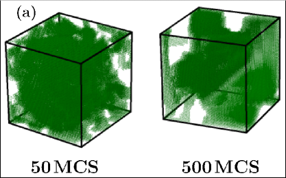
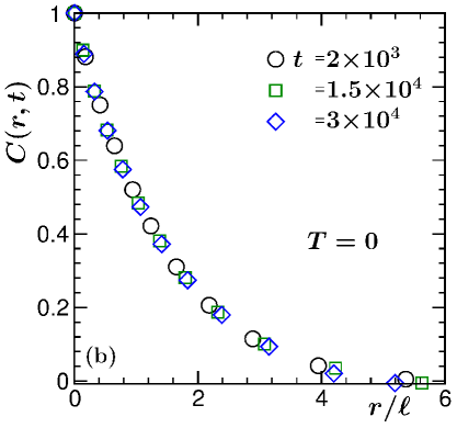
Figure 1: (a) Snapshots during the evolution of the 3D nonconserved Ising model. Pictures from two different times are shown. The locations of the “up” spins are marked. The linear dimension of the system is $L=64$. (b) Plots of two-point equal-time correlation function versus $r/\ell$. Data from three different times are included. The box size corresponds to $L=512$. All results are from $T=0$.

In Fig. 1(a) we show two snapshots during the evolution of the 3D Ising model, following a quench from infinite temperature to $T=0$. Growth in the system is clearly visible. To check for the structural self-similarity in the growth, in Fig. 1(b) we have plotted $C(r,t)$ versus $r/\ell$. Nice collapse of data from various different times imply the scaling propertybra :

$$C(r,t)=\tilde{C}(r/\ell(t)),$$ (10)

where $\tilde{C}(y)$ is independent of time, requirement for the self-similarity. While this qualitative feature is the same as that exhibited bra ; das by the model in $d=2$ or for quenches to much higher values of $T$ in $d=3$, we will later see that $\tilde{C}$ here differs from that for the latter cases. This feature may have important consequence in the aging property. Unless otherwise mentioned, all results below are for quenches to $T=0$. Here note that the collapse of the $C(r,t)$ from $t<1000$ on the presented data sets in Fig. 1(b) is not as good.

Next we focus our attention to the aging property. In Fig. 2 we present plots of $C_{\textrm{ag}}(t,t_{w})$ versus $t-t_{w}$, from three different values of $t_{w}$. As expected, no time translation invariance is observed zan and the decay becomes slower with the increase of $t_{w}$, implying aging in the system. However, the autocorrelation function for different $t_{w}$ values exhibit data-collapse when plotted versus $\ell/\ell_{w}$ dfish . This is demonstrated in Fig. 3. The solid line in this figure represents a power-law with exponent $\lambda=1.67$. This value was predicted by Liu and Mazenko (LM) liu , via a calculation that uses a Gaussian auxiliary field ansatz bra ; liu . LM constructed a dynamical equation for $C_{\textrm{gen}}(\vec{r}_{1},\vec{r}_{2},t,t_{w})$ as liu

$$\frac{\partial C_{\textrm{gen}}(\vec{R},t,t_{w})}{\partial t}={\nabla}^{2}C_{\textrm{gen}}(\vec{R},t,t_{w})+\frac{K}{t}C_{\textrm{gen}}(\vec{R},t,t_{w}),$$ (11)

where $\vec{R}=\vec{r}_{1}-\vec{r}_{2}$ and the constant $K$ depends upon $d$. The (approximate) solution of this equation, in the asymptotic limit, for $\vec{R}=0$, provides a power-law for $C_{\textrm{ag}}(t,t_{w})$:

$$C_{\textrm{ag}}(t,t_{w})\sim\ell^{-(d-2K)}.$$ (12)

Given that liu $K=0.6637$ in $d=3$, one obtains $\lambda=d-2K\simeq 1.67$.

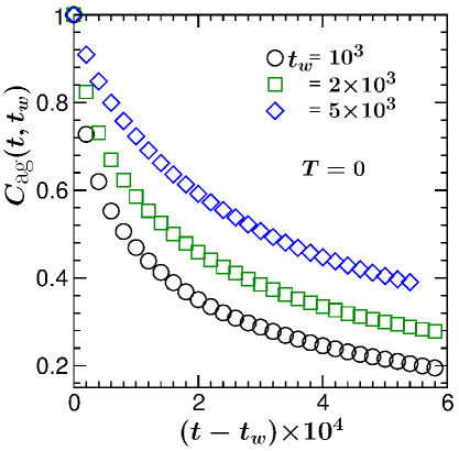
Figure 2: Plots of autocorrelation function versus $t-t_{w}$. Data from three different values of $t_{w}$ are shown. All results are for $T=0$ and $L=512$.

The LM line in Fig. 3, however, is in significant disagreement with the simulation data, even for very large value of $\ell$. Note that the presented data sets cover an overall length scale range $[50,250]$. However, as observed in previous studies in different dimension or at other temperatures, here also the scaling function exhibits continuous bending mid ; maj . Even though a fair agreement of the simulation data with the LM prediction is not yet observed, a trend for arriving at a better agreement with the latter or at least with a power-law behavior may be appreciated with the increase of $x=\ell/\ell_{w}$. This bending perhaps implies mid presence of correction(s) for smaller $x$.

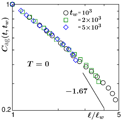
Figure 3: Scaling plot of $C_{\textrm{ag}}(t,t_{w})$ versus $\ell/\ell_{w}$, using data from three different values of $t_{w}$, on a log-log scale. The solid line represents a power-law, exponent being mentioned next to it. The presented results are from $T=0$ and $L=512$.

In such a situation, if indeed a power-law behavior is expected in the $x\rightarrow\infty$ limit, to estimate the exponent it is instructive to calculate the instantaneous exponent as mid ; hus

$$\lambda_{i}=-\frac{d\ln C_{\textrm{ag}}(t,t_{w})}{d\ln x}.$$ (13)

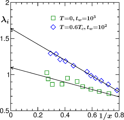
Figure 4: Plots of instantaneous exponent $\lambda_{i}$ versus $1/x$. We have presented data from $T=0$ and $0.6T_{c}$. The solid lines are guides to the eye. All results were obtained with $L=512$. We have done running averaging and thinned out data for the clarity of presentation. Oscillations in the $T=0$ data is due to strong fluctuations in each initial configurations.

We have calculated $\lambda_{i}$ for the scaling functions from $T=0$ and $T=0.6T_{c}$. These are plotted versus $1/x$ in Fig. 4. In both the cases linear convergence to the $x\rightarrow\infty$ limit is visible mid . Such an extrapolation for the $T=0.6T_{c}$ data indeed leads to a number that is consistent with the LM liu value $1.67$. Here note that in a later work cha2 , a modified value of $\lambda$, about $6\%$ smaller than $1.67$, was mentioned. On the other hand, for $T=0$ the convergence is to a much smaller value, $\simeq 1.1$. This number not only is significantly smaller than the LM dfish value, it also violates the FH (lower) bound by a huge margin. Here note that the linear trend exhibited by the data sets in Fig. 4 imply an exponential correction factor such that mid

$$C_{\textrm{ag}}(t,t_{w})=Ae^{-\frac{B}{x}}x^{-\lambda},$$ (14)

where $A$ and $B$ are constants.

At this point we recall a recent observation of structural differences ole ; ole2 of $T=0$ coarsening dynamics of 3D nonconserved Ising model with other situations. For that matter, in Fig. 5(a) we show a comparison of $C(r)$ at $T=0$ with that at $0.6T_{c}$. There exists significant difference between the two cases das . The one at $0.6T_{c}$ is in nice agreement with the OJK function (see the continuous line).

To understand the difference in the decay of $C_{\textrm{ag}}(t,t_{w})$ between the two chosen temperatures, we ask the question if the above mentioned structural mismatch is responsible for that. Here we note, Yeung, Rao and Desai (YRD) yeu mentioned that the FH bound should be valid for only nonconserved order-parameter dynamics. The latter type of dynamics, of course, is being studied in this paper. The above point is raised yeu by considering the known structural differences between conserved and nonconserved cases. Nevertheless, since, by now, we know that there exists difference between $T=0$ and higher temperature structures even within the nonconserved framework das ; ole ; ole2 , further discussion and results with respect to this is worth presenting.

YRD obtained a modified lower bound yeu

$$\lambda\geqslant\frac{d+\beta}{2},$$ (15)

where $\beta$ is the exponent for the small wave-vector ($k$) power-law behavior of structure factor [Fourier transform of $C(r,t)$] yeu2 :

$$S(k,t)\sim k^{\beta}.$$ (16)

In the case of usual nonconserved Ising dynamics $\beta=0$ and YRD bound coincides with the FH bound. Question now arises on the value of $\beta$ at $T=0$. Recall that there exists difference in $C(r,t)$ starting from intermediate length scale. This is consistent with the previous report that observed sponge-like structure ole ; ole2 . We also find holes inside the domains of “up” and “down” spins. See the two-dimensional cuts of the snapshots in Fig. 5(b), obtained from the evolutions following quenches to $T=0$ and $0.6T_{c}$. Essentially the domains of the two types of spins are inter-penetrating in an unusual manner, at $T=0$, and creating a porous structure. In that case we expect a different form of the $P(\ell_{d},t)$ at $T=0$ from that at $T=0.6T_{c}$. This is shown in Fig. 6(a). Even though the large $\ell_{d}$ behavior is exponential for both the temperatures (see the log-linear choice of the plots), indeed the small $\ell_{d}$ behavior is quite different in the two cases, due to the presence of the porousity at $T=0$. This feature is consistent with the above mentioned difference in $C(r,t)$. Such difference in $C(r,t)$ is expected to provide disagreement in small $k$ behavior of $S(k,t)$ between the two temperatures.

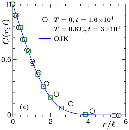
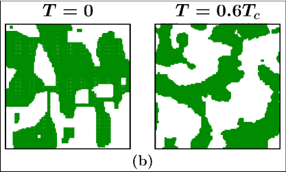
Figure 5: (a) A comparison of the two-point equal time correlation functions from $T=0$ and $0.6T_{c}$. In both the cases data from one time are presented, after scaling the distance axis by $\ell$. The continuous line there is the OJK analytical form. (b) Parts of 2D slices of snapshots from the evolutions at $T=0$ and $T=0.6T_{c}$. For $T=0.6T_{c}$, in the snapshot as well as for the calculation of $C(r,t)$ the thermal noise was removed (see the text).

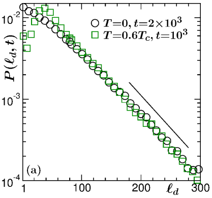
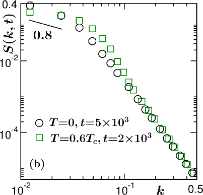
Figure 6: (a) Log-linear plots of the domain-size distribution function $P$ versus $\ell_{d}$. Results from $T=0$ and $0.6T_{c}$ are shown. The solid line represents an exponential decay. (b) Log-log plots of the equal-time structure factor vs $k$, at $T=0$ and $0.6T_{c}$. The solid line represents a power-law, exponent for which is mentioned. All results correspond to $L=512$. The times are mentioned in the figures and are chosen in such a way that the characteristic length scales at the two temperatures are approximately same.

In Fig. 6(b) we present log-log plots of $S(k,t)$ versus $k$, for the two chosen temperatures. The small $k$ behavior is certainly not consistent with $\beta=0$. However, for $T=0.6T_{c}$, value of $\beta$ is very close to zero ($\simeq 0.2$). (Note here that in $d=2$ or at high $T$ in $d=3$ various authors yeu ; yeu2 ; das confirmed that $\beta\simeq 0$.) For the validity of the YRD bound at $T=0$ one requires $\beta\simeq-0.8$. The small $k$ behavior of $S(k,t)$ at $T=0$ is reasonably consistent with this number – see the solid line in Fig. 6(b). We should mention here that for finite $L$ it is not possible to access very small values of $k$. If access of $k$ very close to zero becomes possible by considering large $L$, one may observe a behavior consistent with $\beta=0$ even for $T=0$, though such a convergence may be much slower than that for the higher temperature case. Furthermore, another question arises, what upper value of $k$ should be considered to be small. This can be answered by knowing the average domain size that grows with a slow rate at $T=0$. For this purpose we provide a brief discussion on how the YRD bound was obtained.

The derivation yeu of YRD bound required an integration over $k$ involving the structure factors at $t$ and $t_{w}$, viz.,

$$C_{\textrm{ag}}\sim\ell^{-\lambda}\leq\ell^{d/2}\int_{0}^{b}{dkk^{d-1}[{S(k,t_{w})}{\tilde{S}(k\ell)}]^{1/2}},$$ (17)

where $\tilde{S}$ is a time independent scaling function and $b=\frac{2\pi}{\ell}$, $\ell$ being the domain length at time $t$. The bound in Eq. (15) follows when $S(k,t_{w})$ in Eq. (17) is replaced by its small $k$ behavior as in Eq. (16). Given that the growth in the considered case is slow, value of $b$, i.e, the range of integration in $k$-space is bigger, at a given time, compared to higher temperature scenario where the growth is faster. This provides further larger “effective” value of $\beta$ in this case. Nevertheless, question remains, as mentioned above, with the increase of the system size a constant value of $S(k,t_{w})$ may be seen for $T=0$ and at very late time the value of $b$ may fall in that region. This will raise the value of the lower bound. In that case do we expect a crossover in the value of $\lambda$, from the value mentioned above, to the LM one? This will certainly be interesting to check. However, for that purpose, system sizes much larger than the ones considered here must be run for extremely long time. This exercise is not within our ability at the moment, given the limitation of computational resources available to us. Nevertheless, the system size $L=512$ studied in this work is extremely large and contains more than $0.13$ billion spins. To our knowledge, there exists only one study in the literature that considered comparable system size cor .

IV Conclusion

We have studied aging property zan during ordering in the 3D Ising model without conservation of order-parameter. Monte Carlo simulation lan results for quenches from infinite to zero temperature are presented for the two-time autocorrelation function. It has been shown, like in high temperature case mid , the decay of this correlation function, as a function of $x=\ell/\ell_{w}$, is a power-law, with an exponential correction for small $x$. The exponent for the power-law, however, is much smaller than that for the high temperature decay mid . While in the high $T$ case the exponent is consistent with a theoretical prediction by Liu and Mazenko liu , that obeys a lower bound provided by Fisher and Huse (FH) dfish , for $T=0$ this lower bound is violated. This is an extremely striking observation. Furthermore, the pattern at $T=0$ is different from that of the high temperature. For $T=0$, the Ohta-Jasnow-Kawasaki function oh does not describe the two-point equal-time correlation function well. The origin of this difference has been discussed. We argue, this deviation is responsible for the violation of the FH bound. In fact our result shows that the aging exponent obeys another bound, obtained by Yeung, Rao and Desai yeu , that can account for the structural anomaly mentioned above.

In this work the results from $T=0$ are compared with those from $0.6T_{c}$ that lies above the roughening transition temperature, $T_{R}$. In future we will perform more systematic study by gradually varying $T$. This will provide information on whether the surprising features that have been observed are only a zero temperature property or there is a gradual cross-over from $T=0$ to a higher temperature. This will also reveal if $T_{R}$, related to the interface broadening, is responsible for the unusual structure and dynamics.

${*}$ das@jncasr.ac.in

References

- (1) Onuki A. 2002 Phase Transition Dynamics (UK: Cambridge University Press)
- (2) Bray A.J. 2002 Adv. Phys. 51 481
- (3) Fisher D.S. and Huse D.A. 1988 Phys. Rev. B 38 373
- (4) Liu F. and Mazenko G.F. 1991 Phys. Rev. B 44 9185
- (5) Yeung C., Rao M. and Desai R.C. 1996 Phys. Rev. E 53 3073
- (6) Henkel M., Picone A. and Pleimling M. 2004 Europhys. Lett. 68 191
- (7) Lorentz E. and Janke W. 2007 Europhys. Lett. 77 10003
- (8) Midya J., Majumder S. and Das S.K. 2014 J. Phys.: Condens. Matter 26 452202
- (9) Midya J., Majumder S. and Das S.K. 2015 Phys. Rev. E 92 022124
- (10) Majumder S. and Das S.K. 2013 Phys. Rev. Lett. 111 055503
- (11) Zannetti M. in Kinetics of Phase Transitions (CRC Press, Boca Raton, 2009), ed. Puri S. and Wadhawan V.
- (12) Ohta T., Jasnow D. and Kawasaki K. 1982 Phys. Rev. Lett. 49 12223
- (13) Porod G. in Small-Angle X-ray Scattering, ed. Glatter O. and Kratky O. (Academic Press, New York, 1982)
- (14) Oono Y. and Puri S. 1988 Mod. Phys. Lett. B 2 861
- (15) Yeung C. 1988 Phys. Rev. Lett. 61 1135
- (16) Abraham D.B. and Upton P.J. 1989 Phys. Rev. B 39 736
- (17) Das S.K. and Chakraborty S. 2017 Eur. Phys. J. Special Topics 226 765
- (18) Shore J.D., Holzer M. and Sethna J.P. 1992 Phys. Rev. B 46 11376
- (19) Corberi F., Lippielo E. and Zannetti M. 2008 Phys. Rev. E. 78 011109
- (20) Olejarz J., Krapivsky P.L. and Redner S. 2011 Phys. Rev. E 83 051104
- (21) Olejarz J., Krapivsky P.L. and Redner S. 2011 Phys. Rev. E 83 030104
- (22) Chakraborty S. and Das S.K. 2016 Phys. Rev. E 93 032139
- (23) Majumdar S.N., Sire C., Bray A.J. and Cornell S.J. 1996 Phys. Rev. Lett. 77 2867
- (24) Derrida B. 1997 Phys. Rev. E 55 3705
- (25) Saharay M. and Sen P. 2003 Physica A 318 243
- (26) Blanchard T., Cugliandolo L.F. and Picco M. 2014 J. Stat. Mech.: Th. and Expt. P12021
- (27) Chakraborty S. and Das S.K. 2015 Eur. Phys. J. B 88 160
- (28) Mazenko G.F. 2004 Phys. Rev. E 69 016114
- (29) Allen S.M. and Cahn J.W. 1979 Acta Metall. 27 1085
- (30) Landau D.P. and Binder K. 2009 A Guide to Monte Carlo Simulations in Statistical Physics (UK: Cambridge University Press)
- (31) Huse D.A. 1986 Phys. Rev. B. 34 7845
- (32) Glauber R.J. 1963 J. Math. Phys. 4 294
- (33) van Beijeren H. and Nolden I., in Structure and Dynamics of Surface II: Phenomena, Models and Methods, Topics in Current Physics, ed. Schommers W. and von Blanckenhagen (Berlin: Springer)
- (34) Majumder S. and Das S.K. 2010 Phys. Rev. E 81 050102