A Stabilized bi-grid method for Allen Cahn equation in Finite Elements

Abstract

In this work, we propose a bi-grid scheme framework for the Allen-Cahn equation in Finite Element Method. The new methods are based on the use of two FEM spaces, a coarse one and a fine one, and on a decomposition of the solution into mean and fluctuant parts. This separation of the scales, in both space and frequency, allows to build a stabilization on the high modes components: the main computational effort is concentrated on the coarse space on which an implicit scheme is used while the fluctuant components of the fine space are updated with a simple semi-implicit scheme; they are smoothed without damaging the consistency. The numerical examples we give show the good stability and the robustness of the new methods. An important reduction of the computation time is also obtained when comparing our methods with fully implicit ones.

Hyam Abboud¹, Clara Al Kosseifi^2,3 and Jean-Paul Chehab²

¹Département de mathématiques, Faculté des Sciences II, Université Libanaise, Fanar, Liban

²Laboratoire Amiénois de Mathématiques Fondamentales et Appliquées (LAMFA), UMR CNRS 7352

Université de Picardie Jules Verne, 33 rue Saint Leu, 80039 Amiens France

³Laboratoire de Physique Appliquée (LPA), Faculté des Sciences II, Université Libanaise, Fanar, Liban

Keywords: Allen-Cahn equation, bi-grid method, stabilization, separation of the scales
     AMS Classification[2010]: 35N57,  65L07, 65M60,  65N55

1 Introduction

Phase fields equations, such as Allen-Cahn’s, are widely used in several domains of applied sciences for modeling natural phenomena in material science [3, 18], in image processing [25] or in ecology and in medicine [23], just to cite but a few. They are written as

$$\frac{\textstyle\partial u}{\textstyle\partial t}+M(-\Delta u+\frac{\textstyle 1}{\textstyle\epsilon^{2}}f(u))=0, x\in\Omega,t>0,$$ (1)

$$\frac{\textstyle\partial u}{\textstyle\partial\nu}=0,$$ (2)

$$u(0,x)=u_{0}(x),$$ (3)

where $\Omega$ is a bounded open set in $\mathbb{R}^{n}$ and $\nu$ the unit normal vector. The Allen-Cahn equation was introduced to describe the process of phase separation in iron alloys [4, 5], including order-disorder transitions: $M$ is the mobility (taken to be 1 for simplicity), $F=\displaystyle{\int_{-\infty}^{u}f(v)dv}$ is the free energy, $u$ is the (non-conserved) order parameter and $\epsilon>0$ is the interface length. The homogenous Neumann boundary condition implies that there is no loss of mass outside the domain $\Omega$. It is important to note that there is a competition between the potential term and the diffusion term: this produces a regularization in phase transition. This equation can be also viewed as a gradient flow for the energy $E(u)=\displaystyle\frac{\textstyle 1}{\textstyle 2}\int_{\Omega}\|\nabla u\|^{2}dx+\displaystyle\frac{\textstyle 1}{\textstyle\epsilon^{2}}\int_{\Omega}F(u)dx$. A generic and important consequence is that $\displaystyle\frac{\textstyle dE(u)}{\textstyle dt}\leq 0$, the energy is time-decreasing along the solutions, this is a stability property that is important to be recovered numerically; we refer the reader to recent works on numerical method for gradient flows applied to these equations [27].

The presence of the small parameter $\epsilon$ leads to numerical difficulties: it makes the functional $E(u)$ ”very non convex” in the sense that it possesses many local minima. Therefore, the use of semi-implicit methods suffers from a hard time step limitation while the use of implicit schemes allows to obtain energy diminishing methods but have an important cost in CPU time; however, as underlined in this paper, they present practical difficulties for their implementation. To combine the fast iterations of the semi-implicit schemes (only a linear problem has to be solved at each time step) and the good stability of the implicit schemes, stabilization methods have been considered, [28]. They are based on a $L^{2}$-like damping, but they can slow down the dynamics. This is attribuable to the fact that the damping acts on all the components, including on the low mode components of the solution which contains the main part of the information; the high mode components represent a fluctuant part that can play a crucial role for the numerical stability: indeed, the stability of a scheme lies on its capability to control their expansion.

Independently, bi-grid methods have been extensively studied for the solution of reaction-diffusion equation and also Navier-Stokes [1, 22]; they are based on the computation of an approximation of the solution on the coarse space $W_{H}$ by using an implicit scheme, the solution in the fine space $V_{h}$ is then obtained by applying a simplified yet semi-implicit scheme. A reduction of the CPU time is achieved, since the main computational effort is concentred only on a small system.

The aim of this article is to propose a framework of bi-grid methods in finite elements for the numerical approximation of the Allen-Cahn equations. The use of two grids, say of two FEM spaces $W_{H}$ and $V_{h}$ with $\mbox{dim}(W_{H})<<\mbox{dim}(V_{h})$, allows to build a scale separation (in space and in frequency) by decomposing the solution $u_{h}\in V_{h}$ as

$$u_{h}={\tilde{u}}_{h}+z_{h}.$$

Here ${\tilde{u}}_{h}={\cal P}(u_{H})$ is the $L^{2}$ prolongation in $V_{h}$ of $u_{H}$ (the approximation $u_{H}$ of the solution in $W_{H}$) is defined by

$$(u_{H}-{\cal P}(u_{H}),\phi_{h})=0,\forall\phi_{h}\in V_{h},$$

where $(.,.)$ denotes the scalar product in $L^{2}(\Omega)$. Hence ${\cal P}(u_{H})\in V_{h}$ represents the mean part of the solution; $z_{h}\in V_{h}$ is the fluctuant part and corresponds then to a small correction which carries the high frequencies. In that way, we can conjugate the bi-grid approach to reduce the CPU time and stabilize the correction step on the fine space by smoothing the fluctuant component. We consider the case $W_{H}\subset V_{h}$, in a such case the method is hierarchical-like but the framework is still valid when $W_{H}\not\subset V_{h}$.

The article is organized as follows: at first, in Section 2, we present briefly the phase fields problem (particularly the Allen-Cahn equation) and we recall the classical time marching schemes and their properties. After that, in Section 3, we introduce the bi-grid framework as well as the separation of the scales technique giving numerical illustrations. We then define the bi-grid scheme with the reference scheme on the coarse space and the correction scheme on the fine one. In section 4, we present numerical results on the Allen-Cahn equation emphasizing on the reduction of CPU time obtained by the new methods while the solutions fit with the ones computed with the classical schemes; we obtain particularly numerical evidences of the energy diminishing property for the new schemes. Finally, in Section 5, concluding remarks are given. All the numerical results were obtained using the free Finite Element software FreeFem++ [21].

2 Allen-Cahn equations, classical schemes. Advantages and limitations

The Allen-Cahn equation writes as

$$\frac{\textstyle\partial u}{\textstyle\partial t}-\Delta u+\varepsilon^{-2}f(u) =0,\ x\in\Omega,t\in(0,T),$$ (4)

$$\frac{\textstyle\partial u}{\textstyle\partial\nu}=0 \mbox{ on }\partial\Omega,t>0,$$ (5)

$$u(x_{0})=u_{0}(x) \mbox{ in }\Omega.$$ (6)

This equation can describe the separation of two phases, e.g; in a metal alloy; $\epsilon>0$ represents the width of the interface and $f=F^{\prime}$ is the derivative of the potential $F$. This system can be viewed also as a gradient flow for the energy $E(u)=\displaystyle\frac{1}{2}\displaystyle\int_{\Omega}|\nabla u|^{2}dx+\varepsilon^{-2}\displaystyle\int_{\Omega}F(u)dx$ and can be rewritten as

$$\frac{\textstyle\partial u}{\textstyle\partial t}+\nabla E(u)=0,$$

in such a way that $\displaystyle\frac{dE(u)}{dt}\leq 0$, which guarantees the stability of the system. This last property is very important and has to be satisfied at the discrete level to have (energy) stable time marching schemes; the maximum principle satisfied by the solution is another stability property (in $L^{\infty}$ norm). We refer to [8] for more details on the phase field modeling and on the mathematical properties of the solutions.

We now consider the time semi-discretization and focus on marching schemes. Let $u^{k}\simeq u(x,k\Delta t)$ be a sequence of functions; $\Delta t$ is the time step. We recall the following three classical schemes which will be used for building our new methods. Note that a scheme is energy diminishing when

$$E(u^{k+1})\leq E(u^{k}).$$

• Scheme 1: Semi Implicit scheme
  

  $$\frac{\textstyle u^{k+1}-u^{k}}{\textstyle\Delta t}-\Delta u^{k+1}+\frac{\textstyle 1}{\textstyle\varepsilon^{2}}f(u^{k}) =0, x\in\Omega,$$ (7)

  $$\frac{\textstyle\partial u^{k+1}}{\textstyle\partial\nu}=0, \mbox{ on }\partial\Omega.$$ (8)

  This scheme is energy diminishing: it is easy to implement (only a linear Neumann problem has to be solved at each step) but it suffers from a hard restrictive time step condition

  $$0<\Delta t<\frac{\textstyle 2\varepsilon^{2}}{\textstyle L},$$

  where $L=\|f^{\prime}\|_{\infty}$, see e.g., [28].

• Scheme 2: Implicit Scheme
  

  $$\frac{\textstyle u^{k+1}-u^{k}}{\textstyle\Delta t}-\Delta u^{k+1}+\frac{\textstyle 1}{\textstyle\varepsilon^{2}}DF(u^{k},u^{k+1}) =0, x\in\Omega,$$ (9)

  $$\frac{\textstyle\partial u^{k+1}}{\textstyle\partial\nu}=0, \mbox{ on }\partial\Omega,$$ (10)

  where we have set $DF(u,v)=\left\{\begin{array}[]{ll}\frac{\textstyle F(u)-F(v)}{\textstyle u-v}&\mbox{ if }u\neq v,\\ f(u)&\mbox{ if }u=v\end{array}\right.$.
  

  This scheme is unconditionally energy stable, i.e. energy diminishing for all $\Delta t>0$, see [16]. However it necessitates to solve a fixed point problem at each step.

• Scheme 3: Stabilized semi-implicit scheme
  A way to overcome the time step restriction while solving only one linear problem at each step is to add a stabilization term as follows [28]:

  $$\frac{\textstyle u^{k+1}-u^{k}}{\textstyle\Delta t}+\frac{\textstyle S}{\textstyle\varepsilon^{2}}(u^{k+1}-u^{k})-\Delta u^{k+1}+\frac{\textstyle 1}{\textstyle\varepsilon^{2}}f(u^{k}) =0, x\in\Omega,$$ (11)

  $$\frac{\textstyle\partial u^{k+1}}{\textstyle\partial\nu}=0, \mbox{ on }\partial\Omega.$$ (12)

  The scheme is energy diminishing for all $\Delta t>0$ when $S\geq\frac{\textstyle L}{\textstyle 2}$, see [28]. As the semi-implicit scheme, this method is easy to implement, however the stabilization slows down the dynamics. One can explain it as follows: the damping term $\frac{\textstyle S}{\textstyle\varepsilon^{2}}(u^{k+1}-u^{k})$ acts on all the modal components of the solution, the low ones that represents the main part of the solution and the high modes whose the limitation of the propagation allows to obtain the stability.

An effective numerical solution of the problem needs to have a fully discretized system, we consider here Finite Elements Method (FEM) for the space discretization. To develop an efficient scheme we have to take into account practical arguments, such as the implementation as well as the cost in CPU time.

Remark 2.1

The above list of time schemes is not exhaustive, let us cite the convex splitting scheme [20] which consist on decomposing the potential as a difference of a convex and an expansive term as $F(u)=F_{c}(u)-F_{e}(u)$. The scheme is then

$$\frac{\textstyle u^{k+1}-u^{k}}{\textstyle\Delta t}-\Delta u^{k+1}+\frac{\textstyle 1}{\textstyle\varepsilon^{2}}(\nabla F_{c}(u^{k+1})-\nabla F_{e}(u^{k}))=0.$$

Remark 2.2

An other important property of the solutions of Allen-Cahn’s equation is the maximum principle. For instance, when $f(u)=u(1-u^{2})$, it can be proved that if $|u_{0}(x)|\leq 1,\forall x\in\Omega$ then $|u(x,t)|\leq 1,\forall x\in\Omega,\forall t>0$: this is the $L^{\infty}$-stability.

3 Bi-grid framework

3.1 A scale separation in finite elements

As stated in the introduction, the high frequency components govern the stability of the scheme and the central idea of a stabilized scheme is to stop or to slow down their expansion. Of course, to this aim, we need to have a way to extract the high mode part of the solution to stabilize, say writing $u$ as

$$u={\tilde{u}}+z,$$ (13)

where ${\tilde{u}}$ is associated to the low mode part of $u$ and $z$, of small size; $z$ contains the high frequencies of $u$. This decomposition can be obtained by using several embedded approximation spaces, as in the hierarchical methods and nonlinear Galerkin methods [6, 14, 15, 26] and the references therein; however the embedding is not mandatory as shown hereafter. Let $V_{h}$ be the fine finite elements space and let $W_{H}$ be another FEM space with $\mbox{dim}(W_{H})<\mbox{dim}(V_{h})$. We define the prolongation operator ${\cal P}:W_{H}\rightarrow V_{h}$ by

$$(u_{H}-{\cal P}(u_{H}),\phi_{h})=0,\forall\phi_{h}\in V_{h}.$$ (14)

Note that is not necessary to have $W_{H}\subset V_{h}$ which means that we can avoid the building of a hierarchical basis and then the method can be considered for many FEM spaces. However, it is important to have compatibility conditions on $W_{H}$ and $V_{h}$ in such a way the prolongation is uniquely defined. Let $(\phi_{i})_{i=1}^{N}$ and $(\psi_{j})_{j=1}^{M}$ be two bases of $V_{h}$ and of $W_{H}$ respectively ($M<N$). We define the matrix $B_{H}^{h}$ as $(B_{H}^{h})_{i,j}=(\phi_{i},\psi_{j}),\ i=1,\cdots,N,\ \ j=1,\cdots,M$. The prolongation step writes as

$$M_{h}{\cal P}(u_{H})=B_{H}^{h}u_{H}.$$

Hence, since $M_{h}$ is a mass matrix, ${\cal P}(u_{H})$ is uniquely defined whenever the rank of $B_{H}^{h}$ is maximal, say equal to $M$. Of course this condition is automatically satisfied when $W_{H}\subset V_{h}$.
We give hereafter a sufficient condition for the injectivity of $B_{H}^{h}$:

Proposition 3.1

Let $W_{H}$ and $V_{h}$ be two FEM spaces built on ${\cal C}^{0}$ reference elements. Assume that $\forall u_{H}\in W_{H},\left((u_{H},\phi_{h})=0,\forall\phi_{h}\in V_{h}\Rightarrow u_{H}=0\right)$ Then, $B_{H}^{h}$ is injective. Moreover, there exists two constants $\beta$ and $\alpha_{H}^{h}>0$ such that $0<\alpha_{H}^{h}<\beta\leq 1$ and

$$\alpha_{H}^{h}\|u_{H}\|\leq\|{\cal P}(u_{H})\|\leq\beta\|u_{H}\|,\forall u_{H}\in W_{H}.$$

Proof. The assumption implies that if ${\cal P}(u_{H})=0$, then $(u_{H},\phi_{h})=0,\ \forall\phi_{h}\in V_{h}$, then $u_{H}=0$ which gives the injectivity.

Now assuming that ${\cal P}(u_{H})\neq 0$ and taking $\phi_{h}={\cal P}(u_{H})$ in (14), we find

$$\|{\cal P}(u_{H})\|^{2}=({\cal P}(u_{H}),u_{H})=\frac{\textstyle({\cal P}(u_{H}),u_{H})}{\textstyle\|u_{H}\|\|{\cal P}(u_{H})\|}\|u_{H}\|\|{\cal P}(u_{H})\|.$$

Let $\alpha_{H}^{h}=\inf_{u_{H}\in W_{H}}\frac{\textstyle({\cal P}(u_{H}),u_{H})}{\textstyle\|u_{H}\|\|{\cal P}(u_{H})\|}$. We now show that $\alpha_{H}^{h}>0$. We can write

$$\alpha_{H}^{h}=\inf_{u_{H}\in W_{H},\|u_{H}\|=1}({\cal P}(u_{H}),u_{H})\geq 0.$$

The function $u_{H}\in W_{H}\mapsto({\cal P}(u_{H}),u_{H})\in\mathbb{R}^{+}$ is obviously continuous on the compact set ${\cal B}=\{u_{H}\in W_{H},\|u_{H}\|=1\}$. Its minimum is reached and can not be equal to $0$ because $0$, the only root, is outside ${\cal B}$. Hence $\alpha_{H}^{h}>0$ and we infer from above that

$$\|{\cal P}(u_{H})\|\geq\alpha_{H}^{h}\|u_{H}\|\geq 0.$$

Now, in the same way, we have

$$\|{\cal P}(u_{H})\|^{2}=({\cal P}(u_{H}),u_{H})=\frac{\textstyle({\cal P}(u_{H}),u_{H})}{\textstyle\|u_{H}\|\|{\cal P}(u_{H})\|}\|u_{H}\|\|{\cal P}(u_{H})\|.$$

But, as a consequence of the Cauchy-Schwarz inequality,

$$\frac{\textstyle({\cal P}(u_{H}),u_{H})}{\textstyle\|u_{H}\|\|{\cal P}(u_{H})\|}\leq 1,$$

so $\beta=\sup_{u_{H}\in W_{H},\|u_{H}\|=1}({\cal P}(u_{H}),u_{H})\leq 1$. Finally

$$\alpha_{H}^{h}\|u_{H}\|\leq\|{\cal P}(u_{H})\|\leq\beta\|u_{H}\|,\forall u_{H}\in W_{H}.$$

 

Remark 3.2

These conditions mean that the range of the angles between the elements of $W_{H}$ and those of ${\cal P}(W_{H})\subset V_{h}$ is in the interval $[\arccos(\beta),\arccos{\alpha_{H}^{h}}]$; the condition $\alpha_{H}^{h}>0$ avoids situations of orthogonality. Of course $\alpha_{H}^{h}$ can depend on $H$ and $h$ and can become smaller and smaller as $H$ and $h$ go to $0$. The best situation being when $\alpha_{H}^{h}$ is independent of both $h$ and $H$.

The correction $z$ is defined on the whole fine space $V_{h}$ and not on a complementary space. Of course, one expect $z$ to be a correction (i.e. small in norm) for regular functions $u$. More precisely, we have the following result:

Proposition 3.3

Let $W_{H}$ and $V_{h}$ be two FEM spaces that we assume to be of class ${\cal C}^{0}$ and associated to nested regular triangulations of $\Omega$, a regular bounded open set of $\mathbb{R}^{n}$; $(K,P,\Sigma)$ is the reference element. For $u\in H^{k+1}(\Omega)$, we denote by $u_{h}=\Pi_{h}u$ and $u_{H}=\Pi_{H}u$ the P-interpolate of $u$ in $V_{h}$ and $V_{H}$ respectively. We assume that $P_{k}\subset P$. We have the following estimate:

$$\|u_{h}-{\cal P}u_{H}\|_{L^{2}(\Omega)}\leq CH^{k+1}\|u\|_{H^{k+1}(\Omega)}.$$

Proof. We start from the classical interpolation error estimates in FE spaces [19],

$$\|u-\Pi_{h}u\|_{L^{2}(\Omega)}\leq Ch^{k+1}\|u\|_{H^{k+1}(\Omega)}\mbox{ and }\|u-\Pi_{H}u\|_{L^{2}(\Omega)}\leq CH^{k+1}\|u\|_{H^{k+1}(\Omega)}.$$

We can write

$$u_{h}-{\cal P}(u_{H})=u_{h}-u+u-u_{H}+u_{H}-{\cal P}(u_{H}),$$

hence

$$(u_{h}-u+u-u_{H}+u_{H}-{\cal P}(u_{H}),\phi_{h})=(u_{h}-u+u-u_{H},\phi_{h}),\forall\phi_{h}\in V_{h}.$$

Taking $\phi_{h}=u_{h}-{\cal P}(u_{H})\in V_{h}$, we find,

$$\|u_{h}-{\cal P}(u_{H})\|^{2}_{L^{2}(\Omega)}\leq\|u_{h}-u+u-u_{H}\|_{L^{2}(\Omega)}.\|u_{h}-{\cal P}(u_{H})\|_{L^{2}(\Omega)},$$

then

$$\|u_{h}-{\cal P}(u_{H})\|_{L^{2}(\Omega)}\leq\|u_{h}-u+u-u_{H}\|_{L^{2}(\Omega)}\leq\|u_{h}-u\|_{L^{2}(\Omega)}+\|u_{H}-u\|_{L^{2}(\Omega)}.$$

Finally

$$\|u_{h}-{\cal P}(u_{H})\|_{L^{2}(\Omega)}\leq C^{\prime}H^{k+1}\|u\|_{H^{k+1}(\Omega)},$$

where $C^{\prime}>0$ is independent of $h,H$ and $u$.   

Remark 3.4

For $0\leq m\leq k+1$, defining ${\cal P}$ as $({\cal P}(u_{H})-u_{H},\phi_{h})_{m}=0,\forall\phi_{h}\in V_{h}$, where $(.,.)_{m}$ is the standard scalar product in $H^{m}$, then, proceeding as above, we can prove that

$$\|u_{h}-{\cal P}(u_{H})\|_{H^{m}(\Omega)}\leq CH^{k+1-m}\|u\|_{H^{k+1}(\Omega)}.$$

3.2 Illustration

For given functions and finite elements spaces $P_{1}$ and $P_{2}$, we build the decomposition (13)-(14). We generate the meshes with FreeFem++ [21] using Delaunay’s triangulation starting from the boundary. We have taken $Nf=100$ boundary points for generating ${\cal T}_{h}$, the mesh associated to the fine space $V_{h}$ and $Nc=50$ boundary points for generating ${\cal T}_{H}$, the mesh associated to the coarse space $W_{H}$. The first example is the decomposition of the function $u(x,y)=(x^{2}+y^{2}-1)(x^{2}+y^{2}-4)$ on the torus; the second one is with $u(x,y)=\sin(72x(1-x)y(1-y))$ on the unit square. Below, in Figure 1 and Figure 2, we observe that the $z$ component are much smaller in magnitude than those of the original function ($10\%$ for $P_{1}$ and $0.5\%$ for $P_{2}$ elements).

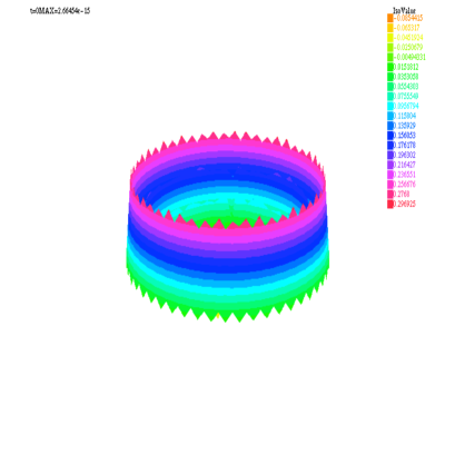
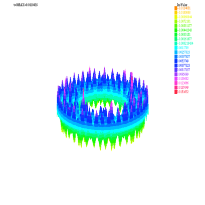
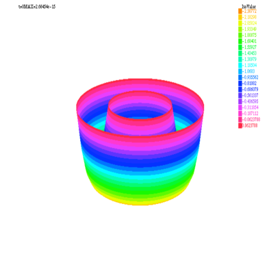
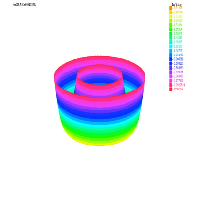
Figure 1: Correction components for $u(x,y)=(x^{2}+y^{2}-1)(x^{2}+y^{2}-4)$, 3d output and iso-values, $P_{1}$ elements

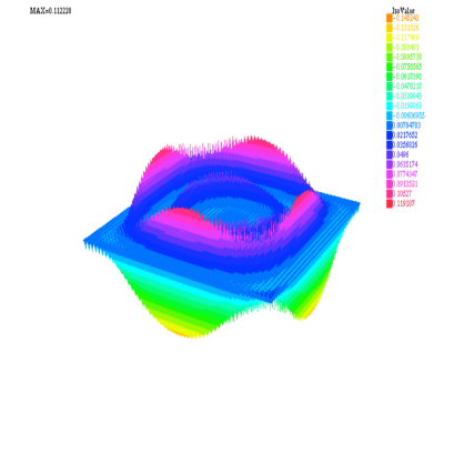
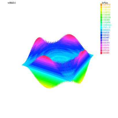
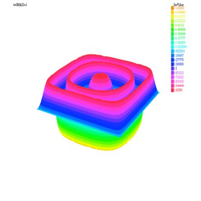
Figure 2: Correction components for $u(x,y)=\sin(72x(1-x)y(1-y))$, 3d output and isovalues, $P_{1}$ elements

Remark 3.5

The same can be done with Neumann Boundary Conditions (B.C.) that are the usual B.C. for the Allen-Cahn equation on which we will concentrate now.

In the previous figures we have illustrated the effect of the scale separation in space: the fluctuant part of the function, $z$, is small in amplitude as respected to the one of the original function. This is observed when considering $P_{1}$ as well as $P_{2}$ elements. We observe also that the $z$-component exhibit high oscillations that are characteristic to the high frequency part of a function. We now quantify this property.
We generate the approximations of the eigenfunction in the FEM space by solving numerically eigenvalues problem,

$$\int_{\Omega}u_{h}v_{h}dx+\int_{\Omega}\nabla u_{h}\nabla v_{h}dx=\lambda\int_{\Omega}u_{h}v_{h}dx \forall v_{h}\in V_{h},$$ (15)

which is equivalent to find the eigen-elements of

$$A_{h}u=\lambda M_{h}u,$$ (16)

where $A_{h}$ and $M_{h}$ are respectively the stiffness and the mass matrix on the FEM space $V_{h}$. Denote by $(w^{(i)},\lambda_{i})$ the eigenvectors associated to the eigenvalue $\lambda_{i}$, we compare the first eigen-components of $U$ and those of $Z$ to point out, that is

$$\int_{\Omega}Uw^{(i)}dx\mbox{ and }\int_{\Omega}Zw^{(i)}dx.$$

In Figures 3 and 4, we have represented the energy spectrum of $u(x,y)=\cos(44(1-x)xy(1-y))$ and of its fluctuant component $z$, when using $P_{2}$ as well as $P_{1}$ elements. We observe that the low mode components of $z$ are reduced in an important way as respected to the ones of $u$ while the high modes components are less smoothed; hence $z$ carries the high frequencies.

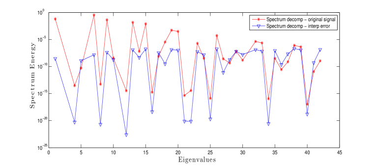
Figure 3: $P2$ FEM, $u(x,y)=\cos(44(1-x)xy(1-y))$, $\mbox{dim}(V_{h})=1681,\ \mbox{dim}(W_{H})=441$

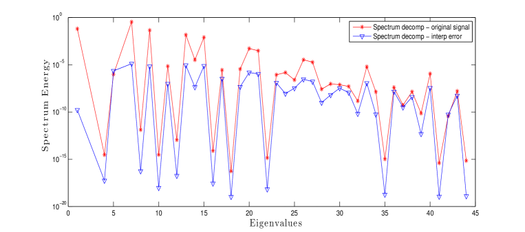
Figure 4: $P1$ FEM, $u(x,y)=\cos(44(1-x)xy(1-y))$, $\mbox{dim}(V_{h})=1681,\ \mbox{dim}(W_{H})=441$

3.3 The bi-grid framework

Algorithm 1 Scheme 4: Bi-grid scheme

1:for $k=0,1,\cdots$ do

2:

3:     Solve in $W_{H}$ ($\displaystyle\frac{u_{H}^{k+1}-u_{H}^{k}}{\Delta t},\psi_{H})+(\nabla u_{H}^{n+1},\nabla\psi_{H})+(DF(u^{k+1}_{H},u^{k}_{H}),\psi_{H})=0,\forall\psi_{H}\in V_{H}$

4:     Solve in $V_{h}$ $(\tilde{u}_{h}^{k+1},\phi_{h})-(u_{H}^{k+1},\phi_{h})=0,\forall\phi_{h}\in V_{h}$

5:     Solve

$$\begin{array}[]{ll}\vskip 6.0pt plus 2.0pt minus 2.0pt(1+\tau\Delta t)(z_{h}^{k+1}-z_{h}^{k},\phi_{h})+\Delta t(\nabla z_{h}^{k+1},\nabla\phi_{h})+\Delta t(\nabla\tilde{u}_{h}^{k+1},\nabla\phi_{h})\\ \vskip 6.0pt plus 2.0pt minus 2.0pt+(\tilde{u}_{h}^{k+1}-\tilde{u}_{h}^{k},\phi_{h})+\Delta t({\tilde{f}}(u_{h}^{k},{\tilde{u}}_{h}^{k+1},z_{h}^{k+1}),\phi_{h})=0,\forall\phi_{h}\in V_{h}\\ \end{array}$$

6:     Set $u^{k+1}=\tilde{u}_{h}^{k+1}+z_{h}^{k+1}$

7:end for

Here ${\tilde{f}}(u^{k},{\tilde{u}}^{k+1}_{h},z_{h}^{k+1})$ is an approximation of $f(u^{k+1}_{h})$, e.g. ${\tilde{f}}(u^{k},{\tilde{u}}^{k+1}_{h},z_{h}^{k+1})=f(u^{k}_{h})$. For this choice of ${\tilde{f}}$ we have an important property: the high mode stabilization makes the bi-grid scheme consistent with the computation of the steady states. More precisely, we have

Proposition 3.6

Assume, for fixed $h$ and $H$, that there exists a unique pair of elements ${\bar{u}}_{H}\in W_{H}$ and ${\bar{u}}_{h}\in V_{h}$ such that

$$(\nabla{\bar{u}}_{H},\nabla\psi_{H})+(f({\bar{u}}_{H}),\psi_{H})=0,\forall\psi_{H}\in W_{H}\mbox{ and }(\nabla{\bar{u}}_{h},\nabla\phi_{h})+(f({\bar{u}}_{h}),\phi_{h})=0,\forall\phi_{h}\in V_{h}.$$

Assume that $\lim_{k\rightarrow+\infty}u_{H}^{k}={\bar{u}}_{H}$ and that $z^{k}_{h}$ is convergent to ${\bar{z}}_{h}$. Then

$$\mbox{ and }\lim_{k\rightarrow+\infty}u_{h}^{k}={\bar{u}}_{h}.$$

Proof. To establish the consistency, we show that $u^{k}_{h}=z^{k}_{h}+{\tilde{u}}^{k}_{h}$ converges to ${\bar{u}}_{h}$.
By continuity of the prolongation ${\cal P}$, we have

$${\cal P}(u^{n}_{H})={\tilde{u}}_{h}^{k}\rightarrow{\cal P}({\bar{u}}_{H})={\tilde{\bar{u}}}_{h},\mbox{ as }k\rightarrow+\infty.$$

Taking the limit in the correction step of the scheme, we get, after the usual simplifications

$$(\nabla z_{h},\nabla\phi_{h})+(\nabla\tilde{u}_{h},\nabla\phi_{h})+(f(z_{h}+{\tilde{u}}_{h}),\phi_{h})=0,\forall\phi_{h}\in V_{h}.$$

Letting $w_{h}=z_{h}+{\tilde{u}}_{h}$, we find

$$(\nabla w_{h},\nabla\phi_{h})+(f(w_{h}),\phi_{h})=0,\forall\phi_{h}\in V_{h}.$$

By identification, $w_{h}=z_{h}+{\tilde{u}}_{h}={\bar{u}}_{h}$.   

4 A big-grid method for Allen-Cahn Equation

As presented above, the bi-grid scheme is based on an implicit (stable) scheme applied on the coarse space $W_{H}$ and on a simplified semi-implicit scheme on the fine space $V_{h}$, for the computation of the correction (fluctuant) term $z$. The scheme on $W_{H}$ is considered to be the reference scheme. Its implementation necessitates the numerical solution of a fixed point problem at each time step. We present hereafter a way to overcome the artificial instability carried by the use of the classical Picard iterates. The new nonlinear iterations will be implemented to define the effective reference scheme when applied to $V_{h}$ and to which we will compare the bi-grid schemes.

4.1 A solution to an artificial instability problem for a one-grid scheme

The implementation of the scheme (9) needs a fixed point problem to be solved at each time step. Let $M_{h}$ and $A_{h}$ be the mass and the stiffness matrices respectively. If we set

$$\phi(v,u^{k})=\Big{(}M_{h}+\Delta tA_{h}\Big{)}^{-1}\Big{\{}u^{k}-\displaystyle\frac{\Delta t}{\epsilon^{2}}DF(u^{k},v)\Big{\}},$$

then the time marching scheme reduces to solve the fixed point problem

$$v=\phi(v,u^{k})$$ (17)

at the n^th time step. In practice, the convergence of the Picard iterates is obtained by taking only very small values of $\Delta t$, typically $\Delta t\simeq 10^{-4}$. This is dramatic since we are looking to the long time numerical behavior of the solution. Anyway, this effective restriction on the time step is really artificial because the scheme is supposed to be unconditionally stable. For this reason, as in [2] (in the Nonlinear Schrödinger Equation case), we apply here the extrapolation of the fixed point to compute $u^{k+1}$ from $u^{k}$ and we propose to solve (17) by accelerating the (Picard) sequence

$$\left.\begin{array}[]{ll}\vskip 6.0pt plus 2.0pt minus 2.0ptv^{0}=u^{n},\\ \vskip 6.0pt plus 2.0pt minus 2.0pt\text{for}\;\;m=0,\ldots\\ \vskip 6.0pt plus 2.0pt minus 2.0ptv^{(m+1)}=\phi(v^{(m)},u^{k}),\end{array}\right.$$ (18)

enhancing in that the stability region, allowing then to take larger values of $\Delta t$. To this end, we use the $\Delta^{\kappa}$ acceleration procedure, see [9]. In two words, the $\Delta^{\kappa}$ procedure consists in replacing the Picard iterates by

$$\left.\begin{array}[]{ll}\vskip 6.0pt plus 2.0pt minus 2.0ptv^{0}=u^{k},\\ \vskip 6.0pt plus 2.0pt minus 2.0pt\text{for}\;\;m=0,\ldots\\ \vskip 6.0pt plus 2.0pt minus 2.0ptv^{(m+1)}=v^{(m)}-(-1)^{\kappa}\alpha_{m}^{\kappa}\Delta_{\phi}^{k}v^{(m)};\end{array}\right.$$ (19)

where $\Delta_{\phi}^{\kappa}v^{(m)}=\displaystyle\sum_{j=0}^{\kappa}C_{j}^{\kappa}(-1)^{\kappa-j}\phi^{(j)}(v^{(m)},u^{k}),\;C_{j}^{\kappa}=\displaystyle\frac{\kappa!}{j!(\kappa-j)!}$ is the binomial c$\oe$fficient and $\phi^{(j)}$ denotes the $j^{th}$ composition of $\phi$ with itself. We have

$$\alpha_{m}^{\kappa}=(-1)^{\kappa}\displaystyle\frac{<\Delta_{\phi}^{1}v^{(m)},\Delta_{\phi}^{\kappa+1}v^{(m)}>}{<\Delta_{\phi}^{\kappa+1}v^{(m)},\Delta_{\phi}^{\kappa+1}v^{(m)}>},$$ (20)

where $<.,.>$ denotes the euclidean scalar product in $\mathbb{R}^{n}$, see [9]. These acceleration procedures have been applied with the $\Delta^{1}$ (Lemaréchal’s method[24] corresponding to $\kappa=1$); we can take $\Delta t=10^{-2}$ and the scheme (9) is still stable. A comparison of the energy curves shows a digital convergence by varying the number of nodes on the edge of the unit square $N$ to generate the mesh ${\cal T}_{h}$, for $\epsilon=0.03$ and Lemaréchal’s acceleration.

Figure 5: Energy curves for $N=30\ (\mbox{dim}(V_{h})=961),N=40\ (\mbox{dim}(V_{h})=1681),N=80\ (\mbox{dim}(V_{h})=6561)$ on the unit square with $P_{1}$ element, $\Delta t=0.009$ and Lemaréchal method.

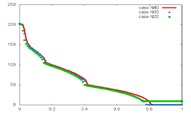
Figure 6: Energy curves for $N=20\ (\mbox{dim}(V_{h})=1681),N=30\ (\mbox{dim}(V_{h})=3721),N=40\ (\mbox{dim}(V_{h})=6561)$ on the unit square with $P_{2}$ element, $\Delta t=10^{-2}$ and Lemaréchal method.

The efficiency of this method appears in reducing the number of internal iterations required to reach a final time $T$. We present the CPU computation time and the number of internal iterations following the numerical implementation done on the unit square for $T=0.4$ and the maximum time step respectively for Lemaréchal and Picard method.

Case P2 Picard $$\Delta t=3\times 10^{-4}$$ T=0.4 Nb iter=34266 CPU=2851.62s

N=20 Lemarechal T=0.4 Nb iter=360 CPU=73.595s

Case P2 Picard T=0.4 Nb iter=34796 CPU=11639.8s

N=40 Lemarechal T=0.4 Nb iter=1600 CPU=1598.8s

Case P2 Picard T=0.4 Nb iter=35142 CPU=47686.2s

N=80 Lemarechal T=0.4 Nb iter=1599 CPU=11250.5s

4.1.1 Numerical results

In order to compare the two fixed point methods, we present below the evolution curve of the functional energy over time and some numerical results for the unconditionally stable scheme (9) by using the mesh of the unit square with $N=40$, the initial condition $u_{0}=\cos(4\pi x)\cos(4\pi y)$, the interfacial width $\epsilon=0.03$, $\Delta t=10^{-4}$ and the finite element $P_{2}$.

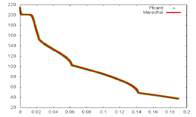
Figure 7: Energy curves for Picard and for Lemaréchal.

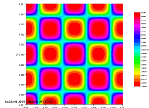
Figure 8: Picard (left) and Lemaréchal (Right) at $t=0.0059$.

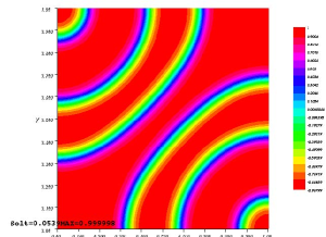
Figure 9: Picard (left) and Lemaréchal (Right) at $t=0.0539$.

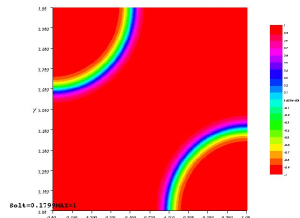
Figure 10: Picard (left) and Lemaréchal (right) at $t=0.1799$.

4.2 How to choose $W_{H}$ and $V_{h}$

A central question for the bi-grid method is the choice of the two approximation spaces $W_{H}$ and $V_{h}$. We have to balance two criteria:

• the CPU reduction capabilities brought by the bi-grid scheme: the most important part of the computations is realized in the coarse space (nonlinear iterations). This is directelty related to the ratio of the dimensions of $W_{H}$ and $V_{h}$, that we denote by $DR=\frac{\textstyle\mbox{dim($W_{H}$)}}{\textstyle\mbox{dim($V_{h}$)}}$.

• the scale separation in frequency that allows to make a correction through a simplified scheme on $V_{h}$. It appears that a good indicator is that the fine space correction term $z$ is in norm, this means that the approximation on the coarse space is sufficiently correct to be an acceptable approximation on the fine space once prolongated. According to the general case, see Proposition 3.3, an indicator of the $L^{2}$ norm of $z$ is controlled by the interpolation error in $W_{H}$.

Estimates on the relative step size of $W_{H}$ and $V_{h}$ in the case $W_{H}\subset V_{h}$ have been obtained in different contexts, see [26, 29] for bi-grid Nonlinear Galerkin (reaction-diffusion problem) and [1] for Navier-Stokes time dependent equations.

Here the condition $W_{H}\subset V_{h}$ is not mandatory and we can then define a mixed finite element scheme, the compatibillty condition between the FEM is given in proposition 3.1.

We give hereafter possible choices for $W_{H}$ and $V_{h}$ in several situations:

• The case $W_{H}\subset V_{h}$

  • When ${\cal T}_{H}={\cal T}_{h}$:

    $$W_{H}=\{v_{h}\in{\cal C}^{0}({\bar{\Omega}}),v_{h}|_{K}\in P_{p},\forall K\in{\cal T}_{h}\},\ V_{h}=\{v_{h}\in{\cal C}^{0}({\bar{\Omega}}),v_{h}|_{K}\in P_{q},\forall K\in{\cal T}_{h}\},$$

    with $q>p$. For instance $p=1,q=2$ or $q=3$.
    
    Following Proposition 3.3, it is easy to see that

    $$\|u-\Pi_{h}u\|_{L^{2}(\Omega)}\leq Ch^{q+1}\|u\|_{H^{q+1}(\Omega)}\mbox{ and }\|u-\Pi_{H}u\|_{L^{2}(\Omega)}\leq Ch^{p+1}\|u\|_{H^{p+1}(\Omega)},$$

    so the a priori optimal estimation for the prolongation error is $H^{p+1}$.

  • When ${\cal T}_{H}\subset{\cal T}_{h}$:

    $$W_{H}=\{v_{h}\in{\cal C}^{m}({\bar{\Omega}}),v_{h}|_{K}\in P_{p},\forall K\in{\cal T}_{h}\},\ V_{h}=\{v_{h}\in{\cal C}^{m}({\bar{\Omega}}),v_{h}|_{K}\in P_{p},\forall K\in{\cal T}_{h}\}.$$

    Another way to build $W_{H}$ from $V_{h}$ is to apply a coarsening procedure, we refer the reader e.g. to [7].

• The case $W_{H}\not\subset V_{h}$: the a priori estimates given by Proposition 3.3 still holds and the relation $H^{p+1}\simeq h^{q+1}$ gives an indication to choose the relative step sizes $h$ and $H$ of ${\cal T}_{H}$ and ${\cal T}_{h}$ . As above, the condition $h\textless\textless H$ is necessary to expect a CPU time reduction.

Remark 4.1

We focus here on $P_{k}$ elements but the bi-grid method could apply to FEM spaces built with rectangular or cubic elements $Q_{k}$.

4.3 Two-grid schemes for Allen-Cahn Equation

We now present two bi-grid schemes based on two different choices of ${\tilde{f}}(u_{h}^{k},{\tilde{u}}_{h}^{k+1},z_{h}^{k+1})$ in the case $f(u)=u(u^{2}-1)$:

• ${\tilde{f}}(u_{h}^{k},{\tilde{u}}_{h}^{k+1},z_{h}^{k+1})=f(u^{k}_{h})$: the correction step of the bi-grid scheme is a simple high mode stabilization of the semi-implicit scheme. This choice defines the Scheme 4.1 presented below.

• Linearization for the nonlinear term:

  $$\begin{array}[]{ll}{\tilde{f}}(u_{h}^{k},{\tilde{u}}_{h}^{k+1},z_{h}^{k+1})&=\frac{\textstyle 1}{\textstyle 4\epsilon^{2}}(u_{h}^{k}+2\tilde{u}_{h}^{k+1}u_{h}^{k}+3\tilde{u}_{h}^{k+1}-2)z_{h}^{k+1}\\ &+\frac{\textstyle 1}{\textstyle 4\epsilon^{2}}((\tilde{u}_{h}^{k+1})^{2}+(u_{h}^{k})^{2}-2)(\tilde{u}_{h}^{k+1}+u_{h}^{k}).\end{array}$$

  This choice defines the Scheme 4.2 presented below.

Algorithm 2 Scheme 4.1: Two-grid Stabilized Allen-Cahn equation with correction

1:$u_{h}^{0},u^{0}_{H}$ given

2:

3:for $k=0,1,\cdots$ do

4:     Solve $(u^{k+1}_{H},\psi_{H})+\Delta t(\nabla u_{H}^{k+1},\nabla\psi_{H})=(u^{k}_{H},\psi_{H}),\;\forall\psi_{H}\in W_{H}$

5:           $+\Delta t\frac{\textstyle 1}{\textstyle\epsilon^{2}}(DF(u_{H}^{k+1},u_{H}^{k}),\psi_{H})$

6:     Solve $({\tilde{u}}^{k+1}_{h}-u_{H}^{k+1},\phi_{h})=0,\;\forall\phi_{h}\in V_{h}$

7:     Solve $(1+\tau\Delta t)(z^{k+1}_{h},\phi_{h})+\Delta t(\nabla z^{k+1}_{h},\nabla\phi_{h})=(1+\tau\Delta t)(z^{k}_{h},\phi_{h})$

8:                                                $-\Delta t(\nabla{\tilde{u}}_{h}^{k+1},\nabla\phi_{h})-({\tilde{u}}^{k+1}_{h}-{\tilde{u}}^{k}_{h},\phi_{h})$

9:                                                $-\frac{\textstyle\Delta t}{\textstyle 4\epsilon^{2}}(u_{h}^{k}((u^{k})^{2}-1),\phi_{h})\forall\phi_{h}\in V_{h}$

10:     Set $u_{h}^{k+1}={\tilde{u}}_{h}^{k+1}+z_{h}^{k+1}$

11:end for

Remark 4.2

It is important to note that the above scheme can be implemented very simply without computing explicitly the sequence $z^{k}_{h}$: indeed, we can rewrite the correction step as

$$\begin{array}[]{ll}(u^{k+1}_{h},\phi_{h})&\\ +\Delta t\tau(u^{k+1}_{h}-u^{k}_{h},\phi_{h})&=(u^{k}_{h},\phi_{h})+\Delta t\tau(u^{k+1}_{H}-u^{k}_{H},\phi_{h})-\Delta t\frac{\textstyle 1}{\textstyle\epsilon^{2}}(f(u_{h}^{k}),\phi_{h}),\;\forall\phi_{h}\in V_{h}.\\ +\Delta t(\nabla u_{h}^{k+1},\nabla\phi_{h})&\end{array}$$

Algorithm 3 Scheme 4.2: Two-grid Stabilized Allen-Cahn equation with correction

1:$u_{h}^{0},u^{0}_{H}$ given

2:

3:for $k=0,1,\cdots$ do

4:     Solve $(u^{k+1}_{H},\psi_{H})+\Delta t(\nabla u_{H}^{k+1},\nabla\psi_{H})=(u^{k}_{H},\psi_{H}),\;\forall\psi_{H}\in W_{H}$

5:           $+\Delta t(\frac{\textstyle 1}{\textstyle\epsilon^{2}}DF(u_{H}^{k+1},u_{H}^{k}),\psi_{H})$

6:     Solve $({\tilde{u}}^{k+1}_{h}-u_{H}^{k+1},\phi_{h})=0,\;\forall\phi_{h}\in V_{h}$

7:     Solve $(1+\tau\Delta t)(z^{k+1}_{h},\phi_{h})+\Delta t(\nabla z^{k+1}_{h},\nabla\phi_{h})=(1+\tau\Delta t)(z^{k}_{h},\phi_{h})$

8:                                                $-\Delta t(\nabla{\tilde{u}}_{h}^{k+1},\nabla\phi_{h})-({\tilde{u}}^{k+1}_{h}-{\tilde{u}}^{k}_{h},\phi_{h})$

9:                                                $-\displaystyle\frac{\textstyle\Delta t}{\textstyle 4\epsilon^{2}}((u_{h}^{k}+2\tilde{u}_{h}^{k+1}u_{h}^{k}+3\tilde{u}_{h}^{k+1}-2)z_{h}^{k+1},\phi_{h})$

10:                                                $-\displaystyle\frac{\Delta t}{4\epsilon^{2}}(((\tilde{u}_{h}^{k+1})^{2}+(u_{h}^{k})^{2}-2)(\tilde{u}_{h}^{k+1}+u_{h}^{k}),\phi_{h}),\forall\phi_{h}\in V_{h}$

11:     Set $u_{h}^{k+1}={\tilde{u}}_{h}^{k+1}+z_{h}^{k+1}$

12:end for

Remark 4.3

The stabilization we use here applies on the high modes components, this can be compared to the methods developed by Costa-Dettori-Gottlieb and Temam [13] when using spectral methods (Fourier, Chebyshev) or Chehab-Costa [11, 12] in finite differences: in these cases several grids were used for generating a hierarchy of fluctuant component in embedded grids and to stabilize them with as damping term as above; however the approach we propose here can be non hierarchical and can be applied for many choices of FEM spaces. In a recent work, one grid stabilization was proposed in finite difference for parabolic equations using preconditioning techniques, [10].

4.4 Global stabilization vs high mode stabilization

Before comparing the performances of the bi-grid method and the one-grid reference scheme, we would like to illustrate the effect of the high mode stabilization with respect to the global stabilization, in the time evolution of the energy.

4.4.1 High mode stabilization of the semi-implicit scheme (Scheme 4.1)

Here $\Omega=]0,1[^{2}$ and two triangulations ${\cal T}_{h}$ and ${\cal T}_{H}$ are considered; they are composed of 1681 and 441 triangles respectively. Both $W_{H}$ and $V_{h}$ are FEM spaces built on $P_{2}$ elements, their dimensions are $\mbox{dim}(W_{H})=1681$ and $\mbox{dim}(V_{h})=6561$, so $DR(W_{H},v_{h})=0.256211$.

The stabilization applied to the only high mode components allows to compute the solution with a good accuracy; the energy history of the one-grid reference scheme is close to the one of the bi-grid one while the stabilization of the scheme on all the components of the solution slows down the dynamics. The stabilization term is of course necessary for the one-grid scheme but also for the two grid scheme: on the same example as above, for $S=0.05$ both schemes scheme 4.2 and scheme 2 are unstable.

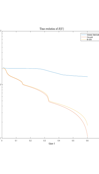
Figure 11: Allen-Cahn equation - Energy vs time - Comparison between globally stabilized one grid method, one grid method and high mode stabilized bi-grid method, $\epsilon=0.03$, $\Delta t=7\times 10^{-3}$, $\tau=S/\epsilon^{2}$, $S=2$ (left), $S=2$ (right), $u_{0}(x,y)=\cos(4\pi x)\cos(4\pi y)$

4.4.2 High mode stabilization via a proper linearization for the nonlinear term (Scheme 4.2)

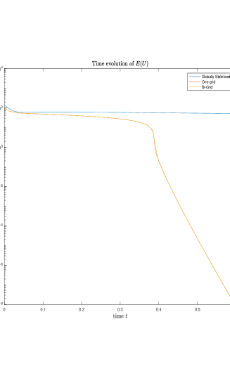
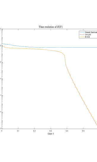
Figure 12: Allen-Cahn equation - Energy vs time - Comparison between globally stabilized one grid method, one grid method and bi-grid method. $\epsilon=0.03$, $\Delta t=7\times 10^{-3}$, $\tau=S/\epsilon^{2}$, $S=1.5$ (left), $S=10$ (right), $u_{0}(x,y)=\cos(\pi x)\cos(\pi y)$

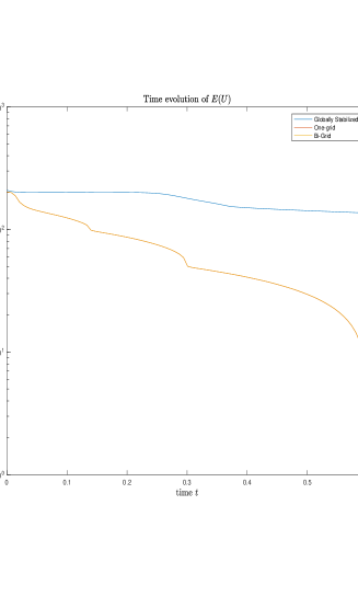
Figure 13: Allen-Cahn equation - Energy vs time - Comparison between Globally stabilized one grid method, one grid method and bi-grid method. $\epsilon=0.03$, $\Delta t=7\times 10^{-3}$. $\tau=S/\epsilon^{2}$, $S=1.5$ (left), $S=10$ (right). $u_{0}(x,y)=\cos(4\pi x)\cos(4\pi y)$

We have plotted for different initial data in Figures 12 and 13 the time evolution of the energy for the 3 methods. We observe that for same stabilization parameters, the bi-grid schemes based on high mode damping restitue an energy dynamics comparable to that of the reference scheme while the one-grid stabilization slows down the decreasing of the energy. Also, as expected, higher values of $\tau$ produces more important energy slow down for the stabilized one-grid scheme. Same results are obtained using $P_{1}$ elements instead of $P_{2}$.

Scheme	$\epsilon$	$S$	$\tau=S/\epsilon^{2}$	$\Delta t$	Stability
one-grid stab Scheme 2	$0.03$	$0.1$	$111.11$	$0.007$	yes
bigrid Scheme 3	$0.03$	$0.1$	$111.11$	$0.007$	yes
one-grid stab Scheme 2	$0.03$	$0.05$	$55.55$	$0.007$	no
bigrid Scheme 3	$0.03$	$0.05$	$55.55$	$0.007$	yes
one-grid stab Scheme 2	$0.03$	$0.01$	$1.11$	$0.007$	no
bigrid Scheme 3	$0.03$	$0.01$	$11.11$	$0.007$	yes

Table 1: $\epsilon=0.03,\ \Delta t=0.007,\ u_{0}(x,y)=\cos(4\pi x)\cos(4\pi y)$, $P_{2}$ elements

Scheme	$\epsilon$	$S$	$\tau=S/\epsilon^{2}$	$\Delta t$	Stability
one-grid stab Scheme 2	$0.03$	$10$	$111111.11$	$0.01$	yes
bigrid Scheme 3	$0.03$	$10$	$111111.11$	$0.01$	yes

Table 2: $\epsilon=0.03,\ \Delta t=0.01,\ u_{0}(x,y)=\cos(4\pi x)\cos(4\pi y)$, $P_{1}$ elements

Scheme	$\epsilon$	$S$	$\tau=S/\epsilon^{2}$	$\Delta t$	Stability
one-grid stab Scheme 2	$0.03$	$0.1$	$111.11$	$0.007$	no
bigrid Scheme 3	$0.03$	$0.1$	$111.11$	$0.007$	no

Table 3: $\epsilon=0.03,\ \Delta t=0.01,\ u_{0}(x,y)=\cos(8\pi x)\cos(7\pi y)$, $P_{2}$ elements

We finish with two illustrations obtained in the case in which the same triangulation is used for the two FEM spaces $W_{H}$ and $V_{h}$ is used. We choose

$$W_{H}=\{v_{H}\in{\cal C}^{0}({\bar{\Omega}})/v_{H}|_{K}\in P_{1},\ \forall K\in{\cal T}_{h}\}\mbox{ and }V_{h}=\{v_{h}\in{\cal C}^{0}({\bar{\Omega}})/v_{h}|_{K}\in P_{2},\ \forall K\in{\cal T}_{h}\}.$$

We have $W_{H}\subset V_{h}$. We first consider the Allen-Cahn equation on the torus $\Omega=\{(x,y)\in R^{2}/1\leq x^{2}+y^{2}\leq 9\}$. The dimensions are $\mbox{dim}(V_{h})=1606$, $\mbox{dim}(W_{H})=424$, $DR(W_{H},V_{h})=0.26401$.
The time evolution of the energy for the three methods is reported on Figure 14 (left); the conclusions are the same as in the previous examples: the high mode stabilization allows to stabilize without deteriorating the dynamics. We also consider $\Omega=]0,1[^{2}$ and $\mbox{dim}(V_{h})=14641$, $\mbox{dim}(W_{H})=3721$, $DR(W_{H},V_{h})=0.254149$. The time evolution of the energy is related on Figure (14) (right).

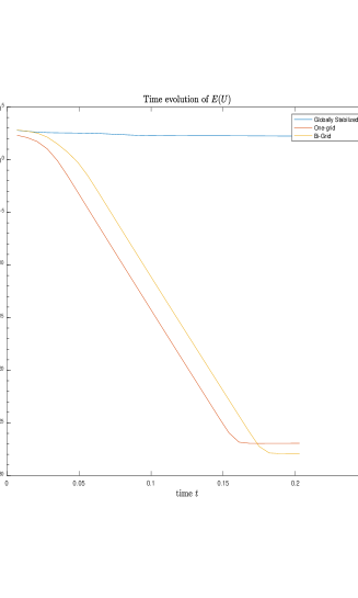
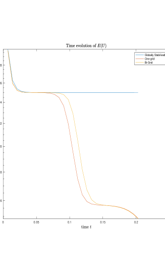
Figure 14: (left) $\Omega$ is the torus (R=1, R=3)- Energy vs time - Comparison between Globally stabilized one grid method, one grid method and high mode stabilized bi-grid method with linearization. $\epsilon=0.1$, $\Delta t=7\times 10^{-3}$. $\tau=S/\epsilon^{2}$, $S=0.01$ (left), $S=2$ (right). $u_{0}(x,y)=cos((x^{2}+y^{2}-1)*(x^{2}+y^{2}-9))^{2}$. (right) $\Omega$ is the unit square- Energy vs time - Comparison between Globally stabilized one grid method, one grid method and high mode stabilized bi-grid method with linearization. $\epsilon=0.1,\Delta t=7\times 10^{-3},\tau=S/\epsilon^{2},S=0.1,u_{0}(x,y)=\cos(4\pi x)\cos(4\pi y)$, $P_{1}$ elements on $W_{H}$, $P_{2}$ on $V_{h}$

4.4.3 Direct Simulation

Here $\Omega=]0,1[^{2}$ and two triangulations ${\cal T}_{h}$ and ${\cal T}_{H}$ are considered; they are composed of 1681 and 441 triangles respectively. The dimensions of the FEM spaces are $\mbox{dim}(W_{H})=1681$ and $\mbox{dim}(V_{h})=6561$, so $DR(W_{H},V_{h})=0.256211$.
To illustrate the robustness of the bi-grid method (Scheme 4.2), we make comparison with the one grid unconditionally stable scheme (Scheme 2). We observe that time history of the energy is comparable and that the time-evolution of the difference between the solutions produced by these schemes remains small. Finally, we observe that the CPU time is reduced for the bi-grid scheme, by a factor larger than 4.

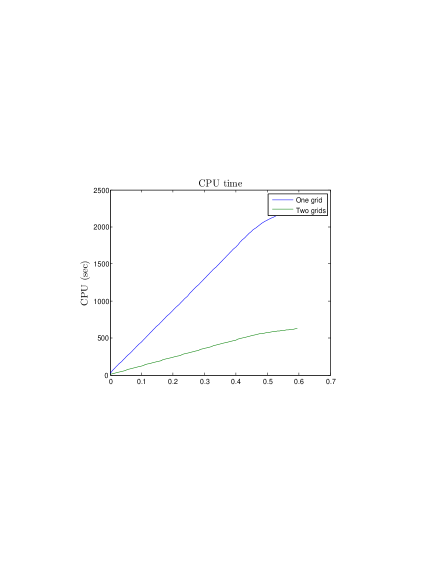
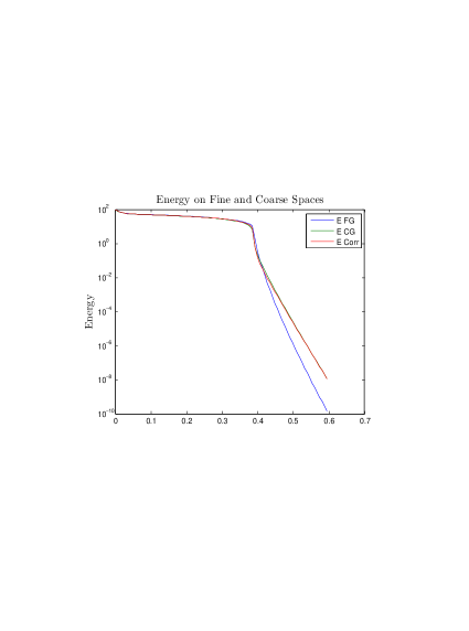
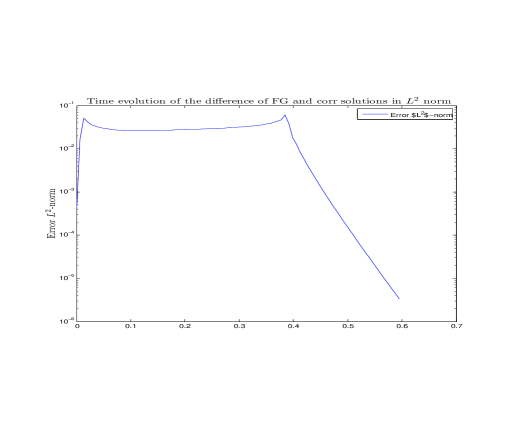
Figure 15: Allen-Cahn equation $\epsilon=0.03,\tau=5\times 10^{-3}$ and $\Delta t=7\times 10^{-3}$.

4.4.4 Simulation of an exact solution

We here always consider $\Omega=]0,1[^{2}$ two triangulations ${\cal T}_{h}$ and ${\cal T}_{H}$ composed of 1681 and 441 triangles respectively. The dimensions of the FEM spaces are $\mbox{dim}(W_{H})=1681$ and $\mbox{dim}(V_{h})=6561$, so $DR(W_{H},V_{h})=0.256211$. We now compare the bi-grid method (Scheme 4.2) and the one-grid Scheme 2 simulating an exact solution: we choose the function $u_{ex}(x,y,t)=\cos(\pi x)\cos(\pi y)exp(\sin(\pi t))$ to be the solution, an appropriate r.h.s. is added to this aim. As above, we observe that the error is small while the CPU time is reduced by a factor 3 in Figure (16), for $\epsilon=0.5$), and larger than 4 in Figure (17), for $\epsilon=0.3$.

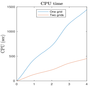
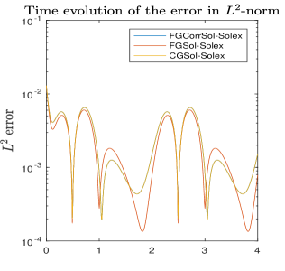
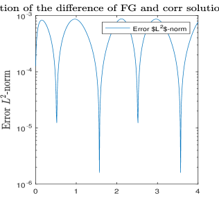
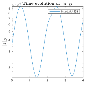
Figure 16: Allen-Cahn - simulation of an exact solution $\epsilon=0.5,\tau=12$, $\Delta t=10^{-2}$.

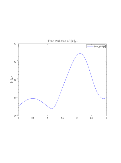
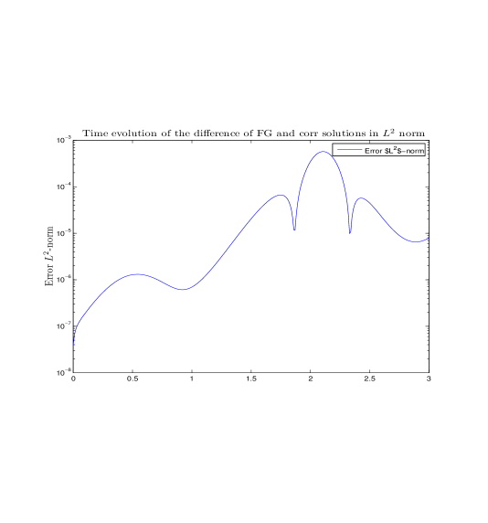
Figure 17: Allen-Cahn - simulation of an exact solution $\epsilon=0.3,\tau=1.8$, $\Delta t=10^{-2}$.

5 Concluding Remarks

The two-grid method in Finite Elements for reaction-diffusion equations we have presented here allows to produce fast and stable iterations, we gave also numerical evidences that our schemes capture important properties such as energy diminishing, which is fundamental when considering gradient flow models . This can be extended to a larger number of nested spaces, such as in [14, 15, 22], hoping to save much more computing time.
The separation of the scale allows to damp mainly the high mode components of the solution, this procedure can be interpreted as high-mode smoother.
An important advantage of the bi-grid framework is that it is not needed to work with embedded spaces, particularly it is not necessary to compute a hierarchical-like basis, the filtering is automatically provided by the prolongation step. We have considered here first reaction-diffusion problems: it is a first study to be done and to be validated before applying the method to more complex systems.

References

- [1] H. Abboud, V. Girault, T. Sayah. A second order accuracy for a full discretized time-dependent Navier-Stokes equations by a two-grid scheme. Numer. Math. DOI 10. 1007/s00211-009-0251-5.
- [2] M. Abounouh, H. Al Moatassime, J-P. Chehab, S. Dumont, O. Goubet. Discrete Schrodinger equations and dissipative dynamical systems. Communications on Pure and Applied Analysis, 7 (2008), no 2, 211-227.
- [3] S. M. Allen, J. W. Cahn. A microscopic theory for antiphase boundary mo- tion and its application to antiphase domain coarsening. Acta Metall. Mater., 27:10851095, 1979.
- [4] S. M. Allen, J. W. Cahn. Ground State Structures in Ordered Binary Alloys with Second Neighbor Interactions. Acta Met. 20, 423 (1972).
- [5] S. M. Allen, J. W. Cahn. A Correction to the Ground State of FCC Binary Ordered Alloys with First and Second Neighbor Pairwise Interactions. Scripta Met. 7, 1261 (1973).
- [6] R. E. Bank Hierarchical Bases and the Finite Element. Acta Numerica (1996), pp. 1–43.
- [7] R. E. Bank, J. Xu. An Algorithm for Coarsening Unstructured Meshes. Numerische Mathematik 73 (1996), 1–36.
- [8] S. Bartels. Numerical Methods for Nonlinear Partial Differential Equations. Springer Series in Computational Mathematics 47, 015
- [9] C. Brezinski, J.-P. Chehab. Nonlinear hybrid procedures and fixed point iterations. Num. Funct. Anal. Opti. 19 (1998), 465-487.
- [10] M. Brachet, J.-P. Chehab. Stabilized Times Schemes for High Accurate Finite Differences Solutions of Nonlinear Parabolic Equations. Journal of Scientific Computing, 69 (3), 946-982, 2016
- [11] J.-P. Chehab, B. Costa. Multiparameter schemes for evolutive PDEs. Numerical Algorithms, 34 (2003), 245-257.
- [12] J.-P. Chehab, B. Costa. Time explicit schemes and spatial finite differences splittings. Journal of Scientific Computing, 20, 2 (2004), pp 159-189.
- [13] B. Costa, L. Dettori, D. Gottlieb, R. Temam. Time marching techniques for the nonlinear Galerkin method. SIAM J. SC. comp., 23, (2001), 1, 46–65.
- [14] T. Dubois, F. Jauberteau, R. Temam. Dynamic Multilevel Methods and the Numerical Simulation of Turbulence. Cambridge University Press (1998)
- [15] T. Dubois, F. Jauberteau, R. Temam. Incremental Unknowns, Multilevel Methods and the Numerical Simulation of Turbulence. Comp. Meth. in Appl. Mech. and Engrg. (CMAME), Elsevier Science Publishers (North-Holland).
- [16] C. M. Elliott. The Cahn-Hilliard Model for the Kinetics of Phase Separation. Mathematical Models for Phase Change Problems, International Series of Numerical Mathematics, Vol. 88,(1989) Birkhäuser.
- [17] C. M. Elliott, A. Stuart The global dynamics of discrete semilinear parabolic equations. SIAM J. Numer. Anal. 30 (1993) 1622–1663.
- [18] H. Emmerich. The Diffuse Interface Approach in Materials Science Thermodynamic. Concepts and Applications of Phase-Field Models. Lecture Notes in Physics Monographs, Springer, Heidelberg, 2003.
- [19] A. Ern, J.-L. Guermond. Theory and Practice of Finite Elements. Applied Mathematical Science, 159, Springer-Verlag, New-York, 2004.
- [20] D. J. Eyre. Unconditionallly Stable One-step Scheme for Gradient Systems. June 1998, unpublished, http://www.math.utah.edu/eyre/research/methods/stable.ps.
- [21] FreeFem++ page. http://www.freefem.org
- [22] Y. He, K-M. Liu, W. Sun. Multi-level spectral galerkin method for the navier-stokes problem I : spatial discretization. Numer. Math. (2005) 101: 501—522
- [23] J. Jiang, J. Shi. Bistability Dynamics in Structured Ecological Models. Spatial Ecology, Stephen Cantrell, Chris Cosner, Shigui Ruan ed., CRC Press, 2009
- [24] C. Lemaréchal, Une méthode de résolution de certains systèmes non linéaires bien posés, C.R. Acad. Sci. Paris, sér. A, 272 (1971), 605–607.
- [25] Y. Li, D. Jeong, J. Choi, S. Lee, J. Kim. Fast local image inpainting based on the Allen–Cahn model. Digital SignalProcessing37(2015), 65–74
- [26] M. Marion,J. Xu. Error estimates on a new nonlinear Galerkin method based on two-grid finite elements. SIAM J. Numer. Anal. 32 (1995), no. 4, 1170?1184.
- [27] B. Merlet, M. Pierre, Convergence to equilibrium for the backward Euler scheme and applications. Commun. Pure Appl. Anal. 9 (2010), no. 3, pp. 685–702.
- [28] J. Shen, X. Yang, Numerical Approximations of Allen-Cahn and Cahn-Hilliard Equations. DCDS, Series A, (28), (2010), pp 1669–1691.
- [29] J. Xu, Some Two-grids finite element methods. Contemporary Mathematics, vol 157, 1994.