Spatially variant PSF modeling in confocal macroscopy

Abstract.

Point spread function (PSF) plays an essential role in image reconstruction. In the context of confocal microscopy, optical performance degrades towards the edge of the field of view as astigmatism, coma and vignetting. Thus, one should expect the related artifacts to be even stronger in macroscopy, where the field of view is much larger. The field aberrations in macroscopy fluorescence imaging system was observed to be symmetrical and to increase with the distance from the center of the field of view. In this paper we propose an experiment and an optimization method for assessing the center of the field of view. The obtained results constitute a step towards reducing the number of parameters in macroscopy PSF model.

1. Introduction

The PSF determination is a crucial preliminary step to image restoration [13]. Even if one resorts to blind deconvolution schemes, a priori knowledge related to the PSF is desired [21], [4], [19]. This knowledge can be acquired by studying PSF theoretical properties. In the context of fluorescence imaging, the theoretical approach usually relies on diffraction-limited PSF model [11]. Experimental PSFs may be measured using calibration beads [24] or directly from the image by extracting small point-like objects [23]. Such PSFs can be used for instance to validate theoretical parametric PSF model or to assess the aberration of point spread function in given imaging systems [15]. The PSF modeling problem becomes more complex if the PSF is not spatially invariant. The space variation model usually relies on one of the following strategies. Firstly, assuming that the PSF variation is smooth, the PSF can be represented as a weighted sum of basis functions [2]. The efficiency can be further improved by applying interpolation methods [7]. Alternatively an image can be segmented into regions inside which PSFs are assumed to be invariant [17]. Recently in [20] the authors shown experimentally that the first strategy leads to the better results. While in this work the focus was on astronomical images, we will concentrate on macroscopy.

In high angular resolution images the PSF varies in the field of view, i.e. the optical aberrations increase towards the margins. This phenomena occurs in the context of astronomy [7], [20] (2D-PSF) or macroscopy [10], where the principal axis of the PSFs around each bead were observed to converge to one point, called here the optical center. In macroscopy the problem of field aberration is coupled with the problem of out-of-focus blur, in the depth-direction, due to the diffraction-limited nature of the lens. 3D-PSF model for confocal macroscopy was previously studied in [14]. One limitation of the proposed PSF model is that it requires two parameters to be estimated at each pixel position. Certainly, the problem is untraceable without any prior knowledge about unknown parameters. The second limitation of this previous work is that there is no analysis related to variation of field aberrations with depth (experimental data in this study were limited to beads mounted only on one depth). Indeed in fluorescence microscopy, the aberrations increase as a function of depth from the coverslip [1], [16, Chapter 23]. The experimental study presented in [10] indicate that the typical for confocal microscopy intensity decrease and effect of growing PSF size with depth are not present in macroscopy.

In this paper, we investigate the confocal macroscopy PSFs symmetry. We propose a procedure and experimental setup for optical center identification. Our main contribution lies in the problem formulation, its resolution and the evaluation of these results. The experimental results show that our proposed model and its solution fits the experimental data well.

The paper is organized as follows. We present two alternative problem formulation in Section 2. Next, in Section 3 the related optimization methods are discussed. The two models are compared on synthetic data in Section 4, which also illustrates the performance of our approaches on real data. Finally, Section 5 concludes the paper.

2. Problem statement

2.1. Notation

Let $\left(P_{i}\right)_{i\in\left\{1,\ldots,N\right\}}$ be a finite set of identified PSFs. Let $a=(a_{i})_{1\leq i\leq N}$ where for all $i\in\left\{1,\ldots,N\right\}$ $a_{i}\in\mathbb{R}^{K}$ is a center of mass of $P_{i}$, and $n_{i}\in\mathbb{R}^{K}$ the unit vector indicating the principal axis of inertia of $P_{i}$. Since we consider 3D images, in the following $K=3$. Let $c\in\mathbb{R}^{K}$ be a point. The distance from $c$ to the line $\{a_{i},n_{i}\}$ is given by:

$$\text{dist}(c,\{a_{i},n_{i}\})=\Phi(r_{i}-(r_{i}^{\top}n_{i})n_{i})$$ (1)

where $r_{i}\in\mathbb{R}^{K}$ is a vector from point $a_{i}$ to $c$ and $\Phi$ is some distance measure. More generally we will consider $\Phi$ to be any error measure in $\Gamma_{0}(\mathbb{R}^{K})$. Fig. 1 illustrates the case of $\Phi$ given by $\left\|\cdot\right\|$.

Figure 1. Distance from a point $c$ to a line $\{a_{i},n_{i}\}$ in arbitrary dimensions Euclidean space.

Thus we have

$$r_{i}-(r_{i}^{\top}n_{i})n_{i} =(c-a_{i})-(c-a_{i})^{\top}n_{i}n_{i}$$

$$=(I-n_{i}n_{i}^{\top})(c-a_{i})$$

$$=(I-n_{i}n_{i}^{\top})c-(I-n_{i}n_{i}^{\top})a_{i}$$ (2)

where $I$ is the $K\times K$ identity matrix. Using the introduced notation we formulate the problem of finding the coordinates of optical center denoted by $\widehat{c}\in\mathbb{R}^{K}$. Note that ideally, the distance from any line $\{a_{i},n_{i}\}$ to the optical center should be $0$. However, as the measurements are noisy, the problem of finding the optical center needs to be formulated in an optimization framework. The data include the measurements of $(a_{i})_{1\leq i\leq N}$ and $(n_{i})_{1\leq i\leq N}$. Next, the observation model of them is presented.

2.2. Observations model

Let, for all $i\in\left\{1,\ldots,N\right\}$, $\widetilde{a}_{i}\in\mathbb{R}^{K}$ and $\widetilde{n}_{i}\in\mathbb{R}^{K}$ be vectors of observations related to an original center of mass $a_{i}$ and the principal orientation $n_{i}$. Next we propose two formulations which relate the observations and optical center.

Model 1.

Let $x\in\mathcal{X}$ be a vector of unknown variables defined as $x=c$ and $\mathcal{X}=\mathbb{R}^{K}$. Let $H\in\mathcal{H}=\mathbb{R}^{K\times KN}$ be defined as $H=[H_{1},\ldots,H_{N}]^{\top}$, where $H_{i}\in\mathbb{R}^{K\times K}$ is given by $H_{i}=\omega_{i}\left(I-\widetilde{n}_{i}\widetilde{n}_{i}^{\top}\right)$. For all $i\in\left\{1,\ldots,N\right\}$ $\omega_{i}$ denotes a positive weight. Let $y\in\mathcal{Y}$ be a vector of observations with $\mathcal{Y}=\mathbb{R}^{KN}$. We define $y$ as $y=(y_{i})_{1\leq i\leq N}$ where for all $i\in\left\{1,\ldots,N\right\}$ $y_{i}\in\mathbb{R}^{K}$ is a weighted vector of observations such that $y_{i}=H_{i}\widetilde{a}_{i}$. Hence from (2) we obtain the following model

$$y=(H+\Delta H)x+\Delta y$$ (3)

where $\Delta H\in\mathcal{H}$ and $\Delta y\in\mathcal{Y}$ are some error, resulting from uncertainty of measurements on $H$ and $y$, respectively.

Introducing the variable $d_{i}\in\mathbb{R}$, defined for all $i\in\left\{1,\ldots,N\right\}$ as $d_{i}=n_{i}^{\top}(c-a_{i})$ transforms (2) into a linear functional in terms of $n_{i}$, $a_{i}$ and $c$, i.e.

$$r_{i}-(r_{i}^{\top}n_{i})n_{i} =c-a_{i}-n_{i}d_{i}.$$ (4)

The variable $d_{i}$ can be regarded as the length of the line segment connecting $a_{i}$ and the point given by projection of $c$ on the line $\{a_{i},n_{i}\}$. The collections of variable $(d_{i})_{1\leq i\leq N}$ forms vector $d$. Using this change of variables, we develop the following formulation.

Model 2.

Let $y\in\mathcal{Y}=\mathbb{R}^{KN}$ be a vector of observations defined as $y=(\omega_{i}a_{i})_{1\leq i\leq N}$. The related vector of unknown variables $x\in\mathcal{X}=\mathbb{R}^{N+K}$ is given by $x=[c,d]^{\top}$. Let $H\in\mathcal{H}=\mathbb{R}^{NK\times(K+N)}$ be defined as $H=\left[\mathsf{C}\;\mathsf{D}\right]$, where $\mathsf{C}=\left(\omega_{i}\;I\right)_{1\leq i\leq N}$ and $\mathsf{D}=\left(\mathsf{D}^{\left(i,j\right)}\right)_{1\leq i\leq N,1\leq j\leq N}$ with non zero elements $\mathsf{D}^{\left((i-1)K+j,i\right)}=\omega_{i}n_{i}^{(j)}$. Using introduced notations, from (4), we obtain the following model

$$y=(H+\Delta H)x+\Delta y$$ (5)

where $\Delta H\in\mathcal{H}$ and $\Delta y\in\mathcal{Y}$ are some error, resulting from uncertainty of measurements on $n_{i}$ and $a_{i}$, respectively.

The advantage of the first formulation over the second one is the reduced size of unknown vector $x$. Especially that usually the number of observations $N$ is much greater than the dimensionality of search space $K$, i.e. $N\gg K$. However the first formulation may lead to complex statistical properties of errors $\Delta H$ and $\Delta x$, which can be regarded as drawback. In Formulation 2, an auxiliary variable $d$ is introduced, which depends on the variable $c$, whereas this dependence is not taken into account explicitly. This should lead to a suboptimal results. However, an interesting observation is that for $\Phi=\left\|\cdot\right\|$, we obtain as an optimal solution to the problem $\operatorname{argmin}_{c,d}\sum_{i=1}^{N}\left\|c-a_{i}-d_{i}n_{i}\right\|$, $\forall i\in\left\{1,\ldots,N\right\}\;d_{i}=c-a_{i}^{\top}n_{i}$. Hence in such case the relation is given implicitly. For another choices of $\Phi$ the problem remains open. One method to account for outliers in both formulations is to set appropriately $\omega_{i}$. An interesting choice for $\omega_{i}$ could be the ratio between the first and second eigenvalue provided by PCA.

2.3. Problem

Next we formulate an optimization problem. The goal is to find an estimate $\widehat{x}$. and from this solution to recover the desired estimate of the optical center $\widehat{c}$.

Problem 1.

Let $\left(\psi_{r}\right)_{1\leq r\leq R}:\mathbb{R}^{P_{r}}\mapsto\mathbb{R}$ be functions in $\Gamma_{0}(\mathbb{R}^{P_{r}})$. We want to:

$$\underset{\begin{subarray}{c}{x\in\mathcal{X}}\end{subarray}}{\mathrm{minimize}}\;\;\Phi\big{(}Hx-y\big{)}+\iota_{C}(x)+\sum_{r=1}^{R}\psi_{r}(V_{r}x).$$ (6)

where $\iota_{C}$ is an indicator function of $C$ and $C$ is a closed convex subset of $\mathcal{X}$.

The hereabove problem admits the following interpretation. We seek a point $\widehat{c}$ minimizing (6), i.e. the distance between this point and the line stemming from all measured PSFs and oriented along all the main axes of inertia, subject to some constraints. The measurement of the center of mass $a_{i}$ are assumed to be noisy.

Problem 2.

We want to:

$$\underset{\begin{subarray}{c}{\begin{subarray}{c}x\in\mathcal{X},\;\Delta y\in\mathcal{Y},\\ \Delta H\in\mathcal{H}\end{subarray}}\end{subarray}}{\mathrm{minimize}}\;\; \left\|\Delta y\right\|^{2}+\left\|\Delta H\right\|^{2}\;\;\text{such that}\;\;$$

$$\quad\quad(H+\Delta H)x-(y+\Delta y)=0$$ (7)

where $\Delta b$ and $\Delta h$ model the perturbations on $b$ and $h$, respectively. One can recover from the solution $\widehat{z}$ of the above problem, the desired estimate of the optical center $\widehat{x}$.

The objective of this work is to address the Problem 1 and the Problem 2. Note that the second problem formulation is more realistic, due to the assumption that both measurements, $a_{i}$ and $n_{i}$, are subject to noise. However, Problem 1 allows for appropriate choice of $\Phi$ that can handle outliers.

3. Optimization framework

In some special case, the solution of the Problem 1 admits the closed form expression. For instance, in case of Formulation 1, $C=\mathcal{X}$, $R=0$ and $\Phi(u)=\sum_{i=1}^{N}\left\|u_{i}\right\|^{2}$ we have:

$$\widehat{x}=\left(\sum_{i=1}^{N}H_{i}^{\top}H_{i}\right)^{-1}\left(\sum_{i=1}^{N}H_{i}^{\top}y_{i}\right)$$ (8)

So we just need to inverse $K\times K$ matrix. More generally, the more robust choices of $\Phi$ can be considered. Interesting cases could be: $\Phi(u)=\|u\|_{1}$, $\Phi(u)=\|u\|$, $\Phi(u)=\sum_{i=1}^{N}\|u_{i}\|$, $\Phi(u)=L_{t}(\|u\|)$, $\Phi(u)=\sum_{i=1}^{N}L_{t}\left(\|u_{i}\|\right)$, where $L_{t}$ denotes Huber function, i.e.

$$L_{t}(u)=\begin{cases}\frac{1}{2}u^{2}&\text{if}\left|u\right|\leq t\\ t\left(\left|u\right|-0.5t\right)&\text{otherwise}\end{cases}$$ (9)

In such cases, one can resort to proximal splitting algorithms. One possibility is to use the primal-dual algorithm [6] summarized in Algorithm 1.

Algorithm 1 Primal-dual algorithm for solving (6).

  Initialization:

  Set $x_{0}\in\mathbb{R}^{K}$, and $(\forall r\in\left\{0,\ldots,R\right\})$ $v_{r,0}\in\mathbb{R}^{P_{r}}$.

  Iterations:

  For $k=0,\ldots$

  $\left\lfloor\begin{array}[]{l}y_{1,k}=x_{k}-\gamma\left(H^{\top}v_{0,k}+\sum_{r=1}^{R}V_{r}^{\top}v_{r,k}\right)\\ p_{1,k}=\operatorname{prox}_{\gamma\iota_{C}}(y_{1,k})\\ y_{2,0,k}=v_{0,k}+\gamma Hx_{k}\\ p_{2,0,k}=y_{2,0,k}-\gamma\left(\operatorname{prox}_{\gamma^{-1}\Phi}(\gamma^{-1}y_{2,0,k}-y)+y\right)\\ q_{2,0,k}=p_{2,0,k}+\gamma Hp_{1,k}\\ v_{0,k+1}=v_{0,k}-y_{2,0,k}+q_{2,0,k}\\ \mbox{For}\;r=1,\ldots,R\\ \left\lfloor\begin{array}[]{l}y_{2,r,k}=v_{r,k}+\gamma V_{r}x_{k}\\ p_{2,r,k}=y_{2,r,k}-\gamma\operatorname{prox}_{\gamma^{-1}\psi_{r}}(\gamma^{-1}y_{2,r,k})\\ q_{2,r,k}=p_{2,r,k}+\gamma V_{r}p_{1,k}\\ v_{r,k+1}=v_{r,k}-y_{2,r,k}+q_{2,r,k}\end{array}\right.\\ q_{1,k}=p_{1,k}-\gamma\left(H^{\top}p_{2,0,k}+\sum_{r=1}^{R}V_{r}^{\top}p_{2,r,k}\right)\\ x_{k+1}=x_{k}-y_{1,k}+q_{1,k}\\ \end{array}\right.$

It is worth noticing that the proximity operators of the functions of interest are given explicitly, i.e.:

$$\operatorname{prox}_{\gamma\left|\cdot\right|}(x)=\begin{cases}\left(\left|x\right|-\gamma\right)\odot\text{sign}(x)&\text{if}\quad\left|x\right|\geq\gamma\\ 0&\text{otherwise}\end{cases}$$ (10)

$$\operatorname{prox}_{\gamma\left\|\cdot\right\|}(x)=\begin{cases}x\left(1-\frac{\gamma}{\left\|x\right\|}\right)&\text{if}\quad 1-\frac{\gamma}{\left\|x\right\|}>0\\ 0&\text{otherwise}\end{cases}$$ (11)

$$\operatorname{prox}_{\gamma L_{t}(x)}=\begin{cases}\frac{x}{\gamma+1}&\text{if}\quad\left|x\right|\leq\frac{t}{\sqrt{\gamma}}(\gamma+1)\\ x-t\sqrt{\gamma}\;\text{sign}(x)&\text{otherwise}\end{cases}$$ (12)

Moreover we recall from [5] that proximity operator $p=\operatorname{prox}_{\gamma\Phi}(u)$ where $\Phi=\sum_{i}\Phi_{i}(u_{i})$ is equal to $p=[p_{1}^{\top},...,p_{N}^{\top}]^{\top}$, where $p_{i}=\operatorname{prox}_{\gamma\Phi_{i}}(u_{i})$. The Problem 2 can be efficiently addressed using total least square (TLS) approach [9], [12].

4. Simulations

4.1. Synthetic data

Here we report experimental results to the Problems 1 and  2 using methods described in the previous section. The study aims at testing the performance of two approaches under the conditions simulating the experiment with images of point sources (beads) mounted on different depth. Since we consider three dimensional macroconfocal images, in all our experiments $K$ is set to $3$. We evaluate the performance of our approaches using $200$ randomly generated center of mass of $P_{i}$ distributed at $2$ layers. For all $i\in\left\{0,\ldots,N\right\}$ coordinates $a_{i}^{(1)}$ and $a_{i}^{(2)}$ are uniformly distributed over $\left[0,2048\right]$ while coordinate $a_{i}^{(3)}$ take value from set $\left\{50,250\right\}$. The original optical center position $\overline{c}=\left[1000,1000,5000\right]^{\top}$.

For all $i\in\left\{1,\ldots,N\right\}$ $\widetilde{a}_{i}$ and $\widetilde{n}_{i}$ are related to an original center of mass $a_{i}$ and the principal orientation $n_{i}$ through the Bernoulli-Gaussian model of the following form

$$\widetilde{n}_{i}=n_{i}+\epsilon_{i}u_{i}+(1-\epsilon_{i})w_{i},$$ (13)

$$\widetilde{a}_{i}=a_{i}+\epsilon_{i}s_{i}+(1-\epsilon_{i})t_{i},$$ (14)

where $\epsilon_{i}$ is a binary variable and $w_{i}=\left(w_{i}^{(j)}\right)_{1\leq j\leq K}$, $u_{i}=\left(u_{i}^{(j)}\right)_{1\leq j\leq K}$, $s_{i}=\left(s_{i}^{(j)}\right)_{1\leq j\leq K}$, $t_{i}=\left(t_{i}^{(j)}\right)_{1\leq j\leq K}$ are realizations of normally distributed random variable $W_{i}$, $U_{i}$, $S_{i}$, $T_{i}$, respectively, such that:

$$\begin{array}[]{ c c}U_{i}^{(j)}\sim\mathcal{N}(0,\sigma^{2}_{1})&\quad W_{i}^{(j)}\sim\mathcal{N}(0,\sigma^{2}_{2})\\ S_{i}^{(j)}\sim\mathcal{N}(0,\sigma^{2}_{3})&\quad T_{i}^{(j)}\sim\mathcal{N}(0,\sigma^{2}_{4})\end{array}$$ (17)

The binary variable $\epsilon_{i}$ takes value according to the following rule:

$$\epsilon_{i}=\begin{cases}0&\text{if}\;\rho_{i}\leq\varepsilon\\ 1&\text{otherwise}\end{cases}$$ (18)

$\rho_{i}$ is an random variable uniformly distributed in $[0,1]$ and $\varepsilon$ denotes the probability of occurrence of outliers. Thus, $\sigma_{1}$, $\sigma_{3}$ and $\sigma_{2}$, $\sigma_{4}$ denote standard deviation of inliers and outliers, respectively. Consequently, we have $\sigma_{2}>\sigma_{1}$ and $\sigma_{4}>\sigma_{3}$. The results for $\varepsilon=0.25$, $\sigma_{1}=0.015$, $\sigma_{2}=0.030$, $\sigma_{3}=30$, $\sigma_{4}=60$ are summarized in Tables 2 and  2. We provide for all $j=\left\{1,\ldots,K\right\}$ the estimate bias and variance of $\widehat{c}$ averaged over $100$ noise realizations and normalized over true $\overline{c}^{(j)}$. The results include also mean squared error (MSE) averaged over $100$ noise realizations.

		Formulation 1			Formulation 2
	$\Phi(u)$	$\|u\|_{1}$	$\|u\|$	$\L_{t}(u)$	$\|u\|_{1}$	$\|u\|$	$\L_{t}(u)$
		Bias ($\%$)
j	1	-0.03	-0.13	-0.02	0.03	-0.03	0.02
	2	-0.30	-0.30	-0.29	-0.18	-0.14	-0.19
	3	4.50	7.30	4.42	2.46	2.47	2.39
		Sigma ($\%$)
j	1	0.77	0.72	0.75	0.69	0.67	0.69
	2	0.89	0.78	0.86	0.83	0.72	0.81
	3	4.58	7.37	4.51	2.58	2.59	2.51
MSE		225	365	221	123	124	120

Table 1. Optical center estimation problem results (Problem 1)

		Formulation 1	Formulation 2
		Bias ($\%$)
j	1	-0.21	0.02
	2	-0.30	-0.06
	3	0.53	-0.08
		Sigma ($\%$)
j	1	0.69	0.66
	2	0.78	0.73
	3	0.92	0.77
MSE		40	34

Table 2. Optical center estimation problem results (Problem 2)

One can observe that the Problem formulation given in 2 applied to Formulation 2 leads to the best results, i.e. the obtained results are almost unbiased and the standard deviation of estimate is lower than $1\%$. Hence, we choose this approach to be confronted with a challenge originating from real data.

4.2. Real data

To assess experimentally the PSF depth variation we use the experimental described in [10, Fig. 8.2]. In the experimental sample, the beads were distributed over two layers. Images were acquired using a macro confocal laser scanning microscope (Leica TCS-LSI). Measurements were done on images taken according to the following settings: pinhole $1.0$ airy, $400$ Hz scan speed, excitation line $405/532$ nm, and emission range $534$ nm-$690$nm.

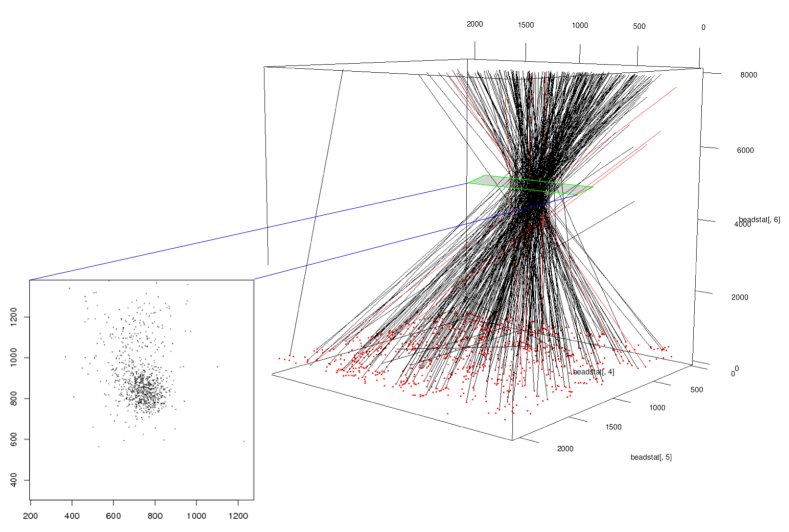
Figure 2. An example illustrating PSFs cone

As a pre-processing step, we propose to segment all the PSF in the acquired image and then to detect their center and their principal axis. The following procedure is proposed: (1) Find the discrete finite set of ellipsoids in an image, which we assume to be related by injection with PSFs. (2) Compute the grey-level statistics of each independent ellipsoid. The difficulties that can arise in the process of identifying the signal of interest associated with PSF stem from noise, beads sticking together in the original sample or very low image SNR. To overcome them, the following simple implementation using morphological tools is proposed. First, the noise is reduced by anisotropic Gaussian blurring. Then small maxima are suppressed by volume opening [22], which has the effect of suppressing small objects. A top-hat operator is then used to remove low frequency variations in the background [18]. Next, segmentation is performed by thresholding, resulting in a binary image where $1$ correspond to the signal of interest and $0$ the background. Finally we extend the volume of each detected nonzero ellipsoid using the Watershed algorithm [3], i.e. we search for the maximum region around each volume under the constraint that the regions of any two PSFs may not intersect. The size of resulting volume is also limited by maximum length, width and height. In the second step we compute the grey-level statistics of each independent ellipsoid. More specifically we use principal component analysis [8] to find the center and principal axis of each ellipsoid. An example of the results of the above described procedure is illustrated in Fig. 2. In the processed $12$ bit precision image stack of size $2048\times 2048\times 350$ we have identified $967$ PSFs, within $930$ lay in the first layer and only $37$ in the second one. As expected the results indicates that the collection of lines associated with couples (the PSF center, principal axis of the PSF) form a cone like shape. The cross-section over the PSFs cone in the the $x,y$ plane close to the optical center is illustrated in the zoomed image in Fig. 2. Ideally, one should expect only a point in this plane.

Figure 3. Deviation from the vertical in radians as a function of distance to the optical axis.

Next we identify the optical center using 2 applied to Formulation 2. For $\omega_{i}$ set to ratio between first and second eigenvalue we obtain $\widehat{c}=[688,887,5201]^{\top}$. Fig. 3 illustrates $\arccos(\widetilde{n}_{i}^{(3)})$ in a function of $\ell_{2}$ distance from $[\widetilde{a}_{i}^{(1)},\widetilde{a}_{i}^{(2)}]^{\top}$ to $[\widehat{c}^{(1)},\widehat{c}^{(2)}]^{\top}$ for beads whose ration between the first two eigenvalues are greater than $2.2$. The main orientation of PSF of the bead is well correlated to the distance from the bead to the optical axis. The relation is close to linear. This observation is consistent with radial symmetry of the PSFs, i.e with our main hypothesis, that all main PSF’s axis converge to one point. We note that the beads furthest away from the optical axis have an orientation of nearly $0.35$ radian, i.e. almost $20^{\circ}$.

5. Conclusions

In this paper we have presented an experimental study based on images of fluorescent bead which aim to find out if we could detect the position of the optical center towards which beads normally point. We have shown the position of the optical center to be estimated robustly in spite of this noise and despite the presence of noticeable outliers. We have observed that the PSFs orientation is consistent with radial invariance. The complexity of the problem has been reduced by applying several simplification, related to elliptic shape of PSF and noise distribution corrupting the identified PSFs center and main directions. This assumption may be relaxed provided that more experimental data are available.

References

- [1] F. Aguet, D. Van De Ville, and M. Unser. An accurate PSF model with few parameters for axially shift-variant deconvolution. pages 157–160. IEEE, 2008.
- [2] M. Arigovindan, J. Shaevitz, J. McGowan, J. W. Sedat, and D. A. Agard. A parallel product-convolution approach for representing the depth varying Point Spread Functions in 3D widefield microscopy based on principalcomponent analysis. Opt. Express, 18(7):6461–6476, Mar 2010.
- [3] S. Beucher and C. Lantuéjoul. Use of watersheds in contour detection. In Int. Workshop on Image Processing, Rennes, France, Sep. 1979. CCETT/IRISA.
- [4] J. Bolte, P. L. Combettes, and J.-C. Pesquet. Alternating proximal algorithm for blind image recovery. pages 1673–1676. IEEE, 2010.
- [5] P. L. Combettes and J.-C. Pesquet. Proximal splitting methods in signal processing. In H. H. Bauschke, R. S. Burachik, P.L. Combettes, V. Elser, D. R. Luke, and H. Wolkowicz, editors, Fixed-Point Algorithms for Inverse Problems in Science and Engineering, Springer Optimization and Its Applications, pages 185–212. Springer New York, 2011.
- [6] P. L. Combettes and J.-C. Pesquet. Primal-dual splitting algorithm for solving inclusions with mixtures of composite, Lipschitzian, and parallel-sum type monotone operators. Set-Valued and Variational Analysis, 20:307–330, 2012. 10.1007/s11228-011-0191-y.
- [7] L. Denis, E. Thiébaut, and F. Soulez. Fast model of space-variant blurring and its application to deconvolution in astronomy. pages 2817–2820. IEEE, 2011.
- [8] C. Eckart and G. Young. The approximation of one by another of lower rank. Psychometrika, 1(3):211–218, Sep. 1936.
- [9] G. H. Golub and C. F. Van Loan. An analysis of the total least squares problem. SIAM Journal on Numerical Analysis, 17(6):883–893, Dec. 1980.
- [10] A. Jezierska. Image Restoration in the presence of Poisson-Gaussian noise. PhD thesis, LIGM - Laboratoire d’Informatique Gaspard-Monge, 2013.
- [11] H. Kirshner, F. Aguet, D. Sage, and M. Unser. Least-square PSF fitting for localization microscopy. In Second Swiss Single Molecule Localization Microscopy Symposium (SSMLMS’12), Lausanne VD, Switzerland, Aug. 2012.
- [12] I. Markovsky and S. Van Huffel. Overview of total least-squares methods. 87(10):2283–2302, Oct. 2007.
- [13] J. G. McNally, T. Karpova, J. Cooper, and J. A. Conchello. Three-dimensional imaging by deconvolution microscopy. Methods, 19(3):373 – 385, 1999.
- [14] P. Pankajakshan, Z. Kam, A. Dieterlen, G. Engler, L. Blanc-Féraud, J. Zerubia, and J. C. Olivo-Marin. Point-spread function model for fluorescence MACROscopy imaging. pages 1364–1368, Chicago, USA, Nov. 2010.
- [15] P. Pankajakshan, Z. Kam, A. Dieterlen, and J.-C. Olivo-Marin. Characterizing the 3-D field distortions in low numerical aperture fluorescence zooming microscope. Optics Express, 20(9):9876–9889, 2012.
- [16] J. Pawley. Handbook of Biological Confocal Microscopy. Language of science. Springer, 2006.
- [17] M. Reràbek and P. Pàta. The space variant PSF for deconvolution of wide-field astronomical images. Acta Polytechnica, 48(3):79–83, 2008.
- [18] J. Serra. Image analysis and mathematical morphology. Academic Press, 1982.
- [19] F. Soulez, L. Denis, Y. Tourneur, and E. Thièbaut. Blind deconvolution of 3D data in wide field fluorescence microscopy. pages 1735–1738. IEEE, 2012.
- [20] E. Thi baut, L. Denis, F. Soulez, and R. Mourya. Spatially variant psf modeling and image deblurring. In Proc. SPIE, volume 9909, pages 99097N–99097N–10, 2016.
- [21] E. Thiébaut. Optimization issues in blind deconvolution algorithms. Astronomical Data Analysis II, 4847:174–183, 2002.
- [22] L. Vincent. Grayscale area openings and closings, their efficient implementation and applications. In Proceedings of the conference on mathematical morphology and its applications to signal processing, pages 22–27, Barcelona, Spain, May 1993.
- [23] M. Von Tiedemann, A. Fridberger, M. Ulfendahl, and J. Boutet De Monvel. Image adaptive point-spread function estimation and deconvolution for in vivo confocal microscopy. Microscopy Research and Technique, 69(1):10–20, 2006.
- [24] H. Yoo, I. Song, and D.-G. Gweon. Measurement and restoration of the point spread function of fluorescence confocal microscopy. Journal of Microscopy, 221(3):172–176, 2006.