Multi-second magnetic coherence in a single domain spinor Bose-Einstein condensate

Abstract

We describe a compact, robust and versatile system for studying magnetic dynamics in a spinor Bose-Einstein condensate. Condensates of ${}^{87}\mathrm{Rb}$ are produced by all-optical evaporation in a $1560\text{\,}\mathrm{nm}$ optical dipole trap, using a non-standard loading sequence that employs an auxiliary $1529\text{\,}\mathrm{nm}$ beam for partial compensation of the strong differential light shift induced by the dipole trap itself. We use near-resonance Faraday rotation probing to non-destructively track the condensate magnetization, and demonstrate few-Larmor-cycle tracking with no detectable degradation of the spin polarization. In the ferromagnetic $F=1$ ground state, we observe magnetic $\mathcal{T}_{1}$ and $\mathcal{T}_{2}^{*}$ coherence times limited only by the several-second residence time of the atoms in the trap.

I Introduction

Spinor BECs are interesting and useful for several fundamental and practical reasons. The rich nature of a spinor condensate has allowed the exploration of different quantum phase transitions and spontaneous symmetry breaking Sadler et al. (2006), spin-wave formation Gu et al. (2004), spin textures Eto et al. (2014), and a variety of topological excitations such as vortices, skyrmions Choi et al. (2012) and Dirac monopoles (Pietilä and Möttönen, 2009; Ray M. W. et al., 2014).

It has been proposed to use this multicomponent system to form Schrödinger cat states (Cirac et al., 1998; Higbie and Stamper-Kurn, 2004) and observe the Einstein-de Haas effect in both strong Kawaguchi et al. (2006) and weak dipolar species Gawryluk et al. (2007). Relevant to the study of atom laser physics, spinor BECs have been proposed as a way to observe suppression of quantum phase diffusion Law et al. (1998a). In the field of metrology and quantum information, spinor condensate systems have proven very effective at generating metrologically-useful entanglement and spin squeezing Duan et al. (2002); Müstecaplıoğlu et al. (2002). Spinor condensates can be exploited for field sensing, since the commonly-used model of quantum-limited sensitivity (Budker and Romalis, 2007) situates them in the most promising regime due to their high spatial resolution and inherent long temporal coherence. 2D spatially resolved magnetometers with performance close to projection noise have being demonstrated Vengalattore et al. (2007), and the possibility to go beyond this standard quantum limit has being studied (Muessel et al., 2014; Brask et al., 2015).

Here we report on the realization of a spinor condendansate in the $F=1$ ferromagnetic manifold of ${}^{87}\mathrm{Rb}$ which occupies a single spatial spin domain. In this regime the single-mode approximation (SMA) can accurately describe the physics of the system Law et al. (1998a); Koashi and Ueda (2000); Yi et al. (2002); Corre et al. (2015). Using nondestructive Faraday rotation probing, we demonstrate a magnetic coherence time of at least several seconds. We observe a dynamics where the quadratic Zeeman modulates the Larmor precession without dephasing, in contrast to similar experiments where the system could break into different domains causing decoherence Kronjäger et al. (2005). In our system only atom losses degrade the macroscopic spin state. These losses are dominated by one-body losses because of the low densities of our system, in contrast to other experiments where three-body losses represent the main loss mechanism Burt et al. (1997); Söding et al. (1999); Miesner et al. (1999); Schmaljohann et al. (2004).

This work is organized as follows: section II describes our experimental approach to form a spinor condensate in an arbitrary spin state. It is comprised of a minimalist design of the apparatus an all-optical evaporation in an optical dipole trap (ODT). In this section we briefly describe our loading technique which exploits the large differential light shift exerted by the ODT to create an effective dark-MOT.

In section III we support the claim that the size and density of the condensate put it within the SMA regime. In section IV we describe the Zeeman dynamics of an atomic ensemble in the presence of a magnetic field. In section V we describe the non-destructive Faraday rotation measurement implementation and characterization, which we employ to read out the spin state of the atoms. Finally in section VI we show the spinor condensate is immune to most decoherence mechanisms which allows the spin state to remain coherent on the scale of seconds.

II Apparatus and state preparation

As shown in Figure 1, the vacuum system consists of an all-glass, 9-window enclosure (Octagonal BEC Cell 4, Precision Glassblowing) in which an ultimate pressure of ${10}^{-11}\text{\,}\mathrm{T}\mathrm{o}\mathrm{r}\mathrm{r}$ can be maintained with a single pumping element (TiTan 25SVW, Gamma Vacuum). The glass cell is AR coated for $780\text{\,}\mathrm{n}\mathrm{m}$ and $1560\text{\,}\mathrm{n}\mathrm{m}$ to reach single-window transmission of 97% and 99% respectively. The ion pump is shielded with a high-permeability enclosure which reduces the magnetic field produced by its magnets by a factor of $\sim 400$, such that the field around the glass cell is mainly due to the earth’s magnetic field. ${}^{87}\mathrm{Rb}$ is deposited in the chamber by sublimating rubidium from dispensers mounted inside (Alvasource-3-Rb87-C, Alvatec). Following activation of the dispensers the pressure rises to about $2\text{\times}{10}^{-10}\text{\,}\mathrm{T}\mathrm{o}\mathrm{r}\mathrm{r}$, which is the typical pressure of the experiment.

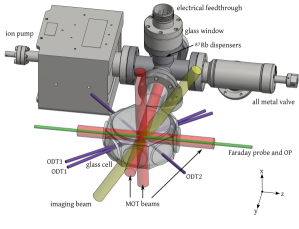
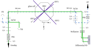
Figure 1: General setup of the experiment to form a spinor condensate in a glass cell (above). Detailed setup to perform Faraday rotation measurements of the spin state. Continuous green lines represent the Faraday beam and dashed blue lines the optical pumping beam (below).

The laser system is built up around a single “master laser” – a low noise, narrow linewidth laser that serves as a frequency reference for offset locking of the other lasers. The master laser is a $1560\text{\,}\mathrm{n}\mathrm{m}$ fiber laser (Koheras Adjustik, NKT Photonics) amplified by an erbium-doped fiber amplifier (EDFA) to a maximum power of $3\text{\,}\mathrm{W}$ (Boostik, NKT Photonics), it is frequency-doubled in a periodically-poled LiNbO₃ (PPLN) crystal of $50\text{\,}\mathrm{m}\mathrm{m}$ length. The output at $780\text{\,}\mathrm{nm}$ has a maximum power of $170\text{\,}\mathrm{mW}$ and Voigt linewidth of about $4.75(6)\text{\,}\mathrm{kHz}$ . The master laser is locked $80\text{\,}\mathrm{M}\mathrm{H}\mathrm{z}$ to the blue side of the $|F=2\rangle\rightarrow|F^{\prime}=3\rangle$ cooling transition (see Figure 2) using modulation transfer spectroscopy de Escobar et al. (2015). The cooling and repumper lasers (“slave lasers”) are extended-cavity diode lasers (ECDLs) (Toptica) which are offset locked to the master laser using an optical phase-locked loop (OPLL), as described in Appel et al. (2009), where the ultrafast photodiode is a PIN receiver (PT10GC, Bookham) and the digital phase-frequency-discriminator chip is an ADF4110 (Analog Devices) in the case of the cooler and an ADF41020 for the repumper. The chips are interfaced with a micro-controller that allows us to re-program the loops during the experiment, thereby tuning the frequency of the slave laser.

In the glass cell, a 3D magneto-optical trap (MOT) is formed with a gradient field of $11.2\text{\,}\mathrm{G}\mathrm{/}\mathrm{c}\mathrm{m}$, generated by anti-Helmholtz coils mounted around the cell along the z axis. The bias field is compensated with three pairs of Helmholtz coils in each axis. The six, circularly-polarized beams of the MOT have waists of $1\text{\,}\mathrm{c}\mathrm{m}$ (propagating along $\pm x$ and $\pm z$ directions) or $0.5\text{\,}\mathrm{c}\mathrm{m}$ (propagating along the $\pm y$ direction). Each beam contains both cooling and re-pumping light with maximum intensities of $14\text{\,}\mathrm{m}\mathrm{W}\mathrm{/}\mathrm{c}\mathrm{m}^{2}$ and $0.3\text{\,}\mathrm{m}\mathrm{W}\mathrm{/}\mathrm{c}\mathrm{m}^{2}$, respectively. The cooler beam is $15\text{\,}\mathrm{M}\mathrm{H}\mathrm{z}$ red detuned from the $|F=2\rangle\rightarrow|F^{\prime}=3\rangle$ cooling transition and the repumper is resonant with the $|F=1\rangle\rightarrow|F^{\prime}=2\rangle$ transition. The steady state number of atoms in the MOT is $10^{8}$ atoms at $200\text{\,}\mathrm{\SIUnitSymbolMicro K}$.

From the 3D MOT, the atoms are transferred to an optical dipole trap (ODT), formed at different stages of the experiment by up to three ODT beams. Each beam is linearly polarized, with wavelength $1560\text{\,}\mathrm{nm}$ and Gaussian spatial profile. ODT1 is focused to a waist of $45\text{\,}\mathrm{\SIUnitSymbolMicro m}$ at the center of the MOT, with maximum power of $11\text{\,}\mathrm{W}$ and is vertically polarized. ODT2 and ODT3 have waists $65\text{\,}\mathrm{\SIUnitSymbolMicro}\mathrm{m}$ and horizontal polarization with maximum powers $10\text{\,}\mathrm{W}$ and $7\text{\,}\mathrm{W}$ respectively. ODT1 and ODT2 propagate along the diagonals in the $y$–$z$ plane, with ODT3 at a $6^{\circ}$ angle relative to ODT1 (Figure 1). Acousto-optic modulators are used to shift ODT2 (ODT3) by $-$40\text{\,}\mathrm{M}\mathrm{H}\mathrm{z}$$ ($+$40\text{\,}\mathrm{M}\mathrm{H}\mathrm{z}$$) relative to ODT1, to avoid spatial interference. In addition, a “compensation” beam at $1529.22\text{\,}\mathrm{n}\mathrm{m}$ with up to $6\text{\,}\mathrm{mW}$ of power, mode-matched to ODT1 but of orthogonal linear polarization, can be introduced.

Because the wavelength of the ODT is close to the $1529\text{\,}\mathrm{nm}$ 3P–4D transition of ${}^{87}\mathrm{Rb}$, the ac-Stark shift of the excited 3P state is much stronger than that of the ground state. The ratio of shifts is about 47.7, which is the ratio of the scalar polarizabilities of the different states Bernon (2011). As a result, a large differential light-shift is induced on the D2 line within the ODT position and thus the cooler and repumper lasers have spatially dependent detunings (see Figure 2). We exploit this fact to form an effective dark MOT similar to that described in Clément et al. (2009): the atoms at the bottom of the potential are very unlikely to be re-pumped back into the F=2 manifold, and thus they accumulate in F=1, avoiding light-assisted collisions and radiation trapping.

ODT1 at maximum power creates a differential light shift of $312\text{\,}\mathrm{M}\mathrm{H}\mathrm{z}$ at beam center, which is larger than the hyperfine splitting between the unshifted $|F^{\prime}=2\rangle$ and $|F^{\prime}=3\rangle$ states. As a result, it is not possible to simultaneously address the cooling transition with red detuning in all spatial regions, as shown in Figure 2. To be able to continue the cooling without exciting the $|F=2\rangle\rightarrow|F^{\prime}=2\rangle$ transition during the loading of the trap we compensate the differential light shift with a $1529.22\text{\,}\mathrm{n}\mathrm{m}$ beam, which is blue detuned from the $|5P_{3/2}\rangle\rightarrow|4D_{3(5)/2}\rangle$ transitions. The light shift induced by the compensation beam in the $|5P_{3/2}\rangle$ manifold ranges from $95\text{\,}\mathrm{M}\mathrm{H}\mathrm{z}$ to $109\text{\,}\mathrm{M}\mathrm{H}\mathrm{z}$ for the different $|F^{\prime}=3,m_{F}\rangle$ sublevels, according to Floquet-theory estimates, as detailed in Coop et al. . In the presence of both $1560\text{\,}\mathrm{n}\mathrm{m}$ and the $1529.22\text{\,}\mathrm{n}\mathrm{m}$ beams, the differential light shift at the bottom of the trap is reduced to $210\text{\,}\mathrm{M}\mathrm{H}\mathrm{z}$.

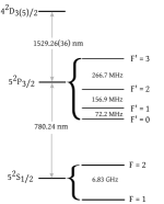
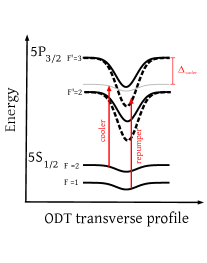
Figure 2: (left) Relevant energy levels of ${}^{87}\mathrm{Rb}$. (right) Illustration of differential light-shift as a function of the position in the optical dipole trap. Detuning of the cooler laser defined as $2\pi\Delta\equiv\omega_{\rm laser}-(\omega_{F^{\prime}}-\omega_{F})$ thus positive values of $\Delta$ indicate blue detunings from the transition. Dashed lines indicate the light-shift at full power of ODT1 with no compensation beam present, whereas continuous lines indicate the light-shift when the trap is partially compensated with the $1529.22\text{\,}\mathrm{n}\mathrm{m}$ beam.

In the partially compensated dipole trap a molasses phase is started: the magnetic field gradient is suddenly switched off, the cooling laser is further detuned to $255\text{\,}\mathrm{M}\mathrm{H}\mathrm{z}$ to the red of the unshifted $|F=2\rangle\rightarrow|F^{\prime}=3\rangle$ transition, and thus $45\text{\,}\mathrm{M}\mathrm{H}\mathrm{z}$ red-detuned at the bottom of the trap. The power of the repumper is lowered by a factor of 2.5 without changing the frequency. This phase lasts $500\text{\,}\mathrm{m}\mathrm{s}$, limited by the lifetime of the cold atom reservoir. This strategy allows us to load up to $7\text{\times}{10}^{6}\text{\,}\mathrm{a}\mathrm{t}\mathrm{o}\mathrm{m}\mathrm{s}$ in $|F=1\rangle$ at $50\text{\,}\mathrm{\SIUnitSymbolMicro}\mathrm{K}$ into the dipole trap. Using the compensation beam therefore improves the maximum number of atoms loaded by a factor of three respect to the non-compensating strategy of the ODT1 at full power, and by a factor of two loading ODT1 at a lower power for which the differential light shift does not exceed the excited-state hyperfine splitting.

After the ODT is loaded, the cooler and repumper beams are switched off and the power of the compensation beam adiabatically lowered. At the same time, a magnetic field of magnitude $B_{z}=$1\text{\,}\mathrm{G}$$ is applied along the $z$ axis. At this field, the atoms are optically pumped into the $|F=1,m_{F}=+1\rangle$ state using a beam (OP) resonant with the $|F=1\rangle\rightarrow|F^{\prime}=1\rangle$ transition and propagating along the $z$ axis with $\sigma^{+}$ polarization. We achieve $90\%$ efficiency of pumping as confirmed by Stern-Gerlach imaging along the quantization axis defined by the magnetic field. To avoid the effects of the spatially-dependent differential light shift on the atoms distributed in the trap, the optical pumping is done with three $20\text{\,}\mathrm{\SIUnitSymbolMicro}\mathrm{s}$ OP pulses during which the ODT1 is switched off. The pulses are separated by $10\text{\,}\mathrm{m}\mathrm{s}$ intervals to allow the atoms to redistribute in the trap and avoid shadowing effects.

Following optical pumping the atoms are allowed to thermalize for $500\text{\,}\mathrm{ms}$, after which the cloud is compressed in the longitudinal direction of ODT1 using ODT3. ODT3 boosts the collision rate without reducing the large collection volume. Forced all-optical evaporation in this two-beam trap is possible and efficient down to $2\text{\,}\mathrm{\SIUnitSymbolMicro}\mathrm{K}$. At that point the longitudinal frequency becomes insufficient to reach higher phase space densities. We employ an extra beam, ODT2, to provide extra compression at the end of the evaporation.

The evaporation sequence is as follows: starting with all the three beams at full power, we perform forced all-optical evaporation for $4\text{\,}\mathrm{s}$, after which the system crosses the critical temperature $T_{c}$ with about $10^{5}$ atoms. The power of ODT2 is then increased for an additional 800 ms to compress the atoms, resulting in the formation of a pure condensate with typically $4\text{\times}{10}^{4}\text{\,}\mathrm{a}\mathrm{t}\mathrm{o}\mathrm{m}\mathrm{s}$. The relative populations do not change during the evaporation, as discussed in section VI below.

III Single spin domain

A natural measure of the spatial extent of the condensate is the Thomas-Fermi radius. The mean can be expressed in terms of fundamental constants, the number of condensed atoms $N$ and the mean oscillation frequency of the harmonic trap $\bar{\omega}$:

$$\bar{R}_{\rm TF}=\left(\frac{15Na_{0}\hbar^{2}}{M^{2}\bar{\omega}^{2}}\right)^{1/5}$$ (1)

were $a_{0}=$5.38\text{\times}{10}^{-9}\text{\,}\mathrm{m}$$ is the scattering length and $M=$1.44\text{\times}{10}^{-25}\text{\,}\mathrm{k}\mathrm{g}$$ the mass of one ${}^{87}\mathrm{Rb}$ atom. The number of atoms is measured with time-of-flight absorption imaging for dense clouds Reinaudi et al. (2007).

The relative low atom number prevented direct measurement of the trap frequencies by parametric excitation. Instead we estimate $\bar{\omega}$ from the observable condensate fraction as follows: for $N$ condensed atoms of a total $N_{\rm tot}$ atoms, the condensed fraction $c_{F}=N/N_{tot}$ for non-interacting bosons obeys the relation: $c_{F}=\max[1-(T/T_{c})^{3},0]$, where the critical temperature in a harmonic trap is Pethick and Smith (2002):

$$T_{c}=\frac{\hbar\bar{\omega}}{k_{B}}\left[\frac{N_{tot}}{\zeta(3)}\right]^{1/3}$$ (2)

$k_{B}$ is the Boltzmann constant and $\zeta(3)\approx 1.202$. Time-of-flight absorption imaging and a bi-modal fit give direct access to $N_{\rm tot}$, $N$ (and thus $c_{F}$), as well as to $T$, which is found from the width of the thermal component. For fixed beam geometry and power, the trap frequencies are constant. The temperature is set by the potential depth at $T=$54(13)\text{\,}\mathrm{n}\mathrm{K}$$, independent of $N_{\rm tot}$. We can thus vary the critical temperature by changing only the number of atoms, through the duration of the ODT loading step. Figure 3 shows the condensed fraction as a function of $T/C$, where $C\equiv T_{c}/\bar{\omega}$. We fit the expected scaling of $c_{F}$ where $\bar{\omega}$ is the only free parameter, to find $\bar{\omega}=2\pi\cdot$50(5)\text{\,}\mathrm{H}\mathrm{z}$$.

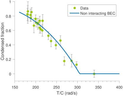
Figure 3: Condensed fraction as a function of $T/C$ where the temperature $T=$54\text{\,}\mathrm{n}\mathrm{K}$$ is constant and $C$ is a function of the number of atoms, $N_{\rm tot}$. Since only $N_{\rm tot}$varies the fit model to $c_{F}=\max\{1-[T/(C\bar{\omega}_{f})]^{3},0\}$ where $\bar{\omega}_{f}$ is the only free parameter, yielding to $\bar{\omega}=2\pi\cdot$50(5)\text{\,}\mathrm{H}\mathrm{z}$$.

The mean Thomas-Fermi radius as given by Equation 1 with $N=$4\text{\times}{10}^{4}\text{\,}$$ atoms is then: $\bar{R}_{\rm TF}=$7.0(5)\text{\,}\mathrm{\SIUnitSymbolMicro}\mathrm{m}$$. From the geometry and power of the ODT beams the shape of the condensate is expected to be a spheroid with ${R_{\rm TF}}_{1}={R_{\rm TF}}_{2}$ and anisotropy factor given by $l(t)\equiv{R_{\rm TF}}_{1}(t)/{R_{\rm TF}}_{3}(t)$. We measured the size of the condensate after $30\text{\,}\mathrm{m}\mathrm{s}$ of time-of-flight and found the final anisotropy to be $l(t=$30\text{\,}\mathrm{m}\mathrm{s}$)=$1.63(3)\text{\,}$$. Using the expansion model Castin and Dum (1996), we have estimated the initial anisotropy to be $l(t=0)=0.84$. The assumption of a spherical geometry is thus not expected to introduce large errors in what follows.

To gain some intuition about the spin-dependent contribution to the magnetization distribution the $R_{\rm TF}$ radius is compared to the spin healing length, which is defined as $\xi_{s}=\hbar/\sqrt{2M|c_{1}|n}$, where $c_{1}=$-2.39\text{\times}{10}^{-54}\text{\,}\mathrm{J}\mathrm{m}^{3}$$ characterizes the spin-dependent contact interaction, and $n$ is the density Stamper-Kurn and Ketterle (2001); Kawaguchi and Ueda (2012). In our experimental conditions, $n=$2.7\text{\times}{10}^{13}\text{\,}{\mathrm{cm}}^{-3}$$ and $\xi_{s}=$7.7\text{\,}\mathrm{\SIUnitSymbolMicro}\mathrm{m}$$, while the density healing length is $\xi_{n}=\hbar/\sqrt{2Mc_{0}n}=$0.5\text{\,}\mathrm{\SIUnitSymbolMicro}\mathrm{m}$$. Although density variations are possible since $\xi_{n}\ll\bar{R}_{\rm TF}$, spin variations in space are unlikely to occur since $\xi_{s}\sim\bar{R}_{\rm TF}$ and therefore is energetically unfavorable for the condensate to split into different spin domains,which would allow loss of coherence as the domains dephase relative to each other due to for example field gradients. In this regime the SMA can capture all the physics of the spinor condensate.

IV Excitation of spin oscillation and free oscillation

Within the SMA the order parameter can be written as $\mathbf{\hat{\Psi}}(\mathbf{r})=\varphi(\mathbf{r})\mathbf{\hat{\Psi}}$, where $\varphi(\mathbf{r})$ defines the spatial mode which is common between all the spin states. We write the spinor as $\mathbf{\hat{\Psi}}\equiv\left(\hat{\psi}_{+1},\hat{\psi}_{0},\hat{\psi}_{-1}\right)^{T}$, where $\hat{\psi}_{m_{F}}$ are the complex amplitudes describing the magnetic sublevels Law et al. (1998b). The atoms condense in $|F=1,m_{F}=+1\rangle$ so initially $\mathbf{\hat{\Psi}}=\left(1,0,0\right)^{T}$.

From this initial state, we lower $B_{z}$ to zero while increasing the field along $x$ to a maximum value $B_{x}$. This is done slowly compared to the Larmor frequency defined by the field amplitude so the spins adiabatically follow the field and finish pointing along $x$. To rotate the spins to the $y$–$z$ plane and form the state $\frac{1}{2}\left(1,\sqrt{2},1\right)^{T}$, a $\pi/2$-RF pulse along $y$ is applied. This starts Larmor precession dynamics around the $x$ axis with a Larmor frequency $\omega_{L}=\gamma B_{x}$, where $\gamma=2\pi($-0.7\text{\,}\mathrm{M}\mathrm{H}\mathrm{z}\mathrm{/}\mathrm{G}$)$ is the gyromagnetic ratio of ${}^{87}\mathrm{Rb}$ in the $F=1$ manifold.

While the dominant effect on the spin dynamics is the linear Zeeman shift, which produces a Larmor precession about $x$, the quadratic Zeeman shift also plays a significant role, and manifests as a modulation of the Larmor precession. As described below, the $z$ projection of the spin evolves as $\langle{f}_{z}\rangle(t)=\cos\Theta_{L}\cos\Theta_{Q}$ where $\Theta_{L,Q}\equiv\int dt\,\omega_{L,Q}(t)$ and $\omega_{Q}=\hbar\gamma^{2}B^{2}/\Delta E_{\rm hf}$, with $\Delta E_{\rm hf}=2\pi\hbar\times$6.83\text{\,}\mathrm{G}\mathrm{H}\mathrm{z}$$ being the hyperfine splitting Stamper-Kurn and Ueda (2013).

A single atom exposed to a magnetic field $B_{x}(t)$ along the $x$ direction experiences the spin Hamiltonian

$$\hat{H} = \frac{g_{J}\mu_{B}}{4}B_{x}\hat{f}_{x}+\frac{g_{J}^{2}\mu_{B}^{2}}{16\Delta E_{\rm hf}}B_{x}^{2}\hat{f}_{x}^{2}+O(B_{x}^{3})$$ (3)

$$\equiv \hbar\omega_{L}\hat{f}_{x}+\hbar\omega_{Q}\hat{f}_{x}^{2}+O(B_{x}^{3})$$

where $\hat{f}_{\alpha}$ denotes the spin-1 Pauli matrix for component $\alpha\in\{x,y,z\}$ Colangelo et al. (2013).We note that $B_{x}$ and thus $\omega_{L},\omega_{Q}$ may be time-dependent. Due to the $\hat{f}_{x}^{2}$ term the dynamics induced by the Hamiltonian involves both, the vector “spin orientation” components $\hat{f}_{x},\hat{f}_{y},\hat{f}_{z}$, and the rank-two tensor “spin-alignment” components:

$$\hat{\jmath}_{zx} \equiv \hat{f}_{z}\hat{f}_{x}+\hat{f}_{x}\hat{f}_{z},$$ (4)

$$\hat{\jmath}_{xy} \equiv \hat{f}_{x}\hat{f}_{y}+\hat{f}_{y}\hat{f}_{x}.$$ (5)

We find the single-atom equations of motion

$$\frac{d}{dt}\left(\begin{array}[]{c}f_{x}\\ f_{y}\\ f_{z}\\ j_{zx}\\ j_{xy}\end{array}\right) = \left(\begin{array}[]{ccccc}0&0&0&0&0\\ 0&0&-\omega_{L}&-\omega_{Q}&0\\ 0&\omega_{L}&0&0&\omega_{Q}\\ 0&\omega_{Q}&0&0&\omega_{L}\\ 0&0&-\omega_{Q}&-\omega_{L}&0\end{array}\right)\left(\begin{array}[]{c}f_{x}\\ f_{y}\\ f_{z}\\ j_{zx}\\ j_{xy}\end{array}\right)$$ (21)

which describe a pair oscillators, $f_{y}$–$f_{z}$ and $j_{zx}$–$j_{xy}$, each with oscillation frequency $\omega_{L}$, and mutual coupling frequency $\omega_{Q}$.

The collective spin of $N$ condensed atoms is ${\bf F}\equiv\sum_{n=1}^{N}{\bf f}^{(n)}$, where the superscript indicates the $n$th atom The dynamics of the collective spin then obeys

$$\hat{F}_{i}(t) = N(t)\hat{f}_{i}(t)$$ (22)

which describes the coherent oscillation of a macroscopic spin, and its decay caused by the loss of atoms. This is studied further in section VI.

V Non-destructive probing of the spin polarization

We perform non-destructive Faraday rotation measurements of the spin state of the atoms, exploiting the spin-dependent interaction of a linearly polarized off-resonant beam with the vectorial component of the atomic polarizability, as described in Koschorreck et al. (2010). The interaction with the atoms causes the linear polarization of this beam to rotate and therefore to acquire a diagonal component, which is detected using a shot-noise limited polarimeter based on the differential photodetector (DFD) described in Ciurana et al. (2016). We have demonstrated the differential photodetector is shot-noise limited for $\text{\,}\mathrm{\SIUnitSymbolMicro s}$ pulses with $2\text{\times}{10}^{5}$ to ${10}^{7}\text{\,}\mathrm{p}\mathrm{h}\mathrm{o}\mathrm{t}\mathrm{o}\mathrm{n}\mathrm{s}$, having an electronic noise floor equivalent to the shot noise of a pulse with $2.6(5)\text{\times}{10}^{5}\text{\,}\mathrm{p}\mathrm{h}\mathrm{o}\mathrm{t}\mathrm{o}\mathrm{n}\mathrm{s}$, as shown in Figure 4.

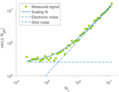
Figure 4: Variance of the output signal of the differential photodetector as a function of total input number of photons ($N_{L}$). The fit assumes the form $\mathrm{var}\left(\Delta N_{\rm diff}\right)=V_{e}+N_{L}$ to find the electronic noise floor $V_{e}=$2.6(5)\text{\times}{10}^{5}$$.

The Faraday beam is red detuned $276\text{\,}\mathrm{M}\mathrm{H}\mathrm{z}$ from the $|F=1\rangle\rightarrow|F^{\prime}=0\rangle$ transition and has linear polarization of $54.7\mathrm{°}$ with respect to the bias field along $x$. At this “magic angle” the tensorial AC stark shift averages to zero over one precession cycle Smith et al. (2004), enabling continuous probing without conversion of spin alignment to spin orientation.

The Faraday probing is typically performed with $\tau_{p}=$10\text{\,}\mathrm{\SIUnitSymbolMicro}\mathrm{s}$$ pulses containing $N_{L}=5\times 10^{6}$ photons. To compensate probe power fluctuations, $N_{L}$ is measured by splitting a fraction of the power to an auxiliary PD and transimpedance amplifier before entering the chamber. An example of the Faraday rotation signal is shown in Figure 5. The polarization rotation angle in the Poincaré sphere $\phi=G_{1}F_{z}$ is proportional to the collective spin component $F_{z}$, and with a coupling $G_{1}$ that depends on the overlap of the beam and the atomic cloud. For this reason, the probing beam is focused at the atoms position with a waist of $18\text{\,}\mathrm{\SIUnitSymbolMicro}\mathrm{m}$. For the pure condensate, we observe $G_{1}=${10}^{-7}\text{\,}\mathrm{r}\mathrm{a}\mathrm{d}\mathrm{/}\mathrm{s}\mathrm{p}\mathrm{i}\mathrm{n}$$, by measuring the rotation angle caused by a fully polarized cloud with a known number of spins calibrated with absorption imaging.

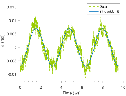
Figure 5: Example of Faraday rotation angle along the probing direction z. In this example, the probing pulse contains $5\text{\times}{10}^{6}\text{\,}\mathrm{p}\mathrm{h}\mathrm{o}\mathrm{t}\mathrm{o}\mathrm{n}\mathrm{s}$ and the magnetic field is such that the Larmor frequency is $\omega_{L}=2\pi\cdot$300\text{\,}\mathrm{k}\mathrm{H}\mathrm{z}$$. The coupling constant is such that $\phi(t)=(${10}^{-7}\text{\,}\mathrm{r}\mathrm{a}\mathrm{d}\mathrm{/}\mathrm{s}\mathrm{p}\mathrm{i}\mathrm{n}$)F_{z}(t)$.

The known shot-noise scaling of the optical angle allows us to estimate for one pulse with $N_{L}=$5\text{\times}{10}^{6}\text{\,}\mathrm{p}\mathrm{h}\mathrm{o}\mathrm{t}\mathrm{o}\mathrm{n}\mathrm{s}$$ an optical angle noise of $d\phi=1/\sqrt{N_{L}}=$0.4\text{\,}\mathrm{m}\mathrm{r}\mathrm{a}\mathrm{d}$$, which corresponds to an inferred noise in the spin state $\sqrt{\mathrm{var}\left(F_{z}\right)}=(G_{1}\sqrt{N_{L}})^{-1}\simeq$4\text{\times}{10}^{3}\text{\,}\mathrm{s}\mathrm{p}\mathrm{i}\mathrm{n}\mathrm{s}$$. The noise is larger than the projection noise inherent to the atomic state, which is given by $\sqrt{\mathrm{var}\left(F_{z}\right)}=\sqrt{N}=$2\text{\times}{10}^{2}\text{\,}\mathrm{s}\mathrm{p}\mathrm{i}\mathrm{n}\mathrm{s}$$. The interaction with each pulse does not cause atoms to be lost from the trap, but it kicks atoms out from the condensate reducing the condensed fraction by $25\%$. Reaching low damage projection noise limited measurements requires improvement to the coupling factor $G_{1}$ rather than using more photons.

VI Spin coherence properties of the spinor BEC

In other spin systems, e.g. liquid-state magnetic resonance Bloembergen et al. (1948), it is common to distinguish a relaxation rate $1/\mathcal{T}_{1}$ for the longitudinal spin component, i.e., the one parallel to the field, and distinct transverse relaxation rates $1/\mathcal{T}_{2}$ due to only homogeneous effects (relevant for spin-echo experiments), and $1/\mathcal{T}_{2}^{*}$ for relaxation due to both homogeneous and inhomogeneous effects. Here, in contrast, the single-mode condition implies a single spin state $\mathbf{\hat{\Psi}}(t)$ for the entire condensate, enforcing full coherence. We thus expect $\mathcal{T}_{2}=\mathcal{T}_{2}^{*}=\mathcal{T}_{1}$, with $\mathcal{T}_{1}$ limited only by loss of atoms from the condensate, to which we assign a rate $1/\mathcal{T}_{0}$.

Atom losses: Atom losses are caused by collisions with the background gas and by three-body collisions. The former knock condensate atoms out of the trap, or less frequently into the thermal cloud. The latter are strongly exothermic and result in loss of all three atoms. The atom number in the condensate evolves as

$$\dot{N}=-N/\tau-K_{3}\int d^{3}x\,n^{3}(x,t)$$ (23)

where the first term describes loss from background collisions and the second from three-body losses Burt et al. (1997); Söding et al. (1999). For condensed atoms of ${}^{87}\mathrm{Rb}$ , $K_{3}\simeq$6\text{\times}{10}^{-30}\text{\,}\mathrm{c}\mathrm{m}^{6}\mathrm{/}\mathrm{s}$$ so that at our densities of $n\simeq$3\text{\times}{10}^{13}\text{\,}{\mathrm{cm}}^{-3}$$, the three-body loss rate is of order $K_{3}n^{2}N\simeq N/$200\text{\,}\mathrm{s}$$. In contrast, the observed number decay, measured by absorption imaging, is much faster, and well described by one-body losses with $\mathcal{T}_{1}=\tau=$7.7(4)\text{\,}\mathrm{s}$$. The three-body loss can thus be neglected in these conditions.

Longitudinal spin relaxation: Under the Hamiltonian of Equation 3 above, both $f_{x}$ and the magnetic quantum number $m_{F}$ (in the $x$-basis) are constants of the motion, even for fluctuating $B_{x}(t)$. This we confirm using Stern-Gerlach imaging to measure the population in the different magnetic sublevels as a function of hold time: a condensate is prepared in the $\left(1,0,0\right)^{T}$ state and held in the dipole trap during a time $t_{e}$, after which the atoms are released from the trap. During the time of flight a gradient field of $\sim$20\text{\,}\mathrm{G}\mathrm{/}\mathrm{c}\mathrm{m}$$ is applied for $10\text{\,}\mathrm{m}\mathrm{s}$ to spatially separate the different spin components, before performing absorption imaging. The relative populations of the different spin states remain unchanged as a function of $t_{e}$, to within measurement precision.

We note that orthogonal AC magnetic fields at a frequency close to $\omega_{L}$ could resonantly excite transitions among $m_{F}$ levels. The influence of such fields has limited the observation of spin dynamics in other experiments Chang et al. (2004). In our experiment this effect becomes evident only at bias fields below $100\text{\,}\mathrm{m}\mathrm{G}$.

Transverse spin relaxation: Very long coherence times require very stable bias fields to estimate $\mathcal{T}_{2}^{*}$ by direct measurement of $\langle F_{z}(t)\rangle$. A change in the magnetic field between repetitions of the experiment generates a $F_{z}(t)$ with a different phase $\Theta_{L}$, and the average shows a relaxation-like behaviour $\langle F_{z}(t)\rangle\propto\exp[-\tau/\overline{\mathcal{T}_{2}}]$, where $\overline{\mathcal{T}_{2}}$ is a relaxation time related to the shot-to-shot variation of the field, and only weakly related to the processes described by $\mathcal{T}_{2}^{*}$. Using a fluxgate sensor, we measured the spectrum of environmental magnetic noise near the atoms. Simulating the spin dynamics for such variations of the magnetic field we estimate $\overline{\mathcal{T}_{2}}=$1.3\text{\,}\mathrm{m}\mathrm{s}$$.

To accurately measure $\mathcal{T}_{2}^{*}$ in such circumstances, we take advantage of the non-destructive nature of the Faraday rotation probing, which allows us to probe several Larmor cycles of $F_{z}(t)$ during a single run and extract the amplitude via a sinusoidal fit. Because the amplitude does not depend on $\Theta_{L}$, this allows meaningful averaging in spite of the shot-to-shot fluctuations. The quadratic phase $\Theta_{Q}$ also varies shot-to-shot, but on a time-scale about four orders of magnitude longer than does $\Theta_{L}$, implying that the average amplitude will show effects of dephasing on the $10\text{\,}\mathrm{s}$ time scale.

We prepare the state $\frac{1}{2}\left(1,\sqrt{2},1\right)^{T}$ and allow the atoms precess around the bias field $B_{x}=$0.29\text{\,}\mathrm{G}$$ for time $t_{e}$, before $F_{z}(t)$ is measured for $10\text{\,}\mathrm{\SIUnitSymbolMicro}\mathrm{s}$ allowing several Larmor cycles to be resolved by fitting a sinusoidal function as in Figure 5. We perform measurements at different values of $t_{e}$ ranging from $0$ to $1\text{\,}\mathrm{s}$, each one on a new preparation of the state. The Larmor frequency is always $(\omega_{L}=2\pi\cdot$200\text{\,}\mathrm{k}\mathrm{H}\mathrm{z}$)$. To separate the relaxation and decoherence signature from the atomic losses, we normalized the signal by the number of atoms measured by absorption imaging at the end of each repetition.

In Figure 6 we plot the mean square amplitude of the sinusoidal fits for different repetitions, as a function of $t_{e}$. To this data we fit a function $A\cos^{2}(\omega_{Q}t)\exp{(-2t/\mathcal{T})}$, from which we find $\omega_{Q}=2\pi\cdot$5.95(1)\text{\,}\mathrm{H}\mathrm{z}$$ and $\mathcal{T}\gg$1\text{\,}\mathrm{s}$$, much longer than the observation time, which implies $\langle F_{z}\rangle$ is only limited by the atom losses and therefore $\mathcal{T}_{2}^{*}\simeq\mathcal{T}_{0}$. As can be appreciated in the figure, the full visibility is always recovered even at observation times as long as $1\text{\,}\mathrm{s}$.

With these results we confirm $\mathcal{T}_{2}^{*},\mathcal{T}_{2},\mathcal{T}_{1}\gg$1\text{\,}\mathrm{s}$$. That is, we observe no relaxation or decoherence mechanism degrading the coherence of the state in the observed time scales. The result is consistent with the expectation of spin relaxation due solely to atom losses, which in our typical vacuum conditions is limited by one-body losses $\mathcal{T}_{2}^{*}\simeq\mathcal{T}_{2}\simeq\mathcal{T}_{1}\simeq\mathcal{T}_{0}=$7.7(4)\text{\,}\mathrm{s}$$.

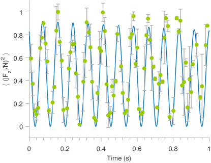
Figure 6: Average over different repetitions of the normalized z spin projection square vs evolution time (s). The signals are obtained using Faraday rotation measurements of a fully polarized condensate. The spins rotate around $x$ at Larmor precession frequency $\omega_{L}=2\pi\cdot$200\text{\,}\mathrm{k}\mathrm{H}\mathrm{z}$$ with a quadratic component oscillating at $\omega_{Q}=2\pi\cdot$6\text{\,}\mathrm{H}\mathrm{z}$$. We observe negligible decay of the normalized magnetization, which implies $\mathcal{T}_{2}^{*}\simeq\mathcal{T}_{0}$.

VII Conclusions

This work reports on the construction of a minimalist system capable of creating single-mode spinor Bose-Einstein condensates of ${}^{87}\mathrm{Rb}$ atoms in the ferromagnetic $F=1$ hyperfine state. The loading of the dipole trap involves a novel technique where the differential light shift induced by the dipole trap is exploited to create an effective dark-MOT. Based on measurements of the spatial size, densities and coherence, we demonstrate the spinor condensate is created in a single spin domain, because there are not different domains the collective spin does not dephase in the time scales limited by the lifetime of the condensate. We have demonstrated one second of coherence of the collective spin state and inferred several seconds of coherence via non-destructive probing of the spin state based on Faraday rotation measurements. The noise of the probing is close to the atomic projection noise inherent to the spin state. The long coherence together with the small size, situate the system in a very promising position for applications including coherent sensing of magnetic fields.

References

- Sadler et al. (2006) L. E. Sadler, J. M. Higbie, S. R. Leslie, M. Vengalattore, and D. M. Stamper-Kurn, Nature 443, 312 (2006), 10.1038/nature05094.
- Gu et al. (2004) Q. Gu, K. Bongs, and K. Sengstock, Phys. Rev. A 70, 063609 (2004).
- Eto et al. (2014) Y. Eto, H. Saito, and T. Hirano, Phys. Rev. Lett. 112, 185301 (2014).
- Choi et al. (2012) J.-y. Choi, W. J. Kwon, and Y.-i. Shin, Phys. Rev. Lett. 108, 035301 (2012).
- Pietilä and Möttönen (2009) V. Pietilä and M. Möttönen, Phys. Rev. Lett. 103, 030401 (2009).
- Ray M. W. et al. (2014) Ray M. W., Ruokokoski E., Kandel S., Mottonen M., and Hall D. S., Nature 505, 657 (2014).
- Cirac et al. (1998) J. I. Cirac, M. Lewenstein, K. Mølmer, and P. Zoller, Phys. Rev. A 57, 1208 (1998).
- Higbie and Stamper-Kurn (2004) J. Higbie and D. M. Stamper-Kurn, Phys. Rev. A 69, 053605 (2004).
- Kawaguchi et al. (2006) Y. Kawaguchi, H. Saito, and M. Ueda, Phys. Rev. Lett. 96, 080405 (2006).
- Gawryluk et al. (2007) K. Gawryluk, M. Brewczyk, K. Bongs, and M. Gajda, Phys. Rev. Lett. 99, 130401 (2007).
- Law et al. (1998a) C. K. Law, H. Pu, N. P. Bigelow, and J. H. Eberly, Phys. Rev. A 58, 531 (1998a).
- Duan et al. (2002) L.-M. Duan, J. I. Cirac, and P. Zoller, Phys. Rev. A 65, 033619 (2002).
- Müstecaplıoğlu et al. (2002) Ö. E. Müstecaplıoğlu, M. Zhang, and L. You, Phys. Rev. A 66, 033611 (2002).
- Budker and Romalis (2007) D. Budker and M. Romalis, Nature Phys. 3, 227 (2007).
- Vengalattore et al. (2007) M. Vengalattore, J. M. Higbie, S. R. Leslie, J. Guzman, L. E. Sadler, and D. M. Stamper-Kurn, Phys. Rev. Lett. 98, 200801 (2007).
- Muessel et al. (2014) W. Muessel, H. Strobel, D. Linnemann, D. B. Hume, and M. K. Oberthaler, Phys. Rev. Lett. 113, 103004 (2014).
- Brask et al. (2015) J. B. Brask, R. Chaves, and J. Kołodyński, Phys. Rev. X 5, 031010 (2015).
- Koashi and Ueda (2000) M. Koashi and M. Ueda, Physical Review Letters 84, 1066 (2000).
- Yi et al. (2002) S. Yi, Ö. E. Müstecaplıoğlu, C. P. Sun, and L. You, Phys. Rev. A 66, 011601 (2002).
- Corre et al. (2015) V. Corre, T. Zibold, C. Frapolli, L. Shao, J. Dalibard, and F. Gerbier, EPL (Europhysics Letters) 110, 26001 (2015).
- Kronjäger et al. (2005) J. Kronjäger, C. Becker, M. Brinkmann, R. Walser, P. Navez, K. Bongs, and K. Sengstock, Physical Review A 72, 063619 (2005).
- Burt et al. (1997) E. A. Burt, R. W. Ghrist, C. J. Myatt, M. J. Holland, E. A. Cornell, and C. E. Wieman, Phys. Rev. Lett. 79, 337 (1997).
- Söding et al. (1999) J. Söding, D. Guéry-Odelin, P. Desbiolles, F. Chevy, H. Inamori, and J. Dalibard, Applied Physics B 69, 257 (1999).
- Miesner et al. (1999) H.-J. Miesner, D. Stamper-Kurn, J. Stenger, S. Inouye, A. Chikkatur, and W. Ketterle, Physical Review Letters 82, 2228 (1999).
- Schmaljohann et al. (2004) H. Schmaljohann, M. Erhard, J. Kronjäger, M. Kottke, S. Van Staa, L. Cacciapuoti, J. Arlt, K. Bongs, and K. Sengstock, Physical Review Letters 92, 040402 (2004).
- Note (1) The linewidth was estimated from the measurement of the linewidth of the laser in a self-heterodyne interferometer with a delay line. The analysis assumes the model proposed in Mercer (1991) where the noise is modeled by white noise plus a component, which is due to thermal fluctuations. The first source of noise gives a Lorentzian character to the linewidth whereas the second one is Gaussian to good approximation. The convolution of both contributions results in a Voigt profile.
- de Escobar et al. (2015) Y. N. M. de Escobar, S. P. Álvarez, S. Coop, T. Vanderbruggen, K. T. Kaczmarek, and M. W. Mitchell, Opt. Lett. 40, 4731 (2015).
- Appel et al. (2009) J. Appel, A. MacRae, and A. I. Lvovsky, Meas. Sci. Technol. 20, 055302 (2009).
- Bernon (2011) S. Bernon, Piégeage et mesure non-destructive d’atomes froids dans une cavité en anneau de haute finesse, Ph.D. thesis (2011), thèse de doctorat dirigée par Bouyer, Philippe Physique Palaiseau, Ecole polytechnique 2011.
- Clément et al. (2009) J.-F. Clément, J.-P. Brantut, M. Robert-de Saint-Vincent, R. A. Nyman, A. Aspect, T. Bourdel, and P. Bouyer, Phys. Rev. A 79, 061406 (2009).
- (31) S. Coop, S. Palacios, P. Gomez, Y. N. Martinez de Escobar, T. Vanderbruggen, and M. W. Mitchell, arXiv:1702.02802 [physics.atom-ph] .
- Reinaudi et al. (2007) G. Reinaudi, T. Lahaye, Z. Wang, and D. Guéry-Odelin, Opt. Lett. 32, 3143 (2007).
- Pethick and Smith (2002) C. J. Pethick and H. Smith, Bose-Einstein condensation in dilute gases (Cambridge University Press, 2002).
- Castin and Dum (1996) Y. Castin and R. Dum, Phys. Rev. Lett. 77, 5315 (1996).
- Stamper-Kurn and Ketterle (2001) D. Stamper-Kurn and W. Ketterle, Coherent atomic matter waves , 139 (2001).
- Kawaguchi and Ueda (2012) Y. Kawaguchi and M. Ueda, Physics Reports 520, 253 (2012).
- Law et al. (1998b) C. K. Law, H. Pu, and N. P. Bigelow, Phys. Rev. Lett. 81, 5257 (1998b).
- Stamper-Kurn and Ueda (2013) D. M. Stamper-Kurn and M. Ueda, Rev. Mod. Phys. 85, 1191 (2013).
- Colangelo et al. (2013) G. Colangelo, R. J. Sewell, N. Behbood, F. M. Ciurana, G. Triginer, and M. W. Mitchell, New Journal of Physics 15, 103007 (2013).
- Koschorreck et al. (2010) M. Koschorreck, M. Napolitano, B. Dubost, and M. W. Mitchell, Phys. Rev. Lett. 104, 093602 (2010).
- Ciurana et al. (2016) F. M. Ciurana, G. Colangelo, R. J. Sewell, and M. W. Mitchell, Opt. Lett. 41, 2946 (2016).
- Smith et al. (2004) G. A. Smith, S. Chaudhury, A. Silberfarb, I. H. Deutsch, and P. S. Jessen, Phys. Rev. Lett. 93, 163602 (2004).
- Bloembergen et al. (1948) N. Bloembergen, E. M. Purcell, and R. V. Pound, Phys. Rev. 73, 679 (1948).
- Chang et al. (2004) M.-S. Chang, C. D. Hamley, M. D. Barrett, J. A. Sauer, K. M. Fortier, W. Zhang, L. You, and M. S. Chapman, Phys. Rev. Lett. 92, 140403 (2004).
- Mercer (1991) L. Mercer, Journal of Lightwave Technology 9, 485 (1991).