UHECR primary identification using the lateral profile of muons in EAS

Abstract

New developments in detector technology allow for a realistic cost of large area surface detectors for cosmic ray air showers, with some limitations on particle identification, energy resolutions, directional information and dynamic range. In this paper, we present a simulation study using CORSIKA to quantify the lateral profile of the muons at ground level, characterized by their energy spectrum and lateral spread, and combine it with the depth at shower maximum (X_max) of an EAS initiated by a primary at energies $10^{16}$ eV – $10^{19}$ eV. Using different primaries, we show that the combined muon observables and X_max can identify the primary in a large fraction of the events, depending on the energy and the detector performance. This study provides important input parameters for the design of a future muon detector for surface array, which will be able to boost the knowledge of primaries and of the QCD interactions in the atmosphere.

1 Introduction

The Ultra High Energy Cosmic Rays (UHECRs) are the most energetic particles known, and their origin and composition are not well understood yet [1, 2, 3, 4, 5]. The detection of the UHECRs is difficult owing to the fact that their flux at higher energies is very low, and the only way to detect them is by observing the large cascades of secondary particles, known as the Extensive Air Showers (EAS), which are produced by the interaction of these cosmic rays with the atmosphere. The direct detectors placed in balloons or satellites, capable of probing the composition of cosmic primaries, reach energy up to about $10^{14.5}$ eV only [6, 7, 8, 9, 10, 11, 12, 13, 14, 15, 16, 17, 18]. The state of the art experiments to detect the UHECRs are yet to be able to study all the key observables required. The energy and the incident direction of the primary cosmic rays into the atmosphere are reconstructed with precision, however, the composition of the primary mass remains an open question [19, 20, 21, 22, 23, 24]. The composition at different energies has strong implications on the sources, which are not completely known, the propagation, and possible interpretation of new physics involved at the highest energies. The galactic and extragalactic magnetic fields, the location of the source and its density evolution are still debated [25, 26, 27, 28, 29]. Establishing the mass composition at the high and ultra high energies, from the astrophysical reasons, bear fundamental importance as it would provide information on various origins and propagation of the cosmic rays [30, 31, 32, 33, 34, 35, 36, 37, 38]. A related question is the hadronic interactions at ultra high energies, beyond the reach of current accelerators, governing the initial evolution of the EAS. The hadronic interactions are parameterized by various models, however, at the highest energies all exhibit significant uncertainties.

The muons in an Extensive Air Shower are sensitive to the primary composition and to the hadronic interaction properties. The muons are produced essentially from decaying charged mesons, and can be a fundamental tool to map the high energy hadronic interaction, as the individual particle signature is not washed out as in the electromagnetic component. In a typical EAS, muons represent about 10% of all the charged particles. A large fraction of the muons reach the ground due to a low interaction cross section and a long decay time, and they have a wide lateral distribution. Most of the muons are produced in the upper atmosphere, typically 15 km above ground level, and lose about 2 GeV of their energy to ionization by the time they reach the ground. The energy and angular distribution of the muons reaching the ground depends on the production spectrum, their energy loss through the atmosphere and decays. For negligible muon decay (E${}_{\mu}\textgreater$ 100/$\cos\theta$ GeV), negligible curvature of the Earth ($\theta~{}\textless~{}70^{\circ}$) the overall muon number spectrum can be expressed by an approximate extrapolation formula, [39, 40]

$$\frac{dN_{\mu}}{dE_{\mu}d\Omega}\approx\frac{0.14~{}E_{\mu}^{-2.7}}{\rm cm^{2}~{}s~{}sr~{}GeV}\Bigg{\{}\frac{1}{1+\frac{1.1~{}E_{\mu}\cos\theta}{115~{}\rm GeV}}+\frac{0.054}{1+\frac{1.1~{}E_{\mu}\cos\theta}{850~{}\rm GeV}}\Bigg{\}}.$$ (1.1)

Here, the two terms give the contribution of pions and charged kaons respectively. The contribution from charm and heavier flavors are negligible except at very high energy, and is neglected in this formula.

The approximate expression for the total number of muons (N_μ) at energies above 1 GeV, given by Greisen [41], is

$$N_{\mu}(\textgreater~{}1~{}\rm GeV)\approx 0.95\times 10^{5}\bigg{(}\frac{N_{c}}{10^{6}}\bigg{)}^{3/4},$$ (1.2)

where $N_{c}$ is the total number of charged particles in the shower.

The lateral spread of the muons would be larger than the other charged particles, and would depend on the factors like the transverse momenta of the muons at the point of their production and muon–multiple scattering. The spread has large fluctuation shower to shower, even showers with identical primary mass and energy. The number of muons per square meter $\rho_{R}$, as a function of the lateral distance R (m) from the core of the shower is expressed as

$$\rho_{R}=\frac{dN_{\mu}}{dR^{2}}[R]=\frac{1.25~{}\rm N_{\mu}}{2\pi\Gamma(1.25)}\bigg{(}\frac{1}{320}\bigg{)}^{1.25}R^{-0.75}\bigg{(}1+\frac{r}{320}\bigg{)}^{-2.5},$$ (1.3)

where $\Gamma$ is the gamma function.

Large area detectors and appropriate discrimination against the much more abundant electromagnetic particles are needed for muon detection. The measurement of the individual charged particles in an extensive air shower (EAS), at a surface detector array, would provide important distinguishing parameters to identify the cosmic primary particle. These will also contribute to the mapping of the very high energy interactions in the topmost layers of the atmosphere, i.e., beyond the reach of current accelerators, and to probe anomalies beyond QCD. The ongoing attempts to study individual muons are limited in their expandability to larger arrays [42, 43].

New developments in detector technology allow for a realistic cost of large area detectors. Examples of these are gas filled photon sensors such as THGEMs [44] or resistive plate WELL [45, 46], as well as other techniques developed worldwide such as Resistive Plate Chambers [47]. The long term stability of these solutions is improving gradually, which is a major step for surface array applications. The application for a muon detector is possible through use of Ring Imaging Cerenkov, varying Cerenkov thresholds or others, and would require specific design based on the desired performance. A major part of the work performed in this paper is aimed at identifying the requirements in terms of energy, temporal and spatial resolutions that would suffice for important insights to cosmic ray physics.

This work aims at advancing towards primary identification, shower–by–shower, with the observables of the muon component of an EAS. The energy and position of the muons in a simulated EAS, combined with the depth at shower maximum, $X_{max}$, and the energy of the primary $E_{p}$, are used in a log likelihood analysis to distinguish the primaries. The paper is organized in the following way. Section (2) describes the simulation. In Section (3), the parametrization of the muon component of an EAS are described. Section (4) discusses the results in distinguishing the showers from light and heavy primaries, choosing protons and Fe to be representative of the two groups. Finally, in Section (5), a brief summary of the work is presented with remarks on its possible application.

2 Simulation details

In this section, we describe about the details of the air shower simulation.

2.1 EAS simulation

Here we describe the simulation of the EAS events and their translation in a horizontal array of detectors. The extensive air showers, initiated by cosmic ray primaries of different masses, energies and directions, are generated in CORSIKA Monte Carlo program [48]. CORSIKA studies in detail how an EAS evolves in the atmosphere, and allows to simulate the interactions and decays of nuclei, electrons, photons, hadrons and muons. CORSIKA contains several models and generators to treat the high energy hadronic interactions, namely the DUAL Parton Model (DPMJET)[49], the quark-gluon-string model (QGSJET01) [50, 51], the mini jet model SIBYLL [52, 53], VENUS[54], NEXUS [55], EPOS LHC [56], and QGSJETII-04 [57, 58]. The low energy hadronic interactions are simulated with one of FLUKA [59], GHEISHA [60] or UrQMD [61] models. The type, energy, location, direction and arrival time of all the secondary particles up to thinning level are the outputs of this program. In CORSIKA, all particle decay branches down to 1% are taken into account. Thinning is not used for muons, as we follow each separately. We choose a few primaries and generate showers for different primary energies and zenith angles. Some of the parameters used in simulating the air showers are listed in table 1.

Parameter	Value
Version	7.4
Primary Particle	proton, Fe
	Group I ( A $\leq$ 4 )
	Group II (4 $\textless$ A $\leq$ 25 )
	Group III (25 $\textless$ A $\leq$ 56)
Zenith Angle	$0^{\circ}~{}\pm~{}2.5^{\circ}$
Azimuth Angle	$-180^{\circ}$ to $180^{\circ}$
Slope of primary energy spectrum	-2.7
Starting Altitude	0
Observation level	110 m above sea level
Earth’s Magnetic field	$B_{x}$ = 20.40 $\mu$T
	$B_{z}$ = 43.23 $\mu$T
Hadronic interaction model ($\textless$ Ecm = 12 GeV)	GHEISHA
Hadronic interaction model ($\textgreater$ Ecm = 12 GeV)	QGSJET II–04
	SIBYLL
	EPOS
Lowest energy cut-off for hadrons (without $\pi^{0}$)	0.3 GeV
Lowest energy cut-off for muons	0.3 GeV
Lowest energy cut-off for electrons	0.003 GeV
Lowest energy cut-off for photons (including $\pi^{0}$)	0.003 GeV

Table 1: The values of some parameters used in CORSIKA–simulation

2.2 Detection

The information (energy, direction, location) of the secondary muons produced in an EAS is then translated through an array of 2 m $\times$ 2 m detectors. We consider various scenarios of the separation between the detector stations, to collect 100% (no separation), 1% (20 m), 0.16% (50 m) and 0.01% (200 m) of the muons. Apart from the case of an ideal muon detector with 100% detection efficiency and ideal energy resolution, the detector characteristics were varied so that we analyze the prospect of a realistic detector. The muon energy range used in the analysis is 0.5 GeV – 50 GeV.

3 The lateral spread of the muons in EAS

In this study, the lateral distribution at ground lever of the muons originating from an air shower is probed for different primary mass species. The difference in the average distributions for cosmic primaries is an important distinguishing parameter and is used to develop a statistical toolkit to identify the mass of the primaries.

3.1 The average muon number density (lateral) as a function of ($E_{\mu}$, $R$, $X_{max}$)

We start with comparing the number of muons in proton and Fe initiated showers. In figure 1, we show the dependence of the number of muons ($N_{\mu}$) as a function of $X_{max}$, at a few chosen segments in $E_{\mu}$ and $R$. It can be seen from figure 1 that, the variation in $N_{\mu}$ and its behavior with $X_{max}$ is significant even at a reasonable distance from the shower core. This is an important feature for this study.

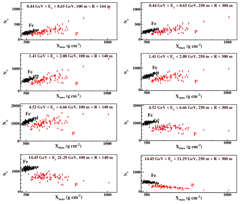
Figure 1: The number of muons $N_{\mu}$, at a few chosen ($E_{\mu}$, R) bins, as a function of $X_{max}$ for showers with $E_{p}$ = 10¹⁶ eV, $\theta_{p}~{}=~{}0^{\circ}~{}\pm~{}2.5^{\circ}$. The red dots represent the showers from Fe primaries, while the black dots represent those from proton primaries.

In this work we obtain a correlation among the muon energy, the lateral position of the muons with respect to the shower core, and the $X_{max}$ of the shower. All these parameters have significant fluctuation shower-to-shower. 100 showers for proton and Fe each are used for best fitting. Using the simulated events, we calculate the average lateral number density ${\rho}_{ER^{2}}$ (per GeV per square meter) of the muon shower as a function of $E_{\mu}$ (GeV), R (m) and $X_{max}$. We build a map in ($E_{\mu}$, $R$) for each primary and $X_{max}$ which can be expressed in a functional,

$${\rho}_{ER^{2}}=\frac{dN_{\mu}}{dE_{\mu}dR^{2}}[X_{max},E_{\mu},R]=Ce^{-\frac{R}{R_{0}}+(R_{1}R^{-D}+K)X_{max}}=C_{0}^{1}e^{\small-RC_{2}^{4}+(C_{5}^{6}R^{-2C_{7}^{8}}+C_{9}^{11})X_{max}},$$ (3.1)

where, $C_{i}^{j}=\sum_{n=i}^{j}C_{n}\bar{E_{\mu}}^{n-i}$ and $\bar{E_{\mu}}=\log$ [$E_{\mu}$(GeV)]. Apart from the dependence on $E_{\mu}$, $C_{i}^{j}$s also depend on the mass, energy and direction of arrival of the primary cosmic ray. In figure 2, the dependence of the parameters C, R${}_{0}^{1}$, D and K with $E_{\mu}$ are shown for a chosen $E_{p}$ and $\theta_{p}$.

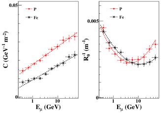
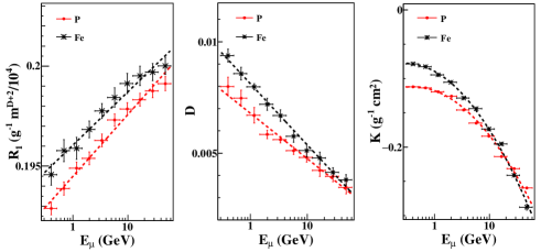
Figure 2: $C$, $R_{0}^{-1}$, $R_{1}$, $D$ and $K$ as a function of $E_{\mu}$. $E_{p}$ = 10¹⁶ eV, $\theta_{p}~{}=~{}0^{\circ}~{}\pm~{}2.5^{\circ}$

In figure 3, the muon density maps of two reconstructed showers initiated by proton and Iron primaries respectively, using Eqn. (3.1) are shown. The value of the $X_{max}$ for the two showers are very close to each other.

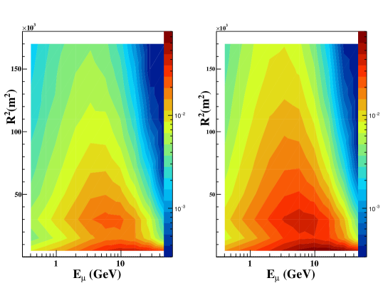
Figure 3: Reconstruction of the shower profile using $\rho_{ER^{2}}$ (GeV^-1 m^-2) for two primaries at $E_{p}~{}=~{}10^{17}$ eV, $\theta_{p}~{}=~{}0^{\circ}~{}\pm~{}2.5^{\circ}$. (Left) Proton initiated shower with $X_{max}$ = 621 g cm^-2, (Right) Fe initiated shower with $X_{max}$ = 620 g cm^-2.

3.2 Parametrization of the lateral muon profile for different primary mass

The number density of muons and the lateral muon profile are then employed to track the primary–type using a basic likelihood test for differentiating between hypotheses. A likelihood function has been constructed using these two components,

$$\ln L=\ln L_{shape}+\ln L_{n},$$ (3.2)

where

$$L_{shape}=\prod_{i=1}^{N_{\mu}^{obs}}\rho_{ER^{2}}^{{}^{\prime}i}(E_{\mu}^{i},R^{i})$$ (3.3)

and

$$L_{n}=Poisson(N_{\mu}^{obs}|N_{\mu}^{exp})$$ (3.4)

Here, $\rho_{ER^{2}}^{{}^{\prime}i}$ is the normalized value of $\rho_{ER^{2}}^{i}$ for the $i^{th}$ muon, $N_{\mu}^{obs}$ is the number of muons observed in an air shower, and $N_{\mu}^{exp}$ is the expected number of muons which is calculated by integrating $\rho_{ER^{2}}$. Now a simple likelihood using the shape profiles from the models of Proton and Fe, and the deviation of the data of a shower from this average profile, gives us important discrimination between the primaries.

We define

$$\Lambda=\ln L(\rm M1)-\ln L(\rm M2)~{}~{}~{}~{}~{}~{}~{}~{}~{}~{}~{}~{}~{}~{}~{}~{}~{}~{}~{}~{}~{}~{}~{}~{}~{}~{}~{}~{}~{}~{}~{}~{}$$ (3.5)

=$\ln L_{shape}(M1)+\ln L_{n}(M1)-\ln L_{shape}(M2)-\ln L_{n}(M2)$

=$\ln L_{shape}(M1)-\ln L_{shape}(M2)+\ln L_{n}(M1)-\ln L_{n}(M2)$

= $\Lambda_{shape}+\Lambda_{n}$.
Here, M1 and M2 refer to two different primary types. The muon profiles $f_{s}$ for M1 and M2 are calculated using appropriate values of $C_{i}^{j}$. The number densities of the muons vary with different primary parameters, due to the difference in the interaction.

4 Results

In this section we discuss the results of the analysis described in section 3.2. We show the potential of the likelihood parameter $\Lambda$ in discriminating between showers from P and Fe primaries. Note that $\Lambda$ has two components $\Lambda_{shape}$ and $\Lambda_{n}$, which correspond to the contributions from the difference in the shower profile shape and the number of muons respectively. We study, with some chosen parameters of the primary particle, the effect of these two components for a number of detection choices.

4.1 P and Fe primaries

We start with an array of ideal 2m $\times$ 2m muon detectors. In an actual surface array, only a small fraction of the air shower secondaries are expected to get detected. We consider four arrangements of the detector stations: the ideal situation of continuous detectors with no gaps between the stations, detector stations 20m apart (a collection of 1% of the secondary muons), detector stations 50m apart (a collection of 0.16% of the secondary muons) and detector stations 200m apart (a collection of 0.01% of the secondary muons). The last two arrangements are close to a realistic array arrangements. We simulate 100 showers from each of the primary particle at a given energy. In order to have a significant statistics in a reasonable computation time, each of the showers is translated a number of times through the detector array at varying positions with respect to the shower core, and each of them are considered a new shower.

The $\Lambda_{shape}$ distributions for two sets of air showers from P and Fe primaries respectively are shown in figure 4. For 100% collection efficiency the two distributions are significantly apart, raising interest to probe further at realistic collections at the detector. A collection of 1% of the entire muons with detector stations 20 m away from one another shows a distinction capability of more than 95% for the two primaries. A more realistic case of 0.16% collection from a detector array with 50 m spacings indicates that the primary detection is possible with more than 50% confidence. An array with 200 m spacing between stations shows rather marginal separation.

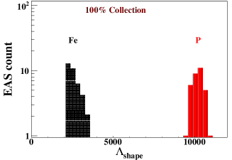
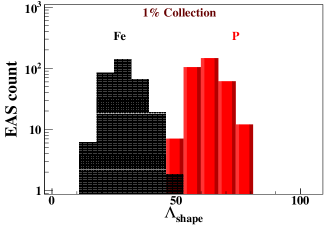
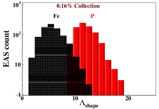
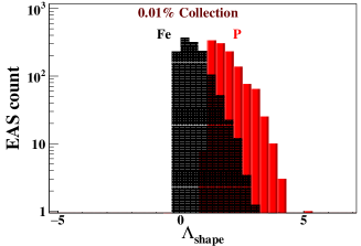
Figure 4: The distributions of $\Lambda_{shape}$ for P and Fe primaries ($E_{p}~{}=~{}10^{16}$ eV, $\theta_{p}~{}=~{}0^{\circ}~{}\pm~{}2.5^{\circ}$) at four different collection efficiencies in an array of simulated 2m $\times$ 2m ideal muon detectors. (Top–left) 100% collection, i.e., no gap between the detectors; (top–right) 1% collection, i.e., detectors 20m apart; (bottom–left) 0.16% collection, i.e., detectors 50m apart; (bottom–right) 0.01% collection, i.e., detectors 200m apart.

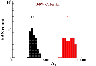
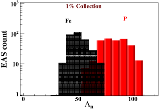
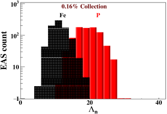
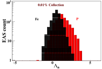
Figure 5: The distributions of $\Lambda_{n}$ for P and Fe primaries ($E_{p}~{}=~{}10^{16}$ eV, $\theta_{p}~{}=~{}0^{\circ}~{}\pm~{}2.5^{\circ}$) at four different collection efficiencies in an array of simulated 2m $\times$ 2m ideal muon detectors. (Top–left) 100% collection, i.e., no gap between the detectors; (Top–right) 1% collection, i.e., detectors 20m apart; (bottom–left) 0.16% collection, i.e., detectors 50m apart; (bottom–right) 0.01% collection, i.e., detectors 200m apart.

The distributions of $\Lambda_{n}$ for the same sets of air showers are shown in figure 5. For the ideal 100% collection efficiency, the two distributions are again wide apart. For detector stations 20 m apart (1% collection), the two primaries can be identified with about 75% confidence. For 0.16% collection, the separation capability is slightly less than 50%. For 0.1% collection, the identification capability is marginal. The two parameters ($\Lambda_{shape}$ and $\Lambda_{n}$) together will enhance the primary identification capability. In figure 6 the projection of the parameters on the two dimensional $\Lambda_{shape}$ – $\Lambda_{n}$ plane are shown. Confidence level contours at three different confidence levels (50%, 90% and 99%) are drawn for air showers from both P and Fe primaries.

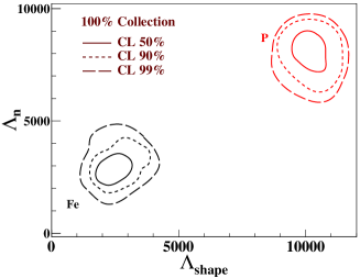
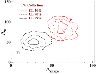
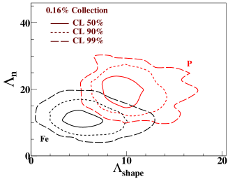
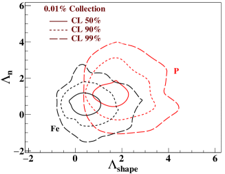
Figure 6: Contours at 50%, 90% and 99% confidence levels in $\Lambda_{shape}$ – $\Lambda_{n}$ plane for P and Fe showers ($E_{p}~{}=~{}10^{16}$ eV, $\theta_{p}~{}=~{}0^{\circ}~{}\pm~{}2.5^{\circ}$) for different collection efficiencies in an array of simulated 2m $\times$ 2m ideal muon detectors. (Top–left) 100% collection, i.e., no gap between the detectors; (Top–right) 1% collection, i.e., detectors 20m apart; (bottom–left) 0.16% collection, i.e., detectors 50m apart; (bottom–right) 0.01% collection, i.e., detectors 200m apart.

In figure. 7, we show the confidence level contours for air showers generated from different primary energies. A rectangular array of 2m $\times$ 2m ideal muon detector stations situated 50 m apart from each other, which implies a collection efficiency of 0.16% is considered here. As the primary energy increases, the number of muons increases and the shape of the muon distributions on $E_{\mu}$ – R plane can be expressed through the density functions $\rho_{ER}$ with lesser uncertainty. This improves the identification of the primary mass through $\Lambda_{shape}$ and $\Lambda_{n}$, which is clear from figure. 7.

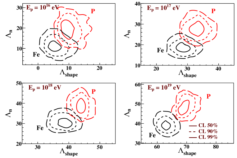
Figure 7: Contours at 50%, 90% and 99% confidence levels in $\Lambda_{shape}$ – $\Lambda_{n}$ plane for P and Fe showers ($\theta_{p}~{}=~{}0^{\circ}~{}\pm~{}2.5^{\circ}$) at various energies of the primary. (Top–right) $E_{p}~{}=~{}10^{16}$ eV; (top–left) $E_{p}~{}=~{}10^{17}$ e; (bottom–right) $E_{p}~{}=~{}10^{18}$ eV, (bottom–left) $E_{p}~{}=~{}10^{19}$ eV. An array of 2m $\times$ 2m ideal muon detectors is considered with collection efficiency 0.16%.

4.2 Incorporating $E_{\mu}$ resolution

All the results so far have been obtained for ideal muon detectors. We now add realistic detector resolution to $E_{\mu}$ which is crucial to design a suitable muon detector. Figure 8 shows the 90% contours for four choices of the $E_{\mu}$ resolutions as listed in table 2, which are added as Gaussian smearing to the true values of $E_{\mu}$. The choice $\sigma_{2}$, which includes a finer resolution for $E_{\mu}~{}\leq$ 10 GeV, shows marginal improvement. At the detector surface level, the muon energy spectrum peaks at a lower energy (<2 GeV) indicating that the low energy region is the most sensitive region for the analysis with muon number and lateral shape.

$\sigma_{1}$	50%
$\sigma_{2}$	20%, $E_{\mu}~{}\leq$ 10 GeV
	50%, $E_{\mu}~{}\textless$ 10 GeV
$\sigma_{3}$	20%, 10 Gev $\leq E_{\mu}~{}\leq$ 20 GeV
	50%, $E_{\mu}~{}\textless$ 10 GeV & $E_{\mu}~{}\textgreater$ 20 GeV
$\sigma_{4}$	20%, $E_{\mu}~{}\geq$ 20 GeV
	50%, $E_{\mu}~{}\textless$ 20 GeV

Table 2: The choices of $\sigma_{E_{\mu}}$

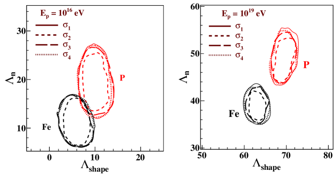
Figure 8: Contours at 90% confidence level in $\Lambda_{shape}$ – $\Lambda_{n}$ plane for P and Fe primaries ($\theta_{p}~{}=~{}0^{\circ}~{}\pm~{}2.5^{\circ}$), at four different choices of $\sigma_{E_{\mu}}$ of the detectors, as detailed in table (2). (Left) $E_{p}$ = $10^{16}eV$, (right) $E_{p}$ = $10^{19}eV$. An array of 2m $\times$ 2m muon detectors is considered with collection efficiency 0.16%

4.3 More primary species

We now extend the analysis to a wide range of primary species. The air showers under study are distributed into three groups according to the mass number of their primaries as shown in Table 1. We use 200 air showers in each group, distributed evenly among the primaries. We denote $M_{I}$, $M_{II}$ and $M_{III}$ to be the corresponding shower profile models of Group I, Group II and Group III respectively. We obtain the following distinguishing parameters from the log–likelihood study.

$$\Lambda(k)=\ln~{}L(M_{k})~{}-~{}\ln~{}L(M_{III});~{}\rm{where}~{}k=I,II,III$$ (4.1)

In figure 9, the $\Lambda_{shape}$ – $\Lambda_{n}$ 2-dimensional contours are drawn for the three groups for the most ideal case of 100% collection with ideal muon detectors.

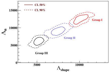
Figure 9: Contours at 50% and 90% confidence levels in $\Lambda_{shape}$ – $\Lambda_{n}$ plane for three groups of primary chosen on the basis of primary mass. Here, $E_{p}~{}=~{}10^{16}$ eV and $\theta_{p}~{}=~{}0^{\circ}~{}\pm~{}2.5^{\circ}$. An array of 2m $\times$ 2m ideal muon detectors is considered with collection efficiency 100%.

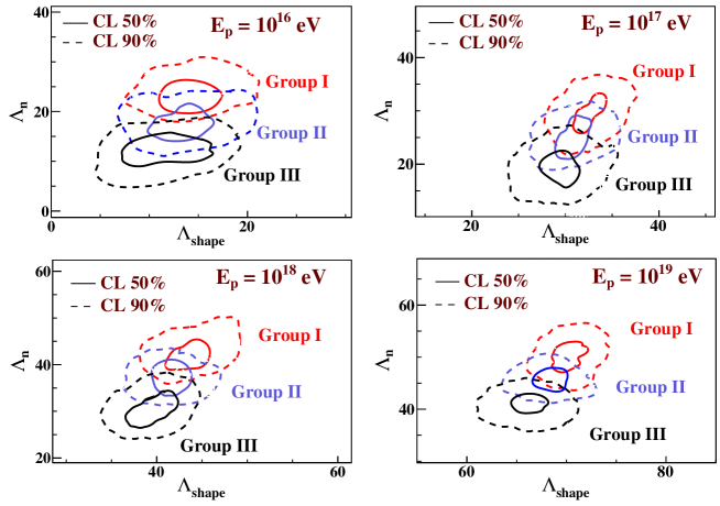
Figure 10: Contours at 50% and 90% confidence levels in $\Lambda_{shape}$ – $\Lambda_{n}$ plane for three groups of primary ($\theta_{p}~{}=~{}0^{\circ}~{}\pm~{}2.5^{\circ}$) chosen on the basis of primary mass. (Top–right) $E_{p}~{}=~{}10^{16}$ eV; (top–left) $E_{p}~{}=~{}10^{17}$ eV; (bottom–right) $E_{p}~{}=~{}10^{18}$ eV, (bottom–left) $E_{p}~{}=~{}10^{19}$ eV. An array of 2m $\times$ 2m muon detectors ($\sigma_{E_{\mu}}$ = 20% for $E_{\mu}~{}\textless~{}10$ GeV, $\sigma_{E_{\mu}}$ = 50% for $E_{\mu}~{}\textgreater~{}10$ GeV) is considered with collection efficiency 0.16% .

We then probe further with 0.16% collection. Figure 10 shows the results at 0.16% collection for showers at various energy of the primary in the range $10^{16}$ eV – $10^{19}$ eV and realistic detector energy resolution.

4.4 Hadron models

The very high energy hadronic interactions are not well understood yet and are a major source of uncertainty in our analysis as well as other analyses in the field. The previous results use the interaction model QGSJET II–04. Here we probe the fluctuations arising from three different hadron interaction models: QGSJET II–04, EPOS LHC and SIBYLL, used to simulate the high energy interactions. Figure 11 compares the 90% confidence level contours for these three interaction models for air showers generated from P and Fe primaries. It can be easily seen that SIBYLL predicted shapes and numbers are significantly away from the other two models which in turn agree quite well with each other.

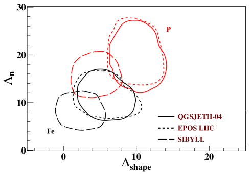
Figure 11: Contours at 90% confidence level in $\Lambda_{shape}$ – $\Lambda_{n}$ plane for P and Fe primaries, for showers generated with three high energy interaction models QGSJETII-04, EPOS LHC and SIBYLL. Here, $E_{p}$ = $10^{16}$ eV and $\theta_{p}~{}=~{}0^{\circ}~{}\pm~{}2.5^{\circ}$. An array of 2m $\times$ 2m muon detectors ($\sigma_{E_{\mu}}$ = 20% for $E_{\mu}~{}\textless~{}10$ GeV, $\sigma_{E_{\mu}}$ = 50% for $E_{\mu}~{}\textgreater~{}10$ GeV) is considered with collection efficiency 0.16%.

5 Summary and future prospects

In this study, we performed a simulation study using CORSIKA to combine the longitudinal profile of the muons, characterized by their energy spectrum and lateral spread, with the depth at shower maximum ($X_{max}$) of an EAS initiated by a primary at ultra high energies ($10^{16}$ eV – $10^{19}$ eV). Firstly, using proton and iron as the shower primaries, we show that the muon observables and $X_{max}$ together can be used to identify the primary with relatively high acceptance and confidence. We find that for 0.16% muon collection using a detector array of 2m $\times$ 2m detectors 50m apart from each other, we can distinguish P and Fe primaries at an acceptance above 50%. This study is then generalized with three groups of primaries light, medium and heavy. The hadronic interaction models at higher energies are a major source of uncertainties, and we find a significant deviation among the models tested in this study. This deviation can also be a tool to probe the models at the UHE region using cosmic air shower data.

The simulation involved 2m $\times$ 2m detector stations for muon detection. We find that a muon detector which is more sensitive to lower energies ($E_{\mu}\textless 10$ GeV) improves the results. We will extend this study to detailed analysis of different interaction models. We plan to build a prototype surface station of such dimensions based on a scalable and economic technology, which would be sensitive to individual muons events and will be able to measure their energies and direction.

6 Acknowledgements

The authors thank the Weizmann Institute and Yeda-Sela foundation for the generous support. This work was supported by a Pazy-Vatat grant for young scientists. RB is the incumbent of the Arye and Ido Dissentshik Career Development Chair. The authors also thank Dr. Hagar Landsman, Dr. Lorne Levinson, Dr. Alessandro Manfredini and Mr. Nadav Priel for the discussions in the course of this work.

References

- [1] K. Greisen, End to the cosmic ray spectrum?, Phys. Rev. Lett. 16 (1966) 748–750.
- [2] G. T. Zatsepin and V. A. Kuzmin, Upper limit of the spectrum of cosmic rays, JETP Lett. 4 (1966) 78–80. [Pisma Zh. Eksp. Teor. Fiz.4,114(1966)].
- [3] A. M. Hillas, Cosmic Rays: Recent Progress and some Current Questions, in Conference on Cosmology, Galaxy Formation and Astro-Particle Physics on the Pathway to the SKA Oxford, England, April 10-12, 2006, 2006. astro-ph/0607109.
- [4] D. De Marco and T. Stanev, On the shape of the UHE cosmic ray spectrum, Phys. Rev. D72 (2005) 081301, [astro-ph/0506318].
- [5] E. Waxman, Gamma-ray bursts, cosmic rays and neutrinos, Nucl. Phys. Proc. Suppl. 87 (2000) 345–354, [astro-ph/0002243].
- [6] D. Maurin, F. Melot, and R. Taillet, A database of charged cosmic rays, Astron. Astrophys. 569 (2014) A32, [arXiv:1302.5525].
- [7] B. M. and B. V. et al., The cosmic-ray proton and helium spectra measured with the {CAPRICE98} balloon experiment, Astroparticle Physics 19 (2003), no. 5 583 – 604.
- [8] Cosmic protons, Physics Letters B 490 (2000), no. 1–2 27 – 35.
- [9] Helium in near earth orbit, Physics Letters B 494 (2000), no. 3–4 193 – 202.
- [10] T. Sanuki and M. M. et. al., Precise measurement of cosmic-ray proton and helium spectra with the bess spectrometer, The Astrophysical Journal 545 no. 2 1135.
- [11] Measurements of primary and atmospheric cosmic-ray spectra with the bess-tev spectrometer, Physics Letters B 594 (2004), no. 1–2 35 – 46.
- [12] M. Ave, P. J. Boyle, F. Gahbauer, C. Hoppner, J. R. Horandel, M. Ichimura, D. Muller, and A. Romero-Wolf, Composition of Primary Cosmic-Ray Nuclei at High Energies, Astrophys. J. 678 (2008) 262, [arXiv:0801.0582].
- [13] A. Panov, N. Sokolskaya, and V. Zatsepin, Upturn in the ratio of nuclei of to iron observed in the {ATIC} experiment and the local bubble, Nuclear Physics B - Proceedings Supplements 256–257 (2014) 233 – 240. Cosmic Ray Origin – Beyond the Standard Models.
- [14] V. A. Derbina, V. I. Galkin, and et al., Cosmic-ray spectra and composition in the energy range of 10-1000 tev per particle obtained by the runjob experiment, The Astrophysical Journal Letters 628 no. 1 L41.
- [15] K. Asakimori, T. H. Burnett, and et al., Cosmic-ray proton and helium spectra: Results from the jacee experiment, The Astrophysical Journal 502 no. 1 278.
- [16] Pierre Auger Collaboration, A. Aab et al., Depth of maximum of air-shower profiles at the Pierre Auger Observatory. II. Composition implications, Phys. Rev. D90 (2014), no. 12 122006, [arXiv:1409.5083].
- [17] Pierre Auger Collaboration, A. Aab et al., Depth of maximum of air-shower profiles at the Pierre Auger Observatory. I. Measurements at energies above eV, Phys. Rev. D90 (2014), no. 12 122005, [arXiv:1409.4809].
- [18] Pierre Auger, Telescope Array Collaboration, R. U. Abbasi et al., Pierre Auger Observatory and Telescope Array: Joint Contributions to the 34th International Cosmic Ray Conference (ICRC 2015), arXiv:1511.0210.
- [19] Pierre Auger Collaboration, A. Aab et al., Evidence for a mixed mass composition at the ‘ankle’ in the cosmic-ray spectrum, Phys. Lett. B762 (2016) 288–295, [arXiv:1609.0856].
- [20] Pierre Auger Collaboration, A. Aab et al., Measurement of the cosmic ray spectrum above 4 1018 eV using inclined events detected with the Pierre Auger Observatory, JCAP 1508 (2015) 049, [arXiv:1503.0778].
- [21] T. Fujii, The Mass Composition of Ultra-high Energy Cosmic Rays Measured by New Fluorescence Detectors in the Telescope Array Experiment, Physics Procedia 61 (2015) 418–424. 13th International Conference on Topics in Astroparticle and Underground Physics, TAUP 2013.
- [22] P. Tinyakov, Latest results from the telescope array, Nuclear Instruments and Methods in Physics Research Section A: Accelerators, Spectrometers, Detectors and Associated Equipment 742 (2014) 29 – 34. 4th Roma International Conference on Astroparticle Physics.
- [23] R. U. Abbasi et al., Study of Ultra-High Energy Cosmic Ray composition using Telescope Array’s Middle Drum detector and surface array in hybrid mode, Astropart. Phys. 64 (2015) 49–62, [arXiv:1408.1726].
- [24] Telescope Array Collaboration, T. Abu-Zayyad et al., Energy Spectrum of Ultra-High Energy Cosmic Rays Observed with the Telescope Array Using a Hybrid Technique, Astropart. Phys. 61 (2015) 93–101, [arXiv:1305.7273].
- [25] R. U. Abbasi et al., Search for EeV Protons of Galactic Origin, Astropart. Phys. 86 (2017) 21–26, [arXiv:1608.0630].
- [26] Pierre Auger Collaboration, J. Abraham et al., Measurement of the energy spectrum of cosmic rays above eV using the Pierre Auger Observatory, Phys. Lett. B685 (2010) 239–246, [arXiv:1002.1975].
- [27] HiRes Collaboration, R. U. Abbasi et al., Indications of proton-dominated cosmic ray composition above 1.6 eev, Phys. Rev. Lett. 104 (2010) 161101, [arXiv:0910.4184].
- [28] R. Aloisio, V. Berezinsky, and P. Blasi, Ultra high energy cosmic rays: implications of Auger data for source spectra and chemical composition, JCAP 1410 (2014), no. 10 020, [arXiv:1312.7459].
- [29] R.-Y. Liu, A. M. Taylor, M. Lemoine, X.-Y. Wang, and E. Waxman, Constraints on the Source of Ultra-high-energy Cosmic Rays Using Anisotropy versus Chemical Composition, Astrophys. J. 776 (2013) 88, [arXiv:1308.5699].
- [30] A. Strong, I. Moskalenko, and P. V.S., Cosmic-ray propagation and interactions in the galaxy, Annu. Rev. Nucl. Part. Sci 57 (2007) 285–327.
- [31] A. A. Abdo et al., The Large Scale Cosmic-Ray Anisotropy as Observed with Milagro, Astrophys. J. 698 (2009) 2121–2130, [arXiv:0806.2293].
- [32] Fermi LAT Collaboration Collaboration, A. A. Abdo, M. Ackermann, and et al., Measurement of the cosmic ray spectrum from 20 gev to 1 tev with the fermi large area telescope, Phys. Rev. Lett. 102 (May, 2009) 181101.
- [33] Fermi LAT Collaboration Collaboration, M. Ackermann, M. Ajello, and et al., Fermi lat observations of cosmic-ray electrons from 7 gev to 1 tev, Phys. Rev. D 82 (Nov, 2010) 092004.
- [34] AMS Collaboration Collaboration, M. Aguilar, D. Aisa, and et al., Precision measurement of the flux in primary cosmic rays from 0.5 gev to 1 tev with the alpha magnetic spectrometer on the international space station, Phys. Rev. Lett. 113 (Nov, 2014) 221102.
- [35] H.E.S.S. Collaboration Collaboration, F. Aharonian, A. G. Akhperjanian, and et al., Energy spectrum of cosmic-ray electrons at tev energies, Phys. Rev. Lett. 101 (Dec, 2008) 261104.
- [36] O. Adriani, G. C. Barbarino, and et al., Cosmic-ray electron flux measured by the pamela experiment between 1 and 625 gev, Phys. Rev. Lett. 106 (May, 2011) 201101.
- [37] R. Abbasi, Y. Abdou, T. Abu-Zayyad, J. Adams, J. A. Aguilar, M. Ahlers, K. Andeen, J. Auffenberg, X. Bai, M. Baker, and t. . et al.
- [38] J. Chang, A. J. H., and et al., An excess of cosmic ray electrons at energies of 300-800GeV, nature 456 (Nov., 2008) 362–365.
- [39] E. Bugaev et al., Cosmic muons and neutrinos, Moscow: Atomizd.
- [40] T. K. Gaisser, Cosmic Rays And Particle Physics. Cambridge University Press, 1990.
- [41] K. Greisen, Cosmic ray showers, Annual Review of Nuclear Science.
- [42] T. Nonaka, M. Takamura, K. Honda, J. N. Matthews, S. Ogio, N. Sakurai, H. Sagawa, B. T. Stokes, M. Tsujimoto, and K. Yashiro, Muon Detector R&D in Telescope Array Experiment. http://journals.jps.jp/doi/pdf/10.7566/JPSCP.9.010013.
- [43] Pierre Auger Collaboration, A. Aab et al., Muon counting using silicon photomultipliers in the AMIGA detector of the Pierre Auger observatory, JINST 12 (2017), no. 03 P03002, [arXiv:1703.0619].
- [44] A. Breskin et al., CsI-THGEM gaseous photomultipliers for RICH and noble-liquid detectors, Nucl. Instrum. Meth. A639 (2011) 117–120, [arXiv:1009.5883].
- [45] A. Rubin, L. Arazi, S. Bressler, L. Moleri, M. Pitt, and A. Breskin, First studies with the Resistive-Plate WELL gaseous multiplier, JINST 8 (2013) P11004, [arXiv:1308.6152].
- [46] L. Moleri et al., In-beam evaluation of a medium-size Resistive-Plate WELL gaseous particle detector, JINST 11 (2016), no. 09 P09013, [arXiv:1607.0258].
- [47] R. Santonico and R. Cardarelli, Development of resistive plate counters, Nuclear Instruments and Methods in Physics Research 187 (1981), no. 2 377 – 380.
- [48] D. Heck, J. Knapp, J. N. Capdevielle, G. Schatz, and T. Thouw, CORSIKA: a Monte Carlo code to simulate extensive air showers. Feb., 1998.
- [49] J. Ranft, Dual parton model at cosmic ray energies, Phys. Rev. D 51 (Jan, 1995) 64–84.
- [50] N. N. Kalmykov and S. S. Ostapchenko, The Nucleus-nucleus interaction, nuclear fragmentation, and fluctuations of extensive air showers, Phys. Atom. Nucl. 56 (1993) 346–353. [Yad. Fiz.56N3,105(1993)].
- [51] N. N. Kalmykov, S. S. Ostapchenko, and A. I. Pavlov, EAS and a quark - gluon string model with jets, Bull. Russ. Acad. Sci. Phys. 58 (1994) 1966–1969. [Izv. Ross. Akad. Nauk Ser. Fiz.58N12,21(1994)].
- [52] R. S. Fletcher, T. K. Gaisser, P. Lipari, and T. Stanev, SIBYLL: An Event generator for simulation of high-energy cosmic ray cascades, Phys. Rev. D50 (1994) 5710–5731.
- [53] J. Engel, T. K. Gaisser, T. Stanev, and P. Lipari, Nucleus-nucleus collisions and interpretation of cosmic ray cascades, Phys. Rev. D46 (1992) 5013–5025.
- [54] K. Werner, Strings, pomerons, and the venus model of hadronic interactions at ultrarelativistic energies, Phys. Rept. 232 (1993) 87–299.
- [55] H. Drescher, M. Hladik, S. Ostapchenko, T. Pierog, and K. Werner, Parton-based gribov–regge theory, Physics Reports 350 (2001), no. 2 93 – 289.
- [56] T. Pierog, I. Karpenko, J. M. Katzy, E. Yatsenko, and K. Werner, EPOS LHC: Test of collective hadronization with data measured at the CERN Large Hadron Collider, Phys. Rev. C92 (2015), no. 3 034906, [arXiv:1306.0121].
- [57] S. Ostapchenko, Monte carlo treatment of hadronic interactions in enhanced pomeron scheme: Qgsjet-ii model, Phys. Rev. D 83 (Jan, 2011) 014018.
- [58] S. Ostapchenko, Qgsjet-ii: towards reliable description of very high energy hadronic interactions, Nuclear Physics B - Proceedings Supplements 151 (2006), no. 1 143 – 146. VERY HIGH ENERGY COSMIC RAY INTERACTIONS.
- [59] A. Fasso et al., The Physics models of FLUKA: Status and recent developments, eConf C0303241 (2003) MOMT005, [hep-ph/0306267].
- [60] H. Fesefeldt, The simulation of hadron showers, RWTH Aachen Report 51 (Jan, 1995) 64–84.
- [61] S. A. Bass et al., Microscopic models for ultrarelativistic heavy ion collisions, Prog. Part. Nucl. Phys. 41 (1998) 255–369, [nucl-th/9803035]. [Prog. Part. Nucl. Phys.41,225(1998)].