Dynamical gap generation in 2D Dirac semimetal with deformed Dirac cone

Abstract

According to the extensive theoretical and experimental investigations, it is widely accepted that the long-range Coulomb interaction is too weak to generate a dynamical excitonic gap in graphene with a perfect Dirac cone. We study the impact of the deformation of Dirac cone on dynamical gap generation. When a uniaxial strain is applied to graphene, the Dirac cone is made elliptical in the equal-energy plane and the fermion velocity becomes anisotropic. The applied uniaxial strain has two effects: it decreases the fermion velocity; it increases the velocity anisotropy. After solving the Dyson-Schwinger gap equation, we show that dynamical gap generation is promoted by the former effect, but is suppressed by the latter one. For suspended graphene, we find that the systems undergoes an excitonic insulating transition when the strain is roughly 7.34$\%$. We also solve the gap equation in case the Dirac cone is tiled, which might be realized in the organic material $\alpha$-(BEDT-TTF)₂I₃, and find that the tilt of Dirac cone can suppress dynamical gap generation. It turns out that the geometry of the Dirac cone plays an important role in the formation of excitonic pairing.

I INTRODUCTION

Semimetals, no matter topologically trivial or non-trivial, have attracted intensive theoretical and experimental studies because of their intriguing properties and promising industrial applications Vafek14 ; Wehling14 ; Weng16 ; Yan17 ; Hasan17 . Among all known semimetals, two-dimensional (2D) Dirac semimetal plays a special role. There are two famous examples for such semimetals: graphene CastroNeto09 ; Kotov12 ; surface state of three-dimensional (3D) topological insulator (TI) Hasan10 ; Qi11 . The low-energy excitations of these systems are massless Dirac fermions, described by the relativistic Dirac equation.

In contrast to normal metals that possess a finite Fermi surface, the Fermi surface of 2D Dirac semimetal shrinks to a number of discrete points at which the valence and conduction bands touch CastroNeto09 ; Kotov12 . The Coulomb interaction between Dirac fermions remains long-ranged since the density of states (DOS) vanishes at the Fermi level. The influences of long-range Coulomb interaction on the low-energy dynamics of Dirac fermions has been extensively investigated Kotov12 . Although weak Coulomb interaction is found by renormalization group (RG) analysis to be marginally irrelevant Shankar94 ; Gonzalez94 ; Gonzalez99 ; Son07 ; Hofmann14 ; Bauer15 ; Sharma16 , it gives rise to singular renormalization of fermion velocity Gonzalez94 ; Gonzalez99 ; Son07 ; Hofmann14 ; Bauer15 ; Sharma16 and logarithmic-like corrections to a variety of observable quantities, including specific heat, optical conductivity, thermal conductivity, and compressibility etc Kotov12 . The singular renormalization of fermion velocity has been experimentally confirmed in suspended graphene Elias11 , quasi-freestanding graphene on silicon carbide (SiC) Siegel11 , and graphene on boron nitride substrate Yu13 .

The Coulomb interaction can also induce important non-perturbative effects. Of particular interest is the possibility of semimetal-insulator quantum phase transition driven by the dynamical generation of a finite excitonic gap Khveshchenko01 ; CastroNetoPhysics09 ; Gorbar02 ; Khveshchenko04 ; Liu09 ; Khveshchenko09 ; Gamayun10 ; Sabio10 ; Zhang11 ; Liu11 ; WangLiu11A ; WangLiu11B ; WangLiu12 ; Popovici13 ; WangLiu14 ; Gonzalez15 ; Carrington16 ; Gamayun09 ; WangJianhui11 ; Katanin16 ; Vafek08 ; Gonzalez10 ; Gonzalez12 ; Drut09A ; Drut09B ; Drut09C ; Armour10 ; Armour11 ; Buividovich12 ; Ulybyshev13 ; Smith14 ; Juan12 ; Kotikov16 . Once an excitonic gap is opened, the chiral symmetry, corresponding to symmetry of sublattices, is dynamically broken Kotov12 ; Khveshchenko01 . The research interest in dynamical gap generation is twofold. Firstly, acquiring a finite gap broadens the possible applications of graphene in the design and manufacture of electronic devices CastroNetoPhysics09 . Secondly, it is the condensed-matter counterpart of the concept of dynamical chiral symmetry breaking Nambu61 ; Miransky .

Several years before monolayer graphene was isolated in laboratory, Khveshchenko Khveshchenko01 discussed the possibility of dynamical gap generation for massless Dirac fermions in 2D, motivated by the theoretical progress of dynamical chiral symmetry breaking in (2+1)-dimensional QED. His main result Khveshchenko01 is that a finite excitonic gap can be generated if the Coulomb interaction strength $\alpha$, defined by

$$\alpha=\frac{e^{2}}{v\kappa},$$ (1)

where $e$ is the electric charge, $v$ fermion velocity, and $\kappa$ dielectric constant, is larger than some threshold $\alpha_{c}$ for a fixed fermion flavor $N_{f}$. This interesting result has stimulated extensive theoretic and numerical studies aimed at finding the precise value of $\alpha_{c}$. Calculations performed by Dyson-Schwinger (DS) equation Khveshchenko04 ; Liu09 ; Khveshchenko09 ; Gamayun10 ; Zhang11 ; WangLiu11A , Bethe-Slapeter (BS) equation Gamayun09 ; WangJianhui11 , RG approach Vafek08 ; Gonzalez12 , and Monte Carlo simulation Drut09A ; Drut09B found that the critical value $\alpha_{c}$ falls into the range $0.79<\alpha_{c}<2.16$. For suspended graphene, the interaction strength is $\alpha\approx 2.16$, whereas for graphene placed on SiO₂ substrate, it becomes $\alpha\approx 0.79$ CastroNetoPhysics09 . It thus indicates that suspended graphene is an excitonic insulator at zero $T$, but graphene placed on SiO₂ remains a semimetal. However, experiments did not find any evidence for the existence of excitonic insulating phase in suspended graphene even at very low temperatures Elias11 ; Mayorov12 . In Ref.WangLiu12 , the authors studied the DS equation for excitonic gap by incorporating the wave function renormalization, fermion velocity renormalization, and dynamical gap generation in an unbiased way, and found that $\alpha_{c}\sim 3.2$ WangLiu12 . According to this result, the Coulomb interaction in suspended graphene is too weak to drive the semimetal-insulator phase transition. This conclusion is well consistent with experiments Mayorov12 , and is also confirmed by subsequent more refined DS equation studies Gonzalez15 ; Carrington16 . In addition, recent Monte Carlo simulations Ulybyshev13 ; Smith14 claimed that, although the Coulomb interaction in suspended graphene is not strong enough to open an excitonic gap, the $\alpha_{c}$ is close to $2.16$.

Although careful experiments and elaborate theoretical studies have already provided strong evidences for the absence of excitonic gap in intrinsic graphene, there have been several proposals attempting to realize excitonic insulator in similar semimetals. For example, it was argued that the Coulomb interaction in an organic material $\alpha$-(BEDT-TTF)₂I₃ might be much stronger than graphene, because its fermion velocity is about one-tenth of the one observed in graphene Monteverde13 . In addition, Triola et al. proposed that the fermion excitations of surface state of some topological Kondo insulators may have extraordinary small fermion velocities, which would drive the Coulomb interaction to fall into the strong coupling regime Triola15 . Moreover, it seems viable to strengthen the Coulomb interaction and as such promote excitonic insulating transition by exerting certain extrinsic influences. Through Monte Carlo simulations, Tang et al. argued that applying a uniform and isotropic strain by about 15$\%$ can make the Coulomb interaction strong enough to open an excitonic gap Tang15 .

Recently, the influence of a uniaxial strain on the properties of Dirac fermions has been studied. First principle calculations Pereira09 ; Choi10 suggested that the uniaxial strain would cause the carbon-carbon bond become longer along the direction of the applied strain and get shorter along its orthogonal direction. As a consequence, the originally perfect Dirac cone is deformed, and the fermion velocity along the direction of applied uniaxial strain decreases, whereas the other component of fermion velocity is made larger. Sharma et al. Sharma17 investigated the possibility of dynamical gap generation in graphene with an anisotropic dispersion, and argued that it is promoted by the velocity anisotropy induced by the uniaxial strain.

In this paper, we study the influence of uniaxial strain on the formation of excitonic pairing. It is important to emphasize here that applying a uniaxial strain to graphene has two effects: first, it lowers the mean value of fermion velocity; second, it increases the velocity anisotropy. They might have different effects on dynamical gap generation. We will address this issue by solving the self-consistent DS equation for the excitonic gap. We will show that, the two effects of uniaxial strain are actually competitive since they have opposite influences on dynamical gap generation. After carrying out numerical calculations based on three widely adopted approximations, we obtain the dependence of excitonic gap on two parameters, namely the effective Coulomb interaction strength $\alpha=e^{2}/\bar{v}\epsilon$, where $\bar{v}=\sqrt{v_{x}v_{y}}$, and the velocity ratio $\eta=v_{x}/v_{y}$. We will show that the dynamical gap generation is enhanced if the mean value of fermion velocity $\bar{v}$ is lowered, but can be strongly suppressed when the velocity anisotropy grows. Our conclusion is qualitatively consistent with Ref. WangLiu14 . We will present a comparison between our results and that reported in Ref. Sharma17 .

Apart from strain-induced anisotropy Pereira09 ; Choi10 , the fermion velocity anisotropy can also be induced by introducing certain periodic potentials Park08A ; Park08B ; Rusponi10 . Moreover, it is found that the surface state of some topological insulators, including $\beta$-Ag₂Te ZhangWei11 and $\beta$-HgS Virot11 , is 2D Dirac semimetal with two unequal components of fermion velocity. Our results of the impact of velocity anisotropy on dynamical gap generation are applicable to these systems.

To gain more quantitative knowledge of the effects caused by uniaxial strain, we extract an approximated expression for the fermion velocity from recent first-principle calculations of uniaxially strained graphene Choi10 . For suspended graphene, we find that as the applied uniaxial strain grows the system undergoes a semimetal-insulator phase transition when the strain becomes larger than 7.34$\%$. The dependence of dynamical gap on the magnitude of uniaxial strain is obtained from the solution of gap equation, which shows that the gap is an increasing function of the applied strain. We thus see that the enhancement of dynamical gap generation caused by the decreasing mean velocity dominates over the suppressing effect produced by the increasing velocity anisotropy.

In addition to the uniaxial strain, the Dirac cone may be deformed in other ways. For instance, the Dirac cone is known to be tilted in an organic material $\alpha$-(BEDT-TTF)₂I₃ Tajima09 ; Isobe12 ; Nishine10 ; Sari14 ; Trescher15 ; Proskurin15 ; Hirata17 , which is regarded as a promising candidate to realize the quantum phase transition from 2D Dirac semimetal to excitonic insulator Monteverde13 . We also study the fate of dynamical gap generation in such systems, and show that it is suppressed when the Dirac cone is tilted.

The rest sections of the paper are organized as follows. In Sec. II, we give the model action for 2D Dirac fermions with anisotropic dispersion. In Sec. III, we derive the DS gap equation, and then solve it by employing three different approximations. The numerical results are presented and discussed in Sec. IV. In Sec. V, we compare our results with a recent work. The direct relation between strain and gap generation is investigated in Sec. VI. The influence of tilted Dirac cone on dynamical gap generation is studied in Sec. VII. We end the paper with a brief summary in Sec. VIII.

II Model and Feynman rules

The massless Dirac fermions with an anisotropic dispersion can be described by the action

$$S = \int dtd^{2}\mathbf{r}\bar{\Psi}_{\sigma}(\mathbf{r})(i\gamma_{0}\partial_{t}-iv_{x}\gamma_{1}\nabla_{x}-iv_{y}\gamma_{2}\nabla_{y})\Psi_{\sigma}(\mathbf{r})$$ (2)

$$-\frac{1}{2}\int dtdt^{\prime}d^{2}\mathbf{r}d^{2}\mathbf{r}^{\prime}\bar{\Psi}_{\sigma 1}(\mathbf{r})\gamma_{0}\Psi_{\sigma 1}(\mathbf{r})$$

$$\times U_{0}(t-t^{\prime},|\mathbf{r}-\mathbf{r}^{\prime}|)\bar{\Psi}_{\sigma 2}(\mathbf{r}^{\prime})\gamma_{0}\Psi_{\sigma 2}(\mathbf{r}^{\prime}).$$

In this action, $\Psi_{\sigma}^{T}=(\Psi_{Ka\sigma},\Psi_{K^{\prime}a\sigma},\Psi_{Kb\sigma},\Psi_{K^{\prime}b\sigma})$ is a four-component spinor field, representing the low-energy Dirac fermion excitations of graphene, where $a$ and $b$ stand for the two inequivalent sublattices, and $K$ and $K^{\prime}$ for two valleys. The fermion flavor $\sigma=1,2,...N_{f}$, corresponding to the spin components. Although the physical flavors is $N_{f}=2$, in the following analysis we will consider a general large $N_{f}$ so as to perform the $1/N_{f}$ expansion. The $\gamma$-matrices are defined as $\gamma_{0,1,2}=(\tau_{3},i\tau_{2},-i\tau_{1})\otimes\tau_{3}$, where $\tau_{1,2,3}$ are the Pauli matrices.

The free fermion propagator

$$G_{0}(i\omega,\textbf{k})=\frac{1}{-i\omega\gamma_{0}+v_{x}k_{x}\gamma_{1}+v_{y}k_{y}\gamma_{2}}.$$ (3)

The bare Coulomb interaction between fermions is

$$\emph{U}_{0}(t,\textbf{r})=\frac{e^{2}\delta(t)}{\kappa|\mathbf{r}|},$$ (4)

where the dielectric constant $\kappa=\epsilon_{r}\epsilon_{0}$. $\epsilon_{0}$ is the dielectric constant in vacuum, and $\epsilon_{r}$ is a parameter determined by substrate. After making a Fourier transformation, we obtain its expression in the momentum space:

$$\emph{U}_{0}(\textbf{q}) = \frac{e^{2}}{\kappa}\int\frac{d^{2}\mathbf{x}}{2\pi}\frac{\exp(-i\mathbf{qr})\delta(t)}{|\mathbf{r}|}$$ (5)

$$= \frac{2\pi e^{2}\delta(t)}{\kappa|\mathbf{q}|}.$$

The bare Coulomb interaction will always be dynamically screened by the collective electron-hole pairs, which is encoded by the polarization function. To the leading order of $1/N_{f}$ expansion, the polarization function is given by

$$\Pi(i\Omega,\textbf{q}) = -N_{f}\int\frac{d\omega}{2\pi}\frac{d^{2}\textbf{k}}{(2\pi)^{2}}\mathrm{Tr}\left[\gamma_{0}G_{0}(i\omega,\textbf{k})\gamma_{0}\right.$$ (6)

$$\left.\times G_{0}(i\omega+i\Omega,\textbf{k}+\textbf{q})\right]$$

$$= \frac{N_{f}}{8v_{x}v_{y}}\frac{v_{x}^{2}q_{x}^{2}+v_{y}^{2}q_{y}^{2}}{\sqrt{\Omega^{2}+v_{x}^{2}q_{x}^{2}+v_{y}^{2}q_{y}^{2}}}.$$

After including this polarization, the dressed Coulomb propagator can be written as

$$D(i\Omega,\mathbf{q})=\frac{1}{\frac{\kappa|\mathbf{q}|}{2\pi e^{2}}+\frac{N_{f}}{8v_{x}v_{y}}\frac{v_{x}^{2}q_{x}^{2}+v_{y}^{2}q_{y}^{2}}{\sqrt{\Omega^{2}+v_{x}^{2}q_{x}^{2}+v_{y}^{2}q_{y}^{2}}}}.$$ (7)

III Dyson-Schwinger equation

In the presence of Coulomb interaction, the dynamics of Dirac fermions will be significantly affected. Generically, the dressed fermion propagator has the form

$$G(i\omega,\mathbf{k})=\frac{1}{-i\omega A_{0}\gamma_{0}+v_{x}k_{x}A_{1}\gamma_{1}+v_{y}k_{y}A_{2}\gamma_{2}+m},$$ (8)

where $A_{0,1,2}\equiv A_{0,1,2}(i\omega,\mathbf{k})$ are the renormalization functions and $m\equiv m(i\omega,\mathbf{k})$ is the dynamical fermion gap. The renormalized and free propagators are connected by the DS equation

$$G^{-1}(i\varepsilon,\mathbf{p}) = G_{0}^{-1}(i\varepsilon,\mathbf{p})+\int\frac{d\omega}{2\pi}\frac{d^{2}\mathbf{k}}{(2\pi)^{2}}\gamma_{0}G(i\omega,\mathbf{k})$$ (9)

$$\times\gamma_{0}\Gamma(i\varepsilon,\mathbf{p};i\omega,\mathbf{k})D(i(\varepsilon-\omega),\mathbf{p}-\mathbf{k}),$$

where $\Gamma(i\varepsilon,\mathbf{p};i\omega,\mathbf{k})$ is the vertex correction. As demonstrated in Refs. WangLiu12 ; Gonzalez15 ; Carrington16 , the functions $A_{0,1,2}(i\omega,\mathbf{k})$ and the vertex $\Gamma(i\varepsilon,\mathbf{p};i\omega,\mathbf{k})$ play an important role in the determination of the precise value of $\alpha_{c}$. The purpose of the present work is to examine whether dynamical gap generation is enhanced or suppressed by the velocity anisotropy. The qualitative impact of anisotropy actually does not rely on the precise value of $\alpha_{c}$. For our purpose, we will retain only the leading order contribution of the $1/N_{f}$ expansion to the DS equation Khveshchenko01 ; Gorbar02 ; Khveshchenko04 ; Liu09 , and set $A_{0}=A_{1}=A_{2}=1$. Under this approximation, the Ward identity requires $\Gamma=1$. Now it is easy to find that the dynamical fermion gap $m(i\varepsilon,p_{x},p_{y})$ satisfies the following nonlinear integral equation:

$$m(i\varepsilon,p_{x},p_{y}) = \int\frac{d\omega}{2\pi}\int\frac{dk_{x}}{2\pi}\int\frac{dk_{y}}{2\pi}\frac{m(i\omega,k_{x},k_{y})}{\omega^{2}+v_{x}^{2}k_{x}^{2}+v_{y}^{2}k_{y}^{2}+m^{2}(i\omega,k_{x},k_{y})}\frac{1}{\frac{|\mathbf{q}|}{\frac{2\pi e^{2}}{\kappa}}+\frac{N_{f}}{8v_{x}v_{y}}\frac{v_{x}^{2}q_{x}^{2}+v_{y}^{2}q_{y}^{2}}{\sqrt{\Omega^{2}+v_{x}^{2}q_{x}^{2}+v_{y}^{2}q_{y}^{2}}}},$$ (10)

where

$$\Omega=\varepsilon-\omega,\qquad q_{x}=p_{x}-k_{x},\qquad q_{y}=p_{y}-k_{y}.$$

An apparent fact is that the gap equations is symmetric under the transformation: $v_{x}\leftrightarrow v_{y}$. In this paper, we define the effective strength of Coulomb interaction by $\alpha=e^{2}/\bar{v}\kappa$, where $\bar{v}=\sqrt{v_{x}v_{y}}$, and the velocity anisotropy as $\eta=\frac{v_{x}}{v_{y}}$, so that these two parameters, the interaction strength and the velocity anisotropy can be adjusted separately. Now the two velocities $v_{x}$ and $v_{y}$ can be re-expressed by $\bar{v}$ and $\eta$ as follows:

$$v_{x}=\sqrt{\eta}\times\bar{v},\qquad v_{y}=\bar{v}/\sqrt{\eta}.$$ (11)

The above DS gap equation becomes

$$m(i\varepsilon,p_{x},p_{y}) = \int\frac{d\omega}{2\pi}\int\frac{dk_{x}}{2\pi}\int\frac{dk_{y}}{2\pi}\frac{m(i\omega,k_{y},k_{y})}{\omega^{2}+\eta\bar{v}^{2}k_{x}^{2}+\frac{\bar{v}^{2}k_{y}^{2}}{\eta}+m^{2}(i\omega,k_{x},k_{y})}\frac{1}{\frac{|\mathbf{q}|}{2\pi\alpha\bar{v}}+\frac{N_{f}}{8\bar{v}^{2}}\frac{\eta\bar{v}^{2}q_{x}^{2}+1/\eta\bar{v}^{2}q_{y}^{2}}{\sqrt{\Omega^{2}+\eta\bar{v}^{2}q_{x}^{2}+1/\eta\bar{v}^{2}q_{y}^{2}}}}.$$ (12)

Due to separate dependence of $m$ on the energy and two components of momenta, it is still very difficult to numerically solve this nonlinear integral equation. In order to simplify numerical works, we will employ three frequently used approximations.

III.1 Hartree-Fock approxiamtion

Under Hartree-Fock (HF) approximation, the polarization function in the dressed Coulomb interaction is completely discarded WangJianhui11 ; Sharma17 . Namely, the bare Coulomb interaction is actually used. Under HF approximation, the gap equation becomes

$$m(p_{x},p_{y}) = \frac{1}{2}\int\frac{dk_{x}}{2\pi}\int\frac{dk_{y}}{2\pi}\frac{m(k_{x},k_{y})}{\sqrt{\eta\bar{v}^{2}k_{x}^{2}+\frac{\bar{v}^{2}k_{y}^{2}}{\eta}+m^{2}(k_{x},k_{y})}}\frac{1}{\frac{|\mathbf{q}|}{2\pi\alpha\bar{v}}}.$$ (13)

III.2 Instantaneous approximation

Under instantaneous approximation, the dressed Coulomb interaction takes the form Khveshchenko01 ; Gorbar02

$$D(i\Omega,\mathbf{q})\rightarrow D(0,\mathbf{q}).$$ (14)

Accordingly, the gap loses the energy dependence, and depends only on the momentum. After carrying out the integration over $\omega$, the gap equation in instantaneous approximation is given by

$$m(p_{x},p_{y}) = \frac{1}{2}\int\frac{dk_{x}}{2\pi}\int\frac{dk_{y}}{2\pi}\frac{m(k_{x},k_{y})}{\sqrt{\eta\bar{v}^{2}k_{x}^{2}+\frac{\bar{v}^{2}k_{y}^{2}}{\eta}+m^{2}(k_{x},k_{y})}}\frac{1}{\frac{|\mathbf{q}|}{\frac{2\pi e^{2}}{\kappa}}+\frac{N_{f}}{8\bar{v}}\sqrt{\eta q_{x}^{2}+\frac{q_{y}^{2}}{\eta}}}.$$ (15)

III.3 Gamayun-Gorbar-Guysin (GGG) approximation

It is well known that dynamical screening plays a crucial role in the determination of the effective strength of Coulomb interaction Gamayun10 . In an approximation proposed by Gamayun, Gorbar, and Gusynin (GGG) Gamayun10 , the dynamical screening of Coulomb interaction is partially considered. In the GGG approximation, the gap $m(i\varepsilon,\textbf{p})$ is supposed to be energy-independent, i.e.,

$$m(i\varepsilon,p_{x},p_{y})\rightarrow m(p_{x},p_{y}),$$

but the energy dependence of the polarization is explicitly retained. Applying this approximation leads to

$$m(p_{x},p_{y}) = \int\frac{d\omega}{2\pi}\int\frac{dk_{x}}{2\pi}\int\frac{dk_{y}}{2\pi}\frac{m(k_{x},k_{y})}{\omega^{2}+\eta\bar{v}^{2}k_{x}^{2}+\frac{\bar{v}^{2}k_{y}^{2}}{\eta}+m^{2}(k_{x},k_{y})}\frac{1}{\frac{|\mathbf{q}|}{2\pi\alpha\bar{v}}+\frac{N_{f}}{8\bar{v}^{2}}\frac{\eta\bar{v}^{2}q_{x}^{2}+\frac{\bar{v}^{2}q_{y}^{2}}{\eta}}{\sqrt{\omega^{2}+\eta\bar{v}^{2}q_{x}^{2}+\frac{\bar{v}^{2}q_{y}^{2}}{\eta}}}}.$$ (16)

Performing the integration of $\omega$, the gap equation can be further written as

$$m(p_{x}^{\prime},p_{y}^{\prime}) = \alpha\int\frac{dk_{x}}{2\pi}\int\frac{dk_{y}^{\prime}}{2\pi}\frac{m(k_{x}^{\prime},k_{y}^{\prime})}{\sqrt{\eta k_{x}^{\prime 2}+\frac{k_{y}^{\prime 2}}{\eta}+m^{2}(k_{x}^{\prime},k_{y}^{\prime})}}\frac{J(d,g)}{\sqrt{\left(p_{x}^{\prime}-k_{x}^{\prime}\right)^{2}+\left(p_{y}^{\prime}-k_{y}^{\prime}\right)^{2}}},$$ (17)

where we have employed the transformations

$$\bar{v}p_{x}\rightarrow p_{x}^{\prime},\quad\bar{v}p_{y}\rightarrow p_{y}^{\prime},$$

$$\bar{v}k_{x}\rightarrow k_{x}^{\prime},\quad\bar{v}k_{y}\rightarrow k_{y}^{\prime}.$$ (18)

The function $J(d,g)$ is given by

$$J(d,g)=\frac{\left(d^{2}-1\right)\left[\pi-gc(d)\right]+dg^{2}c(g)}{d^{2}+g^{2}-1},$$ (19)

where

$$c(x)=\left\{\begin{array}[]{ll}\frac{2}{\sqrt{1-x^{2}}}\cos^{-1}\left(x\right)&x<1\\ \\ \frac{2}{\sqrt{x^{2}-1}}\cosh^{-1}\left(x\right)&x>1\\ \\ 2&x=1\end{array}\right.,$$ (25)

and

$$d = \sqrt{\frac{\eta k_{x}^{\prime 2}+\frac{k_{y}^{\prime 2}}{\eta}+m^{2}(k_{x}^{\prime},k_{y}^{\prime})}{\eta\left(p_{x}^{\prime}-k_{x}^{\prime}\right)^{\prime 2}+\frac{\left(p_{y}^{\prime}-k_{y}^{\prime}\right)^{2}}{\eta}}}$$ (26)

$$g = \frac{N_{f}\pi\alpha\sqrt{\eta\left(p_{x}^{\prime}-k_{x}^{\prime}\right)^{2}+\frac{\left(p_{y}^{\prime}-k_{y}^{\prime}\right)^{2}}{\eta}}}{4\sqrt{\left(p_{x}^{\prime}-k_{x}^{\prime}\right)^{2}+\left(p_{y}^{\prime}-k_{y}^{\prime}\right)^{2}}}.$$ (27)

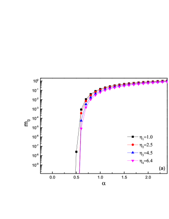
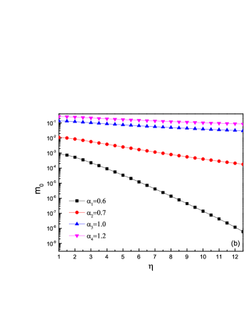
Figure 1: (a) $\alpha$ dependence of $m_{0}$ for different $\eta$; (b) $\eta$ dependence of $m_{0}$ for different $\alpha$. HF approximation is employed.

Figure 2: Phase diagram on $\alpha$-$\eta$ plane under HF approximation.

IV NUMERICAL RESULTS

We utilize the iteration method to solve the DS gap equation numerically. To ensure the reliability of numerical results, we have chosen a series of different initial iteration values. As the gap equation is symmetry under $\eta\rightarrow\frac{1}{\eta}$, we only consider the case of $\eta>1$. The energy scale we adopt here and following , without special mention, is $\bar{v}\Lambda$, here $\Lambda$ is the energy cutoff of momentum integration of mass gap equation.

IV.1 Hartree-Fock approximation

We first consider the HF approximation. The relation between $m_{0}\equiv m(0,0)$ and $\alpha$ obtained at a series of different values of $\eta$ is displayed in Fig. 1(a). In the isotropic case with $\eta=1$, we find that the critical value for dynamical gap generation is roughly $\alpha_{c}\approx 0.5$, which is consistent with Ref. WangJianhui11 . According to Fig. 1(b), $m_{0}$ decreases with increasing of fermion velocity anisotropy. As displayed in Fig. 2, in the parameter space of $\alpha$ and $\eta$, the semimetal phase is enlarged, but the excitonic insulating phase is compressed with the increasing of fermion velocity anisotropy. These results show that fermion velocity anisotropy suppresses dynamical gap generation, which is in contrast with the conclusion under HF approximation given by Ref. Sharma17

IV.2 Instantaneous approximation

The dependence of zero-energy gap $m_{0}$ on $\alpha$ is shown in Fig. 3(a), where several values of $\eta$ are assumed. For $\eta=1$, we find that $\alpha_{c}\approx 2.33$, which is in good agreement with previous results obtained under the instantaneous approximation Khveshchenko01 ; Gorbar02 . The critical value $\alpha_{c}$ under instantaneous approximation is obviously larger than the one under HF approximation, which indicates that the screening from polarization suppresses the dynamical gap generation obviously. As can be observed from Fig. 3(a), $m_{0}$ increases monotonously as $\alpha$ grows. As $\eta$ becomes larger, $m_{0}$ reduces and $\alpha_{c}$ increases.

Then we set the value of $\alpha$ to study the anisotropy dependence of excitonic mass gap. The results are shown in Fig. 3(b). As we can see, for different values of interaction strength, the increase of velocity anisotropy suppresses the formation of dynamical generated gap. Also there is a critical velocity anisotropy $\eta_{c}$, above which the excitonic gap dismisses.

A schematic phase diagram is depicted on the $\alpha$-$\eta$ plane, shown in Fig. 4. There is a critical line between the semimetal phase with vanishing $m_{0}$ and the excitonic insulating phase where $m_{0}\neq 0$. This phase diagram tells us that the dynamical gap can be more easily generated by stronger Coulomb interaction and smaller velocity anisotropy.

The dependence of dynamical gap $m(p_{x},p_{y})$ on the momentum components $|p_{x}|$ and $|p_{y}|$ is displayed in the Fig. 5. Here we choose $\alpha=2.7$. The results obtained at $\eta=1$ and $\eta=2.5$ are presented in Figs. 5 (a) and (b), respectively. In the isotropic case, $m(p_{x},p_{y})$ is symmetric under the transformation $p_{x}\leftrightarrow p_{y}$. However, as shown in Fig. 5(b), the anisotropy of fermion velocities breaks this symmetry.

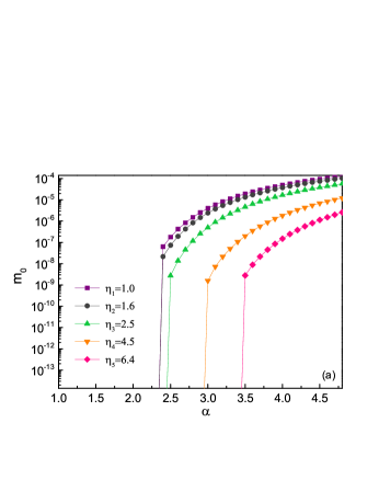
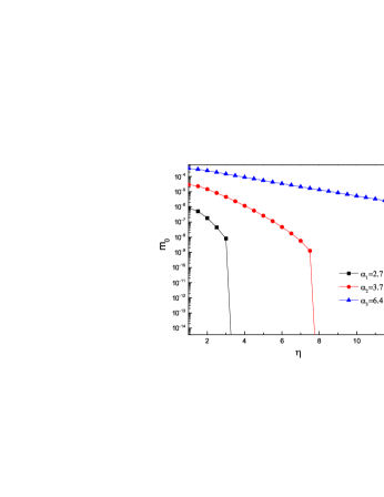
Figure 3: (a) Dependence of $m_{0}$ on $\alpha$ with different $\eta$; (b) Dependence of $m_{0}$ on $\eta$ with different $\alpha$. Instantaneous approximation is taken. $N_{f}=2$ is taken in this figure, and Figs. 4-11.

Figure 4: Phase diagram on $\alpha$-$\eta$ plane under instantaneous approximation.

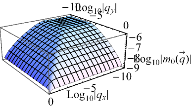
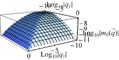
Figure 5: Momentum dependence of mass gap for (a) $\eta=1.0$ and (b) $\eta=2.5$. $\alpha=2.7$ is taken.

IV.3 Gamayun-Gorbar-Guysin (GGG) approximation

For several different values of $\eta$, the curves for the dependence of $m_{0}$ on the Coulomb strength $\alpha$ within GGG approximation are depicted in Fig. 6(a). We can see that there is a critical interaction strength $\alpha_{c}$ above which a finite excitonic gap can be dynamically generated, the magnitude of dynamically generated gap increases with the increasing of interaction strength. It indicates dynamical gap generation appears only if the Coulomb interaction is strong enough. For the isotropic case, we get a critical interaction strength $\alpha_{c}=0.92$, which is in accordance with Ref. Gamayun10 . This critical Coulomb strength is much smaller than the one obtained within instantaneous approximation $\alpha_{c}\approx 2.33$, which reflects that energy dependence of dressed Coulomb interaction promotes the dynamical gap generation. As the velocity anisotropy increases, the magnitude of dynamical gap decreases, and the critical interaction strength increases, which is consistent with the results of instantaneous approximation.

Dependence of $m_{0}$ on the fermion velocity anisotropy $\eta$ with three different values of $\alpha$ is presented in Fig. 6(b). It is easy to find that $m_{0}$ decreases monotonously with growing $\eta$, and is completely suppressed when $\eta$ is larger than a critical value.

Finally, we give the phase diagram in the $\alpha$-$\eta$ plane in Fig. 7. The qualitative characteristic of Fig. 7 is nearly the same as Figs. 2 and 4. All of the three phase diagrams show that increasing the velocity anisotropy leads to a suppression of dynamical gap generation.

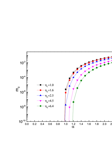
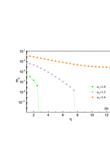
Figure 6: (a) $\alpha$ dependence $m_{0}$ for different $\eta$. (b) $\eta$ dependence of $m_{0}$ for different $\alpha$. GGG approximation is taken.

Figure 7: Phase diagram of $\alpha$ and $\eta$ under GGG approximation.

V Comparison with recent work

In an ideal graphene, the fermions have a universal velocity $v$. Under certain circumstances, there might be an anisotropy and the fermion velocity take different values in different directions. For an isotropic graphene, the velocity anisotropy can be induced by applying uniaxial strain or other manipulations Pereira09 ; Choi10 .

In a recent work, Sharma et al. Sharma17 studied the dynamical gap generation in a uniaxially strained graphene. They have introduced two parameters, namely

$$\alpha_{x}=\frac{e^{2}}{\kappa v_{x}}$$ (28)

and

$$\eta^{\prime}=\frac{1}{\eta}=\frac{v_{y}}{v_{x}}$$ (29)

to characterize the interaction strength and velocity anisotropy. After solving the DS gap equation under the HF and instantaneous approximations, they concluded that at a fixed $\alpha_{x}$, the magnitude of excitonic gap increases monotonously as the parameter $\eta^{\prime}$ decreases from the isotropic case $\eta^{\prime}=1$. They also claimed that the critical value $\alpha_{x}^{c}$ for dynamical gap generation decreases with deceasing $\eta^{\prime}$. Based on these results, Sharma et al. argued that velocity anisotropy is able to promote dynamical gap generation.

We would point out that the analysis made by Sharma et al. is problematic. When the parameter $\alpha_{x}$ is fixed at certain value, the velocity component $v_{x}$ is also fixed. In this case, there are actually two physical effects when lowering $\eta^{\prime}=v_{y}/v_{x}$: first, the velocity component $v_{y}$ decreases; second;, the fermion velocity anisotropy increases. Thus the conclusion that velocity anisotropy supports the formation of excitonic mass actually is a combining effect of lowering the fermion velocity of $v_{y}$ and increasing of fermion velocity anisotropy. In this sense, such conclusion is misleading. According to our calculations, dynamical gap generation is promoted when the fermion velocity decreases, but is suppressed as the anisotropy is enhanced. Therefore, the correct interpretation of the results obtained by Sharma et al. Sharma17 should be: for a fixed $\alpha_{x}$, the promotion of dynamical gap generation caused by decreasing velocity is more important than the suppression caused by the growth of velocity anisotropy.

VI Effects of uniaxial strain on excitonic gap

The fermion velocities of uniaxially strain graphene can be obtained by making first-principle calculations Choi10 . It was found Choi10 that the velocities in the $x$- and $y$-directions vary approximately linearly in strain if the magnitude of strain is smaller than $24\%$. This result is valid when the strain is applied in both $A$ and $Z$ directions Choi10 . For strain $\varepsilon\%$ in $Z$ direction, we can approximate the fermion velocities by the following expressions

$$v_{x} = v_{0}(1+\frac{1}{120}\varepsilon),$$ (30)

$$v_{y} = v_{0}(1-\frac{7}{240}\varepsilon).$$ (31)

Accordingly, the velocity anisotropy parameter $\eta$ and the interaction strength $\alpha$ are re-written as

$$\eta = \frac{1+\frac{1}{120}\varepsilon}{1-\frac{7}{240}\varepsilon},$$ (32)

$$\alpha = \frac{e^{2}}{\kappa v_{0}\sqrt{1-\frac{5\varepsilon}{240}-\frac{7\varepsilon^{2}}{28800}}}$$ (33)

$$= \alpha_{0}\frac{1}{\sqrt{1-\frac{5\varepsilon}{240}-\frac{7\varepsilon^{2}}{28800}}},$$

where $v_{0}$ and $\alpha_{0}$ are the values for graphene without strain. We suppose $\alpha_{0}\approx 2.2$ for suspended graphene. It is easy to verify that both $\alpha$ and $\eta$ increase as the strain grows. Taking advantage of these two relations and the phase diagram in $\alpha-\eta$ plane, we obtain Fig. 8, where the red lines represents the trajectory of interaction strength and velocity anisotropy of suspended graphene under uniaxial strain, and the black line stands for the critical lines on $\alpha-\eta$ plane within instantaneous approximation, respectively. It is clear that, as the uniaxial strain increases, an excitonic gap can be dynamically generated.

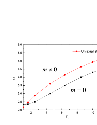
Figure 8: Uniaxial strain effects on interaction strength and velocity anisotropy, combined with phase diagram in the $\alpha-\eta$ plane, obtained under the instantaneous approximation. The red lines represents the trajectory of interaction strength and velocity anisotropy of suspended graphene under uniaxial strain, and the black line stands for the critical lines

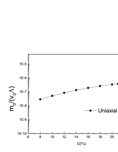
Figure 9: Relation between zero-energy gap $m_{0}$ and strain parameter $\varepsilon$.

The relation between dynamical gap and strain parameter $\varepsilon$ is presented in Fig. 9. The instantaneous approximation is employed in this calculation. In order to compare $m_{0}$ for different interaction strength, we adopt a energy scale of the isotropic case, namely $v_{0}\Lambda$ as the unit of $m_{0}$

The system is gapless when the uniaxial strain is smaller than 7.34$\%$, and a finite dynamical gap is generated as $\varepsilon$ exceeds this critical value. The zero-energy gap $m_{0}$ increases as $\varepsilon$ grows. This implies that applying a uniaxial strain to graphene is in favor of excitonic gap generation, and also that the enhancement effect caused by the decreasing mean velocity dominates over the suppression effect caused by the increasing velocity anisotropy. We notice that the magnitude of dynamical gap $m_{0}$ induced by uniaxial strain is very small, as clearly shown in Fig. 9. Therefore, it would be very difficult to observe such a gap in realistic materials.

VII 2D Dirac semimetal with a tilted cone

It was recently argued Monteverde13 that the organic material $\alpha$-(BEDT-TTF)₂I₃ might be close to a quantum phase transition between semimetallic and excitonic insulating phases due to the smallness of the fermion velocity. In the semimetallic phase of $\alpha$-(BEDT-TTF)₂I₃, the Dirac cone is tilted Tajima09 ; Isobe12 ; Nishine10 ; Sari14 ; Trescher15 ; Proskurin15 ; Hirata17 , which can be considered as a deformation of the perfect Dirac cone realized in an intrinsic graphene. In this section, we examine whether the tilt of Dirac cone favors dynamical gap generation or not.

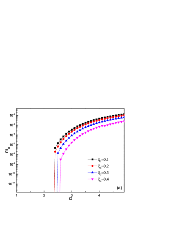
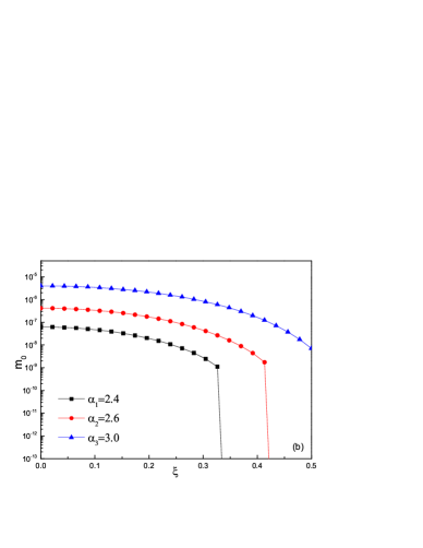
Figure 10: (a) $\alpha$ dependence of $m_{0}$ for different $\xi$. (b) $\xi$ dependence of $m_{0}$ for different $\alpha$.

Figure 11: Phase diagram of $\alpha$ and $\xi$ under instantaneous approximation.

The propagator of fermion excitations around a tiled Dirac cone has the form Isobe12 ; Nishine10 ; Sari14 ; Trescher15 ; Proskurin15 ; Hirata17

$$G(i\omega,\mathbf{k})=\frac{1}{-i\omega\gamma_{0}+v_{0}k_{x}\gamma_{0}+v\mathbf{k}\cdot\mathbf{\gamma}}.$$ (34)

We only consider the case $v_{0}<v$, so that the Fermi surface is still discrete points. For simplicity, we assume that $v_{x}=v_{y}=v$ and focus on the influence of tilt of Dirac cone. The polarization is defined as

$$\Pi(i\Omega,\mathbf{q}) = -N_{f}\int\frac{d\omega}{2\pi}\frac{d^{2}\mathbf{k}}{(2\pi)^{2}}\mathrm{Tr}\big{[}\gamma_{0}G_{0}(i\omega,\mathbf{k})\gamma_{0}$$ (35)

$$\times G_{0}(i\omega+i\Omega,\mathbf{k}+\mathbf{q})\big{]}.$$

According to Ref. Nishine10 , under instantaneous approximation, the polarization is given by

$$\Pi(0,\mathbf{q}) = \frac{N_{f}}{8}\frac{|\mathbf{q}|}{v\sqrt{1-\left(\frac{v_{0}}{v}\right)^{2}\cos^{2}\theta_{\mathbf{q}}}}$$ (36)

$$= \frac{N_{f}}{8}\frac{|\mathbf{q}|}{v\sqrt{1-\left(\frac{v_{0}}{v}\right)^{2}\frac{q_{x}^{2}}{q_{x}^{2}+q_{y}^{2}}}},$$

here $N_{f}=2$. It is then easy to get a dressed Coulomb function

$$V(\mathbf{q}) = \frac{1}{\frac{\kappa|\mathbf{q}|}{2\pi e^{2}}+\Pi(\mathbf{q})}$$ (37)

$$= \frac{1}{\frac{|\mathbf{q}|}{2\pi\alpha v}+\frac{N_{f}}{8}\frac{|\mathbf{q}|}{v\sqrt{1-\left(\frac{v_{0}}{v}\right)^{2}\frac{q_{x}^{2}}{q_{x}^{2}+q_{y}^{2}}}}},$$

where

$$\alpha=\frac{e^{2}}{v\kappa}.$$ (38)

To the leading order, the gap equation is

$$m(p_{x},p_{y}) = \int\frac{d\omega}{2\pi}\int\frac{dk_{x}}{2\pi}\int\frac{dk_{y}}{2\pi}$$ (39)

$$\times\frac{m(k_{y},k_{y})}{\left(\omega+iv_{0}k_{x}\right)^{2}+v^{2}k_{x}^{2}+v^{2}k_{y}^{2}+m^{2}(k_{x},k_{y})}$$

$$\times\frac{1}{\frac{|\mathbf{q}|}{2\pi\alpha v}+\frac{N_{f}}{8}\frac{|\mathbf{q}|}{v\sqrt{1-\left(\frac{v_{0}}{v}\right)^{2}\frac{q_{x}^{2}}{q_{x}^{2}+q_{y}^{2}}}}},$$

where

$$q_{x}=p_{x}-k_{x},\qquad q_{y}=p_{y}-k_{y}.$$ (40)

Performing the integration of $\omega$ by using the contour integral and residue theorem, we obtain

$$m(p_{x},p_{y}) = \frac{1}{2}\int\frac{dk_{x}}{2\pi}\int\frac{dk_{y}}{2\pi}$$ (41)

$$\times\frac{m(k_{y},k_{y})}{\sqrt{v^{2}k_{x}^{2}+v^{2}k_{y}^{2}+m^{2}(k_{x},k_{y})}}$$

$$\times\frac{1}{\frac{|\mathbf{q}|}{2\pi\alpha v}+\frac{N_{f}}{8}\frac{|\mathbf{q}|}{v\sqrt{1-\xi^{2}\frac{q_{x}^{2}}{q_{x}^{2}+q_{y}^{2}}}}},$$

with

$$\xi=\frac{v_{0}}{v}.$$ (42)

Here, we use $\xi$ to measure to what extend the Dirac cone is tilted. $\xi=0$ represents the perfect Dirac cone of graphene, and the increase of $\xi$ stands for the increase of tilted degree of Dirac cone.

The numerical solutions of Eq. (41) are depicted in Fig. 10, which clearly informs us that $m_{0}$ decreases with growing $\xi$. Therefore, the tilt of Dirac cone reduces the possibility of dynamical gap generation. The phase diagram in $\alpha$-$\xi$ plane is presented in Fig. 11.

VIII Summary and discussion

In this paper, we have studied dynamical excitonic gap generation in 2D Dirac semimetal with deformed Dirac cone caused by anisotropy and tilt of Dirac cone. Firstly, we studied dynamical gap generation with anisotropy, which is likely caused by uniaxial strain or periodic potentials. After solving the DS gap equation under three different approximations, we find that the decrease of fermion velocities supports dynamical gap generation, but the velocity anisotropy tends to suppress dynamical gap generation. Subsequently, we have considered the organic material $\alpha$-(BEDT-TTF)₂I₃, which is also a 2D Dirac semimetal, and found that dynamical gap generation is suppressed by the tilt of the Dirac cone. This shows that the shape and geometry of Dirac cone is closely related to the formation of excitonic mass gap generation, which might help to explore concrete materials that can potentially exhibit excitonic insulating transition.

In an uniaxially strained graphene, the fermion dispersion becomes anisotropic. However, it is necessary to emphasize that uniaxial strain leads to not only velocity anisotropy, but also an enhancement of effective Coulomb interaction strength due to the decrease of the mean value of fermion velocity. Dynamical gap generation is suppressed by the former effect, but promoted by the latter one. Therefore, the ultimate influence of uniaxial strain on dynamical gap generation can only be determined by considering these two competitive effects simultaneously. The fate of dynamical gap generation depends on the actual values of $\alpha$ and $\eta$. By adopting the uniaxial strain dependence of fermion velocities in Ref. Choi10 , we show that the overall effects of uniaxial strain can induce an excitonic gap in suspended graphene once the strength of uniaxial strain is over a certain value (namely $7.34\%$). This is in accordance with the results of Sharma et al. Sharma17 . While they have a misinterpretation of the results. It is the decreasing the fermion velocity dominates over the suppression effect caused by the growing velocity anisotropy, and thus induces an excitonic gap, not the velocity anisotropy contributes to the formation of excitonic gap generation.

Our analysis suggest that, a more efficient way to realize excitonic insulating transition is to merely increase the interaction strength by reducing the fermion velocity, without introducing any anisotropy. For instance, one could apply a uniform and isotropic strain on graphene, as suggested in Ref. Tang15 .

- (1) O. Vafek and A. Vishwanath, Annu. Rev. Condens. Matter Phys. 5, 83 (2014).
- (2) T. O. Wehling, A. M. Black-Schaffer, and A. V. Balatsky, Adv. Phys. 63, 1 (2014).
- (3) H. Weng, X. Dai, and Z. Fang, J. Phys.:Condens. Matter 28, 303001 (2016).
- (4) B. Yan and C. Felser, Annu. Rev. Condens. Matter Phys. 8, 337 (2017).
- (5) M. Z. Hasan, S.-Y. Xu, I. Belopolski, and S.-M. Huang, Annu. Rev. Condens. Matter Phys. 8, 289 (2017).
- (6) A. H. Castro Neto, F. Guinea, N. M. R. Peres, K. S. Novoselov, and A. K. Geim, Rev. Mod. Phys. 81, 109 (2009).
- (7) V. N. Kotov, B. Uchoa, V. M. Pereira, F. Guinea, and A. H. Castro Neto, Rev. Mod. Phys. 84, 1067 (2012).
- (8) M. Z. Hasan and C. L. Kane, Rev. Mod. Phys. 82, 3045 (2010).
- (9) X.-L. Qi and S.-C. Zhang, Rev. Mod. Phys. 83, 1057 (2011).
- (10) R. Shankar, Rev. Mod. Phys. 66, 129 (1994).
- (11) J. González, F. Guinea, and M. A. H. Vozmediano, Nucl. Phys. B 424, 595 (1994).
- (12) J. González, F. Guinea, and M. A. H. Vozmediano, Phys. Rev. B 59, 2474(R) (1999).
- (13) D. T. Son, Phys. Rev. B 75, 235423 (2007).
- (14) J. Hofmann, E. Barnes, and S. Das Sarma, Phys. Rev. Lett. 113, 105502 (2014).
- (15) C. Bauer, A. Rückriegel, A. Sharma, and P. Kopietz, Phys. Rev. B 92, 121409(R) (2015).
- (16) A. Sharma and P. Kopietz, Phys. Rev. B 93, 235425 (2016).
- (17) D. C. Elias, R. V. Gorbachev, A. S. Mayorov, S. V. Morozov, A. A. Zhukov, P. Blake, L. A. Ponomarenko, I. V. Grigorieva, K. S. Novoselov, F. Guinea, and A. K. Geim, Nat. Phys. 7, 701 (2011).
- (18) D. A. Siegel, C.-H. Park, C. Hwang, J. Deslippe, A. V. Fedorov, S. G. Louie, and A. Lanzara, Proc. Natl. Acad. Sci. U.S.A. 108, 11365 (2011).
- (19) G. L. Yu, R. Jalil, B. Belle, A. S. Mayorov, P. Blake, F. Schedin, S. V. Morozov, L. A. Ponomarenko, F. Chiappini, S. Wiedmann, U. Zeitler, M. I. Katsnelson, A. K. Geim, K. S. Novoselov, and D. C. Elias, Proc. Natl. Acad. Sci. U.S.A. 110, 3282 (2013).
- (20) D. V. Khveshchenko, Phys. Rev. Lett. 87, 246802 (2001).
- (21) A. H. Castro Neto, Physics 2, 30 (2009).
- (22) E. V. Gorbar, V. P. Gusynin, V. A. Miransky, and I. A. Shovkovy, Phys. Rev. B 66, 045108 (2002).
- (23) D. V. Khveshchenko and H. Leal, Nucl. Phys. B 687, 323 (2004).
- (24) G.-Z. Liu, W. Li, and G. Cheng, Phys. Rev. B 79, 205429 (2009).
- (25) D. V. Khveshchenko, J. Phys.:Condens. Matter 21, 075303 (2009).
- (26) O. V. Gamayun, E. V. Gorbar, and V. P. Gusynin, Phys. Rev. B 81, 075429 (2010).
- (27) J. Sabio, F. Sols, and F. Guinea, Phys. Rev. B 82, 121413(R) (2010).
- (28) C.-X. Zhang, G.-Z. Liu, and M.-Q. Huang, Phys. Rev. B 83, 115438 (2011).
- (29) G.-Z. Liu and J.-R. Wang, New J. Phys. 13, 033022 (2011).
- (30) J.-R. Wang and G.-Z. Liu, J. Phys. Condens. Matter 23, 155602 (2011).
- (31) J.-R. Wang and G.-Z. Liu, J. Phys. Condens. Matter 23, 345601 (2011).
- (32) J.-R. Wang and G.-Z. Liu, New J. Phys. 14, 043036 (2012).
- (33) C. Popovici, C. S. Fischer, and L. von Smekal, Phys. Rev. B 88, 205429 (2013).
- (34) J.-R. Wang and G.-Z. Liu, Phys. Rev. B 89, 195404 (2014).
- (35) J. González, Phys. Rev. B 92, 125115 (2015).
- (36) M. E. Carrington, C. S. Fischer, L. von Smekal, and M. H. Thoma, Phys. Rev. B 94, 125102 (2016).
- (37) O. V. Gamayun, E. V. Gorbar, and V. P. Gusynin, Phys. Rev. B 80, 165429 (2009).
- (38) J. Wang, H. A. Fertig, G. Murthy, and L. Brey, Phys. Rev. B 83, 035404 (2011).
- (39) A. Katanin, Phys. Rev. B 93, 035132 (2016).
- (40) O. Vafek and M. J. Case, Phys. Rev. B 77, 033410 (2008).
- (41) J. González, Phys. Rev. B 82, 155404 (2010).
- (42) J. González, Phys. Rev. B 85, 085420 (2012).
- (43) J. E. Drut and T. A. Lähde, Phys. Rev. Lett. 102, 026802 (2009).
- (44) J. E. Drut and T. A. Lähde, Phys. Rev. B 79, 165425 (2009).
- (45) J. E. Drut and T. A. Lähde, Phys. Rev. B 79, 241405(R) (2009).
- (46) W. Armour, S. Hands, and C. Strouthos, Phys. Rev. B 81, 125105 (2010).
- (47) W. Armour, S. Hands, and C. Strouthos, Phys. Rev. B 84, 075123 (2011).
- (48) P. V. Buividovich and M. I. Polikarpov, Phys. Rev. B 86, 245117 (2012).
- (49) M. V. Ulybyshev, P. V. Buividovich, M. I. Katsnelson, and M. I. Polikarpov, Phys. Rev. Lett. 111, 056801 (2013).
- (50) D. Smith and L. von Smekal, Phys. Rev. B 89, 195429 (2014).
- (51) F. de Juan and H. A. Fertig, Solid State Commun. 152, 1460 (2012).
- (52) A. V. Kotikov and S. Teber, Phys. Rev. D 94, 114010 (2016).
- (53) Y. Nambu and G. Jona-Lasinio, Phys. Rev. 122, 345 (1961).
- (54) V. A. Miransky, Dynamical Symmetry Breaking in Quantum Field Theories, (World Scientific, 1994).
- (55) A. S. Mayorov, D. C. Elias, I. S. Mukhin, S. V. Morozov, L. A. Ponomarenko, K. S. Novoselov, A. K. Geim, and R. V. Gorbachev, Nano. Lett. 12, 4629 (2012).
- (56) M. Monteverde, M. O. Goerbig, P. Auban-Senzier, F. Navarin, H. Henck, C. R. Pasquier, C. Mézière, and P. Batail, Phys. Rev. B 87, 245110 (2013).
- (57) C. Triola, J.-X. Zhu, A. Migliori, and A. V. Balatsky, Phys. Rev. B 92, 045401 (2015).
- (58) H.-K. Tang, E. Laksono, J. N. B. Rodrigues, P. Sengupta, F. F. Assaad, and S. Adam, Phys. Rev. Lett. 115, 186602 (2015).
- (59) V. M. Pereira, A. H. Castro Neto, and N. M. R. Peres, Phys. Rev. B 80, 045401 (2009).
- (60) S.-M. Choi, S.-H. Jhi, and Y.-W. Son, Phys. Rev. B 81, 081407(R) (2010).
- (61) A. Sharma, V. N. Kotov, and A. H. Castro Neto, Phys. Rev. B 95, 235124 (2017).
- (62) C.-H. Park, L. Yang, Y.-W. Son, M. L. Cohen, S. G. Louie, Nat. Phys. 4, 213 (2008).
- (63) C.-H. Park, L. Yang, Y.-W. Son, M. L. Cohen, S. G. Louie, Phys. Rev. Lett. 101, 126804 (2008).
- (64) S. Rusponi, M. Papagno, P. Moras, S. Vlaic, M. Etzkorn, P. M. Sheverdyaeva, D. Pacilé, H. Brune, and C. Carbone, Phys. Rev. Lett. 105, 246803 (2010).
- (65) W. Zhang, R. Yu, W. Feng, Y. Yao, H. Weng, X. Dai, and Z. Fang, Phys. Rev. Lett. 106, 156808 (2011).
- (66) F. Virot, R. Hayn, M. Richter, J. van den Brink, Phys. Rev. Lett. 106, 236806 (2011).
- (67) N. Tajima and K. Kajita, Sce. Technol. Adv. Mater. 10, 024308 (2009).
- (68) H. Isobe and N. Nagaosa, J. Phys. Sco. Jpn. 81, 113704 (2012).
- (69) T. Nishine, A. Kobayashi, and Y. Suzumura, J Phys. Sco. Jpn. 79, 114715 (2010).
- (70) J. Sári, C. Toke, and M. O. Goerbig, Phys. Rev. B 90, 155446 (2014).
- (71) M. Trescher, B. Sbierski, P. W. Brouwer, and E. J. Bergholtz, Phys. Rev. B 91, 115135 (2015).
- (72) I. Proskurin, M. Ogata, and Y. Suzumura, Phys. Rev. B 91, 195413 (2015).
- (73) M. Hirata, K. Ishikawa, G. Matsuno, A. Kobayashi, K. Miyagawa, M. Tamura, C. Berthier, and K. Kanoda, arXiv:1702.00097.