Inverse Reinforcement Learning in Large State Spaces via Function Approximation

Abstract

This paper introduces a new method for inverse reinforcement learning in large-scale and high-dimensional state spaces. To avoid solving the computationally expensive reinforcement learning problems in reward learning, we propose a function approximation method to ensure that the Bellman Optimality Equation always holds, and then estimate a function to maximize the likelihood of the observed motion. The time complexity of the proposed method is linearly proportional to the cardinality of the action set, thus it can handle large state spaces efficiently. We test the proposed method in a simulated environment, and show that it is more accurate than existing methods and significantly better in scalability. We also show that the proposed method can extend many existing methods to high-dimensional state spaces. We then apply the method to evaluating the effect of rehabilitative stimulations on patients with spinal cord injuries based on the observed patient motions.

I Introduction

Approximately 350,000 Americans suffer from serious spinal cord injuries (SCI), resulting in loss of some voluntary motion control. Recently, epidural and transcutaneous spinal stimulation have proven to be promising methods for regaining motor function. To find the optimal stimulation signal, it is necessary to quantitatively measure the effects of different stimulations on a patient. Since motor function is our concern, we mainly study the effects of stimulations on patient motion, represented by a sequence of poses captured by motion sensors. One typical experiment setting is shown in Figure 1, where a patient moves to follow a physician’s instructions, and a sensor records the patient’s center-of-pressure (COP) continuously. This study will assist our design of stimulating signals, as well as advancing the understanding of patient motion with spinal cord injuries.

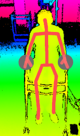
(a) A patient sitting on a sensing device

(b) Instructions on movement directions

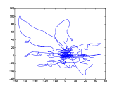
(c) The patient’s COP trajectories during the movement

Figure 1: Rehabilitative game and observed trajectories: in Figure 1a, the patient sits on a sensing device, and then moves to follow the instructed directions in Figure 1b. Figure 1c shows the patient’s center-of-pressure (COP) during the movements.

We assume the stimulating signals will alter the patient’s initial preferences over poses, determined by body weight distribution, spinal cord injuries, gravity, etc., and an accurate estimation of the preference changes will reveal the effect of spinal stimulations on spinal cord injuries, as other factors are assumed to be invariant to the stimulations. To estimate the patient’s preferences over different poses, the most straightforward approach is counting the pose visiting frequencies from the motion, assuming that the preferred poses are more likely to be visited. However, the patient may visit an undesired pose to follow the instructions or to change into a subsequent preferred poses, making preference estimation inaccurate without regarding the context.

In this work, we formulate the patient’s motion as a Markov Decision Process, where each state represents a pose, and its reward value encodes all the immediate factors motivating the patient to visit this state, including the pose preferences and the physician’s instructions. With this formulation, we adopt inverse reinforcement learning (IRL) algorithms to estimate the reward value of each state from the observed motion of the patient.

Existing solutions of the IRL problem mainly work on small-scale problems, by collecting a set of observations for reward estimation and using the estimated reward afterwards. For example, the methods in [1, 2, 3] estimate the agent’s policy from a set of observations, and estimate a reward function that leads to the policy. The method in [4] collects a set of trajectories of the agent, and estimates a reward function that maximizes the likelihood of the trajectories. However, the state space of human motion is huge for non-trivial analysis, and these methods cannot handle it well due to the reinforcement learning problem in each iteration of reward estimation. Several methods [5, 6] solve the problem by approximating the reinforcement learning step, at the expense of a theoretically sub-optimal solution.

The problem can be simplified under the condition that the transition model and the action set remain unchanged for the subject, thus each reward function leads to a unique optimal value function. Based on this assumption, we propose a function approximation method that learns the reward function and the optimal value function, but without the computationally expensive reinforcement learning steps, thus it can be scaled to a large state space. We find that this framework can also extend many existing methods to high-dimensional state spaces.

The paper is organized as follows. We review existing work on inverse reinforcement learning in Section II, and formulate the function approximation inverse reinforcement learning method in large state spaces in III. A simulated experiment and a clinical experiment are shown in Section IV, with conclusions in Section V.

II Related Works

The idea of inverse optimal control is proposed by Kalman [7], white the inverse reinforcement learning problem is firstly formulated in [1], where the agent observes the states resulting from an assumingly optimal policy, and tries to learn a reward function that makes the policy better than all alternatives. Since the goal can be achieved by multiple reward functions, this paper tries to find one that maximizes the difference between the observed policy and the second best policy. This idea is extended by [8], in the name of max-margin learning for inverse optimal control. Another extension is proposed in [2], where the purpose is not to recover the real reward function, but to find a reward function that leads to a policy equivalent to the observed one, measured by the amount of rewards collected by following that policy.

Since a motion policy may be difficult to estimate from observations, a behavior-based method is proposed in [4], which models the distribution of behaviors as a maximum-entropy model on the amount of reward collected from each behavior. This model has many applications and extensions. For example, [9] considers a sequence of changing reward functions instead of a single reward function. [10] and [5] consider complex reward functions, instead of linear one, and use Gaussian process and neural networks, respectively, to model the reward function. [11] considers complex environments, instead of a well-observed Markov Decision Process, and combines partially observed Markov Decision Process with reward learning. [12] models the behaviors based on the local optimality of a behavior, instead of the summation of rewards. [13] uses a multi-layer neural network to represent nonlinear reward functions.

Another method is proposed in [14], which models the probability of a behavior as the product of each state-action’s probability, and learns the reward function via maximum a posteriori estimation. However, due to the complex relation between the reward function and the behavior distribution, the author uses computationally expensive Monte-Carlo methods to sample the distribution. This work is extended by [3], which uses sub-gradient methods to simplify the problem. Another extensions is shown in [15], which tries to find a reward function that matches the observed behavior. For motions involving multiple tasks and varying reward functions, methods are developed in [16] and [17], which try to learn multiple reward functions.

Most of these methods need to solve a reinforcement learning problem in each step of reward learning, thus practical large-scale application is computationally infeasible. Several methods are applicable to large-scale applications. The method in [1] uses a linear approximation of the value function, but it requires a set of manually defined basis functions. The methods in [5, 6] update the reward function parameter by minimizing the relative entropy between the observed trajectories and a set of sampled trajectories based on the reward function, but they require a set of manually segmented trajectories of human motion, where the choice of trajectory length will affect the result. Besides, these methods solve large-scale problems by approximating the Bellman Optimality Equation, thus the learned reward function and Q function are only approximately optimal. We propose an approximation method that guarantees the optimality of the learned functions as well as the scalability to large state space problems.

III Function Approximation Inverse Reinforcement Learning

III-A Markov Decision Process

A Markov Decision Process is described with the following variables:

• $S=\{s\}$, a set of states

• $A=\{a\}$, a set of actions

• $P_{ss^{\prime}}^{a}$, a state transition function that defines the probability that state $s$ becomes $s^{\prime}$ after action $a$.

• $R=\{r(s)\}$, a reward function that defines the immediate reward of state $s$.

• $\gamma$, a discount factor that ensures the convergence of the MDP over an infinite horizon.

A motion can be represented as a sequence of state-action pairs:

$$\zeta=\{(s_{i},a_{i})|i=0,\cdots,N_{\zeta}\},$$

where $N_{\zeta}$ denotes the length of the motion, varying in different observations. Given the observed sequence, inverse reinforcement learning algorithms try to recover a reward function that explains the motion.

One key problem is how to model the action in each state, or the policy, $\pi(s)\in A$, a mapping from states to actions. This problem can be handled by reinforcement learning algorithms, by introducing the value function $V(s)$ and the Q-function $Q(s,a)$, described by the Bellman Equation [18]:

$$V^{\pi}(s)=\sum_{s^{\prime}|s,\pi(s)}P_{ss^{\prime}}^{\pi(s)}[r(s^{\prime})+\gamma*V^{\pi}(s^{\prime})],$$ (1)

$$Q^{\pi}(s,a)=\sum_{s^{\prime}|s,a}P_{ss^{\prime}}^{a}[r(s^{\prime})+\gamma*V^{\pi}(s^{\prime})],$$ (2)

where $V^{\pi}$ and $Q^{\pi}$ define the value function and the Q-function under a policy $\pi$.

For an optimal policy $\pi^{*}$, the value function and the Q-function should be maximized on every state. This is described by the Bellman Optimality Equation [18]:

$$V^{*}(s)=\max_{a\in A}\sum_{s^{\prime}|s,a}P_{ss^{\prime}}^{a}[r(s^{\prime})+\gamma*V^{*}(s^{\prime})],$$ (3)

$$Q^{*}(s,a)=\sum_{s^{\prime}|s,a}P_{ss^{\prime}}^{a}[r(s^{\prime})+\gamma*\max_{a^{\prime}\in A}Q^{*}(s^{\prime},a^{\prime})].$$ (4)

In typical inverse reinforcement learning algorithms, the Bellman Optimality Equation needs to be solved once for each parameter updating of the reward function, thus it is computationally infeasible when the state space is large. While several existing approaches solve the problem at the expense of the optimality, we propose an approximation method to avoid the problem.

III-B Function Approximation Framework

Given the set of actions and the transition probability, a reward function leads to a unique optimal value function. To learn the reward function from the observed motion, instead of directly learning the reward function, we use a parameterized function, named as VR function, to represent the summation of the reward function and the discounted optimal value function:

$$f(s,\theta)=r(s)+\gamma*V^{*}(s),$$ (5)

where $\theta$ denotes the parameter of VR function. The function value of a state is named as VR value.

Substituting Equation (5) into Bellman Optimality Equation, the optimal Q function is given as:

$$Q^{*}(s,a)=\sum_{s^{\prime}|s,a}P_{ss^{\prime}}^{a}f(s^{\prime},\theta),$$ (6)

the optimal value function is given as:

$$V^{*}(s) =\max_{a\in A}Q^{*}(s,a)$$

$$=\max_{a\in A}\sum_{s^{\prime}|s,a}P_{ss^{\prime}}^{a}f(s^{\prime},\theta),$$ (7)

and the reward function can be computed as:

$$r(s) =f(s,\theta)-\gamma*V^{*}(s)$$

$$=f(s,\theta)-\gamma*\max_{a\in A}\sum_{s^{\prime}|s,a}P_{ss^{\prime}}^{a}f(s^{\prime},\theta).$$ (8)

This approximation method is related to value function approximation method in reinforcement learning, but the proposed method can compute the reward function without solving a set of linear equations in stochastic environments.

Note that this formulation can be generalized to other extensions of Bellman Optimality Equation by replacing the $max$ operator with other types of Bellman backup operators. For example, $V^{*}(s)=\log_{a\in A}\exp Q^{*}(s,a)$ is used in the maximum-entropy method[4]; $V^{*}(s)=\frac{1}{k}\log_{a\in A}\exp k*Q^{*}(s,a)$ is used in Bellman Gradient Iteration [19].

For any VR function $f$ and any parameter $\theta$, the optimal Q function $Q^{*}(s,a)$, optimal value function $V^{*}(s)$, and reward function $r(s)$ constructed with Equation (6), (7), and (8) always meet the Bellman Optimality Equation. Under this condition, we try to recover a parameterized function $f(s,\theta)$ that best explains the observed motion $\zeta$ based on a predefined motion model.

Combined with different Bellman backup operators, this formulation can extend many existing methods to high-dimensional spaces, like the motion model based on the value function in [20], $p(a|s)=-v(s)-\log\sum_{k}p_{s,k}\exp(-v(k))$, the reward function in [4], $p(a|s)=\exp{Q(s,a)-V(s)}$, and the Q function in [14]. The main limitation is the assumption of a known transition model $P_{ss^{\prime}}^{a}$, but it only requires a partial model on the experienced states rather than a full environment model, and it can be learned independently in an unsupervised way.

To demonstrate the usage of the framework, this work chooses $max$ as the Bellman backup operator and a motion model $p(a|s)$ based on the optimal Q function $Q^{*}(s,a)$ [14]:

$$P(a|s)=\frac{\exp{b*Q^{*}(s,a)}}{\sum_{\tilde{a}\in A}\exp{b*Q^{*}(s,\tilde{a})}},$$ (9)

where $b$ is a parameter controlling the degree of confidence in the agent’s ability to choose actions based on Q values. In the remaining sections, we use $Q(s,a)$ to denote the optimal Q values for simplified notations.

III-C Function Approximation with Neural Network

Assuming the approximation function is a neural network, the parameter $\theta=\{w,b\}$-weights and biases-in Equation (5) can be estimated from the observed sequence of state-action pairs $\zeta$ via maximum-likelihood estimation:

$$\theta=\operatorname*{argmax}_{\theta}\log{P(\zeta|\theta)},$$ (10)

where the log-likelihood of $P(\zeta|\theta)$ is given by:

$$L_{nn}(\theta) =\log{P(\zeta|\theta)}$$

$$=\log{\prod_{(s,a)\in\zeta}P(a|\theta;s)}$$

$$=\log{\prod_{(s,a)\in\zeta}\frac{\exp{b*Q^{*}(s,a)}}{\sum_{\hat{a}\in A}\exp{b*Q^{*}(s,\hat{a})}}}$$

$$=\sum_{(s,a)\in\zeta}(b*Q(s,a)-\log{\sum_{\hat{a}\in A}\exp{b*Q(s,\hat{a}))}},$$ (11)

and the gradient of the log-likelihood is given by:

$$\nabla_{\theta}L_{nn}(\theta) =\sum_{(s,a)\in\zeta}(b*\nabla_{\theta}Q(s,a)$$

$$-b*\sum_{\hat{a}\in A}P((s,\hat{a})|r(\theta))\nabla_{\theta}Q(s,\hat{a})).$$ (12)

With a differentiable approximation function,

$$\nabla_{\theta}Q(s,a)=\sum_{s^{\prime}|s,a}P_{ss^{\prime}}^{a}\nabla_{\theta}f(s^{\prime},\theta),$$

and

$$\nabla_{\theta}L_{nn}(\theta) =\sum_{(s,a)\in\zeta}(b*\sum_{s^{\prime}|s,a}P_{ss^{\prime}}^{a}\nabla_{\theta}f(s^{\prime},\theta)$$

$$-b*\sum_{\hat{a}\in A}P((s,\hat{a})|r(\theta))\sum_{s^{\prime}|s,a}P_{ss^{\prime}}^{a}\nabla_{\theta}f(s^{\prime},\theta)),$$ (13)

where $\nabla_{\theta}f(s^{\prime},\theta)$ denotes the gradient of the neural network output with respect to neural network parameter $\theta=\{w,b\}$.

If the VR function $f(s,\theta)$ is linear, the objective function in Equation (11) is concave, and a global optimum exists. However, a multi-layer neural network works better to handle the non-linearity in approximation and the high-dimensional state space data.

A gradient ascent method can be used to learn the parameter $\theta$:

$$\theta=\theta+\alpha*\nabla_{\theta}L_{nn}(\theta),$$ (14)

where $\alpha$ is the learning rate.

When the method converges, we can compute the optimal Q function, the optimal value function, and the reward function based on Equation (5), (6), (7), and (8). The algorithm under a neural network-based approximation function is shown in Algorithm 1.

This method does not involve solving the MDP problem for each updated parameter $\theta$, and large-scale state spaces can be easily handled by an approximation function based on a deep neural network.

Algorithm 1 Function Approximation IRL with Neural Network

1:  Data: $\zeta,S,A,P,\gamma,b,\alpha$

2:  Result: optimal value $V[S]$, optimal action value $Q[S,A]$, reward value $R[S]$

3:  create variable $\theta=\{W,b\}$ for a neural network

4:  build $f[S,\theta]$ as the output of the neural network

5:  build $Q[S,A]$, $V[S]$, and $R[S]$ based on Equation (5), (6), (7), and (8).

6:  build loglikelihood $L_{nn}[\theta]$ based on $\zeta$ and $Q[S,A]$

7:  compute gradient $\nabla_{\theta}L_{nn}[\theta]$

8:  initialize $\theta$

9:  while not converging do

10:     $\theta=\theta+\alpha*\nabla_{\theta}L_{nn}[\theta]$

11:  end while

12:  evaluate optimal value $V[S]$, optimal action value $Q[S,A]$, reward value $R[S]$

13:  return $R[S]$

III-D Function Approximation with Gaussian Process

Assuming the VR function $f$ is a Gaussian process (GP) parameterized by $\theta$, the posterior distribution is similar to the distribution in [10]:

$$P(\theta,f_{u}|S_{u},\zeta) \propto P(\zeta,f_{u},\theta|S_{u})$$ (15)

$$=\int_{f_{S}}\underbrace{P(\zeta|f_{S})}_{\text{IRL}}\underbrace{P(f_{S}|f_{u},\theta,S_{u})}_{\text{GP posterior}}df_{S}\underbrace{P(f_{u},\theta|S_{u})}_{\text{GP prior}},$$

where $S_{u}$ denotes a set of supporting states for sparse Gaussian approximation [21], $f_{u}$ denotes the VR values of $S_{u}$, $f_{S}$ denotes the VR values of the whole set of states, and $\theta$ denotes the parameter of the Gaussian process.

Without a closed-form integration, we use the mean function of the Gaussian posterior as the VR value:

$$P(\zeta,f_{u},\theta|S_{u})=P(\zeta|\bar{f_{S}})P(f_{u},\theta|S_{u}),$$ (16)

where $\bar{f_{S}}$ denotes the mean function.

Given a kernel function $k(x_{i},x_{j},\theta)$, the log-likelihood function is given as:

$$L_{gp}(\theta,f_{u})$$ (17)

$$=\log P(\zeta|\bar{f_{S}})+\log P(f_{u},\theta|S_{u})$$ (18)

$$=b*\sum_{(s,a)\in\zeta}(\sum_{s^{\prime}|s,a}P_{ss^{\prime}}^{a}\bar{f(s^{\prime})}-\log{\sum_{\hat{a}\in A}\exp{\sum_{s^{\prime}|s,\hat{a}}P_{ss^{\prime}}^{\hat{a}}\bar{f(s^{\prime}))}}}$$ (19)

$$-\frac{f_{u}^{T}K_{S_{u},S_{u}}^{-1}f_{u}}{2}-\frac{\log|K_{S_{u},S_{u}}|}{2}-\frac{n\log 2\pi}{2}$$ (20)

$$+\log P(\theta),$$ (21)

where $K$ denotes the covariance matrix computed with the kernel function, $\bar{f(s)}=K_{s,S_{u}}^{T}K_{S_{u},S_{u}}^{-1}f_{u}$ denotes the VR value with the mean function $\bar{f_{S}}$, expression (19) is the IRL likelihood, expression (20) is the Gaussian prior likelihood, and expression (21) is the kernel parameter prior.

The parameters $\theta,f_{u}$ can be similarly learned with gradient methods. It has similar properties with neural net-based approach, and the full algorithm is shown in Algorithm 2.

Algorithm 2 Function Approximation IRL with Gaussian Process

1:  Data: $\zeta,S,A,P,\gamma,b,\alpha$

2:  Result: optimal value $V[S]$, optimal action value $Q[S,A]$, reward value $R[S]$

3:  create variable $\theta$ for a kernel function and $f_{u}$ for supporting points

4:  compute $\bar{f(s,\theta,f_{u})}=K_{s,S_{u}}^{T}K_{S_{u},S_{u}}^{-1}f_{u}$

5:  build $Q[S,A]$, $V[S]$, and $R[S]$ based on Equation (5), (6), (7), and (8).

6:  build loglikelihood $L_{gp}[\theta,f_{u}]$ based on Equation (17).

7:  compute gradient $\nabla_{\theta,f_{u}}L_{gp}[\theta,f_{u}]$

8:  initialize $\theta,f_{u}$

9:  while not converging do

10:     $[\theta,f_{u}]=[\theta,f_{u}]+\alpha*\nabla_{\theta,f_{u}}L_{gp}[\theta,f_{u}]$

11:  end while

12:  evaluate optimal value $V[S]$, optimal action value $Q[S,A]$, reward value $R[S]$

13:  return $R[S]$

IV Experiments

We use a simulated environment to compare the proposed methods with existing methods and demonstrate the accuracy and scalability of the proposed solution, then we show how the function approximation framework can extend existing methods to large state spaces. In the end, we apply the proposed method to a clinical application.

IV-A Simulated Environment

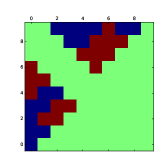
Figure 2: An example of a reward table for one objectworld mdp on a $10\times 10$ grid: it depends on randomly placed objects.

The simulated environment is an objectworld mdp [10]. It is a $N*N$ grid, but with a set of objects randomly placed on the grid. Each object has an inner color and an outer color, selected from a set of possible colors, $C$. The reward of a state is positive if it is within 3 cells of outer color $C1$ and 2 cells of outer color $C2$, negative if it is within 3 cells of outer color $C1$, and zero otherwise. Other colors are irrelevant to the ground truth reward. One example of the reward values is shown in Figure 2. In this work, we place two random objects on a $5*5$ grid, and the feature of a state describes its discrete distance to each inter color and outer color in $C$.

We evaluate the proposed method in three aspects. First, we compare its accuracy in reward learning with other methods. We generate different sets of trajectory samples, and implement the maximum-entropy method in [4], deep inverse reinforcement learning method in [13], and Bellman Gradient Iteration approaches [19]. The VR function based on a neural network has five-layers, where the number of nodes in the first four layers equals to the feature dimensions, and the last layer outputs a single value as the summation of the reward and the optimal value. The VR function based on a Gaussian process uses an automatic relevance detection (ARD) kernel [22] and an uninformed prior, and the supporting points are randomly picked. The accuracy is defined as the correlation coefficient between the ground truth reward value and the learned reward value.

The result is shown in Figure 3. The accuracy is not monotonously increasing as the number of sample grows. The reason is that a function approximator based on a large neural network will overfit the observed trajectory, which may not reflect the true reward function perfectly. During reward learning, we observe that as the loglikelihood increases, the accuracy of the updated reward function reaches the maximum after a certain number of iterations, and then decreases to a stable value. A possible solution to this problem is early-stopping during reward learning. For a function approximator with Gaussian process, the supporting set is important, although an universal solution is unavailable.

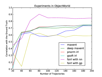
Figure 3: Accuracy comparison with different numbers of observations: ”maxent” denotes maximum entropy method; ”deep maxent” denotes the deep inverse reinforcement learning approach, ”pnorm irl” and ”gsoft irl” denote Bellman Gradient Iteration method; ”fairl with nn” denotes the function approximation inverse reinforcement learning with a neural network; ”fairl with gp” denotes the function approximation inverse reinforcement learning with a Gaussian process.

Second, we evaluate the scalability of the proposed method. Since all these methods involve gradient method, we choose different numbers of states, ranging from 25 to 9025, and compute the time for one iteration of gradient ascent under each state size with each method. ”Maxent” and ”BGI” are implemented with a mix of Python and C programming language; ”DeepMaxent” is implemented with Theano, and ”FAIRL” is implemented with Tensorflow. They all have C programming language in the backend and Python in the forend.

TABLE I: The computation time (second) of one iteration of gradient method under different number of states with different methods: ”Maxent” denotes maximum entropy method, ”DeepMaxent” denotes the deep inverse reinforcement learning approach, ”BGI” denotes Bellman Gradient Iteration method, and ”FAIRLNN” and ”FAIRLGP” denote the function approximation inverse reinforcement learning.

States (#)	Maxent	DeepMaxent	BGI	FAIRLNN	FAIRLGP
25	0.017	0.012	0.0313	0.197	0.331
225	1.831	0.178	2.031	0.397	0.721
625	24.151	0.95	20.963	0.724	1.317
1225	133.839	3.158	102.460	0.921	2.163
2025	474.907	8.119	352.007	0.776	2.332
3025	1319.365	20.253	1061.147	0.762	3.723
4225	3030.723	59.279	2630.309	2.468	4.459
5625	6197.718	101.434	5228.343	2.831	6.495
7225	12234.417	229.752	10147.628	2.217	9.316
9025	20941.9	10466.784	16345.874	3.347	12.372

The result is shown in Table I. Even though the computation time may be affected by different implementations, it still shows that the proposed method is significantly better than the alternatives in scalability, and in practice, it can be further improved by paralleling the computation of the reward function, the value function, and the Q function from the function approximator. Besides, the Gaussian process-based method requires more time than the neural net, because of the matrix inverse operations.

Third, we demonstrate how the proposed framework extends existing methods to large-scale state spaces. We increase the objectworld to a $80*80$ grid, with 10 objects in 5 colors, and generate a large sample set with size ranging from 16000 to 128000 at an interval of 16000. Then we show the accuracy and computation time of inverse reinforcement learning with different combinations of Bellman backup operators and motion models. The combinations include LogSumExp as Bellman backup operator with a motion model based on the reward value [4] and three Bellman backup operators ($max$, $pnorm$, $gsoft$) with a motion model based on the Q values. We do not use even larger state spaces because the generation of trajectories from the ground truth reward function requires a computation-intensive and memory-intensive reinforcement learning step in larger state spaces. A three-layer neural network is adopted for function approximation, implemented with Tensorflow on NVIDIA GTX 1080. The training is done with batch sizes 400, learning rate 0.001, and 20 training epochs are ran. The accuracy is shown in Figure 4. The computation time for one training epoch is shown in Figure 5.

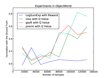
Figure 4: Reward learning accuracy of existing methods in large state spaces: ”LogSumExp”, ”Max”, ”PNorm”, and ”GSoft” are the Bellman backup operators; ”Reward” and ”QValues” are the types of motion models; different combinations of extended methods are plotted. The accuracy is measured as the correlation between the ground truth and the recovered reward.

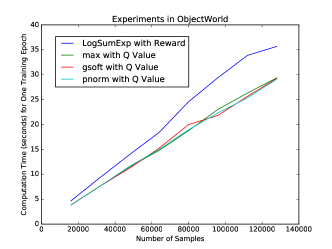
Figure 5: Computation time for one training epoch of existing methods in large state spaces: ”LogSumExp”, ”Max”, ”PNorm”, and ”GSoft” are the Bellman backup operators; ”Reward” and ”QValues” are the types of motion models; different combinations of extended methods are plotted.

The results show that the proposed method achieves accuracy and efficiency simultaneously. In practice, multi-start strategy may be adopted to avoid local optimum.

IV-B Clinical Experiment

In the clinic, a patient with spinal cord injuries sits on a box, with a force sensor, capturing the center-of-pressure (COP) of the patient during movement. Each experiment is composed of two sessions, one without transcutaneous stimulation and one with stimulation. The electrodes configuration and stimulation signal pattern are manually selected by the clinician.

In each session, the physician gives eight (or four) directions for the patient to follow, including left, forward left, forward, forward right, right, right backward, backward, backward left, and the patient moves continuously to follow the instruction. The physician observes the patient’s behaviors and decides the moment to change the instruction.

Six experiments are done, each with two sessions. The COP trajectories in Figure 6 denote the case with four directional instructions; Figure 7, 8, 9, 10, and 11 denote the sessions with eight directional instructions.

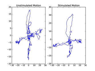
Figure 6: Patient 1 under four directional instructions: ”unstimulated motion” means that the patient moves without transcutaneous stimulations, while ”stimulated motion” represents the motion under stimulations.

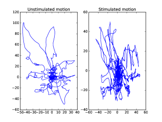
Figure 7: Patient 2 under eight directional instructions: ”unstimulated motion” means that the patient moves without transcutaneous stimulations, while ”stimulated motion” represents the motion under stimulations.

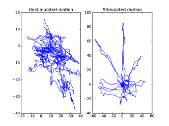
Figure 8: Patient 3 under eight directional instructions: ”unstimulated motion” means that the patient moves without transcutaneous stimulations, while ”stimulated motion” represents the motion under stimulations.

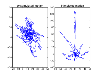
Figure 9: Patient 4 under eight directional instructions: ”unstimulated motion” means that the patient moves without transcutaneous stimulations, while ”stimulated motion” represents the motion under stimulations.

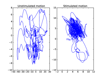
Figure 10: Patient 5 under eight directional instructions: ”unstimulated motion” means that the patient moves without transcutaneous stimulations, while ”stimulated motion” represents the motion under stimulations.

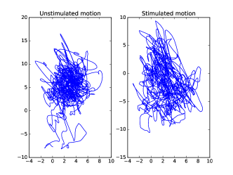
Figure 11: Patient 6 under eight directional instructions: ”unstimulated motion” means that the patient moves without transcutaneous stimulations, while ”stimulated motion” represents the motion under stimulations.

The COP sensory data from each session is discretized on a $100\times 100$ grid, which is fine enough to capture the patient’s small movements. The problem is formulated into a MDP, where each state captures the patient’s discretized location and velocity, and the set of actions changes the velocity into eight possible directions. The velocity is represented with a two-dimensional vector showing eight possible velocity directions. Thus the problem has 80000 states and 8 actions, and the transition model assumes that each action will lead to one state with probability one.

TABLE II: Evaluation of the learned rewards: ”forward” etc. denote the instructed direction; ”1u” denote the patient id ”1”, with ”u” denoting unstimulated session and ”s” denoting stimulated sessions. The table shows the correlation coefficient between the ideal reward and the recovered reward.

	forward	backward	left	right	top left	top right	bottom left	bottom right	origin
1u	-0.352172	-0.981877	-0.511908	-0.399777					-0.0365778
1s	-0.36437	-0.999993	-0.14757	-0.321745					0.154132
2u	-0.459214	-0.154868	0.134229	0.181629	0.123853	0.677538	-0.398259	0.264739	-0.206476
2s	-0.115516	-0.127179	0.569024	0.164638	0.360013	0.341521	0.0817681	0.134049	-0.00986036
3u	0.533031	0.0364088	0.128325	-0.729293	0.397182	0.155565	-0.48818	-0.293617	-0.176923
3s	-0.340902	-0.091139	0.344993	0.0557266	0.162783	0.740827	-0.0897398	-0.00674047	-0.414462
4u	0.099563	-0.0965766	0.145509	-0.912844	0.250434	-0.299531	0.577489	0.134106	-0.151334
4s	-0.258762	-0.019275	-0.263354	0.549305	0.0910128	0.755755	-0.225137	0.289126	-0.216737
5u	0.287442	0.0859648	-0.368503	0.504589	-0.297166	0.401829	0.0583192	-0.23662	-0.0762139
5s	-0.350374	-0.0969275	0.538291	-0.617767	-0.00442265	0.0923481	0.115864	-0.576655	-0.0108339
6u	0.205348	0.302459	0.550447	0.0549231	-0.348898	0.420478	0.378317	0.56191	0.145699
6s	0.105335	-0.155296	0.0193898	-0.283895	-0.0577008	0.220243	-0.31611	-0.296682	-0.0753326

To learn the reward function from the observed trajectories based on the formulated MDP, we use the coordinate and velocity direction of each grid as the feature, and learn the reward function parameter from each set of data. The function approximator is a neural network with three hidden layers and $[100,50,25]$ nodes.

We only test the proposed method with a neural-net function approximator, because it will take prohibitive amount of time to learn the reward function with other methods, and the GP approach relies on the set of supporting points. Assuming it takes only 100 iterations to converge, the proposed method takes about one minute while others run for two to four weeks, and in practice, it may take more iterations to converge.

To compare the reward function with and without stimulations, we adopt the same initial parameter during reward function learning, and run both learning process with 10000 iterations with learning rate 0.00001.

Given the learned reward function, we score the patient’s recovery with the correlation coefficient between the recovered rewards and the ideal rewards under the clinicians’ instructions of the states visited by the patient. The ideal reward for each state is the cosine similarity between the state’s velocity vector and the instructed direction.

The result is shown in Table II. It shows that the patient’s ability to follow the instructions is affected by the stimulations, but whether it is improved or not varies among different directions. The clinical interpretations will be done by physicians.

V Conclusions

This work deals with the problem of inverse reinforcement learning in large state spaces, and solves the problem with a function approximation method that avoids solving reinforcement learning problems during reward learning. The simulated experiment shows that the proposed method is more accurate and scalable than existing methods, and can extends existing methods to high-dimensional spaces. A clinical application of the proposed method is presented.

In future work, we will remove the requirement of a-priori known transition function by combining an environment model learning process into the function approximation framework.

References

- [1] A. Y. Ng and S. Russell, “Algorithms for inverse reinforcement learning,” in in Proc. 17th International Conf. on Machine Learning, 2000.
- [2] P. Abbeel and A. Y. Ng, “Apprenticeship learning via inverse reinforcement learning,” in Proceedings of the twenty-first international conference on Machine learning. ACM, 2004, p. 1.
- [3] G. Neu and C. Szepesvári, “Apprenticeship learning using inverse reinforcement learning and gradient methods,” arXiv preprint arXiv:1206.5264, 2012.
- [4] B. D. Ziebart, A. Maas, J. A. Bagnell, and A. K. Dey, “Maximum entropy inverse reinforcement learning,” in Proc. AAAI, 2008, pp. 1433–1438.
- [5] C. Finn, S. Levine, and P. Abbeel, “Guided cost learning: Deep inverse optimal control via policy optimization,” arXiv preprint arXiv:1603.00448, 2016.
- [6] A. Boularias, J. Kober, and J. R. Peters, “Relative entropy inverse reinforcement learning,” in International Conference on Artificial Intelligence and Statistics, 2011, pp. 182–189.
- [7] R. Kalman and M. M. C. B. D. R. I. for Advanced Studies. Center for Control Theory, When is a Linear Control System Optimal?., ser. RIAS technical report. Martin Marietta Corporation, Research Institute for Advanced Studies, Center for Control Theory, 1963.
- [8] N. D. Ratliff, J. A. Bagnell, and M. A. Zinkevich, “Maximum margin planning,” in Proceedings of the 23rd international conference on Machine learning. ACM, 2006, pp. 729–736.
- [9] Q. P. Nguyen, B. K. H. Low, and P. Jaillet, “Inverse reinforcement learning with locally consistent reward functions,” in Advances in Neural Information Processing Systems, 2015, pp. 1747–1755.
- [10] S. Levine, Z. Popovic, and V. Koltun, “Nonlinear inverse reinforcement learning with gaussian processes,” in Advances in Neural Information Processing Systems 24, J. Shawe-Taylor, R. S. Zemel, P. L. Bartlett, F. Pereira, and K. Q. Weinberger, Eds. Curran Associates, Inc., 2011, pp. 19–27.
- [11] J. Choi and K.-E. Kim, “Inverse reinforcement learning in partially observable environments,” Journal of Machine Learning Research, vol. 12, no. Mar, pp. 691–730, 2011.
- [12] S. Levine and V. Koltun, “Continuous inverse optimal control with locally optimal examples,” arXiv preprint arXiv:1206.4617, 2012.
- [13] M. Wulfmeier, P. Ondruska, and I. Posner, “Deep inverse reinforcement learning,” arXiv preprint arXiv:1507.04888, 2015.
- [14] D. Ramachandran and E. Amir, “Bayesian inverse reinforcement learning,” in Proceedings of the 20th International Joint Conference on Artifical Intelligence, ser. IJCAI’07. San Francisco, CA, USA: Morgan Kaufmann Publishers Inc., 2007, pp. 2586–2591.
- [15] K. Mombaur, A. Truong, and J.-P. Laumond, “From human to humanoid locomotion—an inverse optimal control approach,” Autonomous robots, vol. 28, no. 3, pp. 369–383, 2010.
- [16] C. Dimitrakakis and C. A. Rothkopf, “Bayesian multitask inverse reinforcement learning,” in European Workshop on Reinforcement Learning. Springer, 2011, pp. 273–284.
- [17] J. Choi and K.-E. Kim, “Nonparametric bayesian inverse reinforcement learning for multiple reward functions,” in Advances in Neural Information Processing Systems, 2012, pp. 305–313.
- [18] R. S. Sutton and A. G. Barto, Reinforcement learning: An introduction. MIT press Cambridge, 1998, vol. 1, no. 1.
- [19] K. Li and J. W. Burdick, “Bellman Gradient Iteration for Inverse Reinforcement Learning,” ArXiv e-prints, Jul. 2017.
- [20] E. Todorov, “Linearly-solvable markov decision problems,” in Advances in neural information processing systems, 2007, pp. 1369–1376.
- [21] J. Quiñonero-Candela and C. E. Rasmussen, “A unifying view of sparse approximate gaussian process regression,” Journal of Machine Learning Research, vol. 6, no. Dec, pp. 1939–1959, 2005.
- [22] C. E. Rasmussen and C. K. Williams, Gaussian processes for machine learning. MIT press Cambridge, 2006, vol. 1.