Online Inverse Reinforcement Learning via Bellman Gradient Iteration
Abstract
This paper develops an online inverse reinforcement learning algorithm aimed at efficiently recovering a reward function from ongoing observations of an agent’s actions. To reduce the computation time and storage space in reward estimation, this work assumes that each observed action implies a change of the Q-value distribution, and relates the change to the reward function via the gradient of Q-value with respect to reward function parameter. The gradients are computed with a novel Bellman Gradient Iteration method that allows the reward function to be updated whenever a new observation is available. The method’s convergence to a local optimum is proved. This work tests the proposed method in two simulated environments, and evaluates the algorithm’s performance under a linear reward function and a non-linear reward function. The results show that the proposed algorithm only requires a limited computation time and storage space, but achieves an increasing accuracy as the number of observations grows. We also present a potential application to robot cleaners at home.
I Introduction
Assuming that an agent’s motion in an environment is described with a Markov Decision Process (MDP), the agent may choose an optimal action in a given state based on the reward function of the MDP, as described by reinforcement learning algorithms [1]. However, in many cases, the agent’s actions are observable, while the reward function is hidden and needs to be estimated based on the observed actions, hence the inverse reinforcement learning (IRL) problem. The IRL problem arises in many applications. For example, in robot imitation learning, inverse reinforcement learning algorithms may learn a reward function that explains the operator’s demonstrations, and use the reward function to estimate an optimal control policy for the robot. Another application is human motion analysis, where the reward function that explains a human’s motion may also indicate potential health problems of the subject.
Existing solutions to the IRL problem mainly work in an off-line way, by collecting a set of observations for off-line reward estimation. For example, the methods in [2, 3, 4] estimate the agent’s policy from a set of observations, and estimate a reward function that leads to the policy. The method in [5] collects a set of trajectories of the agent, and estimates a reward function that maximizes the likelihood of the trajectories. This strategy is useful in applications where the learned reward function does not need to be updated frequently.
However, in many applications, such as long-term monitoring of human motion, the observations are available sequentially over an infinite horizon, while the reward function may be needed continuously. In this case, an offline solution needs to store all the past observations and estimate the reward function whenever it is required, which is computationally infeasible. Another scenario is employing a smart service robot that customizes its service based on each user’s preference. Such preferences cannot be modeled a priori, and the preferences may change in a long run, thus an offline solution is infeasible.
To solve the problem, this work formulates an online inverse reinforcement learning algorithm, where the reward function is updated whenever a new observation is available. The proposed method uses an initial reward function to predict the agent’s action distribution, and updates the reward function by increasing the likelihood of the observed action in the predicted distribution. This process is repeated on every new observation, thus the reward function is learned in an online way. This method only stores the latest observation and reward function parameters, and updates the reward parameters once for each new observation. The parameter updating is done by associating the reward parameter and the observation in a differentiable way via Bellman Gradient Iteration. To the best of our knowledge, no previous work solves the inverse reinforcement learning problem in such an online way.
The paper is organized as follows. We review existing methods on inverse reinforcement learning in Section II, and formulate an online inverse reinforcement learning algorithm in Section III. We adopt a Bellman Gradient Iteration method to compute the gradients of Q-values with respect to the reward function in Section IV. Several experiments are shown in Section V, with conclusions in Section VI.
II Related Works
The idea of inverse optimal control is proposed by Kalman [6], while the Inverse Reinforcement Learning problem is first formulated in [2], where the agent observes the states resulting from an assumingly optimal policy, and tries to learn a reward function that makes the policy better than all alternatives. Since the goal can be achieved by multiple reward functions, this paper tries to find one that maximizes the difference between the observed policy and the second best policy. This idea is extended by [7], in the name of max-margin learning for inverse optimal control. Another extension is proposed in [3], where the goal is not necessarily to recover the actual reward function, but to find a reward function that leads to a policy equivalent to the observed one, measured by the total reward collected by following that policy. These solutions cannot solve the IRL problem in an online way, because the policy needs to be estimated from a set of observations.
Since a motion policy may be difficult to estimate from observations, a behavior-based method is proposed in [5], which models the distribution of behaviors as a maximum-entropy model on the amount of reward collected from each behavior. This model has many applications and extensions. For example, Nguyen et al. [8] consider a sequence of changing reward functions instead of a single reward function. Levine et al. [9] and Finn et al. [10] consider complex reward functions, instead of linear ones, and use Gaussian process and neural networks, respectively, to model the reward function. Choi et al. [12] consider partially observed environments, and combines a partially observed Markov Decision Process with reward learning. Levine et al. [13] model the behaviors based on the local optimality of a behavior, instead of the summation of rewards. Wulfmeier et al. [14] use a multi-layer neural network to represent nonlinear reward functions. These solutions update the reward function based on the whole trajectory of an agent, thus it cannot solve the IRL problem in an online way.
Another method is proposed in [15], which models the probability of a behavior as the product of each state-action’s probability, and learns the reward function via maximum a posteriori estimation. However, due to the complex relation between the reward function and the behavior distribution, the author uses computationally expensive Monte-Carlo methods to sample the distribution. This work is extended by [4], which uses sub-gradient methods to reduce the computations. Another extensions is shown in [16], which tries to find a reward function that matches the observed behavior. For motions involving multiple tasks and varying reward functions, methods are developed in [17] and [18], which try to learn multiple reward functions. These solutions also depend on the policy of the agent, thus an online extension is difficult to formulate.
The method proposed in this paper models the distribution of the state-action pairs based on Q-values, and updates the reward for each observed action with gradient methods like [4], but the proposed approach adopts two approximation methods that improve the flexibility of action modeling, and develops a Bellman Gradient Iteration algorithm that computes the gradient of the optimal value function and the optimal Q-function with respect to the reward function accurately and efficiently. Besides, we show how the approximate affects the learned reward function parameters, and give the conditions for the approximation to be more accurate. This work is an extension of our previous work [11].
III Online Inverse Reinforcement Learning
III-A Markov Decision Process
We assume that an agent’s motion in an environment can be described with a Markov Decision Process, defined by the following variables:
-
•
, a set of states
-
•
, a set of actions
-
•
, a state transition function that defines the probability that state becomes after action .
-
•
, a reward function that defines the immediate reward of state .
-
•
, a discount factor that ensures the convergence of the MDP over an infinite horizon.
Given the observed actions of the agent, inverse reinforcement learning algorithms aim to recover the reward function that explains the actions. In long-term applications, the agent’s actions are often observed sequentially, and the reward function needs to be estimated in an online way. This work formulates the following online inverse reinforcement learning algorithm:
-
•
given reward function at moment , observe current state and predict a distribution of actions .
-
•
observe the true action taken by the agent.
-
•
update the reward function to to increase the likelihood of action .
To model the distribution , it is necessary to relate a state-action pair with the reward function . This problem can be handled in reinforcement learning algorithms by introducing the value function and the Q-function , described by the Bellman Equation [1]:
| (1) | |||
| (2) |
where and define the value function and the Q-function under a policy , defined as a mapping from the set of states to the set of actions , which describes the probabilities of actions to take in a state.
For an optimal policy , the value function and the Q-function should be optimized on every state. This is described by the Bellman Optimality Equation [1]:
| (3) | |||
| (4) |
III-B Online Reward Learning
We assume that reward function can be expressed as a function of a finite dimensional parameter vector to parameterize the reward function at time , and the reward function can be a linear or non-linear function. This work models the predicted action distribution with the method in [15], based on the optimal Q-value under parameter :
| (5) |
where is a parameter controlling the degree of confidence in the agent’s ability to choose actions based on Q values. For simplification of notation, in the remaining sections, denotes the optimal Q-value of the state-action pair under reward parameter .
Under this prediction, the likelihood of the agent’s action is given by:
| (6) |
and its log-likelihood is given by:
| (7) |
To increase this log-likelihood, is improved by an amount proportional to the gradient of the log-likelihood for each new observation:
| (8) |
where is the learning rate, and the gradient of the log-likelihood is given by:
| (9) |
To compute the gradient, it is necessary to compute the gradient of the Q-function . The standard way to compute the optimal Q-value is with the Bellman Equation of Optimality in Equation (4).
However, the Q-value in Equation (4) is non-differentiable with respect to or due to the max operator. Its gradient cannot be computed in a conventional way, and the sub-gradient method in [4] cannot compute the gradients everywhere in the parameter space. This work introduces a method called Bellman Gradient Iteration to solve the problem.
IV Bellman Gradient Iteration
To handle the non-differentiable max function in Equation (4), this work adopts two approximation methods. After introducing these approximations, we analyze their approximating qualities.
IV-A Approximation with a P-Norm Function
The first approximation is based on a p-norm:
| (10) |
where controls the level of approximation, and all the values are assumed to be positive. When , the approximation becomes exact. In the remaining sections, this method is called a p-norm approximation.
Under this approximation, the Q-function in Equation (4) can be rewritten as:
| (11) |
From Equation (11), we can construct an approximately optimal value function with p-norm approximation :
| (12) |
Equations (11) and (12) lead to an approximate Bellman Optimality Equation to find the approximately optimal value function and Q-function:
| (13) | |||
| (14) |
Taking the derivative of both sides of Equation (12) and Equation (13), the gradients of and with respect to reward function parameter are:
| (15) | |||
| (16) |
For a p-norm approximation with non-negative Q-values, the gap between the approximate value function and the optimal value function is a function of :
The gap function describes the error of the approximation, and it has two properties.
Proposition 1
Assuming , the tight lower bound of is zero:
Proposition 2
Assuming all Q-values are non-negative, , is a decreasing function with respect to increasing :
The proof is given in Appendix -A.
IV-B Approximation with Generalized Soft-Maximum Function
The second approximation is based on a generalized soft-maximum function:
| (17) |
where controls the level of approximation. When , the approximation becomes exact. The remaining sections refer to this method as g-soft approximation.
Under this approximation, the Q-function in Equation (4) can be rewritten as:
| (18) |
Based on Equation (18), an approximately optimal value function with g-soft approximation takes the form:
| (19) |
Equations (18) and (19) leads to an approximate Bellman Optimality Equation to find the approximately optimal value function and Q-function:
| (20) | |||
| (21) |
Taking derivative of both sides of Equations (19) and (20) yields a Bellman Gradient Equation to compute the gradients of and with respect to the reward function parameter :
| (22) | |||
| (23) |
For a g-soft approximation, the gap between the approximate value function and the optimal value function is:
The gap has the same two properties as the p-norm approximation.
Proposition 3
The tight lower bound of is zero:
Proposition 4
is a decreasing function with respect to increasing :
The proof is given in Appendix -B.
Approximating properties of Bellman Gradient Iteration shows that the gap between the approximated Q-value and the exact Q-value decreases with larger . Thus the value of objective function in Equation (7) under approximation will approach the true one with larger .
Under the approximation, the objective function in Equation (7) converges to within some range of a locally optimal value with the gradient method. Formally:
Proposition 5
Assuming is a local optimum of the objective function under the true Q function and is the locally optimal value, the gradient method from a starting point in basin of a under the approximated gradient will converge to , such that and .
The proof is given in Appendix -C. These proofs show that the approximated gradient converges to a point whose distance to the converged point under the true gradient is infinitesimal with a sufficiently large approximation level .
IV-C Bellman Gradient Iteration
Based on the Bellman Equations (13), (14), (20), and (21), we can iteratively compute the value of each state and the value of each state-action pair under reward parameter , as shown in Algorithm 2. In the algorithm, means a p-norm approximation of the max function for the first method, and a g-soft approximation of the max function for the second method.
After computing the approximately optimal Q-function, with the Bellman Gradient Equation (15), (16), (22), and (23), we can iteratively compute and with respect to the reward function parameter , as shown in Algorithm 3. In the algorithm, corresponds to the gradient of each approximate value function with respect to the function, as shown in Equation (15) and Equation (22).
In these two approximations, the value of parameter depends on an agent’s ability to choose actions based on the Q values. Without application-specific information, we choose as an uninformed parameter. Given a value for parameter , the motion model of the agent is defined on the approximated Q values, where the Q-value of a state-action pair depends on both the optimal path following the state-action pair and other paths. When the approximation level is smaller, the Q-value of a state-action pair relies less on the optimal path, and the motion model in Equation (5) is similar to the model in [5]; When , the Q-value approaches the standard Q-value, and the motion model is similar to the model in [15]. By choosing different values, we can adapt the algorithm to different types of motion models.
With empirically chosen application-dependent parameters and , Algorithm 2 and Algorithm 3 are used compute the gradient of each Q-value, , with respect to the reward function parameter , and then the parameter is learned with the gradient ascent method shown in Equation (7) and Equation (8). A multi-start strategy handles local optimum. This process is shown in Algorithm 1.
V Experiments
We test the proposed method in two benchmark environments to evaluate its accuracy, and then show a potential application to a smart home cleaning robot.
V-A Benchmark Environments
We evaluated the proposed method in two existing benchmark environments.
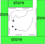
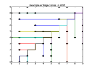
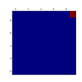
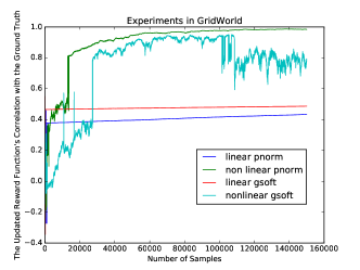
The first example environment is a parking space behind a store, as shown in Figure 1a. At each moment, a mobile robot tries to generate an estimation of the location of the exit based on the observed motions of multiple agents, like cars. Assuming that the true exit is in one corner of the space, we can describe it with the gridworld mdp [2], and solve the problem via online inverse reinforcement learning. In this grid, the true but a-priori unknown rewards for all states equal to zero, except for the upper-right corner state, whose reward is one, corresponding to the true exit, as shown in Figure 2a. Each agent starts from a random state, and chooses in each step one of the following actions: up, down, left, and right. Some trajectories are shown in Figure 1b. Each action has a 30% probability that a random action from the set of actions is actually taken. For inverse reinforcement learning, we compare a linear function and a non-linear function to represent the reward, where the feature of a state is a length- vector indicating the position of the grid represented by the state, e.g., the element of the feature vector for the state equals to one and all other elements are zeros. The non-linear function is given as a neural network with two hidden layers, each with 10 nodes.
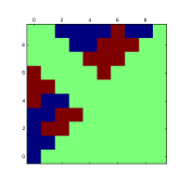
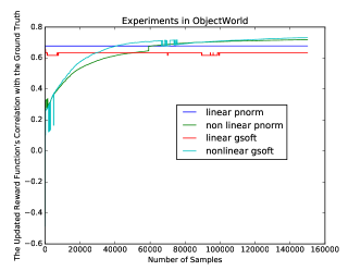
The second environment is an objectworld mdp [9]. It is similar to the gridworld mdp, but with a set of objects randomly placed on the grid. Each object has an inner color and an outer color, selected from a set of possible colors, . The reward of a state is positive if it is within 3 cells of outer color and 2 cells of outer color , negative if it is within 3 cells of outer color , and zero otherwise. Other colors are irrelevant to the ground truth reward. One example is shown in Figure 2b. This work places two random objects on the grid, and compares a linear function and a nonlinear function to represent the reward, where the feature of a state indicates its discrete distance to each inter color and outer color in . The non-linear function is given as a neural network with two hidden layers, each with 10 nodes.
V-B Results
To evaluate the utility of the proposed algorithm, we use correlation coefficients to measure the similarity between the learned reward and the true rewards at each moment.
In each environment, 150,000 state-action pairs are generated based on the true rewards. To simulate a long-term real world observation, we do not assume the environment state to be static if without robot actions; instead, it is randomly changed every three observations, and the agent has to choose a sequence of actions reactively.
We run the proposed algorithm on the data collected from each environment with 30 random initializations simultaneously, and for each new observation, the correlation coefficient between the ground truth and the reward function with the highest likelihood among the 30 candidates is recorded. Besides, we test the algorithm with two approximation methods, pnorm and gsoft, and test each approximation method with a linear reward function and a nonlinear reward function. For the linear reward function, we manually choose the learning rate as 0.00001 in both environments, and for the nonlinear reward function, the learning rate is chosen as 0.001. The approximation parameters are chosen as . The results are plotted in Figure 3 and 4.
The results show that the accuracy of the learned reward increases as the observation time increases. While the accuracy reaches the optimum point faster under a linear reward function, the accuracy is higher under a non-linear reward function.
V-C Smart Home Cleaning Robot
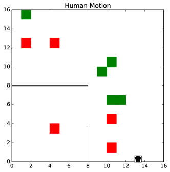
We create a simulated home environment with a person inside and show how the proposed method improves the efficiency of a home cleaning robot.
Many existing robot cleaners move around the home uniformly, to make sure that every area is evenly covered. However, this may be inefficient since some areas require more attention while other areas need less work. To rank different home areas, we assume that more cleaning should be done in areas which are more frequently visited, and such preference is learned by observing the human activity via inverse reinforcement learning. Since the preference varies among different users, the cleaning robot needs to learn it in an online way after being employed.
The room environment is composed of walls and spaces, and there are furnitures that affect the preference of the person, as shown in Figure 5. This environment is discretized into a grid, where the robot can intermittently observe the movement of the person, and update its internal reward function based on each new observation. We simulate 5000 human actions, and the robot uses the g-soft approximation with to learn the reward function. A linear reward function and a nonlinear reward function based on a three layer neural network, with twenty nodes in each layer, are adopted during online inverse reinforcement learning. Ten initial starting parameters are adopted for each reward function, and at each step, the reward leading to the highest likelihood is output. The online learned reward function is visualized in the attached video.
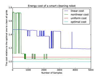
Assuming that the floor’s dirt level is distributed as the true reward function and the robot need to clean all the grids to make the dirt level equal to zero, we evaluate the proposed method based on the consumed energy in cleaning. The energy cost is computed based on how many times the robot needs to sweep the whole area, with different dirt distributions, to make every corner clean. We compare the accumulated energy consumption by following the uniform cleaning approach, the optimal approach with the true reward, the proposed approach with a linear reward function, and the proposed approach with a non-linear reward function. The result in given in Figure 6.
It shows that with a non-linear reward function, the cleaning robot consumes less energy than the typical uniform approach. The amount of saved energy depends negatively on the uniformity of the true reward function.
.
VI Conclusions
This work formulates an online inverse reinforcement learning algorithm to estimate a reward functions based on sequentially observed actions of an agent. For each new observation, a predicted action distribution is computed based on previous reward function, and the reward function is updated to increase the likelihood of the newly observed action. The action distribution is formulated as a function of the optimal Q-value, and the gradient of the optimal Q-value with respect to the reward function is computed via Bellman Gradient Iteration. The algorithm is tested in two simulated environments based on two approximation methods. The result shows that the proposed method gradually approaches the true reward function as the number of samples increases, but only requires limited storage space and computation time. A potential application to home cleaning robots is demonstrated.
In future work, we will explore different variants of stochastic gradient descent for online inverse reinforcement learning, and apply the method to several long-term applications, like human motion analysis.
References
- [1] R. S. Sutton and A. G. Barto, Reinforcement learning: An introduction. MIT press Cambridge, 1998, vol. 1, no. 1.
- [2] A. Y. Ng and S. Russell, “Algorithms for inverse reinforcement learning,” in in Proc. 17th International Conf. on Machine Learning, 2000.
- [3] P. Abbeel and A. Y. Ng, “Apprenticeship learning via inverse reinforcement learning,” in Proceedings of the twenty-first international conference on Machine learning. ACM, 2004, p. 1.
- [4] G. Neu and C. Szepesvári, “Apprenticeship learning using inverse reinforcement learning and gradient methods,” arXiv preprint arXiv:1206.5264, 2012.
- [5] B. D. Ziebart, A. Maas, J. A. Bagnell, and A. K. Dey, “Maximum entropy inverse reinforcement learning,” in Proc. AAAI, 2008, pp. 1433–1438.
- [6] R. Kalman and M. M. C. B. D. R. I. for Advanced Studies. Center for Control Theory, When is a Linear Control System Optimal?., ser. RIAS technical report. Martin Marietta Corporation, Research Institute for Advanced Studies, Center for Control Theory, 1963.
- [7] N. D. Ratliff, J. A. Bagnell, and M. A. Zinkevich, “Maximum margin planning,” in Proceedings of the 23rd international conference on Machine learning. ACM, 2006, pp. 729–736.
- [8] Q. P. Nguyen, B. K. H. Low, and P. Jaillet, “Inverse reinforcement learning with locally consistent reward functions,” in Advances in Neural Information Processing Systems, 2015, pp. 1747–1755.
- [9] S. Levine, Z. Popovic, and V. Koltun, “Nonlinear inverse reinforcement learning with gaussian processes,” in Advances in Neural Information Processing Systems 24, J. Shawe-Taylor, R. S. Zemel, P. L. Bartlett, F. Pereira, and K. Q. Weinberger, Eds. Curran Associates, Inc., 2011, pp. 19–27.
- [10] C. Finn, S. Levine, and P. Abbeel, “Guided cost learning: Deep inverse optimal control via policy optimization,” arXiv preprint arXiv:1603.00448, 2016.
- [11] K. Li and J. W. Burdick, “Bellman Gradient Iteration for Inverse Reinforcement Learning,” ArXiv e-prints, Jul. 2017.
- [12] J. Choi and K.-E. Kim, “Inverse reinforcement learning in partially observable environments,” Journal of Machine Learning Research, vol. 12, no. Mar, pp. 691–730, 2011.
- [13] S. Levine and V. Koltun, “Continuous inverse optimal control with locally optimal examples,” arXiv preprint arXiv:1206.4617, 2012.
- [14] M. Wulfmeier, P. Ondruska, and I. Posner, “Deep inverse reinforcement learning,” arXiv preprint arXiv:1507.04888, 2015.
- [15] D. Ramachandran and E. Amir, “Bayesian inverse reinforcement learning,” in Proceedings of the 20th International Joint Conference on Artifical Intelligence, ser. IJCAI’07. San Francisco, CA, USA: Morgan Kaufmann Publishers Inc., 2007, pp. 2586–2591.
- [16] K. Mombaur, A. Truong, and J.-P. Laumond, “From human to humanoid locomotion—an inverse optimal control approach,” Autonomous robots, vol. 28, no. 3, pp. 369–383, 2010.
- [17] C. Dimitrakakis and C. A. Rothkopf, “Bayesian multitask inverse reinforcement learning,” in European Workshop on Reinforcement Learning. Springer, 2011, pp. 273–284.
- [18] J. Choi and K.-E. Kim, “Nonparametric bayesian inverse reinforcement learning for multiple reward functions,” in Advances in Neural Information Processing Systems, 2012, pp. 305–313.
-A P-Norm Approximation
Assuming , the tight lower bound of is zero:
Proof:
, assuming ,
Since ,
When :
∎
Assuming all Q-values are non-negative, , is a decreasing function with respect to increasing :
Proof:
Since :
∎
-B G-Soft Approximation
The tight lower bound of is zero:
Proof:
: assuming
When ,
∎
is a decreasing function with respect to increasing :
Proof:
Since:
∎
-C Convergence Analysis
Assuming is a local optimum of the objective function under the true Q function and is the locally optimal value, the gradient method from a starting point in basin of a under the approximated gradient will converge to , such that and .
Proof:
First, we show that the gradient method will converge to a point under the approximated gradient. We consider the case when the objective function is defined on one state-action pair, but the result can be easily applied to general cases.
Stochastic gradient methods update the reward parameter once for each observation. For a update step , we expand the updated objective function with first-order Taylor series:
| (24) |
where
| (25) |
| (26) |
denotes the approximate gradient under p-norm approximation or g-soft approximation.
Due to the max-operation in Bellman Optimality Equation, is a piecewise smooth function of , and the gradient is defined on the optimal paths following under current , while is defined on both the optimal path and all the other non-optimal paths following . We describe as a weighted summation of the optimal paths and the non-optimal paths, where the weight is a function of :
| (27) |
where denotes the state action pairs in the non-optimal paths, and
As increases, will depends more on the optimal paths, thus will increase while will decrease. When , and .
This description is reasonable based on Equation (15), (16) (22), and (23), where in each iteration, the approximate gradient of a state-action pair is defined as a weighted summation of the gradients of the resultant state-action pairs, and the weights of the optimal ones approach 1 as increases, thus the final approximated gradient can be described as a weighted summation of the optimal sequences of state-action pairs and other sequences.
Assuming , in the best case, if the two gradients have the same direction, the improvement is ; in the worst case, if they have the opposite directions, the improvement is . Therefore, the improvement of the objective function depends on . If for a sufficiently large , we can make sure that the objective function is converging:
The convergence rate depends on , , and the MDP structure.
Second, we show that .
We construct an approximate objective function by replacing the Q value in Equation (7) with an approximated Q value:
where denotes the approximate gradient under p-norm approximation or g-soft approximation. is a differentiable equation and a local optimum can be reached via gradient method.
Based on proposition 1, 2, 3, and 4, we propose that . Thus the following inequality holds:
| (29) |
Therefore, , we may choose a leading to . This will guarantee for any . Since and represent two close local optimum points, we deduce that .
Wih Taylor expansion,
Thus,
and,
∎